Exponential Consensus of Multiple Agents over Dynamic Network Topology: Controllability, Connectivity, and Compactness
Abstract
This paper investigates the problem of securing exponentially fast consensus (exponential consensus for short) for identical agents with finite-dimensional linear system dynamics over dynamic network topology. Our aim is to find the weakest possible conditions that guarantee exponentially fast consensus using a Lyapunov function consisting of a sum of terms of the same functional form. We first investigate necessary conditions, starting by examining the system (both agent and network) parameters. It is found that controllability of the linear agents is necessary for reaching consensus. Then, to work out necessary conditions incorporating the network topology, we construct a set of Laplacian matrix-valued functions. The precompactness of this set of functions is shown to be a significant generalization of existing assumptions on network topology, including the common assumption that the edge weights are bounded piecewise constant functions or continuous functions. With the aid of such a precompactness assumption and restricting the Lyapunov function to one consisting of a sum of terms of the same functional form, we prove that a joint -connectivity condition on the network topology is necessary for exponential consensus. Finally, we investigate how the above two “necessities” work together to guarantee exponential consensus. To partially address this problem, we define a synchronization index to characterize the interplay between agent parameters and network topology. Based on this notion, it is shown that by designing a proper feedback matrix and under the precompactness assumption, exponential consensus can be reached globally and uniformly if the joint -connectivity and controllability conditions are satisfied, and the synchronization index is not less than one.
Index Terms:
Exponential consensus, controllable linear systems, dynamic network topology, precompactness, necessary and sufficient condition.I Introduction
Consensus is ubiquitous in distributed control, estimation, and computation, see [1] and [2], as representatives of a massive literature. It refers to agreement of a network of individual agents on a quantity of interest, e.g., position, opinion, and estimation [2, 3]. Over the last decades, consensus analysis has attracted significant attentions in systems and control and also in social network analysis [4, 5, 6, 7, 8].
Very recently, it has been found applicable to various interesting scenarios, for example shortest path planning [10], distributed optimization algorithm design [11], and resilient estimation under attack over networks [12]. These potential applications, consequently, motivate further investigation of coordination/cooperation of networked agents. With this inspiration, in this paper we focus on development of the weakest possible conditions to guarantee exponentially fast consensus; the exponential property is generally desirable and offers better performance and more robustness against noise, parameter perturbations, nonlinearity, etc. Such weak conditions also help us gain insight into how the networked high-order111In this paper, “high-order” means that each agent has high-order dynamics. Note that to follow convention, the networked linear agents are described by first-order differential equations and their states have a high dimension. linear agents interact with each other and evolve.
To date, various necessary and/or sufficient connectivity conditions for achieving consensus under dynamic network topology (i.e., the edge weights are functions of time) have been developed for integrator agents [8, 13, 14, 15, 16, 17]. Of particular interest is the joint -connectivity condition (refer to Definition 3 in the next section). It is shown in [15] to be necessary and sufficient for exponential consensus of continuous-time integrator agents with undirected dynamic network topology. Therefore, it is of theoretical interest to analyze whether joint -connectivity is still necessary for exponential consensus of high-order linear agents. This question also motivates the current work.
Achieving consensus for high-order linear systems with self-dynamics over a dynamic network topology has been studied over the past decades. Existing literature usually imposes stringent conditions on system parameters (including system and input matrices) [18, 19, 20, 21, 22, 23, 24] or network topology [25, 5, 26, 27, 46]. A frequent connectivity condition or a well-defined averaged connectivity condition is commonly proposed to accommodate consensus analysis [9, 25, 5, 26]. For instance, piecewise continuous networks are assumed to have uniformly bounded weights [46], i.e., the connectivity of the network topology remains unchanged. Other works usually carry out consensus analysis with a full-rank input matrix [18] or a non-expansive system matrix. Synchronizing heterogeneous systems is taken into consideration in [20, 21, 24], and [22]. By designing full-state coupled dynamic controllers or reference signals, the synchronization problem is transformed into a consensus problem for integrator agents [20, 21, 24, 22]. Recently, consensus of nonexpansive time-varying finite-dimensional linear agents with a full-rank input matrix was investigated in [23]. A common weakness of the above works [18, 19, 20, 21, 22, 23, 24] is that the coupling configurations take full-state coupled forms. This relaxes the assumption on network connectivity and makes the consensus analysis easier.
If the input matrix takes non-full row rank and simultaneously a weak connectivity assumption is imposed, as far as we know, most results reported for consensus of high-order linear systems are based on having an undirected network topology [28, 29, 30, 31]. In [28], marginally stable linear systems with a non-full row rank input matrix are considered. These linear agents communicate over piecewise constant network topology with a positive dwell time (see Section III for the definition of “dwell time”). The authors prove that, with a properly chosen feedback matrix, as long as a uniform connectivity condition (a special case of joint -connectivity) and an observability condition are satisfied, asymptotic consensus can be ensured [28]. Consensus of neutrally stable linear systems over either piecewise constant network topology or continuously time-varying network topology (i.e., edge weights are continuous functions of time) has recently been studied in [31] and [30], separately. A subspace-based method [30] and a uniform complete observability-based approach [31] are, respectively, developed. With these methods, necessary and sufficient conditions for consensus have been successfully derived [31, 30]. In [29], it is assumed that the network topology is piecewise constant with a positive dwell time. The constraint on the system matrix is relaxed such that the linear agents only need to be controllable [29]. The authors show that consensus can be reached asymptotically with a suitably designed feedback matrix if the Lyapunov exponent is less than the synchronizability exponent, which is defined to describe a quantitative characteristic of the network topology [29].
To conclude, although impressive advances have been made [28, 29, 31, 30] for consensus analysis of finite-dimensional linear systems over an undirected dynamic network topology, there are still several issues left for further consideration. First, consensus conditions imposed on the network topology or system parameters are still stringent, e.g., the existence of a positive dwell time [29]. Second, necessary conditions for convergence to consensus have rarely been considered.
With the above motivation, we revisit the consensus problem of linear systems under the framework of undirected networks. We restrict attention to undirected graphs because (a) how to handle the directed case is at present not clear, and indeed most results related to those of this paper also assume undirected graphs and (b) undirected graphs will be appropriate in many applications (even if in some of these applications, use of directed graphs could also be contemplated if there were supporting theory).
One potential application of our setup is formation control of mobile agents. Many mobile robots can be described by linear dynamics or are well-linearizable, e.g., the non-holonomic car-like robot operating in the plane [45]. For formation control of these robots in search or rescue missions, the consensus-based formation control algorithm is commonly adopted [43]. If the robots are equipped with identical wireless communication devices having omnidirectional antennas, then it is reasonable that the communication links are symmetric [44] or at least are approximately symmetric with small perturbations. Normally the longer the communication distance is between two agents, the lower is the signal to noise ratio (since the received signal power decreases with increase in distance [44]). For communications between distant agents it is reasonable to use a smaller value of than for communications between near agents, thus reflecting the lower reliability of the communication. Hence, the weights of links are time-varying as the distances between different agents are changing. In the above case, the network topology can be mathematically characterized by a time-varying undirected weighted graph. Small perturbations of the links may exist, but can be tolerated since we secure exponentially fast consensus.
Our aim is to develop as weak as possible conditions to guarantee exponential consensus for the linear systems. We consider a very general setup. Specifically, the eigenvalues of the system matrix lie in the closed right-half plane and the input matrix is not required to be of full row-rank. In addition, the edge weights (of the network topology) are measurable functions of time and only a mild joint connectivity condition (i.e., joint -connectivity) is imposed. This setup includes those studied in [27, 28, 31, 30] and [29] as special cases. However, it poses significant challenges because we need to characterize how the dynamic network topology, the non-full row rank input matrix, and the unstable system matrix influence agents’ evolution simultaneously. To overcome the challenges, we catch the essence of existing assumptions on “continuity” of network topology and propose a new precompact condition. This condition requires that the edge weights do not vary too fast and turns out to significantly generalize the conditions on how the network topology varies in existing literature (including but not limited to our own works [31] and [30]). One advantage of the precompactness condition is that we are able to deal with piecewise constant and continuous network topologies in the one framework.
The main contributions, which are based on the precompactness condition, are summarized as follows.
-
1.
We prove that controllability of the individual finite-dimensional linear systems is necessary for (exponential) consensus over a dynamic network topology. To the best of our knowledge, this is the first result on necessity of controllability for consensus of linear agents over a dynamic network topology.
-
2.
With a suitably designed feedback matrix and a time-invariant quadratic Lyapunov function displaying a certain structural constraint, and using the precompactness condition, we are able to show that a joint -connectivity condition is necessary for exponential consensus of linear agents. This generalizes the celebrated result in [15] and is also the first result on necessity of joint -connectivity for exponential consensus of high-order linear agents over dynamic network topology.
-
3.
We define a new concept in the context of the multiagent problems being treated which we term a synchronization index. The novel feature of this index is that it reflects how system parameters and network topology work together to reach consensus. More explicitly, we show that by designing a proper feedback matrix and under the precompactness assumption, exponential consensus can be reached for linear agents globally and uniformly if joint -connectivity and controllability conditions are satisfied, and the synchronization index is not less than one.
There are some significant differences with existing results. For instance, in [28], the system matrix is marginally stable and the network topology is piecewise constant. Ref. [29] allows the system matrix to contain unstable modes but still assumes that the network topology is piecewise constant with a positive dwell time. Moreover, the authors in [29] do not investigate whether their sufficient conditions for consensus are still necessary. Compared to [31, 30], we are able to deal with piecewise continuous and piecewise constant network topologies in a unified framework with the aid of a new and insightful precompact condition. Moreover, a system matrix may contain unstable modes instead of being neutrally stable, which, roughly speaking, implies more force will be required to synchronize agents. Hence the techniques to derive both necessary and sufficient conditions are completely different from those (subspace- and uniform-complete-observability-based methods) in [31, 30].
The remainder of the paper is arranged as follows. The problem is formulated in Section II. The precompact set of Laplacian matrix-valued functions on a fixed interval is given in Section III. Necessary and sufficient conditions for exponential consensus are provided in Section IV. The proofs of the main theorems are given in Section V, followed by numerical examples in Section VI. Finally, the paper is concluded in Section VII.
Notations: represents the set of positive integers. denotes the Euclidean norm of a real vector or spectral norm of a real matrix. is the identity matrix with dimension . . denotes a diagonal matrix whose -th diagonal entry is . Given a symmetric real matrix , let be its ordered eigenvalues. () is the kernel (range) of . denotes the spectrum of . We use to denote the transpose of a real vector and to denote the conjugate transpose of a complex vector . For two matrices and having compatible dimensions, () means that is positive semi-definite (positive definite). is Kronecker product. We use to represent the real part of a complex number and to denote the closure of a set. means that is measurable [35] and where is a positive constant. Moreover, as if and only if as where .
Graph Basics: The following concepts are adopted from [33, 40]. The interactions between linear systems are characterized by an undirected dynamic graph in which:
-
•
is the set of nodes, each representing a single linear system;
-
•
represents an edge set according to the following convention: belongs to if the information of node is available to node at time .
-
•
is adjacency matrix, where each is the weight of the edge at time .
Moreover, if is an edge of and otherwise. Let for all and all The Laplacian matrix of is defined as where is the degree of node . A path of length from to is a sequence of distinct vertices of the form An undirected graph is connected if any two distinct nodes are connected to each other by at least one path. Note that even if is not connected at a particular instant of time, so that has more than one linearly independent nullvector, one can have consensus if is jointly connected (the term being defined later).
II Problem of Interest and Preliminary Observations
II-A System Model and Problem of Interest
Consider the following partial-state coupled linear systems
| (1) |
for , where is the state of the -th agent, and are, respectively, the system matrix and input matrix, being common to all systems. We require for all 222This can be relaxed such that there exists at least one satisfying . (Of course, if is Hurwitz, the problem is trivial and of no interest). The main results hold with controllability and observability being replaced by stabilizability and detectability, respectively. We make this requirement to keep the analysis concise.. is the feedback matrix to be designed.
Define for , where . If for all , then (average) consensus is reached. Clearly, where and . An important fact is The evolution of can then be described by
| (2) |
where .
We first introduce the concept of global uniform exponential consensus for system (1).
Definition 1 (Global Uniform Exponential Consensus)
We would like to point out that according to Definition 1, consensus will be achieved for all initial states.
Problem of Interest. Design a suitable feedback matrix and find the weakest possible conditions for GUEC of linear system (1).
II-B Analysis Framework
Let be the Lyapunov function candidate for system (1), where is to be determined. Note that is a sum of terms of the same functional form, with each summand reflecting one of the individual subsystems. While such a choice is undeniably restrictive, it allows the formulation of intuitively appealing conditions for stability of the complete system. For (for brevity, we use instead of without causing confusion), one has
| (3) |
Choosing for system (1), the evolution of along (2) is governed by
| (4) |
The term is given as follows:
| (5) |
where is assumed to be nonzero at any finite time without loss of generality (To have at some finite time would mean, since obeys a linear differential equation, that , in which case consensus is achieved from the start.) The assumption on ensures that is well defined. It follows from (3) and the concept of state transition matrix that GUEC (see Definition 1) is reached for system (1) if and only if system (4) is globally uniformly exponentially stable (GUES), i.e., there exist such that along the trajectory of (1), there holds for all , where is the state transition matrix of system (4).
The following lemma presents a necessary and sufficient condition for GUES of system (4). For clarity of presentation, we defer the proof of Lemma 1 (and also proofs of the remaining lemmas and theorems) to Section V.
Lemma 1
II-C Assumptions and Definitions
| (6) |
We first present two weak assumptions. They are generalization of various interesting assumptions that are usually considered from different perspectives, but addressed by us in the one framework.
Assumption 1
are measurable functions for all . Moreover, there exists a such that for all and all .
Remark 1
For arbitrary but fixed , and given any , let be a matrix-valued function defined on such that . Define by
Assumption 2
With the Laplacian matrix of the graph , there exists such that is precompact333A precompact set is a set whose closure is compact [35]..
Remark 2
Assumption 2 characterizes the property of over intervals of a fixed length, which follows the idea of defining joint connectivity (see Definition 3). This assumption aims to unify and generalize existing conditions on how varies, e.g., piecewise continuous/constant condition [46] (see Section III for more discussions). Based on this assumption, we are able to analyze GUEC of system (1) when is jointly connected and piecewise continuous (with even infinite discontinuities on bounded intervals), which is left to be an open problem in existing literature.
Remark 3
Roughly speaking, for to be precompact, cannot vary too fast for all . An example of a function which should not be included is . Intuitively, if the function contains sufficiently high frequency it will be useless in the achievement of exponential convergence. The precompactness of is used to ensure the existence of the lower bound (see (23) in the proof of Theorem 4) for the convergence to consensus of system (1).
Remark 4
Assumption 2 generalizes those of existing literature imposed on network topology. Below in Section III we identify certain classes of functions which assure the precompactness property. For example, we show that if is piecewise constant and has a positive dwell time, then is precompact; and if changes continuously such that are uniformly continuous on , then is also precompact.
Remark 5
It is worthwhile to point out that if is a periodic function, i.e., such that for all , then can be defined as That is to say, consists of only one element which is a matrix-valued function defined on . In this case, is obviously precompact. Moreover, the results in Section IV can be obtained via similar arguments by restricting the analysis on the time interval for any integer .
A further discussion of Assumption 2 is given as follows. Write the integral of over in the form of (6) with the aid of the state transition matrix of system (2). Inspired by Lemma 1, one needs to analyze the lower bound of (6). To this end, we will investigate the lower and upper bounds of matrices , which are defined as follows:
| (7) |
where , , , and . For this aim, we collect a family of matrices, which is denoted by in Assumption 2. The precompactness of is critical for assuring the existence of the desired lower bound, which will be shown in the forthcoming analysis.
Next, we introduce two definitions from graph theory, which are used in subsequent analysis.
Definition 2 (Union of Graph [15])
The union of the dynamically changing graph across is a graph with the same node set , the adjacency matrix satisfying , and the edge set induced from .
Definition 3 (Joint -connectivity [15])
The dynamic graph is said to be jointly -connected if there exist positive real numbers and such that the edges form an undirected connected graph (also termed -graph) over the node set for all .
III A Precompact Set of Laplacian Matrix-valued Functions
In this section, we provide a few intuitive conditions to illustrate the essence of Assumption 2 and to show when Assumption 2 is satisfied. These conditions are derived via Simon’s famous general result on the compact sets in the space [36] and are of independent interest.
In view of Remark 5, we only consider the case that is not periodic in what follows. Since the Laplacian matrix has finite elements, we can construct a set of real-valued functions from for any fixed . The set, denoted by , is formally defined as follows: where for the given . Then, is precompact if and only if are precompact for all . In light of this fact, we consider a real-valued function and define as with respect to . For simplicity, we will derive conditions in what follows for to be precompact. It is worth pointing out that if satisfy the same properties that has for all , then is precompact.
Before presenting the first theorem, we introduce some notations. denotes the Lebesgue measure [35] of a set of real numbers . A real-valued function is said to be continuous on if it is continuous on , and is continuous from the right and left at and , respectively. Let be an arbitrary set of discontinuous points of on that has a zero Lebesgue measure.
The following theorem says that if does not change too fast in a certain sense, then is a precompact set.
Theorem 1
Assume that is bounded. Let denote the restriction of to the set . Given any , let be the largest open interval containing such that is continuous on . Suppose there exist positive real numbers such that given any interval ,
-
(i)
if is continuous on the interval , then ;
-
(ii)
otherwise, when is not empty; or when is empty.
then is a precompact set.
Remark 6
Condition (i) requires that has at most a linear growth when it is continuous. This condition precludes any isolated essential discontinuity [35]. For instance, the function does not satisfy condition (i) when approaches from the left. Condition (ii) restricts the change of at a jump discontinuous point to the length of a continuous interval associated with this point. The set is used to remove points (or equivalently redefine the values of these points) with the result that behaves well on .
Remark 7
Theoretically, Theorem 1 includes functions that have an infinite number of discontinuities in a bounded interval. Let be defined from a Lipschitz continuous function such that whenever is a rational number and otherwise. By choosing to be rational numbers on , is Lipschitz continuous on and is precompact according to Theorem 1.
Next we present two interesting corollaries. It is shown that the conditions frequently used in existing literature are special cases of Assumption 2.
Corollary 1
Assume that there exist nonempty and contiguous intervals such that and is continuous on each interval . Suppose that the following conditions hold:
-
(i)
if for some ,
-
(ii)
for , where and denote the limits from the right and left at , respectively,
then is precompact.
Note that we allow , which is termed as dwell time, to be zero in Corollary 1. In other words, can have an infinite number of discontinuities in a bounded interval. Corollary 1 also gives a useful principle for designing . If the network topology switches fast inevitably, the design of such that Assumption 2 holds, together with other mild conditions, ensures exponential consensus (see Section IV-B) and provides more tolerance to disturbances.
If is constant on any and , then the condition can be further simplified for to be precompact.
Corollary 2
Assume that is bounded and piecewise constant. Let be a sequence of nonempty and contiguous intervals such that and is constant on each . If , then is a precompact set.
If is a continuous function, then is also precompact when is uniformly continuous, even if the derivative of may grow unboundedly.
Lemma 2
Suppose that is bounded and uniformly continuous444A real-valued function is uniformly continuous if for every real number , there exists a such that whenever [35]. on . Then, the set is precompact.
Remark 8
We note that if is bounded everywhere, then is uniformly continuous (where denotes the Dini derivative [37]). In particular, if is Lipschitz continuous, then is bounded everywhere.
IV Necessary and Sufficient Conditions for Exponential Consensus
IV-A Necessary Conditions for Exponential Consensus
In this section, we analyze the necessity of joint -connectivity of and controllability of for GUEC of system (1) under Assumptions 1 and 2. The necessity seems intuitive, however its proof is technically challenging. We first recall a test of controllability [38].
Lemma 3 (cf.[38])
is controllable if and only if the controllability matrix is of full-row rank.
Remark 9
A matrix pair being not controllable is equivalent to the existence of such that for all and this is in turn equivalent to the existence of such that and [38].
The following theorem, which is not altogether surprising, says that the controllability of is necessary for GUEC of system (1) with any feedback matrix and any .
Theorem 2
Consider the linear interconnected system (1) communicating over . If consensus is achieved globally, uniformly, and exponentially fast, then is controllable.
Remark 10
The necessity of the controllability of was investigated for consensus of multi-agent systems in [39]. However the analysis relies on the invariance of controllability property under any equivalence transformation and only applies to a fixed and connected communication graph. In contrast, we relax the connectivity condition and show that if is not controllable, then there exists a non-trivial subspace in which a vector cannot be controlled to leave this space, thus global consensus is impossible by Remark 9.
Lemma 1 implies that with , GUEC for system (1) can be achieved if and only if the integral of over any time interval with a fixed length has positive lower and upper bounds. By Eq. (6), Assumption 2 and Lemma 7 in Section V, and noting that can be any vector in since is arbitrary, the above condition is equivalent to requiring that there exist positive real numbers , and such that
| (8) |
holds for any . This condition (8) does not depend on system state.
Next, we show the necessity of joint -connectivity of for (8) to be satisfied with Assumptions 1–2 and the choice of feedback matrix for some positive definite matrix . To show the necessity of joint -connectivity of , we should relate joint connectivity to exponential convergence of the states to consensus. To this end, we develop an analysis framework in Section II, which leads us to characterize the lower bound of the following integral:
The above integral involves the term . Thus, its lower bound is jointly determined by , , , and and is difficult to analyze.
Theorem 3
The joint -connectivity condition is quite mild. It is weaker than the uniform joint connectivity with the existence of a positive dwell time [28, 29]. Moreover, if such a connectivity condition does not hold, then GUEC cannot be ensured in some cases (see Example 4 in Section VI). Finally, the necessity of joint connectivity of is proved based on the design of and the quadratic Lyapunov function candidate .
IV-B Sufficient Conditions for Exponential Consensus
Under Assumptions 1–2, we show a sufficient condition for system (1) to realize GUEC. In general, simply putting together the two necessary conditions in Section IV-A cannot guarantee GUEC of system (1). We need to further characterize how system parameters and joint -connectivity condition work together for reaching GUEC, which motivates the synchronization index mentioned in the Abstract and Introduction sections.
Theorem 4
Consider the linear interconnected system (1) communicating over . Suppose that Assumptions 1 and 2 hold, belongs to the closed right-half plane. Design with satisfying
| (9) |
for some and where is observable. Assume that for some and for all . If is controllable, is jointly -connected, and , then consensus is achieved globally, uniformly, and exponentially fast.
Remark 11
Since is controllable and is observable, for any , there exists a positive definite such that (9) holds. With the matrix given, the existence of such that for all is guaranteed as a result of Assumptions 1 and 2 (refer to the detailed proof of Theorem 4). Although and are ensured to exist, we cannot guarantee because depends on . The quantity is crucial for achieving consensus and it reflects how system parameters and joint -connectivity condition work together to guarantee GUEC.
Remark 12
Remark 13
() If is neutrally stable, then can be chosen such that [28]. The derivative of along the state trajectory of system (2) gives , where . In this case, can be an arbitrary positive value since we do not have (9), which easily ensures . () In addition, if remains connected for all and moreover for some , then can be chosen to be according to its definition. As such, any that is less than yields . The above discussion shows that for some special cases, the controllability of and joint -connectivity of are necessary and sufficient for exponential consensus. For a general case, is additionally required to secure exponential consensus, whose necessity, unfortunately, is not obtained.
The quantity can be viewed as a synchronization index of system (1) over a dynamic network topology (see Remark 11). Theorem 4 says that guarantees GUEC of system (1) provided that is controllable and is jointly -connected under Assumptions 1–2.
It is quite a challenge to analytically specify conditions to ensure in a general case. Nevertheless, one can try to find to guarantee numerically. Specifically, first take where . Then, solve the algebraic Riccati equation
| (10) |
to obtain . Finally, calculate with such that for all . If there exists a such that for all , then any satisfying yields that . We summarize this procedure in Algorithm 1 and illustrate it in a numerical example (Example 2 in Section VI).
Algorithm 1 provides a strategy to search for a pair such that the synchronization index, , is not less than . The algorithm is essentially a searching procedure along a certain direction. As a result, the iterations carried out by the algorithm can be manually set according to prior knowledge or to achieve a better trade-off between cost of computation and size of search area.
If a converged is not obtained and the algorithm stops due to large iteration steps, then one can numerically calculate the lower bound of the obtained sequence . If the lower bound is obtained with for some , the synchronization index is guaranteed to be not less than 1 with .
V Proofs of Main Results
In this section, we provide complete proofs of the main results. For brevity’s sake, in the following proof we drop the subscript and the time interval used for the definition of in Assumption 2 without causing any confusion hereafter and use to denote an arbitrary element of .
V-A Proof of Lemma 1
(Sufficiency.) Consider , whose state transition matrix is . Since , it follows that where . By the definition of , . In view of the fact that is bounded above by , has an upper bound and a lower bound . Hence,
Noting that , it is further obtained that Let and . Consequently,
(Necessity.) By the global uniform exponential convergence of , one has
Let , where is independent of . This gives
as desired. Here, when is positive. This finishes the proof.
V-B Proofs of Theorem 1, Lemma 2, and Corollaries 1-2
To complete the proofs, we need the following lemma which provides a criterion to verify whether a set of real-valued functions is precompact.
Let and be the shift operator. Note that if is defined on for some , then is defined on with .
Lemma 4 (cf. [36, Theorem 1])
Let , where is Banach space. is relatively compact555A relatively compact set, also called precompact set, is a set whose closure is compact. in for , or in for if and only if
| (11) | |||||
| (12) |
For the purpose of this paper, we simply take . Write as for brevity. Without causing confusion, we also use instead of . Moreover, let , i.e., we consider the space .
Proof of Theorem 1 using Lemma 4. By Assumption 1, there exists a such that for all and uniformly for . As a result, the first condition, i.e., condition (11), in Lemma 4 is satisfied. Then, to complete the proof, it suffices to show that for any , there exists an such that uniformly for . To this end, we first calculate on in what follows for an arbitrary and .
Let be the set of points of discontinuity of on . Now, for brevity, we construct a function that is defined on such that for any . Clearly, is a restriction of on .
Let be arbitrary and be defined at and . If is continuous on , then by the conditions in the theorem statement and the construction of , one has . As a result, there holds that
Now consider the scenario that is not continuous on . Let be the largest open interval containing such that is continuous on .
-
•
Case I: is empty. This implies that the function is not continuous on any open interval of the form with . By the conditions in the theorem statement, one has
-
•
Case II: is not empty. In this case, where satisfies that
Note that in the second case, if and there holds
This indicates that although a term independent of , i.e., , exists, it appears for the function on a sub-interval of having length of at most .
Define the union of all such open intervals for each by . Then, by the above calculation, one arrives at the following inequalities
where we have used the fact that , is bounded by , , and . Therefore, given any , there exists an such that
Here, the quantities , and are independent of chosen from . This finishes the proof of Theorem 1.
(1) Choose . Then, on . It is clear that with for any . If there exist discontinuous points in , then write where , and . Consequently,
which proves Corollary 1.
V-C Proof of Theorem 2
Suppose that the matrix pair is not controllable. Then, there exists an eigenvector associated with the uncontrollable eigenvalue of , i.e., and [38]. For simplicity, let us assume that is real and is also a real vector.
Let be the controllability subspace determined by , viz. . Then, if , for all This gives that if for some , then .
The evolution of for any is expressible as follows:
where we have used the fact that and . Therefore,
Let for some , then for all . If consensus can be achieved for system (1) globally, then as for all and any initial value . However, if for some , then , which clearly does not converge to zero. Hence, consensus cannot be achieved – a contradiction This finishes the proof.
V-D Proof of Theorem 3
The proof of Theorem 3 uses the following lemmas to characterize the eigenvalues of a Laplacian matrix.
Lemma 5 (cf. [40])
Consider an undirected graph , whose Laplacian matrix is . Let and be two nontrivial disjoint subsets of , i.e., , , and , . Then, one has , where and , denotes the cardinality of for .
Lemma 6 (cf. [41])
Let be an arbitrary matrix with eigenvalues Let be a right eigenvector of associated with the eigenvalue , i.e., , and let be any -dimensional vector. Then the matrix has eigenvalues .
The following lemma shows the continuous dependence of on , where is the state transition matrix of system (2) corresponding to defined on .
Lemma 7
We have been unable to find a proof of this intuitively reasonable result. Hence, we provide a proof in what follows.
Proof:
Consider a convergent sequence such that
It suffices to show that converges to , which are associated to and , respectively, in as tends to infinity. Consider the following two linear systems governed, respectively, by:
| (13) | |||||
| (14) |
where and . Here, by Assumptions 1 and 2, and are bounded, so are and on . Let . is also bounded. The evolution of is described by
| (15) |
where . Denote by the state transition matrix of system (15). Again, according to Assumption 1, is bounded. Then,
Note that . Hence,
Note that and are bounded while given any , there exists a such that if , then by the convergence of to in . Then, one has that if where
Write , where and are state transition matrices of (13) and (14), respectively. Let be an arbitrary unit vector, then if , there holds that . This completes the proof. ∎
We are now ready to prove Theorem 3.
Suppose that is not jointly -connected. By the definition of joint -connectivity, given any and any , there exists a such that is not connected, where contains edges satisfying
As a result, there exists a such that for and . Hence,
Now fix . Since is arbitrary, for any , there exists a such that where we use instead of for simplicity. Note that is undirected, implying for any . Then,
By Lemma 5, .
For each , let . Therefore, we have a sequence of matrix-valued functions . By Lemma 6,
where “” denotes the spectrum of a matrix. Therefore,
Invoking Assumptions 1 and 2, there exists a convergent subsequence of in . For each ,
The limit of is denoted by
To prove Theorem 3, we next characterize the lower and upper bounds for and , respectively, with the aid of . Refer to (7) for the definitions of and .
(1) Characterization of .
Clearly, the matrix has a zero eigenvalue by the convergence of to as tends to infinity and the continuous dependence of eigenvalues on entries of a matrix. Recall that is the state transition matrix of system (2) corresponding to . According to Lemma 7, where is the state transition matrix of system (2) corresponding to . As a consequence, it is easily obtained that
For subsequent analysis, let
and be its limit, i.e., . By the definition of the set (see Assumption 2), if for and some , then for , as desired. (See (7) for the definition of .) As a consequence, we will characterize in what follows.
Let be a nullvector of . Hence, . Let be a nonzero initial state, where is any nonzero vector in . Note that
Then, with , it follows from system (2) that for all . Consequently, for . This gives that
Since the integral of real-valued functions is a linear continuous operator, given arbitrary , there exists a such that for all . This immediately gives that for all .
(2) Characterization of .
Recall that with , it follows from system (2) that for all , where is nonzero with being any nonzero vector in . Also, . Therefore,
We claim that there exists a nonzero such that . Now, we use the proof by contradiction to prove this claim. Suppose otherwise that
Consider the linear system and let . Then, integrating the derivative of along gives
where
This shows that . Since by the hypothesis and for all , one has . Then, converges to zero exponentially fast, so does for any initial value . This contradicts the fact that lies in the closed right-half plane. Hence, the existence of is ensured.
Now, considering again the fact that the integral of real-valued functions is a linear continuous operator, given arbitrary , there exists a such that for all , where . (See (7) for the definition of .)
Finally, given any , by choosing , if then
| (16) |
for . This implies that for some does not hold uniformly in – a contradiction. This completes the proof.
V-E Proof of Theorem 4
The proof of Theorem 4 makes use of the following lemma to characterize a useful property of an observable matrix pair .
Lemma 8
If is observable, then given any set with that has a positive Lebesgue measure, one has .
We need the following result to prove Lemma 8.
Lemma 9 (cf. [42])
Let be a real analytic function on (a connected open domain of) . If is not identically zero, then its zero set has a zero measure.
Proof:
Suppose that does not hold. Consequently, there exists a nonzero such that
Let . This is an analytic and real-valued function of . Moreover, is not a zero function on since is observable. Otherwise,
which contradicts the observability. By Lemma 9, the set has a zero measure. Hence, if , namely, is positive almost everywhere in . Then, requires that is a measure zero set – a contradiction. This finishes the proof. ∎
Given a controllable matrix pair , the following lemma constructs an observable matrix pair .
Lemma 10
Let for any eigenvalue of and be the solution of the following Riccati equation
| (17) |
where , is controllable, and satisfying that is observable. Then, is observable.
Proof:
Suppose otherwise that is not observable. Then, there exists a such that, for all , and . This implies that and for all and any . Consider the linear system . Take as its Lyapunov function, whose derivative is
Since is observable, given , there holds that for any . This implies that for some , which directly gives that converges to zero exponentially fast. However, since for any eigenvalue of , it is impossible that converges to zero – a contradiction. This finishes the proof. ∎
We are now ready to prove Theorem 4.
According to Lemma 1, it suffices to show the existence of positive real numbers and such that for all ,
| (18) |
(Part I.) By Assumption 2, the set is precompact, so that its closure, denoted by , is a compact set. Note that is jointly connected. We first show that if , then the integral of over yields a connected -graph (refer to Definition 3 for the definition). Since , there exists a such that .
Let for all and as for some . It suffices to show that
The convergence of implies that given , there exists a such that if , then
which in turn yields
It follows in a straightforward manner that for a sufficiently large , a contradiction. Hence, . This finishes the proof of the first part.
(Part II.) Now to prove the lower bound of (18), we first show that, for all ,
| (19) |
where is the state transition matrix of system (2) corresponding to . In order to obtain a contradiction, suppose otherwise that there exists a such that
| (20) |
where and . This gives that
Therefore, via (2), one has for , inserting which into (20) in turn yields
| (21) |
We have assumed that is jointly -connected. By the discussion in Part I, the union of the graph induced from contains a connected -graph. This implies that , which yields that there exists a set such that for and has a positive lebesgue measure. Hence, by (21), there must hold that
| (22) |
Note however that is observable. By Lemma 8, equality (22) does not hold, a contradiction. This completes the proof in the second part.
(Part III.) In this part, we prove the existence of a positive definite lower bound for (19).
Again, we proceed with a contradiction argument. Suppose otherwise that there exist as such that
where . By Assumption 2, there exists a subsequence such that it converges to as . Moreover, with , one has
according to the continuity of integral operator and the continuous dependence of on (see Lemma 7). This fact contradicts (19). Therefore, there exists an such that
| (23) |
for all .
(Part IV.) In this final part, we prove GUEC. By (4), integrating over the interval gives the following relation:
Since is controllable and is observable, given any , there exists a unique such that
By Assumption 2, Lemma 7, and the linearity of integral operator, is upper bounded. Hence, there exists a positive constant independent of such that
for all . Consequently, one has
Now invoking the Theorem hypothesis that , it follows that there exists a real number such that . Via similar arguments, one also has
for some . One then has, for all that According to Lemma 1, for appropriate and . This finishes the proof.
VI Numerical Examples
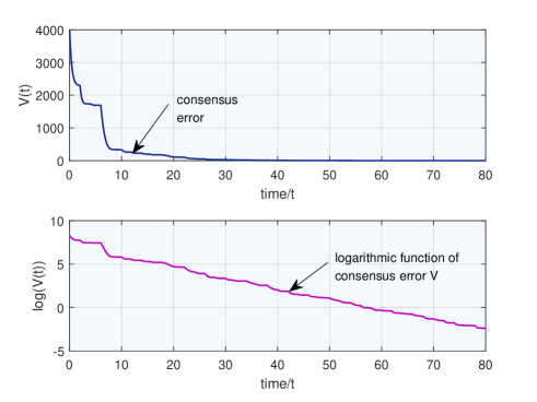
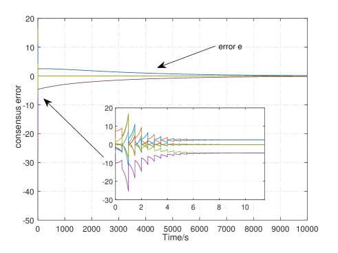
Example 1
In this example, we illustrate Theorem 4 with being neutrally stable. Consider a set of four linear systems interacting with each other. Set
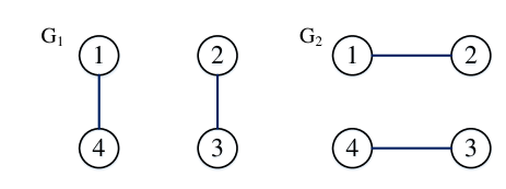
is controllable. Choose the Laplacian matrices (which correspond to two communication graphs and in Fig. 2, respectively) as follows:
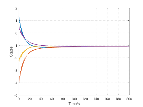
For illustration, the initial values are randomly chosen from . The underlying graph switches every and . Specifically, and for nonnegative integers . Hence, the underlying interaction topology is uniformly jointly connected [28].
By calculation, a positive definite solution of is
To illustrate Theorem 4, note that matrix turns out to be a positive definite solution of the following Riccati equation
| (24) |
where for any and is observable, which is easy to verify. Moreover, does not depend on . Using , a sufficiently small guarantees that the synchronization index is greater than 1.
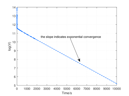
It can be observed from Fig. 1, which plots the logarithmic function of , that the exponential convergence can be guaranteed and the convergence rate is indicated by the slope of the plot.
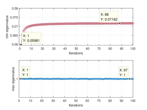
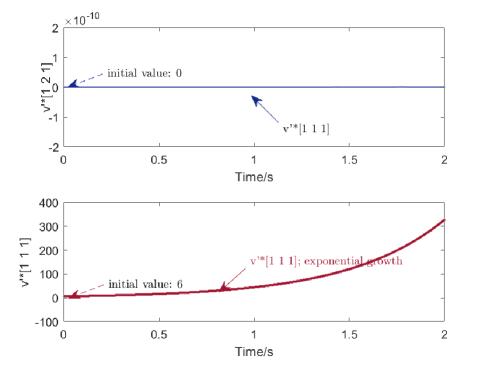
Example 2
We illustrate Theorem 4 with having at least one unstable eigenvalue in this example. Let and for nonnegative integers , where and are shown in Fig. 2. The union of over any time interval of length is connected. Let
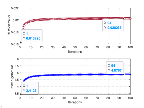
Since is periodic, to perform Algorithm 1 and obtain , one only needs to calculate and with . Via simulation, the maximum and minimum eigenvalues of are, respectively, plotted in Fig. 3. ( is scaled by dividing its largest eigenvalue for ease of illustration.) Evidently, while converges to as . Fig. 4 shows the minimum and the maximum eigenvalues of and with , respectively. It is found that can be chosen as , with which the matrix is
Fig. 5 plots the evolution of with the above , which clearly converges to zero. The convergence rate is implied in Fig. 6 via the slope of .
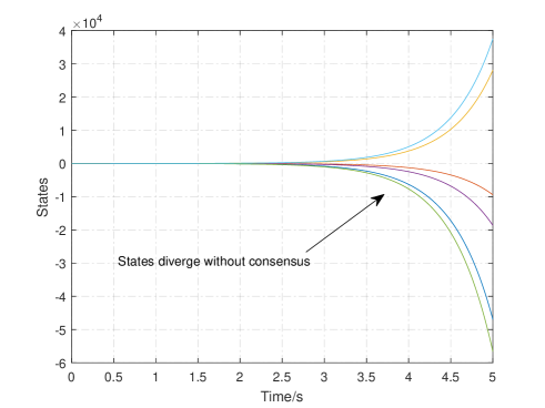
Example 3
In this example, we verify the necessity of controllability of . Consider a matrix pair , which reads
is not controllable with being the uncontrollable eigenvalue. Moreover, spans the uncontrollable space. Choose
and . Consider the same time-varying graph as in Example 1. The evolution of and is shown in Fig. 7, which indicates that consensus cannot be reached. This is also verified in Fig. 8, where the state trajectories clearly depict that no consensus is achieved.
Example 4
In this example, we illustrate the necessity of joint -connectivity for exponential consensus. Let and . Let and be undirected graphs with four nodes and edge weights equal to 1 (see Fig. 9).
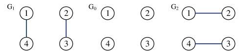
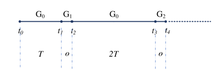
Consider the switching scheme shown in Fig. 10. Specifically, when with , , and where . Note that contains no edge. Recall that is defined in (5).
Moreover, for any given , there exists a such that for , In this example, converges to zero asymptotically as shown in Fig. 11, but not uniformly exponentially fast. To understand why the convergence is not exponential, suppose to the contrary that
for some real numbers and . This implies that there exists an such that for any , a contradiction.
VII Conclusion
In this paper, we have investigated the global uniform exponential consensus problem for controllable linear systems over time-varying undirected networks. A very mild joint connectivity condition on the communication graph has been proposed such that we can construct a set of matrix-valued functions that is precompact. By designing a proper feedback matrix, we have successfully shown that global uniform exponential consensus can be achieved if the joint -connectivity and controllability conditions are satisfied, and in addition a synchronization index is greater than one. The necessity of joint -connectivity and controllability of linear systems for global uniform exponential consensus have also been demonstrated with a properly designed quadratic Lyapunov function candidate. Finally, we point out that being undirected is somewhat restrictive. In view of this, the possible future works include the exploration of symmetric structure underlying a directed switching network topology, by virtue of matrix transformation [46] or group theory [47].
References
- [1] R. Olfati-Saber, J. A. Fax, and R. M. Murray, “Consensus and cooperation in networked multi-agent systems,” Proceedings of the IEEE, vol. 95, no. 1, pp. 215–233, 2007.
- [2] A. Jadbabaie, J. Lin, and A. S. Morse, “Coordination of groups of mobile autonomous agents using nearest neighbor rules,” IEEE Transactions on Automatic Control, vol. 48, no. 6, pp. 988–1001, 2003.
- [3] M. Ye, J. Liu, B. D. O. Anderson, C. Yu, and T. Başar, “Evolution of social power in social networks with dynamic topology,” IEEE Transactions on Automatic Control, vol. 63, no. 11, pp. 3793–3808, 2018.
- [4] J. Qin, Q. Ma, W. X. Zheng, H. Gao, and Y. Kang, “Robust group consensus for interacting clusters of integrator agents,” IEEE Transactions on Automatic control, vol. 62, no. 7, pp. 3559–3566, 2017.
- [5] L. Wang, M. Z. Chen, and Q.-G. Wang, “Bounded synchronization of a heterogeneous complex switched network,” Automatica, vol. 56, pp. 19–24, 2015.
- [6] S. Su and Z. Lin, “Distributed consensus control of multi-agent systems with higher order agent dynamics and dynamically changing directed interaction topologies,” IEEE Transactions on Automatic Control, vol. 61, no. 2, pp. 515–519, 2015.
- [7] F. Xiao, Y. Shi, and W. Ren, “Robustness analysis of asynchronous sampled-data multiagent networks with time-varying delays,” IEEE Transactions on Automatic Control, vol. 63, no. 7, pp. 2145–2152, 2017.
- [8] L. Moreau, “Stability of multiagent systems with time-dependent communication links,” IEEE Transactions on Automatic Control, vol. 50, no. 2, pp. 169–182, 2005.
- [9] P. Wang, G. Wen, T. Huang, W. Yu, and Y. Lv, “Asymptotical neuro-adaptive consensus of multi-agent systems with a high dimensional leader and directed switching topology”, IEEE Transactions on Neural Networks and Learning Systems, DOI: 10.1109/TNNLS.2022.3156279, 2022.
- [10] Y. Zhang and S. Li, “Distributed biased min-consensus with applications to shortest path planning,” IEEE Transactions on Automatic Control, vol. 62, no. 10, pp. 5429–5436, 2017.
- [11] A. Nedic, A. Olshevsky, and W. Shi, “Achieving geometric convergence for distributed optimization over time-varying graphs,” SIAM Journal on Optimization, vol. 27, no. 4, pp. 2597–2633, 2017.
- [12] Y. Chen, S. Kar, and J. M. Moura, “Resilient distributed estimation through adversary detection,” IEEE Transactions on Signal Processing, vol. 66, no. 9, pp. 2455–2469, 2018.
- [13] M. Cao, A. S. Morse, and B. D. O. Anderson, “Reaching a consensus in a dynamically changing environment: convergence rates, measurement delays, and asynchronous events,” SIAM Journal on Control and Optimization, vol. 47, no. 2, pp. 601–623, 2008.
- [14] G. Shi and K. H. Johansson, “The role of persistent graphs in the agreement seeking of social networks,” IEEE Journal on Selected Areas in Communications, vol. 31, no. 9, pp. 595–606, 2013.
- [15] B. D. O. Anderson, G. Shi, and J. Trumpf, “Convergence and state reconstruction of time-varying multi-agent systems from complete observability theory,” IEEE Transactions on Automatic Control, vol. 62, no. 5, pp. 2519–2523, 2016.
- [16] F. Xiao and L. Wang, “Asynchronous consensus in continuous-time multi-agent systems with switching topology and time-varying delays,” IEEE Transactions on Automatic Control, vol. 53, no. 8, pp. 1804–1816, 2008.
- [17] C. Altafini, “Consensus problems on networks with antagonistic interactions,” IEEE Transactions on Automatic Control, vol. 58, no. 4, pp. 935–946, 2012.
- [18] J. Qin, H. Gao, and C. Yu, “On discrete-time convergence for general linear multi-agent systems under dynamic topology,” IEEE Transactions on Automatic Control, vol. 59, no. 4, pp. 1054–1059, 2013.
- [19] T. Yang, Z. Meng, G. Shi, Y. Hong, and K. H. Johansson, “Network synchronization with nonlinear dynamics and switching interactions,” IEEE Transactions on Automatic Control, vol. 61, no. 10, pp. 3103–3108, 2015.
- [20] M. Lu and L. Liu, “Distributed feedforward approach to cooperative output regulation subject to communication delays and switching networks,” IEEE Transactions on Automatic Control, vol. 62, no. 4, pp. 1999–2005, 2016.
- [21] H. Meng, Z. Chen, and R. Middleton, “Consensus of multiagents in switching networks using input-to-state stability of switched systems,” IEEE Transactions on Automatic Control, vol. 63, no. 11, pp. 3964–3971, 2018.
- [22] T. Liu and J. Huang, “Leader-following attitude consensus of multiple rigid body systems subject to jointly connected switching networks,” Automatica, vol. 92, pp. 63–71, 2018.
- [23] Z. Meng, T. Yang, G. Li, W. Ren, and D. Wu, “Synchronization of coupled dynamical systems: Tolerance to weak connectivity and arbitrarily bounded time-varying delays,” IEEE Transactions on Automatic Control, vol. 63, no. 6, pp. 1791–1797, 2017.
- [24] A. Abdessameud, “Consensus of nonidentical euler–lagrange systems under switching directed graphs,” IEEE Transactions on Automatic Control, vol. 64, no. 5, pp. 2108–2114, 2018.
- [25] H. Kim, H. Shim, J. Back, and J. H. Seo, “Consensus of output-coupled linear multi-agent systems under fast switching network: Averaging approach,” Automatica, vol. 49, no. 1, pp. 267–272, 2013.
- [26] J. Back and J.-S. Kim, “Output feedback practical coordinated tracking of uncertain heterogeneous multi-agent systems under switching network topology,” IEEE Transactions on Automatic Control, vol. 62, no. 12, pp. 6399–6406, 2017.
- [27] M. E. Valcher and I. Zorzan, “On the consensus of homogeneous multi-agent systems with arbitrarily switching topology,” Automatica, vol. 84, pp. 79–85, 2017.
- [28] Y. Su and J. Huang, “Stability of a class of linear switching systems with applications to two consensus problems,” IEEE Transactions on Automatic Control, vol. 57, no. 6, pp. 1420–1430, 2012.
- [29] X. Wang, J. Zhu, and J.-e. Feng, “A new characteristic of switching topology and synchronization of linear multiagent systems,” IEEE Transactions on Automatic Control, vol. 64, no. 7, pp. 2697–2711, 2018.
- [30] Q. Ma, J. Qin, W. X. Zheng, Y. Shi, and Y. Kang, “Exponential consensus of linear systems over switching network: A subspace method to establish necessity and sufficiency,” IEEE Transactions on Cybernetics, vol. 52, no. 3, pp. 1565–1574, 2022.
- [31] Q. Ma, J. Qin, X. Yu, and L. Wang, “On necessary and sufficient conditions for exponential consensus in dynamic networks via uniform complete observability theory,” IEEE Transactions on Automatic Control, vol. 66, no. 10, pp. 4975–4981, 2021.
- [32] A. Subramanian, H. Gupta, S. Das, and J. Cao, “Minimum interference channel assignment in multiradio wireless mesh networks,” IEEE Transactions on Mobile Computing, vol. 7, no. 12, pp. 1459–1473, 2008.
- [33] C. Godsil and G. Royle, Algebraic graph theory. Springer, New York, NY, 2001.
- [34] B. D. O. Anderson, “Exponential stability of linear equations arising in adaptive identification,” IEEE Transactions on Automatic Control, vol. 22, no. 1, pp. 83–88, 1977.
- [35] W. Rudin, Principles of mathematical analysis. McGraw-hill New York, 1976, vol. 3.
- [36] J. Simon, “Compact sets in the space ,” Annali di Matematica pura ed applicata, vol. 146, no. 1, pp. 65–96, 1986.
- [37] J. W. Hagood and B. S. Thomson, “Recovering a function from a dini derivative,” The American Mathematical Monthly, vol. 113, no. 1, pp. 34–46, 2006.
- [38] C.-T. Chen, Linear system theory and design. Holt, Rinehart and Winston New York, 1984, vol. 301.
- [39] C.-Q. Ma and J.-F. Zhang, “Necessary and sufficient conditions for consensusability of linear multi-agent systems,” IEEE Transactions on Automatic Control, vol. 55, no. 5, pp. 1263–1268, 2010.
- [40] C. W. Wu, Synchronization in complex networks of nonlinear dynamical systems. World Scientific, 2007.
- [41] R. A. Horn and C. R. Johnson, Matrix Analysis. Cambridge University Press, 2012.
- [42] B. S. Mityagin, “The zero set of a real analytic function,” Matematicheskie Zametki, vol. 107, no. 3, pp. 473–475, 2020.
- [43] H. Marina, “Maneuvering and robustness issues in undirected displacement-consensus-based formation control,” IEEE Trans. Autom. Control, vol. 66, no, 7, pp. 3370–3377, 2021.
- [44] B. Huang, C. Yu, B. D. O. Anderson and G. Mao, “Estimating distances via connectivity in wireless sensor networks, Wirel. Commun. Mob. Comput., vol. 14, pp. 541–556, 2014.
- [45] D. J. Webb and J. Berg, “Kinodynamic RRT*: Asymptotically optimal motion planning for robots with linear dynamics, 2013 IEEE International Conference on Robotics and Automation (ICRA), Karlsruhe, Germany, May 6-10, 2013, pp. 5054–5061.
- [46] J. Qin, H. Gao, and W. X. Zheng, “Exponential synchronization of complex networks of linear systems and nonlinear oscillators: A unified analysis”, IEEE Trans. Neural Netw. Learn. Syst., vol. 26, no. 3, 2015.
- [47] D. Liberzon, J. P. Hespanha, and A. S. Morse, “Stability of switched systems: A Lie-algebraic condition”, Syst. & Control Lett., vol. 37, no. 3, pp. 117-122, 1999.
- [48] H. Khalil, Nonlinear systems third edition. Patience Hall, vol. 115, 2002.
![[Uncaptioned image]](/html/2303.00155/assets/Author_Ma.jpg) |
Qichao Ma received the Ph.D. degree in Control Science and Engineering from University of Science and Technology of China, Hefei, China, in 2019. From 2019 to 2021, he was a Postdoc Researcher with University of Science and Technology of China, Hefei, China, where he is currently a Research Associate Professor. His current research interests include distributed control, decision making, learning, and their applications. |
![[Uncaptioned image]](/html/2303.00155/assets/Author_Qin.jpg) |
Jiahu Qin received the first Ph.D. degree in control science and engineering from Harbin Institute of Technology, Harbin, China, in 2012, and the second Ph.D. degree in systems and control from The Australian National University, Canberra, ACT, Australia, in 2014. He is currently a Professor with the Department of Automation, University of Science and Technology of China, Hefei, China. His current research interests include networked control systems, autonomous intelligent systems, and human-robot interaction. |
![[Uncaptioned image]](/html/2303.00155/assets/Author_Anderson.jpg) |
Brian D. O. Anderson was born in Sydney, Australia, and educated at Sydney University in mathematics and electrical engineering, with PhD in electrical engineering from Stanford University in 1966. He was appointed as ANU’s first engineering professor in 1981. He is now an Emeritus Professor at the Australian National University (having retired as Distinguished Professor in 2016). His awards include the IEEE Control Systems Award of 1997, the 2001 IEEE James H Mulligan, Jr Education Medal, and the Bode Prize of the IEEE Control System Society in 1992, as well as several IEEE and other best paper prizes. He is a Fellow of the Australian Academy of Science, the Australian Academy of Technological Sciences and Engineering, the Royal Society, and a foreign member of the US National Academy of Engineering. He holds honorary doctorates from a number of universities, including Université Catholique de Louvain, Belgium, and ETH, Zürich. He is a past president of the International Federation of Automatic Control and the Australian Academy of Science. |
![[Uncaptioned image]](/html/2303.00155/assets/Author_Wang.jpg) |
Long Wang was born in Xi’an, China. He received the B.E. degree from Tsinghua University, Beijing, in 1986, and the Ph.D. degree from Peking University, Beijing, in 1992, both in dynamics and control. He has held research positions at the University of Toronto, Canada, and the German Aerospace Center, Munich, Germany. He is currently the Cheung Kong Chair Professor of Dynamics and Control, and the Director of Center for Systems and Control of Peking University. His research interests include complex networked systems, evolutionary game dynamics, artificial intelligence, and bio-mimetic robotics. |