Abstract

We consider $10$-dimensional gravitational model with $SO(6)$ Yang-Mills field, Gauss-Bonnet term and $\Lambda$-term. We study so-called cosmological type solutions defined on product manifold $M={\mathbb{R}}\times{\mathbb{R}}^{3}\times K$, where $K$ is $6d$ Calabi-Yau manifold. By putting the gauge field 1-form to be coinciding with 1-form spin connection on $K$, we obtain exact cosmological solutions with exponential dependence of scale factors (upon $t$-variable), governed by two non-coinciding Hubble-like parameters: $H>0$, $h$, obeying $H+2h\neq 0$. We also present static analogs of these cosmological solutions (for $H\neq 0$, $h\neq H$ and $H+2h\neq 0$). The islands of stability for both classes of solutions are outlined.

Key words: cosmology; Gauss-Bonnet; Calabi-Yau; Yang-Mills; stability; exact solutions

1 Introduction

Here we deal with a so-called Einstein-Gauss-Bonnet-Yang-Mills-$\Lambda$ gravitational model in dimension $D=10$. The action of the model contains scalar curvature, Gauss-Bonnet, cosmological term ($\Lambda$-term) and Yang-Mills term with a value in $so(6)$ Lie algebra. The model includes non-zero constant $\alpha$, coupled to the sum of Yang-Mills and Gauss-Bonnet terms. The equations of motion for this model are of second order (like it takes place in General Relativity). The so-called Gauss-Bonnet term has appeared in (super)string theory as a second order correction in curvature to the effective (super)string effective action [1, 2, 3] for a heterotic string [4].

At present, Einstein-Gauss-Bonnet (EGB) gravitational models, e.g. with cosmological term and extra matter fields and its modifications [5]-[26], are under intensive studyies in astrophysics and cosmology. The main goal in these studies is a solution of dark energy problem. One can study such models for possible explanation of accelerating expansion of the Universe, which was supported by supernovae (type Ia) observational data [27, 28].

We note that at present there exist several modifications of Einstein and EGB actions which correspond to $F(R)$, $R+f({\cal G})$, $f({R,\cal G})$, $f({R,\cal G})$ , $f({R,\cal G},T_{..}T^{..})$ theories (e.g. for $D=4$), where $R$ is scalar curvature and ${\cal G}$ is Gauss-Bonnet term. These modifications are under intensive studying devoted to cosmological, astrophysical and other applications, see [29]-[35] and references therein.

Another point of interest is a search of possible local manifestation of dark energy related to wormholes, black holes, etc. The most important results for black holes in models with Gauss-Bonnet term are related with the Boulware-Deser-Wheeler solution [36, 37] and its generalizations [38, 39, 40, 41], see also Refs. [42, 43, 44] and references therein. For certain applications of brane-world models with Gauss-Bonnet term, see Refs. [45, 46] and related bibliography. For wormholes solutions in Einstein-Gauss-Bonnet models with certain fields see Refs. [47, 48] and references threin.

In this article we deal with the so-called cosmological type solutions with the $10d$ metric

$$g^{(10)}=-wd\chi\otimes d\chi+a^{2}_{3}(\chi)g^{(3)}+a^{2}_{6}(\chi)g^{(6)}.$$ (1.1)

defined on product manifold ${\mathbb{R}}\times{\mathbb{R}}^{3}\times K,$ where $w=\pm 1$, ${\mathbb{R}}^{3}$ is flat $3d$ manifold (“our” space) with the metric $g^{(3)}$ and $K$ is $6d$ Ricci-flat Calabi-Yau manifold (internal space) of $SU(3)$ holonomy group with the metric $g^{(6)}$. The warped product model is governed by two scale factors, depending upon one variable $\chi$. It is the synchronous time variable for cosmological case $w=1$: $\chi=t$, while it coincides with space-like variable for $w=-1$: $\chi=u$. The presence of Yang-Mills field makes this ansatz consistent if we choose the Lie algebra for Yang-Mills field to be equal (at least) to $so(6)$, which contains $su(3)$ subalgebra, corresponding to $SU(3)$ group of golonomy of $6d$ Calabi-Yau manifold. For Yang-Mills field we consider the following ansatz: we put here the gauge field 1-form to be equal to spin connection 1-form on $K$ (see Section 2): $A=\omega^{(6)}$. In such ansatz the gauge field plays a role of compensator which “waves out” the terms with non-zero Riemann tensor of Calabi-Yau metric $g^{(6)}$.

Originally such idea of compensation was used by Wu and Wang [49] (see also [50]) in $(1+3+6)$-dimensional cosmological model based on $10d$ Yang-Mills ($SO(32)$- and/or $E_{8}\times E_{8}$-) supergravity theory “upgrated” by additions of Chern-Simons and Gauss-Bonnet terms (of superstring origin). The work of Wu and Wang was influenced greatly by the well-known paper of Candelas et al. [51] devoted to vacuum configurations in ten-dimensional $O(32)$ and $E_{8}\times E_{8}$ supergravity and superstring theory that have unbroken $N=1$ supersymmetry in four dimensions.

It should be noted that compactifications of $11$-dimensional supergravity on ($6d$) Calabi-Yau manifold were considered in Refs. [52, 53]. Moreover, $4d$ and $6d$ Calabi-Yau manifolds also appeared in partially sypersymmetric solutions of $D=11$ supergravity with $M$-branes, see Refs. [54, 55, 56] and and references threin.

In Section 3 we obtain exact cosmological solutions with exponential dependence of scale factors (upon $t$-variable), governed by two non-coinciding Hubble-like parameters: $H>0$ and $h$, corresponding to factor spaces of dimensions $3$ and $6$, respectively, when the following restriction $3H+6h\neq 0$ is used (excluding the solutions with constant volume factor).

In Section 4 we obtain static solutions ($w=-1$) for non-coinciding Hubble parameters $H\neq 0$, $h$, which obey $3H+6h\neq 0$. We also study stability (in certain restricted sence) of the obtained solutions in cosmological case for $t\to+\infty$ (see Section 3) and in static case for $u\to\pm\infty$ (see Section 4) by using results of Ref. [22] (see also approach of Ref. [19]) and single out the subclasses of stable/non-stable solutions.

2 The $10$-dimensional model

2.1 The action and equations of motion

We take the action of the model as

$$S=\frac{1}{2\kappa^{2}}\int d^{10}x\sqrt{-g}\left\{R+\alpha\left[{\rm tr}F_{MN}F^{MN}\right.\right.$$

$$\left.\left.+R_{MNPQ}R^{MNPQ}-4R_{MN}R^{MN}+R^{2}\right]\right\},$$ (2.1)

where $\kappa^{2}$ is $10$-dimensional gravitational constant, $\alpha\neq 0$ is constant, $g_{MN}$ are components of the metric, $F_{MN}$ are components of the Yang-Mills field strengths corresponding to $2$-form with the value in the Lie algebrs $so(6)$: $F=\frac{1}{2}F_{MN}dx^{M}\wedge dx^{N}=dA+A\wedge A,$ where $A=A_{M}dx^{M}$ is the $1$-form with the value in $so(6)$ ($F_{MN}=\partial_{M}A_{N}-\partial_{N}A_{M}+[A_{M},A_{N}]$).

The action (2.1) leads us to the following equations of motions:

$$R_{MN}-\frac{1}{2}g_{MN}R=-2\alpha\biggl{(}{\rm tr}F_{MP}F_{N}^{\ \ P}-\frac{1}{4}g_{MN}\ {\rm tr}F_{PQ}F^{PQ}\biggr{)}\qquad\qquad$$

$$+\alpha\biggl{[}\frac{1}{2}g_{MN}(R_{MNPQ}R^{MNPQ}-4R_{MN}R^{MN}+R^{2})-2RR_{MN}$$

$$+4R_{MP}R_{N}^{\ \ P}+4R_{MPNQ}R^{PQ}-2R_{M}^{\ \ PQS}R_{NPQS}\biggr{]},$$ (2.2)

$$D_{M}F^{MP}=0.$$ (2.3)

Here we use notation for covariant gauge derivative: $D_{M}=D_{M}(A)=\nabla_{M}+[A_{M},.]$.

2.2 Cosmological ansatz.

Let us consider ten-dimensional manifold

$$M={\mathbb{R}}\times{\mathbb{R}}^{3}\times K,$$ (2.4)

where $K$ is a $6d$ Calabi-Yau manifold, i.e., a compact 6-dimensional Kähler Ricci-flat manifold with the metric, which has $SU(3)$ holonomy group. For corresponding Lie algebra we have $su(3)\subset so(6)$.

We start with the cosmological case, i.e. we consider the set of equations (2.2), (2.3) on the manifold (2.4) with the following ansatz for fields

$$g^{(10)}=-dt\otimes dt+a^{2}_{3}(t)g^{(3)}+a^{2}_{6}(t)g^{(6)},$$ (2.5)

$$A=\omega^{(6)}.$$ (2.6)

Here $g^{(3)}=dx^{1}\otimes dx^{1}+dx^{2}\otimes dx^{2}+dx^{3}\otimes dx^{3}$, i.e. we deal with a flat Euclidean metric on ${\mathbb{R}}^{3}$ and $g^{(6)}=g^{(6)}_{mn}(y)dy^{m}\otimes dy^{n}$ is Calabi-Yau metric on $K$.

By $\omega^{(6)}=\omega^{(6)}_{m}(y)dy^{m}$ we denote the spin connection 1-form on $K$ with the value in the Lie algebra $so(6)$ corresponding to the (local) basis of co-vectors $e^{a}_{\ m}$ on $K$ , which diagonalizes the metric $g^{(6)}$:

$$g^{(6)}_{mn}=e^{a}_{\ m}e^{b}_{\ n}\delta_{ab},$$ (2.7)

$$\omega^{(6)}_{m}=\mid\mid\omega^{(6)a}_{\ \ \ \ bm}\mid\mid\equiv\mid\mid e^{a}_{\ n}\nabla^{(6)}_{m}e^{n}_{\ b}\mid\mid\subset so(6),$$ (2.8)

where covariant derivative $\nabla^{(6)}_{m}$ corresponds to the metric $g^{(6)}$ and $e^{n}_{\ b}$ is “inverse” (dual) basis of vector fields obeying $e^{a}_{\ n}e^{n}_{\ b}=\delta^{a}_{b}$.

It follows from (2.6) that

$$F=\Omega^{(6)},$$ (2.9)

where $\Omega^{(6)}=d\omega^{(6)}+\omega^{(6)}\wedge\omega^{(6)}$ is the curvature two-form on $K$ with the value in $so(6)$.

The spin connection $\omega^{(6)}$ on $K$ obeys the identity

$$D_{m}(\omega^{(6)})\Omega^{(6)mn}=0,$$ (2.10)

where $D_{m}(\omega^{(6)})=\nabla^{(6)}_{m}+[\omega^{(6)}_{m},.\ ]$. The identity (2.10) is equivalent to the following identity for the Riemann tensor on $K$

$$\nabla^{(6)}_{m}R^{(6)mnpq}=0,$$ (2.11)

which is valid for any Kähler Ricci-flat manifold [57].

The Yang-Mills equations (2.3) are satisfied identically due to eqs. (2.5), (2.6) and (2.10).

Let us denote

$$H(t)\equiv\dot{a}_{3}/a_{3},\qquad h(t)\equiv\dot{a}_{6}/a_{6},$$ (2.12)

where in this section we denote $\dot{a}\equiv\frac{da}{dt}$.

Then, equations (2.2) for the ansatz (2.5)-(2.6) may be written as follows:

$$B_{0}+2\Lambda-\alpha B_{1}=0,$$ (2.13)

$$\frac{dL_{H}}{dt}+(3H+6h)L_{H}-L_{0}=0,$$ (2.14)

$$\frac{dL_{h}}{dt}+(3H+6h)L_{h}-L_{0}=0.$$ (2.15)

Here

$$L_{0}=B_{0}-2\Lambda-\frac{1}{3}\alpha B_{1},$$ (2.16)

$$L_{H}=2B_{H}-\frac{4}{3}\alpha A_{H},$$ (2.17)

$$L_{h}=2B_{h}-\frac{4}{3}\alpha A_{h},$$ (2.18)

$$B_{0}=3H^{2}+6h^{2}-(3H+6h)^{2},$$ (2.19)

$$\quad B_{H}=H-(3H+6h),$$ (2.20)

$$\quad B_{h}=h-(3H+6h),$$ (2.21)

$$B_{1}=144H^{3}h+1080H^{2}h^{2}+1440Hh^{3}+360h^{4}$$ (2.22)

and

$$A_{H}=36H^{2}h+180Hh^{2}+120h^{3},$$ (2.23)

$$A_{h}=6H^{3}+90H^{2}h+180Hh^{2}+60h^{3}.$$ (2.24)

Equations (2.13)-(2.15) are obtained from (2.2) using the Ricci flatness of $K$ and the equality for Riemann tensor of internal space $K$ with the metric $g^{(6)}$

$$R^{(6)}_{pqmn}R^{(6)qp^{\prime}mn}=g^{(6)mp^{\prime}}g^{(6)nq}\ {\rm tr}\ F_{mn}F_{pq},$$ (2.25)

which follows from (2.9) and well-known identity

$$R^{(6)p}_{\ \ \ \ qmn}=e^{p}_{\ a}\ e^{b}_{\ q}\ \Omega^{(6)a}_{\ \ \ \ bmn}\ .$$ (2.26)

3 Cosmological solutions

Here we consider the case when Hubble-like parameters are constant, i.e.

$$H(t)=H={\rm const},\qquad h(t)=h={\rm const}.$$ (3.1)

For scale factors we get the exponential dependence on $t$

$$a_{3}(t)=\exp(Ht),\qquad a_{6}(t)=\exp(ht).$$ (3.2)

We get a set of polynomial equations

$$B_{0}+2\Lambda-\alpha B_{1}=0,$$ (3.3)

$$(3H+6h)L_{H}-L_{0}=0,$$ (3.4)

$$(3H+6h)L_{h}-L_{0}=0,$$ (3.5)

where polynomials $B_{0},B_{1},L_{0},L_{H},L_{h}$ are defined above.

We set

$$H>0.$$ (3.6)

This relation is used for a description of an accelerated expansion of the $3$-dimensional subspace (which may describe our Universe). The evolution of the $6$-dimensional internal factor space is described by the Hubble-like parameter $h$.

It follows from Ref. [22, 24] (for a more general splitting scheme see paper by Chirkov, Pavluchenko and Toporensky [18]) that if we consider Hubble-like parameters $H$ and $h$ obeying two restrictions imposed

$$3H+6h\neq 0,\qquad H\neq h,$$ (3.7)

we reduce relations (3.3), (3.4), (3.5) to the following set of equations

$$E=3H^{2}+6h^{2}-(3H+6h)^{2}+2\Lambda\qquad$$

$$-\alpha[144H^{3}h+1080H^{2}h^{2}+1440Hh^{3}+360h^{4}]=0,$$ (3.8)

$$Q=2H^{2}+20Hh+20h^{2}=-\frac{1}{2\alpha}.$$ (3.9)

Using equation (3.9), we get

$$H=(-2\alpha{\cal P})^{-1/2},$$ (3.10)

where

$${\cal P}={\cal P}(x)\equiv 2+20x+20x^{2},$$ (3.11)

$$x\equiv h/H,$$ (3.12)

and

$$\alpha{\cal P}<0.$$ (3.13)

Due to restrictions (3.7) we have for $x$ from (3.12)

$$x\neq x_{d}\equiv-1/2,\qquad x\neq x_{a}\equiv 1.$$ (3.14)

The relation (3.9) is valid only if

$${\cal P}(x)\neq 0.$$ (3.15)

Substituting relation (3.10) into (3.8) we obtain

$$\Lambda\alpha\equiv\lambda=f(x)\equiv(1/4)[3+6x^{2}-(3+6x)^{2}](2+20x+20x^{2})^{-1}$$

$$+(1/8)[18(8x+60x^{2}+80x^{3}+20x^{4})](2+20x+20x^{2})^{-2}.$$ (3.16)

From (3.15) we get

$$x\neq x_{\pm}\equiv\frac{-10\pm\sqrt{10}}{20},$$ (3.17)

where $x_{\pm}$ are roots of the quadratic equation ${\cal P}(x)=0$. They obey

$$x_{-}<x_{+}<0.\qquad$$ (3.18)

According to eq. (3.13) we get (in this cosmological case)

$$x_{-}<x<x_{+}\ \ {\rm for}\ \alpha>0,\qquad$$ (3.19)

and

$$x<x_{-}\ {\rm or}\ x>x_{+}\ \ {\rm for}\ \alpha<0.\qquad$$ (3.20)

The graphical representation of the function $\lambda=f(x)$ is given at Figure 1.

The function $f(x)$ obeys

$$\lim_{x\to\pm\infty}f(x)=\lambda_{\infty}\equiv-\frac{21}{80}\qquad$$ (3.21)

and

$$\lim_{x\to x_{\pm}}f(x)=-\infty.\qquad$$ (3.22)

It has a maximum at $x_{c}=-\frac{1}{5}$ with the value $f(x_{c})=\lambda_{c}\equiv 3/10$ and an inflection point at $x_{d}=-\frac{1}{2}$ with the value $f(x_{d})=\lambda_{d}\equiv 3/16$. It has also a point of local maximum at $x_{a}\equiv 1$ with the value $f(x_{a})=\lambda_{a}\equiv-3/14$.

Equation (3.16) is equivalent to the following master equation

$$(400\lambda+105)x^{4}+(800\lambda+150)x^{3}+(480\lambda+90)x^{2}+(80\lambda+30)x+4\lambda+3=0.$$ (3.23)

For

$$\lambda\neq\lambda_{\infty}\equiv-21/80$$ (3.24)

the solution to this (fourth order) master equation reads

$$x=\varepsilon_{1}\frac{1}{2}\sqrt{-\frac{\varepsilon_{2}A}{\sqrt{X}}-Y^{1/3}+BY^{-1/3}+C}$$

$$-\varepsilon_{2}\frac{\sqrt{X}}{2\sqrt{5}(80\lambda+21)}-\frac{5(16\lambda+3)}{2(80\lambda+21)},$$ (3.25)

where $\varepsilon_{1}=\pm 1$, $\varepsilon_{2}=\pm 1$,

$$A=(18\sqrt{5}(1280\lambda^{2}+96\lambda-39))/(80\lambda+21)^{2},$$ (3.26)

$$B=-(4(16\lambda-3)(20\lambda+3))/(5(80\lambda+21)^{2}),$$ (3.27)

$$C=(2(16\lambda+3)(80\lambda-9))/(80\lambda+21)^{2},$$ (3.28)

and

$$X=5(80\lambda+21)^{2}Y^{1/3}+5(16\lambda+3)(80\lambda-9)+4(16\lambda-3)(20\lambda+3)Y^{-1/3},$$ (3.29)

$$Y=(36(16\lambda-3)\sqrt{-(10\lambda-3)(14\lambda+3)})/(5^{3/2}(80\lambda+21)^{3})+Z,$$ (3.30)

$$Z=(4(16\lambda-3)(320\lambda^{2}+42\lambda-9))/(5(80\lambda+21)^{3}).$$ (3.31)

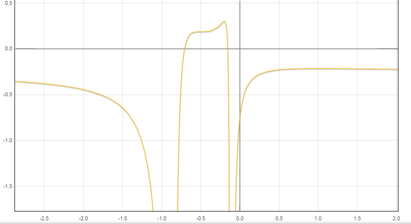
Figure 1: The graphical representation of moduli function $\lambda=f(x)$ given by relation (3.16).

It follows from Figure 1 that for given parameters $\Lambda$ and $\alpha$, obeying restrictions $\alpha\neq 0$ and (3.24), real solutions in formula (3.25) appear for suitably chosen $\varepsilon_{1}=\pm 1$ and $\varepsilon_{2}=\pm 1$ if

$$\lambda=\Lambda\alpha\leq\lambda_{c}=3/10$$ (3.32)

for $\alpha>0$ and

$$\lambda=\Lambda\alpha<\lambda_{a}=-3/14$$ (3.33)

for $\alpha<0$.

For example, for $\lambda=\lambda_{c}=3/10$ relation (3.25) gives us $x=x_{c}=-1/5$ if we put $\varepsilon_{1}=\pm 1$ and $\varepsilon_{2}=-1$.

In exceptional case

$$\lambda=\lambda_{\infty}=-21/80$$ (3.34)

we have a cubic master equation (3.23) which has three real roots

$$x=x_{k}=(1/10)(-2-6\cos{(\theta/3+2k\pi/3)}),\qquad\tan{\theta}=\sqrt{15},$$ (3.35)

$k=1,2,3$, or, numerically

$$x_{1}\approx 0.29253505115,\quad x_{2}\approx-0.14952367803,\quad x_{3}\approx-0.74301143583.$$ (3.36)

Graphical analysis. The graphical representation $\Lambda|\alpha|$ upon $x=h/H$ (in this cosmological case) is presented at Figure 2. In drawing this figure we use the relation

$$\Lambda|\alpha|=\lambda{\rm sgn}(\alpha)=f(x)\frac{(-2-20x-20x^{2})}{|2+20x+20x^{2}|},$$ (3.37)

in agreement with (3.11) and (3.13). It follows from Figure 2 that real solutions take place if

$$\Lambda|\alpha|\leq\lambda_{c}=3/10,$$ (3.38)

for $\alpha>0$ and

$$\Lambda|\alpha|>|\lambda_{a}|=3/14,$$ (3.39)

for $\alpha<0$. (The point $x_{a}=1$ is excluded from our consideration.)

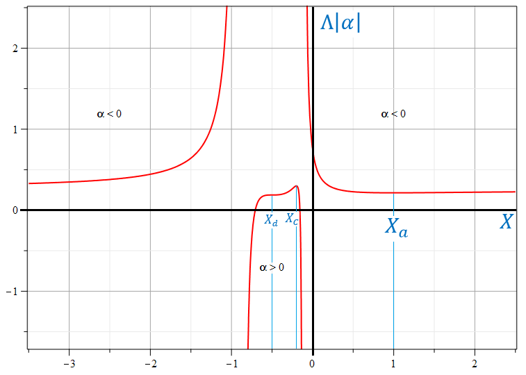
Figure 2: The dependence of $\Lambda|\alpha|$ upon $x=h/H$ in cosmological case. The central branch coresponds to $\alpha>0$. The left and right branches corespond to $\alpha<0$.

Stability.

Using results of Ref. [22, 24] we obtain that cosmological solutions under consideration obeying $x=h/H\neq x_{i}$, $i=a,c,d$, where $x_{a}=1$, $x_{c}=-\frac{1}{5}$, $x_{d}=-\frac{1}{2}$, are stable if i) $x>x_{d}=-1/2$ and unstable if ii) $x<x_{d}=-1/2$.

We note that the the points $x_{a}=1$ and $x_{d}=-1/2$ are excluded from our consideration due to restrictions (3.7) while the point of maximum $x_{c}=-\frac{1}{5}$ is excluded since the analysis of Ref. [22] was based on the equations for perturbations for $\delta H(t)$, $\delta h(t)$ in the linear approximation which can be resolved when $x_{c}\neq-\frac{1}{5}$. In special case $x_{c}=-\frac{1}{5}$ higher order terms in pertubations should be considered.

Let us denote by $n_{s}$ the number of non-special stable solutions. By using Figure 2 we find just graphically for $\alpha>0$

$$n_{s}=\begin{cases}0,\ \Lambda\alpha\geq\lambda_{c}=3/10,\\ 2,\ \lambda_{d}=3/16<\Lambda\alpha<\lambda_{c}=3/10,\\ 1,\ \Lambda\alpha\leq\lambda_{d}=3/16.\\ \end{cases}$$ (3.40)

(here $\lambda_{i}=f(x_{i})$) while for $\alpha<0$ we obtain

$$n_{s}=\begin{cases}1,\ \Lambda|\alpha|\geq|\lambda_{\infty}|=21/80,\\ 2,\ |\lambda_{a}|=3/14<\Lambda|\alpha|<|\lambda_{\infty}|=21/80,\\ 0,\ \Lambda|\alpha|\leq|\lambda_{a}|=3/14.\\ \end{cases}$$ (3.41)

Thus, for $\alpha>0$ and small enough value of $\Lambda$ there exists at least one stable solution with $x\in(x_{-},x_{+})$, while for $\alpha<0$ and big enough value of $\Lambda$ there exists at least one stable solution with $x$ obeying $x>x_{+}$. The solutions with $x<x_{-}$ are unstable.

In cosmological case real solutions corresponding to $\Lambda=0$ exists only if $\alpha>0$. We obtain from (3.25) for $\varepsilon_{1}=\pm 1$, $\varepsilon_{2}=1$, two solutions

$$x_{-}\approx-0.70692427923,\qquad x_{+}\approx-0.15626295995.$$ (3.42)

The first cosmological solution (for $x_{-}$) is unstable, while the second one (for $x_{+}$) is stable in agreement with Ref. [25].

Remark. It should be noted that here as in the Ref. [22] we deal with restricted stability problem. We do not consider the general setup for perturbations $\delta g_{MN}(t,x)$ and $\delta A_{M}(t,x)$ but only consider the cosmological perturbations of scale factors $\delta a_{3}(t)$, $\delta a_{6}(t)$ in the framework of our ansatz (2.5), (2.6) with fixed $g^{(10)}$ and $\omega^{(6)}$. Analogous remark should be addressed to our analysis of static solutions in the next section.

Zero variation of $G$. The cosmological solution with $x=0$, or $h=0$, takes place if $\alpha<0$ and

$$\Lambda\alpha=-3/4.$$ (3.43)

We get $\Lambda>0$. The scale factor $a_{6}$ is constant in this case and we are led to zero variation of the effective $4d$ gravitational constant (in Jordan frame). This solution is stable. Moreover, we get $H^{2}=-1/(4\alpha)$, which implies for the effective $4$-dimensional cosmological constant $\Lambda_{eff}=3H^{2}=\Lambda$. In general case $\Lambda_{eff}$ is a nontrivial function of $\Lambda$ and $\alpha$ given by (3.10) and generic solution for $x$ from (3.25) (or from (3.35) in special case).

We note that for $\alpha<0$ and for $\Lambda$ from (3.43) there exists another real solution corresponding to certain $x_{*}<x_{-}$, which is unstable.

4 Static analogs of cosmological solutions

Now with deal with the static case by considering the set of equations (2.2), (2.3) on the manifold (2.4) with the following ansatz

$$g^{(10)}=du\otimes du+a^{2}_{3}(u)g^{(3)}+a^{2}_{6}(u)g^{(6)},$$ (4.1)

$$A=\omega^{(6)},$$ (4.2)

where $u$ is a spatial coordinate and $g^{(3)}=-dt\otimes dt+dx^{1}\otimes dx^{1}+dx^{2}\otimes dx^{2},$ is flat pseudo-Eucleadean metric on ${\mathbb{R}}^{3}$, $g^{(6)}$ is the Calabi-Yau metric on $K$ and $\omega^{(6)}$ is spin connection 1-form on $K$ defined in a previous section.

The Yang-Mills equations are satisfied identically as in the previous case.

Now, we denote

$$H(u)\equiv\dot{a}_{3}/a_{3},\qquad h(u)\equiv\dot{a}_{6}/a_{6},$$ (4.3)

where in this section we denote $\dot{a}\equiv\frac{da}{du}$.

Then, equations (2.2) in the ansatz (4.1)-(4.2) may be written as follows:

$$B_{0}-2\Lambda+\alpha B_{1}=0,$$ (4.4)

$$\frac{d\bar{L}_{H}}{du}+(3H+6h)\bar{L}_{H}-L_{0}=0,$$ (4.5)

$$\frac{d\bar{L}_{h}}{du}+(3H+6h)\bar{L}_{h}-L_{0}=0,$$ (4.6)

where

$$\bar{L}_{0}=B_{0}+2\Lambda+\frac{1}{3}\alpha B_{1},$$ (4.7)

$$\bar{L}_{H}=2B_{H}+\frac{4}{3}\alpha A_{H},$$ (4.8)

$$\bar{L}_{h}=2B_{h}+\frac{4}{3}\alpha A_{h},$$ (4.9)

$B_{0},B_{H},B_{h},B_{1}$ are defined in (2.19), (2.20), (2.21), (2.22), and $A_{H},A_{h}$ are defined in (2.23), (2.24), respectively.

As we see, the equations of motion for “Hubble-like” parameters (4.3) in static case may be obtained from cosmological ones (of Section 3) just by replacement

$$\alpha\mapsto-\alpha,\qquad\Lambda\mapsto-\Lambda.$$ (4.10)

The dimensionless parameter $\lambda=\Lambda\alpha$ is invariant under this replacement.

Here we consider the case when “Hubble-like” parameters are constant, i.e.

$$H(u)=H={\rm const},\qquad h(u)=h={\rm const},$$ (4.11)

or, equivalently,

$$a_{3}(u)=\exp(Hu),\qquad a_{6}(u)=\exp(hu).$$ (4.12)

We get a set of polynomial equations

$$B_{0}-2\Lambda+\alpha B_{1}=0,$$ (4.13)

$$(3H+6h)\bar{L}_{H}-\bar{L}_{0}=0,$$ (4.14)

$$(3H+6h)\bar{L}_{h}-\bar{L}_{0}=0,$$ (4.15)

where polynomials $\bar{L}_{0},\bar{L}_{H},\bar{L}_{h}$ are defined by relations (4.7), (4.8), (4.9), respectively.

Here we consider slightly more general case

$$H\neq 0.$$ (4.16)

As in previous section we impose the conditions (3.7) and reduce relations (4.13), (4.14), (4.15) to the set of two equations [26]

$$\bar{E}=3H^{2}+6h^{2}-(3H+6h)^{2}-2\Lambda\qquad$$

$$+\alpha[144H^{3}h+1080H^{2}h^{2}+1440Hh^{3}+360h^{4}]=0,$$ (4.17)

$$Q=2H^{2}+20Hh+20h^{2}=\frac{1}{2\alpha}.$$ (4.18)

Using equation (4.18) and restriction (4.16) we get

$$H=\varepsilon_{0}(2\alpha{\cal P})^{-1/2},$$ (4.19)

where $\varepsilon_{0}=\pm 1$, and quadratic polynomial ${\cal P}={\cal P}(x)$ ($x=h/H$) is defined in (3.11).

Here we get

$$\alpha{\cal P}>0,$$ (4.20)

instead of (3.13).

According to eq. (4.20) we get in the static case

$$x_{-}<x<x_{+}\ \ {\rm for}\ \alpha<0,\qquad$$ (4.21)

and

$$x<x_{-}\ {\rm or}\ x>x_{+}\ \ {\rm for}\ \alpha>0.\qquad$$ (4.22)

(The real numbers $x_{\pm}$ are defined in (3.17).)

We obtain that the main equations (3.16) and (3.23) for the ratio $x=h/H$ are unchanged in static case.

Thus, for $\lambda\neq-21/80$ and restrictions (3.7), (4.16) imposed, we obtain exact solutions for $H$ and $h$, which are given by formulae (3.25), (4.19) and (4.20). For $\lambda=-21/80$ we should use (3.35) instead of (3.25).

Graphical analysis. The graphical representation of $\Lambda|\alpha|$ upon $x=h/H$ in the static case is presented at Figure 3. Here we use the relation

$$\Lambda|\alpha|=\lambda{\rm sgn}(\alpha)=f(x)\frac{(2+20x+20x^{2})}{|2+20x+20x^{2}|},$$ (4.23)

in agreement with (4.20). It follows from Figure 3 that real solutions take place if

$$\Lambda|\alpha|\geq-\lambda_{c}=-3/10,$$ (4.24)

for $\alpha<0$ and

$$\Lambda|\alpha|<\lambda_{a}=-3/14,$$ (4.25)

for $\alpha>0$.

In static case real solutions for $\Lambda=0$ exists only if $\alpha<0$.

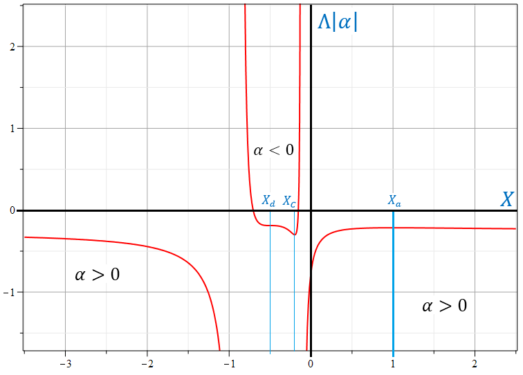
Figure 3: The dependence of $\Lambda|\alpha|$ upon $x=h/H$ in static case. The central branch coresponds to $\alpha<0$. The left and right branches corespond to $\alpha>0$.

Stability.

Using results of Ref. [26] we can analyse the stability of static solutions under consideration obeying $x=h/H\neq x_{i}$, $i=a,c,d$, where $x_{a}=1$, $x_{c}=-\frac{1}{5}$, $x_{d}=-\frac{1}{2}$.

The solutions are stable for $H>0$ and $u\to+\infty$ if i) $x>x_{d}=-1/2$ and unstable if ii) $x<x_{d}=-1/2$. For $H>0$ and $u\to-\infty$ they stable for i) $x<x_{d}=-1/2$ and unstable if ii) $x>x_{d}=-1/2$.

The solutions are stable for $H<0$ and $u\to+\infty$ if i) $x<x_{d}=-1/2$ and unstable if ii) $x>x_{d}=-1/2$. For $H<0$ and $u\to-\infty$ they stable for i) $x>x_{d}=-1/2$ and unstable if ii) $x<x_{d}=-1/2$.

5 Conclusions

Here we have considered Einstein-Gauss-Bonnet-Yang-Mills-$\Lambda$ gravitational model in dimension $D=10$ with non-zero constant $\alpha$ coupled to a sum of Yang-Mills and Gauss-Bonnet terms.

We have studied so-called cosmological type solutions with the metrics (1.1) defined on product manifolds $M={\mathbb{R}}\times{\mathbb{R}}^{3}\times K$, where $w=\pm 1$, ${\mathbb{R}}^{3}$ is flat $3d$ subspace with the metric $g^{(3)}$, and $K$ is $6d$ Ricci-flat Calabi-Yau manifold with the metric $g^{(6)}$. The gauge field 1-form was considered to be coinciding with spin connection 1-form on $K$: $A=\omega^{(6)}$.

For $w=+1$, $\chi=t$, we have obtained exact cosmological solutions with exponential dependence of scale factors (upon $t$-variable), governed by two non-coinciding Hubble-like parameters: $H>0$, $h$, corresponding to factor spaces of dimensions $3$ and $6$, respectively, when the following restriction: $3H+6h\neq 0$ is used (excluding the solutions with constant volume factor).

Static analogs of cosmological solutions ($w=-1$, $\chi=u$ ) with exponential dependence of scale factors and non-coinciding “Hubble-like” parameters $H\neq 0$ and $h$, obeying $3H+6h\neq 0$, are also presented here.

We have also outlined the stability of the solutions in cosmological case (for $t\to+\infty$, Section 3) and in static case for ($u\to\pm\infty$, Section 4) and have singled out “islands” of stable/non-stable solutions.

Some cosmological applications of the model ($w=1$) may be of interest in context of dark energy problem and problems of stability/variation of gravitational constant. For static case ($w=-1$) possible applications of the obtained solutions may be a subject of a further research, aimed at a search of topological black hole solutions (with flat horizon) or wormhole solutions which are coinciding asymptotically (for $u\to\pm\infty$) with our solutions.

Acknowledgments

This research was funded by RUDN University, scientific project number FSSF-2023-0003.

References

- [1] B. Zwiebach, Curvature squared terms and string theories, Phys. Lett. B 156, 315 (1985).
- [2] E.S. Fradkin and A.A. Tseytlin, Effective action approach to superstring theory, Phys. Lett. B 160, 69-76 (1985).
- [3] D. Gross and E. Witten, Superstrings modifications of Einstein’s equations, Nucl. Phys. B 277, 1 (1986).
- [4] D.J. Gross, J.A. Harvey, E. Martinec and R. Rohm, Heterotic String, Phys. Rev. Lett. 54, 502 (1984).
- [5] H. Ishihara, Cosmological solutions of the extended Einstein gravity with the Gauss-Bonnet term, Phys. Lett. B 179, 217 (1986).
- [6] N. Deruelle, On the approach to the cosmological singularity in quadratic theories of gravity: the Kasner regimes, Nucl. Phys. B 327, 253-266 (1989).
- [7] S. Nojiri and S.D. Odintsov, Introduction to modified gravity and gravitational alternative for Dark Energy, Int. J. Geom. Meth. Mod. Phys. 4, 115-146 (2007); hep-th/0601213.
- [8] E. Elizalde, A.N. Makarenko, V.V. Obukhov, K.E. Osetrin and A.E. Filippov, Stationary vs. singular points in an accelerating FRW cosmology derived from six-dimensional Einstein-Gauss-Bonnet gravity, Phys. Lett. B 644, 1-6 (2007); hep-th/0611213.
- [9] K. Bamba, Z.-K. Guo and N. Ohta, Accelerating Cosmologies in the Einstein-Gauss-Bonnet theory with dilaton, Prog. Theor. Phys. 118, 879-892 (2007); arXiv: 0707.4334.
- [10] A. Toporensky and P. Tretyakov, Power-law anisotropic cosmological solution in 5+1 dimensional Gauss-Bonnet gravity, Grav. Cosmol. 13, 207-210 (2007); arXiv: 0705.1346.
- [11] S.A. Pavluchenko and A.V. Toporensky, A note on differences between - and -dimensional anisotropic cosmology in the presence of the Gauss-Bonnet term, Mod. Phys. Lett. A 24, 513-521 (2009).
- [12] S.A. Pavluchenko, On the general features of Bianchi-I cosmological models in Lovelock gravity, Phys. Rev. D 80, 107501 (2009); arXiv: 0906.0141.
- [13] I.V. Kirnos, A.N. Makarenko, S.A. Pavluchenko and A.V. Toporensky, The nature of singularity in multidimensional anisotropic Gauss-Bonnet cosmology with a perfect fluid, Gen. Rel. Grav. 42, 2633-2641 (2010); arXiv: 0906.0140.
- [14] V.D. Ivashchuk, On anisotropic Gauss-Bonnet cosmologies in (n + 1) dimensions, governed by an n-dimensional Finslerian 4-metric, Grav. Cosmol. 16(2), 118-125 (2010); arXiv: 0909.5462.
- [15] V.D. Ivashchuk, On cosmological-type solutions in multidimensional model with Gauss-Bonnet term, Int. J. Geom. Meth. Mod. Phys. 7(5), 797-819 (2010); arXiv: 0910.3426.
- [16] K.-i. Maeda and N. Ohta, Cosmic acceleration with a negative cosmological constant in higher dimensions, JHEP 1406: 095 (2014); arXiv:1404.0561.
- [17] D. Chirkov, S. Pavluchenko and A. Toporensky, Exact exponential solutions in Einstein-Gauss-Bonnet flat anisotropic cosmology, Mod. Phys. Lett. A 29, 1450093 (2014); arXiv:1401.29 .
- [18] D. Chirkov, S.A. Pavluchenko and A. Toporensky, Non-constant volume exponential solutions in higher-dimensional Lovelock cosmologies, Gen. Rel. Grav. 47: 137 (2015); arXiv: 1501.04360.
- [19] S.A. Pavluchenko, Stability analysis of exponential solutions in Lovelock cosmologies, Phys. Rev. D 92, 104017 (2015); arXiv: 1507.01871.
- [20] S.A. Pavluchenko, Cosmological dynamics of spatially flat Einstein-Gauss-Bonnet models in various dimensions: Low-dimensional -term case, Phys. Rev. D 94, 084019 (2016); arXiv: 1607.07347.
- [21] F. Canfora, A. Giacomini, S.A. Pavluchenko and A. Toporensky, Friedmann dynamics recovered from compactified Einstein-Gauss-Bonnet cosmology, Grav. Cosmol. 24, 28-38 (2018); arXiv:1605.00041.
- [22] V.D. Ivashchuk, On stability of exponential cosmological solutions with non-static volume factor in the Einstein-Gauss-Bonnet model, Eur. Phys. J. C 76, 431 (2016); arXiv: 1607.01244v2.
- [23] I.V. Fomin and S.V. Chervon, A new approach to exact solutions construction in scalar cosmology with a Gauss-Bonnet term, Mod. Phys. Lett. A 32, No.25, 1750129 (2017).
- [24] V. D. Ivashchuk and A. A. Kobtsev, Stable exponential cosmological solutions with 3- and l-dimensional factor spaces in the Einstein-Gauss-Bonnet model with a -term, Eur. Phys. J. C 78, Id. 100 (2018).
- [25] V.D. Ivashchuk and A.A. Kobtsev, Exponential cosmological solutions with two factor spaces in EGB model with revisited, Eur. Phys. J. C 79, 824 (2019).
- [26] V.D. Ivashchuk, On Stability of Exponential Cosmological Type Solutions with Two Factor Spaces in the Einstein-Gauss-Bonnet Model with a -term, Grav. Cosmol., 20, No. 1, 16-21 (2020).
- [27] A.G. Riess et al. Observational evidence from supernovae for an accelerating universe and a cosmological constant, Astron. J. 116, 1009-1038 (1998).
- [28] S. Perlmutter et al., Measurements of Omega and Lambda from 42 High-Redshift Supernovae, Astrophys. J. 517, 565-586 (1999).
- [29] S. Nojiri, S.D. Odintsov and V.K. Oikonomou, Modified Gravity Theories on a Nutshell: Inflation, Bounce and Late-time Evolution, Phys. Rept., 692, 1-104 (2017).
- [30] G. Abbas, D. Momeni, M. Aamir Ali, R. Myrzakulov and S. Qaisar, Anisotropic compact stars in f(G) gravity, Astrophysics and Space Science, 357, 1-11 (2015).
- [31] M. Benetti, S. Santos da Costa and S. Capozziello, J.S. Alcaniz and M. De Laurentis, Observational constraints on Gauss-Bonnet cosmology, Int. J. Mod. Phys., 27, 1850084 (2018).
- [32] S. Nojiri, S.D. Odintsov and V.K. Oikonomou, Unifying Inflation with Early and Late-time Dark Energy in Gravity; arXiv: 1912.13128.
- [33] T. B. Vasilev, M. Bouhmadi-Lopez, P. Martin-Moruno, Classical and Quantum Cosmology: The Big Rip, the Little Rip and the Little Sibling of the Big Rip, Universe, 7, Iss. 8, 288 (2021).
- [34] Z. Yousaf, M. Z. Bhatti, S. Khan and P.K. Sahoo, theory and complex cosmological structures, Phys. Dark Universe, 36 (2022) 101015.
- [35] H.R. Fazlollahi, Energy momentum squared gravity and late-time Universe, Eur. Phys. J. Plus 138: 211 (2023).
- [36] D.G. Boulware and S. Deser, String generated gravity models, Phys. Rev. Lett. 55, 2656 (1985).
- [37] J.T. Wheeler, Symmetric solutions to the Gauss-Bonnet extended Einstein equations, Nucl. Phys. B 268, 737 (1986).
- [38] J.T. Wheeler, Symmetric solutions to the maximally Gauss-Bonnet extended Einstein equations, Nucl. Phys. B 273, 732 (1986).
- [39] D.L. Wiltshire, Spherically symmetric solutions of Einstein-Maxwell theory with a Gauss-Bonnet term, Phys. Lett. B 169, 36 (1986).
- [40] R.-G. Cai, Gauss-Bonnet black holes in AdS spaces, Phys. Rev. D 65, 084014 (2002).
- [41] M. Cvetic, S. Nojiri and S.D. Odintsov, Black hole thermodynamics and negative entropy in de Sitter and anti-de Sitter Einstein-Gauss-Bonnet gravity, Nucl. Phys. B 628, 295 (2002).
- [42] C. Garraffo and G. Giribet, The Lovelock black holes, Mod. Phys. Lett. A 23, 1801 (2008); arXiv: 0805.3575.
- [43] C. Charmousis, Higher order gravity theories and their black hole solutions, Lect. Notes Phys. 769, 299 (2009); arXiv: 0805.0568.
- [44] G. Antoniou, A. Bakopoulos, and P. Kanti, Black-Hole Solutions with Scalar Hair in Einstein-Scalar-Gauss-Bonnet Theories, Phys. Rev. D 97, 084037 (2018).
- [45] K.A. Bronnikov, S.A. Kononogov and V.N. Melnikov, Brane world corrections to Newton’s law, Gen. Rel. Grav. 38, 1215–1232 (2006); arXiv: gr-qc/0601114.
- [46] Y. Tavakoli, A. K. Ardabili, M. Bouhmadi-Lopez and P. V. Moniz, Role of Gauss-Bonnet corrections in a DGP brane gravitational collapse, Phys. Rev. D, 105, Iss. 8, 084050
- [47] P. Kanti, B. Kleihaus and J. Kunz, Wormholes in Dilatonic Einstein-Gauss-Bonnet Theory, Phys. Rev. Lett., 107, 271101 (2011).
- [48] S. Barton, C. Kiefer, B. Kleihaus and J. Kunz, Symmetric wormholes in Einstein-vector-Gauss-Bonnet theory, Eur. Phys. J. C 82, 802 (2022).
- [49] Y.-S. Wu and Z. Wang, Time variation of Newton’s gravitational constant in superstring theories, Phys. Rev. Lett. B 57, 1978 (1986).
- [50] V.D. Ivashchuk and V.N. Melnikov, On Time Variations of Gravitational and Yang-Mills Constants in a Cosmological Model of Superstring Origin, Grav. Cosmol. 20, No. 1, 26-29 (2014).
- [51] P. Candelas, G.T. Horowitz, A. Strominger and E. Witten, Vacuum configurations for superstrings, Nucl. Phys. B 256, 46 (1985).
- [52] M. Duff, Architecture of Fundamental Interactions at Short Distances, Les Houches Lectures (1985) 819, P. Ramond and R. Stora edts., North Holland.
- [53] A.C. Cadavid, A. Ceresole, R. D’Auria, S. Ferrara, Eleven-dimensional supergravity compactified on Calabi-Yau threefolds, Phys. Lett. B 357, 76-80 (1995).
- [54] M. J. Duff, H. Lu, C. N. Pope, E. Sezgin, Supermembranes with fewer supersymmetries, Phys. Lett. B 371, 206-214 (1996).
- [55] A.A. Golubtsova and V.D. Ivashchuk, Triple M-brane configurations and supersymmetries, Nucl. Phys. B 872, No. 3, 289-312 (2013); arXiv: 1301.2139.
- [56] V.D. Ivashchuk, On Supersymmetric M-Brane Configurations with an Submanifold, Grav. Cosmol. 22, No. 1, 32-35 (2016).
- [57] L. Witten and E. Witten, Large radius expansion of superstring compactifications, Nucl. Phys. B 281, 109-126 (1987).