Convergence of Leray Cosheaves for Decorated Mapper Graphs

Abstract

We introduce decorated mapper graphs as a generalization of mapper graphs capable of capturing more topological information of a data set. A decorated mapper graph can be viewed as a discrete approximation of the cellular Leray cosheaf over the Reeb graph. We establish a theoretical foundation for this construction by showing that the cellular Leray cosheaf with respect to a sequence of covers converges to the actual Leray cosheaf as the resolution of the covers goes to zero.

1 Introduction

Reeb graphs and their discrete analogs—mapper graphs—are important tools in computational topology [3, 14, 8, 2]. They are used for data visualization [12, 10], for comparing scalar fields via distances between Reeb graphs [7, 1, 6], and data skeletonization [9], among other things. Given a continuous map $f\colon X\rightarrow\mathbb{R}$, the Reeb graph $R_{f}$ summarizes the zero-dimensional connectedness of $X$. In practice, we deal with maps $f\colon P\rightarrow\mathbb{R}$ on discrete data sets $P$, where Reeb graphs are replaced by mapper graphs. A mapper graph is constructed by choosing a cover $\mathcal{U}=(U_{i})_{i\in I}$ of $f(X)$ or $f(P)$, taking the components or clustering the data points of $f^{\minus 1}(U_{i})$, collapsing each of the obtained components to a single vertex and connecting two vertices if their corresponding components have common points. In [6, 11] it is shown that Reeb graphs can be viewed as cosheaves and that the cellular Reeb cosheaf w.r.t. a cover converges to the Reeb cosheaf if the resolution of the cover goes to zero, establishing a theoretical justification for working with finite covers. A limitation of this approach is that Reeb/mapper graphs fail to capture higher-dimensional topological features. To overcome these limitations we introduce decorated mapper graphs.

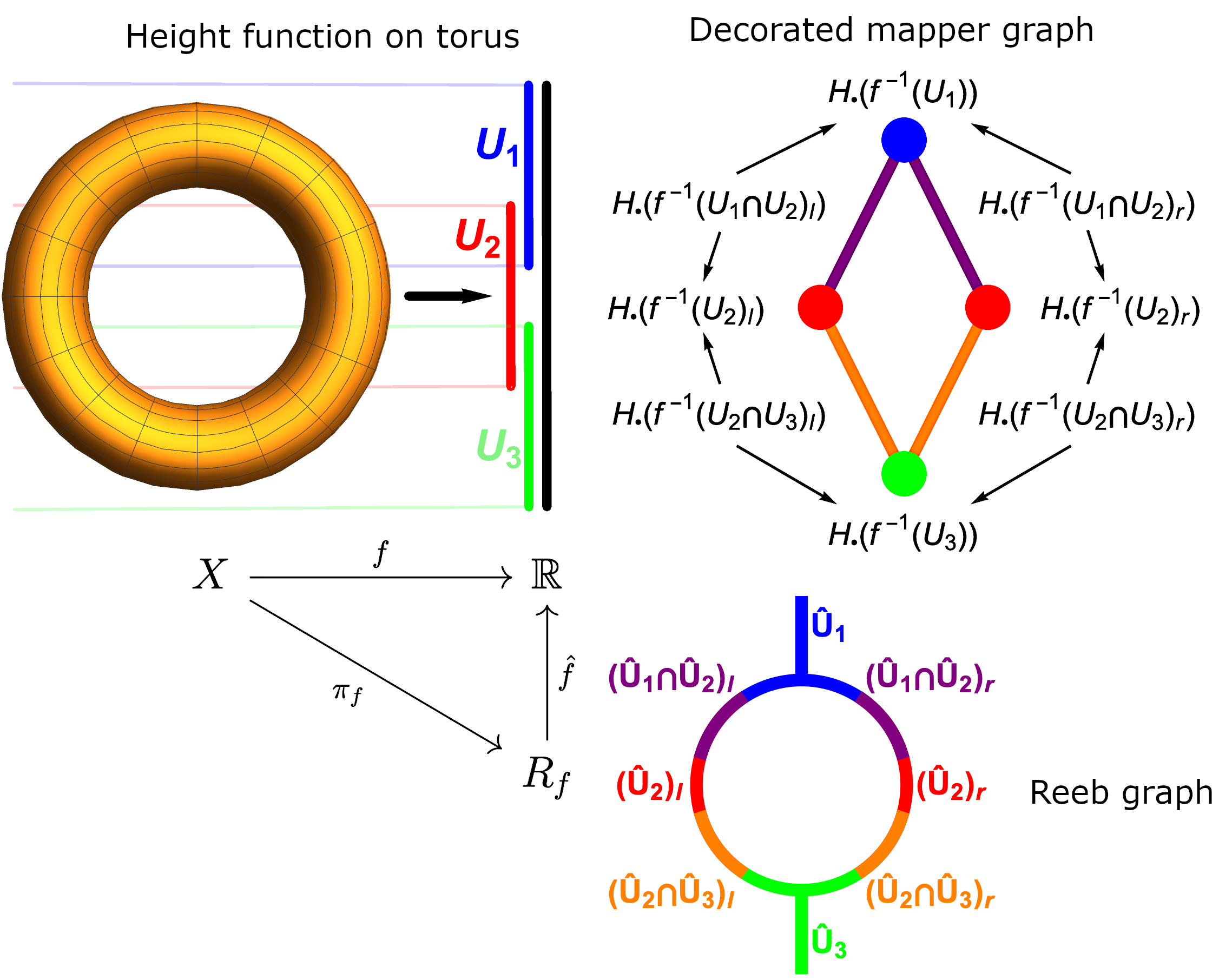
Figure 1: Pulling back the cover $\mathcal{U}$ of $f(X)$ along the induced map $\hat{f}$ on the Reeb graph and refining it into components yields a cover $\hat{\mathcal{U}}$ of $R_{f}$. The decorated mapper graph is the nerve complex of this cover decorated by the homology $H_{\bullet}\big{(}\pi_{f}^{\minus 1}(-)\big{)}$ of the preimages of intersections in $\hat{\mathcal{U}}$ under the quotient map $\pi_{f}$. Since $f=\hat{f}\circ\pi_{f}$, this is analogous to using components of preimages under $f$.

A decorated mapper graph collects the homology (possibly inferred from a point sample) in all degrees $H_{\bullet}(-)\coloneqq\bigoplus_{n\geq 0}H_{n}(-)$ of the components of $f^{\minus 1}(U_{i})$ and $f^{\minus 1}(U_{i}\cap U_{j})$ on the corresponding vertices and edges of the mapper graph; see Figure 1. It can be viewed as a discrete approximation of the Leray cosheaf over the Reeb graph. In this abstract we show that the cellular Leray cosheaf w.r.t. a cover converges to the actual Leray cosheaf for any finite 1D cover $\mathcal{U}$ as the resolution of the cover goes to zero.

2 Leray Cosheaves

The Leray (pre)cosheaf [4, 5, 15] parameterizes the homology of a space $X$ when viewed along a continuous map $f\colon X\rightarrow Y$. It does this by recording for each pair of open subsets $V\subseteq W\subseteq Y$ their homology and the induced map $H_{\bullet}\big{(}f^{\minus 1}(V)\big{)}\xrightarrow{H_{\bullet}(f^{\minus 1}(V)\subseteq f^{\minus 1}(W))}H_{\bullet}\big{(}f^{\minus 1}(W)\big{)}$. We further assume that $X$ is compact and $H_{\bullet}\big{(}f^{\minus 1}(V)\big{)}$ is finite-dimensional for every $V\subseteq Y$.

Definition 2.1 (Leray (pre)cosheaf).

We define the graded Leray (pre)cosheaf $\mathcal{L}^{f}$ of a continuous map $f\colon X\rightarrow Y$ by the following assignments: For all $V\subseteq W\subseteq Y$ open

$$\mathcal{L}^{f}(V)=\bigoplus_{n\in\mathbb{N}_{0}}\mathcal{L}^{f}_{n}(V) \coloneqq\bigoplus_{n\in\mathbb{N}_{0}}H_{n}\big{(}f^{\minus 1}(V)\big{)}$$

$$\mathcal{L}^{f}(V\subseteq W)=\bigoplus_{n\in\mathbb{N}_{0}}\mathcal{L}^{f}_{n}(V\subseteq W) \coloneqq\bigoplus_{n\in\mathbb{N}_{0}}H_{n}\big{(}f^{\minus 1}(V)\subseteq f^{\minus 1}(W)\big{)}\hskip 2.0pt.$$

In practice, we can not access the whole Leray cosheaf. We can only get a cellular version [4, 4.1.6] given by its values on a finite cover of $f(X)$. An open cover $\mathcal{U}=(U_{i})_{i\in I}$ of $f(X)$ defines a simplicial complex $\mathcal{N}_{\mathcal{U}}\coloneqq\{\sigma=(i_{0},\ldots,i_{k})\text{}|\text{ }\mathbf{U}_{\sigma}\coloneqq U_{i_{0}}\cap\ldots\cap U_{i_{k}}\neq\emptyset\}$, called the nerve complex of $\mathcal{U}$. We call $\mathcal{U}$ a finite 1D cover if it is finite and has a one-dimensional nerve complex and denote by $\leq$ the face-relation of $\mathcal{N}_{\mathcal{U}}$, i.e. $\sigma\leq\tau\iff\sigma\text{ is a face of }\tau$ .

Definition 2.2 (Cellular Leray cosheaf).

We define the cellular Leray cosheaf $D_{\mathcal{U}}\mathcal{L}^{f}$ w.r.t. a cover $\mathcal{U}$ as the cosheaf on $\mathcal{N}_{\mathcal{U}}$ given by the following assignments: For all $\sigma\leq\tau\in\mathcal{N}_{\mathcal{U}}$

$$D_{\mathcal{U}}\mathcal{L}^{f}(\sigma) \coloneqq\mathcal{L}^{f}(U_{\sigma})$$

$$D_{\mathcal{U}}\mathcal{L}^{f}(\sigma\leq\tau) \coloneqq\mathcal{L}^{f}(U_{\tau}\subseteq U_{\sigma})\hskip 2.0pt.$$

If $\pi_{f}\colon X\rightarrow R_{f}$ is the quotient map from $X$ to the Reeb graph and $\hat{\mathcal{U}}$ a cover of $R_{f}$, then we define a decorated mapper graph as $D_{\hat{\mathcal{U}}}\mathcal{L}^{\pi_{f}}$; see Figure 1.

3 Convergence

It is obvious that this process of discretization can lose information. This raises the question: How well is $\mathcal{L}^{f}$ represented by $D_{\mathcal{U}}\mathcal{L}^{f}$? To compare $\mathcal{L}^{f}$ and $D_{\mathcal{U}}\mathcal{L}^{f}$, we define a process of transforming $D_{\mathcal{U}}\mathcal{L}^{f}$ into a (pre)cosheaf on $Y$. We want to approximate the value of $\mathcal{L}^{f}$ on any open set $V\subseteq Y$ given only the information in $D_{\mathcal{U}}\mathcal{L}^{f}$. To this end, we define the subcomplex $K_{V}\coloneqq\{\sigma\in\mathcal{N}_{\mathcal{U}}\text{ }|\text{ }U_{\sigma}\cap V\neq\emptyset\}\leq\mathcal{N}_{\mathcal{U}}$, which can be viewed as a simplicial approximation of $V\subseteq\underset{\sigma\in K_{V}}{\bigcup}U_{\sigma}$; see Figure 2. Moreover, if $V\subseteq W$, we obtain an inclusion $\iota\colon K_{V}\xhookrightarrow{}K_{W}$.

Definition 3.1 (Continuous extension).

Let $\mathcal{U}$ be a finite 1D cover of $Y$. We define the continuous extension $C_{\mathcal{U}}D_{\mathcal{U}}\mathcal{L}^{f}$ of $D_{\mathcal{U}}\mathcal{L}^{f}$ as a (pre)cosheaf on $Y$ via the following assignments: For all $V\subseteq W\subseteq Y$ open

$$C_{\mathcal{U}}D_{\mathcal{U}}\mathcal{L}^{f}(V) \coloneqq\bigoplus_{n\in\mathbb{N}_{0}}\Big{(}H_{0}\big{(}K_{V};D_{\mathcal{U}}\mathcal{L}^{f}_{n}|_{K_{V}}\big{)}\oplus H_{1}\big{(}K_{V};D_{\mathcal{U}}\mathcal{L}^{f}_{n\minus 1}|_{K_{V}}\big{)}\Big{)}$$

$$C_{\mathcal{U}}D_{\mathcal{U}}\mathcal{L}^{f}(V\subseteq W) \coloneqq\bigoplus_{n\in\mathbb{N}_{0}}\Big{(}H_{0}\big{(}\iota\big{)}_{n}\oplus H_{1}\big{(}\iota\big{)}_{n\minus 1}\Big{)}$$

where $H_{i}\big{(}K_{V};D_{\mathcal{U}}\mathcal{L}^{f}_{n}|_{K_{V}}\big{)}$ is the degree $i$ homology [4, 6.2.2] of the cosheaf $D_{\mathcal{U}}\mathcal{L}^{f}_{n}$ restricted to $K_{V}$ and $H_{i}(\iota)_{n}$ is the map induced on cosheaf homology by $\iota\colon K_{V}\xhookrightarrow{}K_{W}$ cf. [13, A.17].

As shown in [4, 5, 15], if $\mathcal{U}$ is a finite 1D cover of $f(X)$ the continuous extension yields $C_{\mathcal{U}}D_{\mathcal{U}}\mathcal{L}^{f}(V)\cong\underset{n\in\mathbb{N}_{0}}{\bigoplus}H_{n}\Big{(}f^{\minus 1}\big{(}\underset{\sigma\in K_{V}}{\bigcup}U_{\sigma}\big{)}\Big{)}$ approximating $H_{\bullet}\big{(}f^{\minus 1}(V)\big{)}$; see Figure 2.

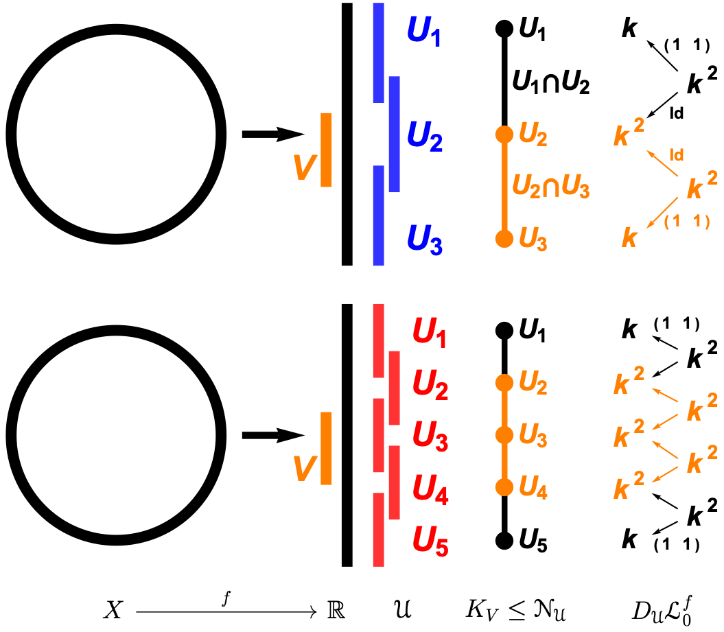
Figure 2: The figure shows $D_{\mathcal{U}}\mathcal{L}^{f}_{0}\cong D_{\mathcal{U}}\mathcal{L}^{f}$ on $\mathcal{N}_{\mathcal{U}}$ w.r.t. two covers with different resolution as well as the restriction $D_{\mathcal{U}}\mathcal{L}^{f}_{0}|_{K_{V}}$ to $K_{V}$ (in orange). Homology is taken with coefficients in a field $k$ and unlabeled arrows represent identity maps. For the coarse cover we get $C_{\mathcal{U}}D_{\mathcal{U}}\mathcal{L}^{f}(V)\cong k\ncong H_{0}\big{(}f^{\minus 1}(V)\big{)}$ but for the finer one we get $C_{\mathcal{U}}D_{\mathcal{U}}\mathcal{L}^{f}(V)\cong k^{2}\cong H_{0}\big{(}f^{\minus 1}(V)\big{)}$.

The following proposition shows that $C_{\mathcal{U}}D_{\mathcal{U}}\mathcal{L}^{f}(V\subseteq W)$ also gives us the correct induced map.

Proposition 3.2.

Let $\mathcal{U}$ be a finite 1D cover of $f(X)$. Then, for all $V\subseteq W\subseteq Y$ open, the following diagram commutes and the horizontal arrows are isomorphisms:

$$\leavevmode\hbox to319.22pt{\vbox to114.94pt{\text{[drawing]}}}\hskip 2.0pt. {H_{0}\big{(}K_{V};D_{\mathcal{U}}\mathcal{L}_{n}^{f}|_{K_{V}}\big{)}\oplus H_{1}\big{(}K_{V};D_{\mathcal{U}}\mathcal{L}_{n\minus 1}^{f}|_{K_{V}}\big{)}} {H_{n}\Big{(}f^{\minus 1}\big{(}\underset{\sigma\in K_{V}}{\bigcup}U_{\sigma}\big{)}\Big{)}} {H_{0}\big{(}K_{W};D_{\mathcal{U}}\mathcal{L}_{n}^{f}|_{K_{W}}\big{)}\oplus H_{1}\big{(}K_{W};D_{\mathcal{U}}\mathcal{L}_{n\minus 1}^{f}|_{K_{W}}\big{)}} {H_{n}\Big{(}f^{\minus 1}\big{(}\underset{\sigma\in K_{W}}{\bigcup}U_{\sigma}\big{)}\Big{)}} \scriptstyle{\cong} \scriptstyle{H_{0}(\iota)\oplus H_{1}(\iota)} \scriptstyle{H_{n}\Big{(}f^{\minus 1}\big{(}\underset{\sigma\in K_{V}}{\bigcup}U_{\sigma}\big{)}\subseteq f^{\minus 1}\big{(}\underset{\sigma\in K_{W}}{\bigcup}U_{\sigma}\big{)}\Big{)}} \scriptstyle{\cong} {H_{0}\big{(}K_{V};D_{\mathcal{U}}\mathcal{L}_{n}^{f}|_{K_{V}}\big{)}\oplus H_{1}\big{(}K_{V};D_{\mathcal{U}}\mathcal{L}_{n\minus 1}^{f}|_{K_{V}}\big{)}} {H_{n}\Big{(}f^{\minus 1}\big{(}\underset{\sigma\in K_{V}}{\bigcup}U_{\sigma}\big{)}\Big{)}} {H_{0}\big{(}K_{W};D_{\mathcal{U}}\mathcal{L}_{n}^{f}|_{K_{W}}\big{)}\oplus H_{1}\big{(}K_{W};D_{\mathcal{U}}\mathcal{L}_{n\minus 1}^{f}|_{K_{W}}\big{)}} {H_{n}\Big{(}f^{\minus 1}\big{(}\underset{\sigma\in K_{W}}{\bigcup}U_{\sigma}\big{)}\Big{)}} \scriptstyle{\cong} \scriptstyle{H_{0}(\iota)\oplus H_{1}(\iota)} \scriptstyle{H_{n}\Big{(}f^{\minus 1}\big{(}\underset{\sigma\in K_{V}}{\bigcup}U_{\sigma}\big{)}\subseteq f^{\minus 1}\big{(}\underset{\sigma\in K_{W}}{\bigcup}U_{\sigma}\big{)}\Big{)}} \scriptstyle{\cong}$$

To talk about convergence, we have to define a distance on (pre)cosheaves. Assume $Y$ is a metric space and that all the involved (pre)cosheaves are constructible [4, 11.0.10]. For every $\epsilon>0$ define $V^{\epsilon}\coloneqq\{y\in Y\text{ }|\text{ }d(y,V)<\epsilon\}$. To a (pre)cosheaf $F$ on $Y$ we now associate $F^{\bullet}\coloneqq\{(F^{\epsilon})_{\epsilon\geq 0}\hskip 2.0pt,\hskip 2.0pt(F_{\epsilon}^{\delta}\colon F^{\epsilon}\rightarrow F^{\delta})_{\epsilon\leq\delta}\}$, a parameterized family of (pre)cosheaves on $Y$, by setting $F^{\epsilon}(V)\coloneqq F(V^{\epsilon})$. This allows us to define the distance of two (pre)cosheaves $F$ and $G$ as the interleaving distance of $F^{\bullet}$ and $G^{\bullet}$, i.e. $d(F,G)\coloneqq d_{I}(F^{\bullet},G^{\bullet})$. Denote by $\text{res}(\mathcal{U})\coloneqq\underset{U\in\mathcal{U}}{\text{sup}}\hskip 2.0pt\underset{x,y\in U}{\text{sup}}d(x,y)$ the resolution of an open cover $\mathcal{U}$. We are now able to show that if the resolution of the cover $\mathcal{U}$ goes to zero, $C_{\mathcal{U}}D_{\mathcal{U}}\mathcal{L}^{f}$ converges to $\mathcal{L}^{f}$.

Theorem 3.3.

If $f\colon X\rightarrow Y$ is continuous and $\mathcal{U}$ is a finite 1D cover of $f(X)$, then

$$d\big{(}C_{\mathcal{U}}D_{\mathcal{U}}\mathcal{L}^{f},\mathcal{L}^{f}\big{)}\leq\text{res}(\mathcal{U})\hskip 2.0pt.$$

If we only consider $\mathcal{L}^{f}_{0}$, the degree-zero part of $\mathcal{L}^{f}$, the construction in Definition 3.1 and Theorem 3.3 specializes to an abelianization of the convergence result in [11].

4 Future Work

Theorem 3.3 guarantees that, if we choose a cover of resolution $\leq\delta$, the cellular Leray cosheaf is a $\delta$-approximation of the continuous one. This result establishes a theoretical justification for working with finite covers. Since we have to deal with maps from finite point sets in practice, in future work we plan to investigate under what conditions we can infer the cellular Leray cosheaf of a map $f\colon X\rightarrow Y$ from a finite sample of $X$; cf. [2].

References

[1]
Ulrich Bauer, Xiaoyin Ge, and Yusu Wang.
Measuring distance between reeb graphs.
In Proceedings of the Thirtieth Annual Symposium on
Computational Geometry, SOCG’14, page 464–473, New York, NY, USA, 2014.
Association for Computing Machinery.
doi:10.1145/2582112.2582169.
[2]
Adam Brown, Omer Bobrowski, Elizabeth Munch, and Bei Wang.
Probabilistic convergence and stability of random mapper graphs.
Journal of Applied and Computational Topology, 5(1):99–140,
2021.
doi:10.1007/s41468-020-00063-x.
[3]
Hamish Carr, Jack Snoeyink, and Ulrike Axen.
Computing contour trees in all dimensions.
Computational Geometry, 24(2):75–94, 2003.
Special Issue on the Fourth CGC Workshop on Computational Geometry.
doi:https://doi.org/10.1016/S0925-7721(02)00093-7.
[4]
Justin Curry.
Sheaves, Cosheaves and Applications.
PhD thesis, University of Pennsylvania, 2014.
arXiv:1303.3255.
[5]
Justin Curry, Robert Ghrist, and Vidit Nanda.
Discrete morse theory for computing cellular sheaf cohomology.
Foundations of Computational Mathematics, 16, 2013.
doi:10.1007/s10208-015-9266-8.
[6]
Vin de Silva, Elizabeth Munch, and Amit Patel.
Categorified reeb graphs.
Discrete & Computational Geometry, 55(4):854–906, 2016.
doi:10.1007/s00454-016-9763-9.
[7]
Barbara Di Fabio and Claudia Landi.
The edit distance for reeb graphs of surfaces.
Discrete & Computational Geometry, 55(2):423–461, 2016.
doi:10.1007/s00454-016-9758-6.
[8]
Herbert Edelsbrunner, John Harer, and Amit K. Patel.
Reeb spaces of piecewise linear mappings.
In Proceedings of the Twenty-Fourth Annual Symposium on
Computational Geometry, SCG ’08, page 242–250, New York, NY, USA, 2008.
Association for Computing Machinery.
doi:10.1145/1377676.1377720.
[9]
Xiaoyin Ge, Issam Safa, Mikhail Belkin, and Yusu Wang.
Data skeletonization via reeb graphs.
Advances in Neural Information Processing Systems, 24, 2011.
[10]
P. Y. Lum, G. Singh, A. Lehman, T. Ishkanov, M. Vejdemo-Johansson,
M. Alagappan, J. Carlsson, and G. Carlsson.
Extracting insights from the shape of complex data using topology.
Scientific Reports, 3(1):1236, 2013.
doi:10.1038/srep01236.
[11]
Elizabeth Munch and Bei Wang.
Convergence between Categorical Representations of Reeb Space and
Mapper.
In 32nd International Symposium on Computational Geometry (SoCG
2016), volume 51 of Leibniz International Proceedings in Informatics
(LIPIcs), pages 53:1–53:16. Schloss Dagstuhl–Leibniz-Zentrum fuer
Informatik, 2016.
doi:10.4230/LIPIcs.SoCG.2016.53.
[12]
Monica Nicolau, Arnold Levine, and Gunnar Carlsson.
Topology based data analysis identifies a subgroup of breast cancers
with a unique mutational profile and excellent survival.
Proceedings of the National Academy of Sciences of the United
States of America, 108:7265–70, 04 2011.
doi:10.1073/pnas.1102826108.
[14]
Gurjeet Singh, Facundo Memoli, and Gunnar Carlsson.
Topological Methods for the Analysis of High Dimensional Data Sets
and 3D Object Recognition.
In Eurographics Symposium on Point-Based Graphics. The
Eurographics Association, 2007.
doi:10.2312/SPBG/SPBG07/091-100.
[15]
Hee Rhang Yoon and Robert Ghrist.
Persistence by parts: Multiscale feature detection via distributed
persistent homology, 2020.
arXiv:2001.01623.