Percolation and conductivity in evolving disordered media

Abstract

Percolation theory and the associated conductance networks have provided deep insights into the flow and transport properties of a vast number of heterogeneous materials and media. In practically all cases, however, the conductance of the networks’ bonds remains constant throughout the entire process. There are, however, many important problems in which the conductance of the bonds evolves over time and does not remain constant. Examples include clogging, dissolution and precipitation, catalytic processes in porous materials, as well as the deformation of a porous medium by applying an external pressure or stress to it that reduces the size of its pores. We introduce two percolation models to study the evolution of the conductivity of such networks. The two models are related to natural and industrial processes involving clogging, precipitation, and dissolution processes in porous media and materials. The effective conductivity of the models is shown to follow known power laws near the percolation threshold, despite radically different behavior both away from and even close to the percolation threshold. The behavior of the networks close to the percolation threshold is described by critical exponents, yielding bounds for traditional percolation exponents. We show that one of the two models belongs to the traditional universality class of percolation conductivity, while the second model yields non-universal scaling exponents.

I Introduction

Percolation theory [1, 2] has provided deep insights into the flow and transport properties of a vast number of heterogeneous materials and media, and has found numerous applications [3] in a variety of contexts. In many cases the heterogeneous materials are represented by conductance networks [4], if a scalar transport process is to be studied; by a network of elastic elements, such as springs [5, 6, 7] or beams [8], if vector transport processes are investigated, or by a network of interconnected pores [9] if one is to examine various fluid flow phenomena in porous materials and media. When representing natural and industrial heterogeneous materials, the conductance of the bonds or pores might be distributed according to some probability distribution function that represents the morphology of the materials [10, 11]. In practically all cases, however, the conductance of the network elements is modeled as constant throughout the percolation process under study.

There are, however, many important problems in which the conductance of the bonds in the networks that represent the morphology of the system of interest evolves over time and, therefore, does not remain constant. One example is non-catalytic gas-solid reactions with solid products, such as sulphation of calcined limestone particles that are highly porous and contain a range of pore sizes,

CaO(s)+SO₂(g)+$$\frac{1}{2} \to$$O₂(g) CaSO₄(s)

Numerous experiments indicate [12, 13] that during the reaction the solid volume increases, and the pores are gradually plugged. Another example is the important problem of catalyst deactivation [14] in which a reactant reacts within the pore space of the catalyst and produces products that not only cover the catalyst’s active sites, but also precipitate on the solid surface of the pores and plug them, leading to deactivation of the catalyst. A third example is the transport of colloidal particles and stable emulsions in flow through a porous medium, during which the particles and emulsions precipitate on the surface of the pores and reduce their flow capacity [15, 16, 17]. The pore space of rock and other natural porous media evolve due to dissolution or precipitation. The fourth example is quartz cementation in sandstone that yields a pore space with a continuous range of various porosity and the corresponding flow and transport properties, such as permeability and electrical conductance. Another example is the evolution of sandstone pore structure in the near-well region by salt precipitation during CO₂ injection for its sequestration [18, 19], as well as during evaporation of brine and the resulting salt precipitation [20, 21, 22]. Pore structure evolution is also observed in systems where the pore sizes of porous materials and, hence, their conductances, are reduced mechanically by, for example, applying an external stress or pressure to the material [23, 24]. In all such cases, and numerous other examples, such as clogging of nanopores by transport of DNA [25], one has an evolving network.

Thus, the purpose of the present paper is to study the transport properties of evolving networks, particularly near their percolation threshold $p_{c}$. The goal of our study is twofold. One is to understand how the transport properties evolve in such networks, and how their evolution depends on the manner by which the conductances decrease. The second goal is to see whether the power-law of percolation theory, according to which the effective conductivity $\sigma_{e}$ follows the universal power law,

$$\sigma_{e}\propto(p-p_{c})^{t}\;,$$ (1)

is also satisfied by the effective conductivity of evolving networks, where $p$ is the fraction of the bonds with a non-zero conductance, and $t$ is the critical exponent whose value is largely universal with $t\simeq 1.3$ in two dimensions.

The rest of this paper is organized as follows. In the next section, we introduce the models that we study and explain how they are employed in our numerical simulations. In Section III, we present the details of the numerical simulations. Section IV presents the results for the power laws that the effective conductivity of the proposed models follow near the percolation threshold, and compares them to the traditional models of random conductance networks. In Sec. V the implications of the results are discussed in detail, while the last section summarizes the results.

II The models

The main motivation for this work is transport in evolving porous media, which typically occurs in complex three-dimensional pore networks. For the sake of more efficient simulations of very large networks, however, we restrict our study to the square lattice, which allows us to make precise comparisons with the existing models.

The simplest network we consider is the traditional square lattice in which we remove bonds by a probability $p$ and where the remaining bonds have unit conductance. For straightforward comparison with models that will be introduced below, we define these networks in the following way [26]: We attribute a random number $p(e)\in[0,1]$ to each bond $e\in E$, where $E$ is the set of bonds in the initial graph, in our case the square lattice. This gives rise to a conductance map $g_{o}\colon E\to\mathbb{R}^{+}$ by letting

$$g_{o}(p,e)=\begin{cases}1&\text{ if }p(e)\leq p\\ 0&\text{ if }p(e)>p\end{cases}$$ (2)

Thus, we attribute unit conductance to all the bonds with a random number smaller than $p$, and zero conductance to the remaining bonds. A conductance map $g$ defines a network, i.e., a weighted graph where the weights represent conductances. To simplify notation we let $g$ represent both the conductance map and the network defined by this map. Networks $g_{o}$ in which the bonds (or sites) are removed (make no contribution to transport) by a certain probability have been widely studied in the classical percolation theory, and are well covered in the literature [1, 2, 3]. They have many interesting properties with known behavior close to the percolation threshold $p_{c}$.

In the model above all bonds have unit conductance. Different transport processes have different relations to, e.g., the cross-sectional area available for transport. For example, the electrical conductance of a cylindrical pipe with a constant cross-sectional area and filled with an electrolyte is proportional to the cross-sectional area, whereas, according to the Hagen-Poiseuille equation, the fluid flow rate through the same cylindrical pipe due to a pressure difference is proportional to the cross-sectional area squared. If we view a bond as a cylindrical pipe of unit length and a variable volume $V_{b}$, then the cross-sectional area will be proportional to the volume, $A_{b}\propto V_{b}$. If a bond weight is assumed to represent its volume or mass, then different transport processes can be represented by raising the weight to a power. In this article, we use mass, instead of volume. For a porous medium, this can be thought of as the mass of the electrolyte or a fluid filling the volume, thereby equating the two through a constant electrolyte of fluid density.

Motivated by evolving porous media, we introduce two types of evolving networks. The first is similar to the networks defined by Eq. (2), but where we have a link weight that is inversely proportional to the probability that the bond is removed. The link weight is set to be equal to the mass, and is expressed as

$$m_{p}(p,e)=\begin{cases}1-p(e)&\text{ if }p(e)\leq p\\ 0&\text{ if }p(e)>p\end{cases}$$ (3)

This type of network is related to clogging of a porous medium, such as a filter or membrane. The model also has a close correspondence with the aforementioned non-catalytic gas-solid reactions and catalyst deactivation when diffusion limits the rate of reaction. As a result, the sizes of the pores are not reduced uniformly. In all such processes, the phenomena begin in a fully connected network, but, over time, the size of the pores gradually decreases due to either a chemical reaction that produces solid products (as in diffusion-limited catalytic or non-catalytic reactions), or by the precipitation of particles on surface of the pores due to the physical interactions between the particles and the pore surface, as in the clogging problems.

The initial network before the onset of the closure process has a mass distribution where $1-p(e)$ is the mass of bond $e$, and the blocking of a bond tends to happen at the least conductive bonds, i.e., the bonds with the smallest mass, thus the smallest $1-p(e)$ values. As discussed above, when the link weight is considered as a mass (or volume), then the weight can be related to various types of transport processes through an exponent $\tau$ as, $g_{p}^{\tau}(p,e)=m_{p}(p,e)^{\tau}$. As described above, $\tau=1$ is related to electrical conductance, while $\tau=2$ is related to fluid flow. For this type of network, the values of the bond conductance have constant value $(1-p(e))^{\tau}$ until removed depending on $p$. The conductance distribution for the network evolves, however, with $p$.

A third type of network is given by the following function:

$$m_{s}(p,e)=\begin{cases}p-p(e)&\text{ if }p(e)\leq p\\ 0&\text{ if }p(e)>p\end{cases}$$ (4)

which is a simple representation of a precipitation/dissolution process, where the precipitation (or, equivalently, the dissolution) is similar throughout the network. This corresponds to the aforementioned catalytic or non-catalytic gas-solid in which diffusion plays no role, and only the kinetics of the reactions are important. For a porous medium, the precipitation reduces the volume of the pores, thereby reducing the original mass $1-p(e)$ by the same mass $1-p$ throughout the network, resulting in a mass of $(1-p(e))-(1-p)=p-p(e)$. Once again, we relate the mass to transport through the exponent $\tau$ as $g_{s}^{\tau}(p,e)=m_{s}(p,e)^{\tau}$. For this type of network, both the bond conductances and their distribution evolve with $p$.

For comparison to the evolving networks that we have introduced, we also consider more traditional networks with a uniform mass distribution between endpoints $a$ and $b$; $U(a,b)$, with $0\leq a<b\leq 1$. Each bond $e$ has two associated probabilities, one for the probability $p(e)\in[0,1]$ of being removed, and one for the mass $m(e)\in[a,b]$ being a random number between $a$ and $b$. The model is then defined by

$$m_{r}(a,b)=\begin{cases}m(e)&\text{ if }p(e)\leq p\\ 0&\text{ if }p(e)>p\end{cases}$$ (5)

Here, we only keep the end-points from the distribution $U(a,b)$ in our notation. This mass model then gives rise to the conductance model $g_{r}^{\tau}(a,b)=m_{r}(a,b)^{\tau}$, so that the mass distribution stays equal to $U(a,b)$ for all $p$ and, as a consequence, the conductance distribution does not evolve with $p$. Later in this paper, we will demonstrate that this type of network is similar to our evolving networks for a restricted range of $p$. As the properties of the $g_{r}^{\tau}(a,b)$ models are known in the literature [27, 28, 29], they will be valuable for comparison with our evolving networks.

Note that the unit conductance in the $g_{0}$ model means that we can equate the conductance map $g_{0}^{\tau}(p,e)$ to a mass model $m_{0}(p,e)$ for all $\tau$. We drop the superscript $\tau$ for the $g_{0}$ models, as they are all equal.

III Computer simulations

All calculations in this study were carried out using the Python programming language. The networks were stored as two lists, one for the vertices, or sites, and one for the edges, or bonds. The reason for using lists instead of, e.g., NumPy arrays (a Python library), is that they are used in several loops, where retrieving values from lists is faster than from arrays. The vertex list stores for each vertex the coordinates, the number of edges connected to the vertex, and the edges identification numbers. The edge list stores the edge identity, the associated random number $p(e)\in[0,1]$, and the identification numbers for the two connected vertices.

Two opposite sides of the networks were considered as the inlet and outlet. For each network, we first determine the percolation threshold $p_{c}$, i.e., the smallest value of $p$ such that the network $g_{o}(p)$ connects the inlet to the outlet. The threshold was computed by a binary search algorithm: The links are ordered according to their value of $p(e)$. We start the binary search by checking if $g_{o}(p)$ is connected when $p$ equals the link value $p(e)$ in the middle of the stack. If it is connected, we remove the upper half of the link stack; if not, we remove the lower half. We then check if $g_{o}(p)$ is connected for $p$ equal to the link value $p(e)$ in the middle of the remaining stack. This process is continued until there is only one link left in the stack, yielding the bridging link at the percolating threshold. In addition, we check during the binary search whether the network is connected by first performing two breadth-first searches [30, 31], one from the inlet and one from the outlet, and then checking the intersection of the resulting two searches; the network is connected if the intersection is nonzero.

To calculate the effective conductance of the networks, we follow the standard approach, namely, applying Kirchhoff’s circuit laws. For each node $i$ we have the equation

$$\sum_{j}g(e)(\phi_{j}-\phi_{i})=0\quad,$$ (6)

where $\phi_{i}$ is the potential at node $i$, and $e$ is the edge $(i,j)$ for the set of nodes $\{j\}$ connected to $i$. The effective conductance is computed by representing the set of equations given by Eq. 6 in matrix form: ${\bf M\Phi}={\bf B}$ [4]. Here, B is the vector representing the boundary conditions. As the boundary conditions, we applied a potential difference between the inlet and outlet. The matrix M represents the discretized Laplacian matrix for the network with the conductance values as weights for the bonds, and is stored in compressed sparse column matrix format using the SciPy library. The matrix $\mathbf{M}$ was inverted using either the conjugate-gradient or the LU-decomposition method, both in the SciPy library, depending on the bandwidth of the matrix. We then obtained the solution vector ${\bf\Phi}={\bf M}^{-1}{\bf B}$, which yields the potentials $\phi_{i}$ in the nodes, from which the total current through the network and, hence, the effective conductance is computed. Dividing the effective conductance by the network size we obtain the effective conductivity $\sigma_{e}$ [1, 3].

For well-connected networks, the approach was efficient and accurate. Close to the percolation threshold, however, where, due to the tortuous and constricted nature of the conducting paths, the current is very unevenly distributed in the network, the matrix inversion is susceptible to numerical errors. To reduce such numerical issues, we construct the Laplacian matrix M of the backbone, where we identify the backbone of the network by a method similar to Tarjan’s strongly connected components algorithm [30, 31], but with a non-recursive implementation in order to avoid stack overflow problems for large network sizes. For each network size, we generated at least 100 realizations and averaged the results.

IV Results and discussion

We now investigate the evolving networks introduced in Section II, both theoretically and numerically. We carried out extensive simulations in order to observe and study the behavior of the effective conductivity of the networks as they evolve.

IV.1 Conductance functions $g_{o}$ and $g_{p}^{\tau}$

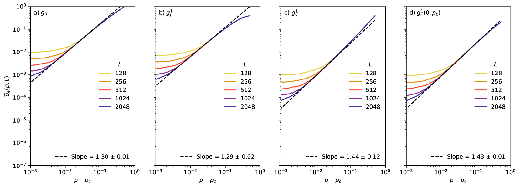
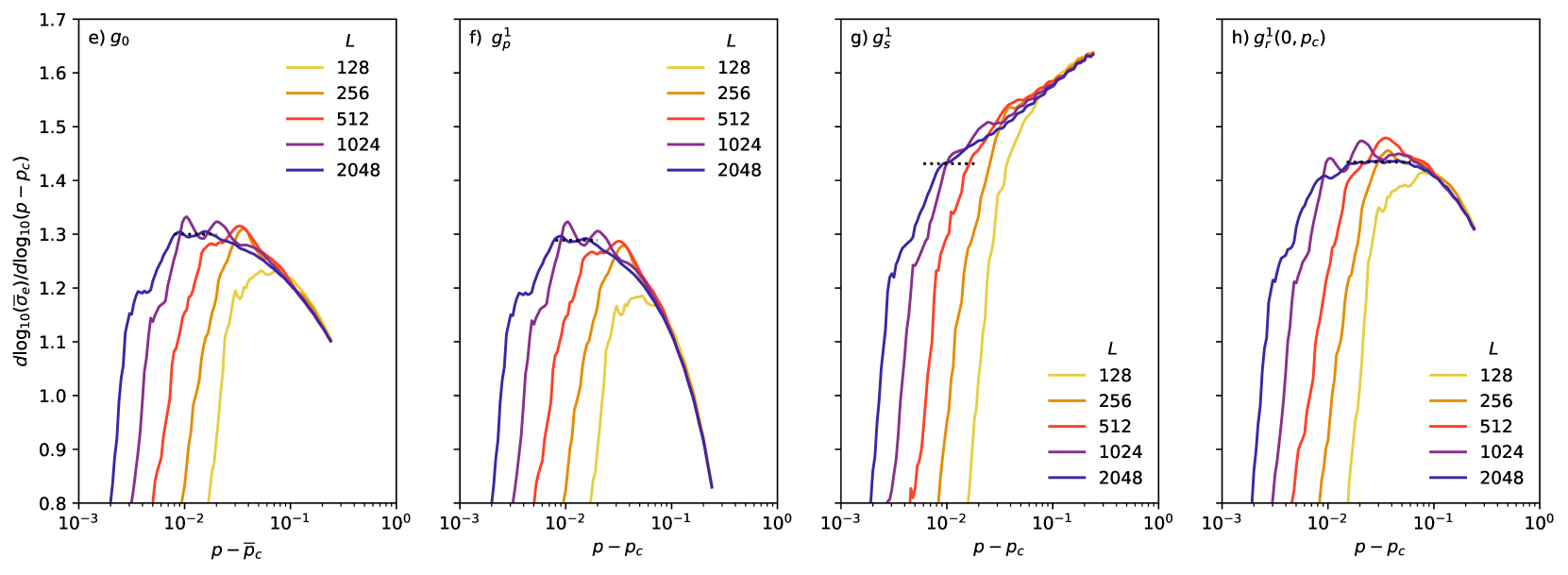
Figure 1: Average effective conductivity $\sigma_{e}$ for 100 realizations for each conductance map $g^{1}$ in (a)-(d), with the corresponding derivatives in (e)-(f). Note that for each of the 100 realizations we have used the same $p(e)$ distribution for the four different conductance maps. The slope is estimated in the range marked by the dotted line in the derivative plots, with the error estimates for the slopes being simply the difference between the minimal and maximal derivative value inside the given range. There is no plateau for the $g_{s}^{1}$ model, and the dashed line range for model $g_{s}^{1}$ in (g) was chosen to obtain a slope similar to the slope for model $g_{r}^{1}$.

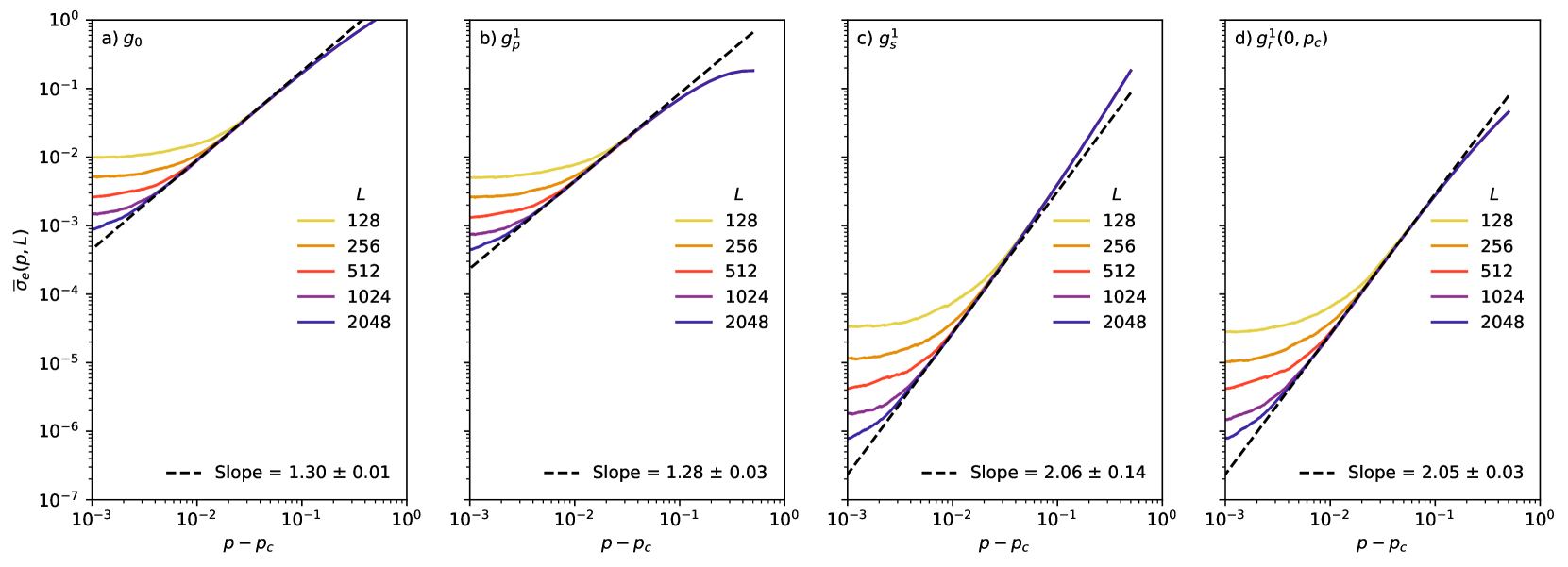
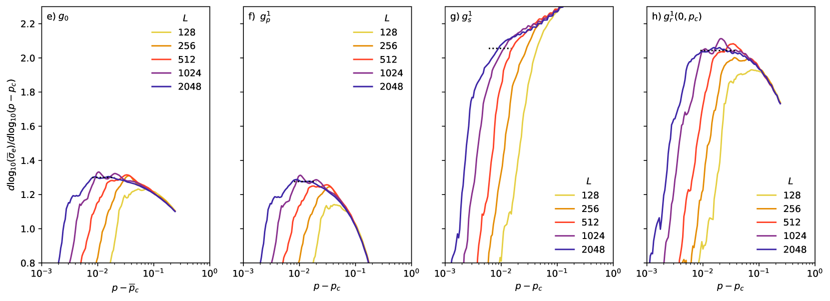
Figure 2: Average effective conductivity $\sigma_{e}$ for 100 realizations for each conductance map $g^{2}$ in (a)-(d), with the corresponding derivatives in (e) and (f). The slope is estimated in the range marked by the dotted line in the derivative plots, with the error estimates for the slopes being simply the difference between the minimal and maximal derivative value inside the given range. Note that the plots for $g_{o}$, in (a) and (e), are equal to the corresponding ones in Figure 1; however, their $y$-scales differ. As with $g_{s}^{1}$, there is no plateau for the $g_{s}^{2}$ model, and the dashed line range for model $g_{s}^{2}$ was chosen to obtain a slope similar to the slope for model $g_{r}^{2}$.

As is well-known, near the percolation threshold $p_{c}$, the effective conductivity of the network $g_{o}$ (i.e., the network resulting from the conductance map $g_{o}$) follows the power law given in Eq. (1) with a critical exponent $t\simeq 1.3$. Figure 1(a) presents the dependence of the average of the effective conductivity $\sigma_{e}^{o}(p,L)$ of 100 realizations of the networks of type $g_{o}(p)$, the standard percolation conductivity model, on both $L$, the linear size of the network, and $(p-p_{c})$. Figure 1(e) shows the numerical derivatives of the curves in Fig. 1 (a). We see that by increasing the size of the network the gradient reaches a plateau with a value close to 1.3 and, thus, $g_{o}$ converge to a power law of type (1) with a slope $t\simeq 1.3$, in agreement with the theoretical expectation.

Next, we investigate the critical exponent for the conductance model $g_{p}^{\tau}$ by identifying an upper and lower bound for the exponent value. The individual bond conductances of $g_{o}$ are always larger or equal to the bond conductances of $g_{p}^{\tau}$ for all $\tau\geq 0$, i.e., $g_{o}\geq g_{p}^{\tau}$ for $\tau\geq 0$. As a consequence of [32, Lemma 11.4], $g_{o}\geq g_{p}^{\tau}$ implies that $\sigma_{e}^{o}(p,L)\geq\sigma_{e}^{p}(p,L)$. If $g_{p}^{\tau}$ follows a universal power law of type (1) with exponent $t_{p}$, then $\sigma_{e}^{p}(p,L)\leq\sigma_{e}^{o}(p,L)$ implies that $t_{p}\geq t=1.3$. Thus, we have identified a lower bound for the exponent $t_{p}$.

We now derive an upper bound for $t_{p}$. For all $p>0$, the smallest bond conductance value in $g_{p}^{\tau}$ is $(1-p)^{\tau}$. If we let $pg_{o}$ denote the network with all bond conductances equal to $p$, then $g_{p}^{\tau}(p,L)>(1-p)^{\tau}g_{o}(p,L)$ for all $p_{c}\leq p<1$. For each $\tau$, since $\sigma_{e}^{p}(1,L)>0$, there exists an $\epsilon>0$ such that $g_{p}^{\tau}(p,L)>\epsilon g_{o}(p,L)$ for all $p_{c}\leq p\leq 1$. The effective conductivity of $\epsilon g_{o}$ is $\epsilon\sigma_{e}^{o}$, where $\sigma_{e}^{o}$ is the effective conductivity of $g_{o}$. As the effective conductivity of $\epsilon g_{o}$ and $g_{o}$ are equal up to a scaling with $\epsilon$, then $\epsilon g_{o}$ has the same power law exponent in Eq. (1) as $g_{o}$, namely, $t\simeq 1.3$. Using the same argument that was utilized for the lower bound, $\sigma_{e}^{p}(p,L)\geq\epsilon\sigma_{e}^{o}(p,L)$ implies that $t_{p}\leq t=1.3$. Since we then have the same lower and upper bound for $t_{p}$, namely, $t\leq t_{p}\leq t$, we have $t_{p}=t\simeq 1.3$. Thus, networks of type $g_{p}^{\tau}$ follow the traditional critical behavior when $p\to p_{c}$.

Next, we consider an alternative method for estimating $t_{p}$. As $p\to p_{c}$, the mass distribution of $g_{p}^{\tau}$ will converge towards the distribution $p_{c}-p(e)$, where $p(e)\in U(p_{c},1)$. Thus, the mass distribution of $g_{p}^{\tau}$ converges towards the mass distribution of a network of type $g_{r}^{\tau}(p_{c},1)$, i.e., a $g_{r}^{\tau}$ function with $m(e)\in U(p_{c},1)$. The networks $g_{r}^{\tau}(p_{c},1)$ and $g_{p}^{\tau}$ are therefore expected to have the same properties when $p\to p_{c}$, including similar critical exponent (this will be substantiated further in the discussion on $g_{s}$ below). We have conducted simulations to confirm such a convergence.

We now use $g_{r}^{\tau}(p_{c},1)$ to obtain the power law description for $g_{p}^{\tau}$. The effective conductivity of $g_{r}^{\tau}(p_{c},1)$ is bounded from above by $g_{o}$ and by $p_{c}^{\tau}g_{o}$ from below. Since $p_{c}^{\tau}g_{o}$ has the same critical exponent $t\simeq 1.3$ as $g_{o}$, then, the critical exponent for $g_{r}^{\tau}(p_{c},1)$ is bounded from both above and below by $t\simeq 1.3$ and, thus, the exponent for $g_{r}^{\tau}(p_{c},1)$ is also $t\simeq 1.3$. As $g_{p}^{\tau}$ and $g_{r}^{\tau}(p_{c},1)$ converge when $p\to p_{c}$, they have the same critical exponents, which provides an alternative proof that $t_{p}\simeq 1.3$.

The results for $t_{p}$ were verified by the simulations. Figure 1(b) and (f) present the average effective conductivity $\sigma_{e}^{p}(p,L)$ and its gradients for the model $g_{p}^{1}$. Similarly, we show the average effective conductivity and gradients for $g_{p}^{2}$ in Fig. 2(b) and (f). The inequality $\sigma_{e}^{o}(p,L)\geq\sigma_{e}^{p}(p,L)$ used to obtain the lower bound for $t_{p}$ can be verified by comparing Fig. 1(a) with Fig. 1(b) and Fig. 2(b). The slope of the $\sigma_{e}^{p}(p,L)$ curves, both for $\tau=1$ in Fig. 1(f) and for $\tau=2$ in Fig. 2(f), converge towards a plateau. While the $\sigma_{e}^{o}$ and $\sigma_{e}^{p}$ curves have different heights, the plateaus of their gradients have similar heights. It is seen that the plateau values for $g_{p}^{1}$ and $g_{p}^{2}$ are in good agreement with the theoretical value of $1.3$. Note that the plots of the derivatives for the $g_{o}$ and $g_{p}^{\tau}$ models have clear similarities, both for $\tau=1$ and 2, as we use the same $p(e)$ distribution for the $g_{o}$ and $g_{p}^{\tau}$ networks.

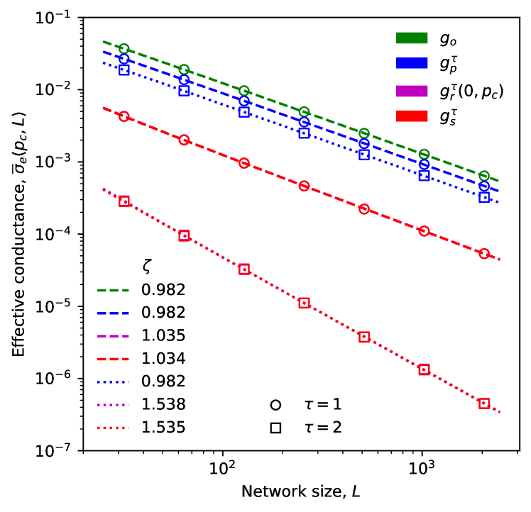
Figure 3: Average effective conductivity $\sigma_{e}$ at the theoretical percolation threshold $p_{c}=0.5$ for more than 5000 realizations of each network size $L$. Note that the curve for $g_{r}^{\tau}$ is covered by the curve for $g_{s}^{\tau}$, as they are basically indistinguishable.

To further investigate the power laws for the various $g$ functions, and in particular $g_{p}$, we consider finite-size scaling at $p_{c}$ [3, 1], namely, $\overline{g}_{e}(p_{c})\propto L^{-t/\nu}$, where $\overline{g}_{e}(p_{c})$ is the average effective conductivity $\sigma_{e}(p_{c})$ at the percolation threshold $p_{c}$ of a large number of network realizations, and $\nu$ is the critical exponent of percolation correlation length with $\nu=4/3$ in 2D. We tested linear regression using both $L^{-\zeta}$ and curves with three free parameters of types suggested in [33]. The curve type yielding the best fit is of the form $L^{-\zeta}(a_{1}-a_{2}/L)$, and is the plot type included in Fig. 3. Note that the other curve types, including $L^{-\zeta}$, yielded similar $\zeta$-exponents.

Figure 3 indicates that finite-size scaling yields an exponent of $\zeta=t/\nu\simeq 0.982$ for the standard percolation conductivity, corresponding to $g_{o}$, close to the expected value of $t/\nu\simeq 0.975$. Note that $m_{p}^{1}>m_{p}^{2}$ since $1-p(e)<1$ (see Eq. 3) and, thus, $g_{o}>g_{p}^{1}>g_{p}^{2}$, as observed in Fig. 3. As discussed above, we expect the same critical exponent for $g_{p}^{\tau}$ as for $g_{o}$. The models associated with $g_{p}^{\tau}$ yield slopes similar to that of $g_{o}$, and the computed $\zeta\approx 0.982$ are consistent with this expectation, yielding $t=\zeta\nu\simeq 1.31\simeq 1.3$.

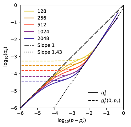
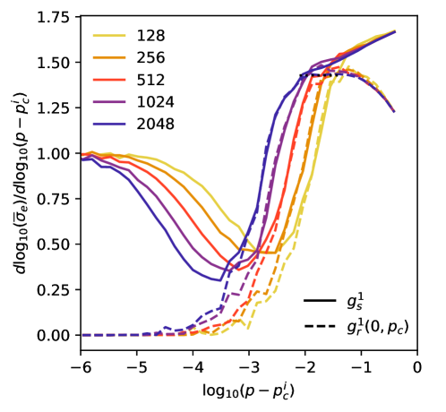
a) b) c)

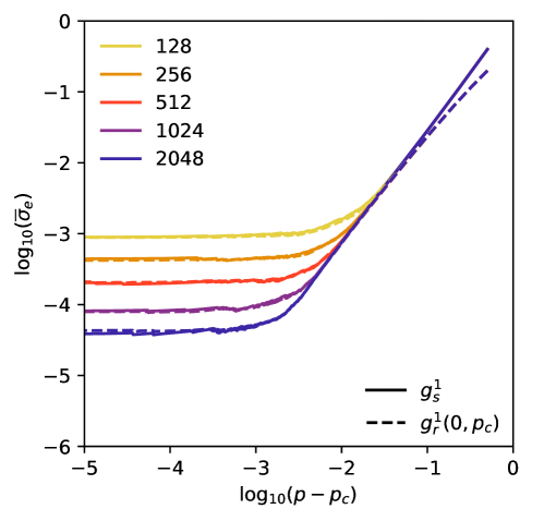
Figure 4: (a) Average effective conductivity $\sigma_{e}$ for the same 100 realizations as used in Fig. 1(c) and (d). They are, however, plotted for the convergence towards their individual thresholds $p-p_{c}^{i}$. (b) Numerical derivatives of the curves in (a), with the dashed line indicating the plateau of the $g_{r}^{1}(p_{c},1)$ curves. The plot in (c) is using the global percolation threshold $p_{c}$, instead of the individual percolation thresholds $p_{c}^{i}$.

IV.2 Conductance function $g_{s}^{\tau}$

A critical difference between models $g_{s}$ and $g_{p}$ is that the conductance distribution of the bonds in $g_{s}$ diverge, which can cause non-universal behavior [27, 29]. Conductance distributions and non-universal behavior will be discussed in the next section. As in the alternative derivation of $t_{p}$, we will use functions of type $g_{r}^{\tau}$ to identify the critical exponents $t_{s}$ for $g_{s}^{\tau}$.

Let $p_{c}^{i}$ be the individual percolation threshold for a given network (one realization of $p(e)$ values). The link with $p(e)=p_{c}^{i}$ is the bridging link, $e_{b}$, which becomes a single connection that keeps the network connected when approaching the individual percolation threshold $p_{c}^{i}$. When $e_{b}$ is removed at $p=p_{c}^{i}$, the remaining network will be disconnected. The conductance of the bridging link will be $(p-p_{c}^{i})^{\tau}\to 0$ when $p\to p_{c}^{i}$, whereas for all other links the conductance $(p-p(e))^{\tau}$ converges to a positive constant. Since the remainder of the network has finite conductance when $p\to p_{c}^{i}$, the resistance of the bridging link will dominate the resistance of the full network in the limit $p\to p_{c}^{i}$. Thus, the effective conductivity scales as $\sigma_{e}\propto(p-p_{c}^{i})^{\tau}L^{2-d}$, when $p\to p_{c}^{i}$ for networks of spatial dimension $d$. In Fig. 4a) we present the effective conductivity of both $g_{s}^{1}$ and $g_{r}^{1}(0,p_{c})$, indicating that the conductivity of $g_{s}^{\tau}$ converges to the slope given by $\tau$, as expected from the derivation above.

If we consider a two-dimensional network $g^{\prime}$ in which all other links than $e_{b}$ in $g_{s}$ are replaced by superconductors, then the network $g^{\prime}$ will have a conductivity $\sigma_{e}^{\prime}\propto(p-p_{c}^{i})^{\tau}$ when $p\to p_{c}^{i}$. Thus, the development of the conductivity is of the power-law type Eq. (1) with critical exponent $\tau$. Since the effective conductivity of $g^{\prime}$ is larger than the conductivity of $g_{s}^{\tau}$, i.e., $\sigma_{e}^{\prime}>\sigma_{e}^{s}$, we see that the critical exponent $t_{s}$ must be bounded below as $t_{s}\geq\tau$. Note that, as the conductivity of $g_{s}^{\tau}$ is always smaller than the conductivity of $g_{o}$ when $\tau>0$, $\sigma_{e}^{o}>\sigma_{e}^{s}$, we also have $t_{s}\geq t=1.3$. Thus, in general, we have, $t_{s}\geq\max(t,\tau)$, giving a lower bound for $t_{s}$.

Consider the situation in which $L\gg\xi$, i.e., one in which $L$ is large compared to the correlation length $\xi$ of percolation. In this limit there are no singly-connected bonds; according to [1] the minimum cut contains approximately $L/\xi$ bonds. As the network is well connected when $L\gg\xi$, we can disregard the effect of the conductance of $e_{b}$ vanishing when $p\to p_{c}^{i}$, as $e_{b}$ is then on one of many connected paths in the infinite percolation cluster. The network will have a mass distribution equivalent to that in $g_{r}^{\tau}(0,p_{c}^{i})$ when $p\to p_{c}^{i}$. To compare our network to $g_{r}^{\tau}(0,p_{c})$, we need $p\simeq p_{c}$ for the distribution of bond conductances in $g_{s}^{\tau}$ to be similar to that in $g_{r}^{\tau}(0,p_{c})$. This requirement does not, however, scale with $L$, so that we can expect the two conductance distributions $g_{s}^{\tau}$ and $g_{r}^{\tau}(0,p_{c})$ to converge at the same values of $p$, independent of the size $L$. Therefore, for large $L$ we can expect a region of $p$ values where $g_{s}^{\tau}\simeq g_{r}^{\tau}(0,p_{c})$, i.e., where $L\gg\xi$ and $p\simeq p_{c}$.

In Fig. 4 we present the results for both $g_{s}^{1}$ and $g_{r}^{1}(0,p_{c})$. As seen in the figure, $g_{s}^{1}$ and $g_{r}^{1}(0,p_{c})$ differ for both large and small values of $p-p_{c}^{i}$; they are, however, similar for a range of intermediate values that correspond to the region in which $L\gg\xi$ and $p\simeq p_{c}$. We also observe that the two curves diverge when $p\to p_{c}^{i}$: In this case, we have $L\ll\xi$ and, thus, the link $e_{b}$ will become the single bridging link. Since the weight $g_{s}^{\tau}(p,e_{b})\to 0$ when $p\to p_{c}^{i}$, this conductance will begin dominating the overall conductance of the network as described above, and the conductance will vanish by the power law, $\sigma_{e}^{s}\propto(p-p_{c}^{i})^{\tau}$, as $p\to p_{c}^{i}$. This is in contrast to the $g_{r}^{\tau}$ network, for which the bridging link $e_{b}$ has a finite conductance, $g_{r}^{\tau}(p,e_{b})>0$ and, thus, $\sigma_{e}^{r}$ converges to a finite value when $p\to p_{c}^{i}$. The two conductance descriptions $g_{s}^{\tau}$ and $g_{r}^{\tau}$ must, therefore, begin to diverge when $p\to p_{c}^{i}$, and Fig. 4 indicates that they do.

While the conductivities have clearly different trajectories when plotted versus their individual percolation thresholds $p_{c}^{i}$, the difference becomes insignificant when one uses instead the traditional averaging $p-p_{c}$, where $p_{c}$ is the percolation threshold for an infinite network. Let $p_{av}=\left<p_{c}^{i}\right>$ be the average of the percolation thresholds for the individual networks, and let $\Delta=\sqrt{\left<(p_{c}^{i})^{2}\right>-\left<p_{c}^{i}\right>^{2}}$ be the standard deviation of the individual percolation thresholds. The two values are known to scale as $p_{av}-p_{c}\propto L^{-1/\nu}$ and $\Delta\propto L^{-1/\nu}$ [1, p. 73]. The standard deviation of the individual percolation thresholds $\Delta$ is larger than the difference between $p_{av}$ and $p_{c}$; thus, the $\Delta\propto L^{-1/\nu}$ correspondence will be of importance to us. The difference between the $g_{s}^{\tau}$ and $g_{r}^{\tau}(0,p_{c})$ models when $p\to p_{c}^{i}$ is expected to be reflected in the $p-p_{c}$ curves only if $\Delta$ is smaller than the onset of divergence between the $g_{s}$ and $g_{r}$ curves. In Fig. 4(c) we have plotted the results for $p-p_{c}$. There is no evident difference between the curves, indicating that $\Delta$ is larger than the onset of the divergence observed in Fig. 4(a) and (b).

Based on the above derivations, the power laws for $g_{s}$ and $g_{r}$ are expected to be the same, and should be bounded from below by $\max(t,\tau)$. This is corroborated by the results in Fig. 3, where the results for $g_{r}^{\tau}(0,p_{c})$ and $g_{s}^{\tau}$ are almost identical for both values of $\tau$. For $\tau=1$ they indicate $\zeta=t_{s}/\nu\simeq 1.034$, which yields a non-universal scaling exponent of $t_{s}\simeq 1.38\geq t=\max(t,\tau)$. For $\tau=2$ we have $\zeta\simeq 1.535$, yielding $t_{s}\simeq 2.05\geq\tau=\max(t,\tau)$.

The results for $g_{s}^{1}$ are presented in Figs. 1(c) and (g), and those for $g_{s}^{2}$ are shown in Figs. 2 (c) and (g). Since $g_{o}>g_{p}^{\tau}>g_{r}^{\tau}$, we have $\sigma_{e}^{o}>\sigma_{e}^{p}>\sigma_{e}^{r}(0,p_{c})$. It is evident from Fig. 1g) that even the largest network size, $L=2048$, does not produce a plateau for the gradient. We thus plot $g_{r}^{1}(0,p_{c})$ in Figs. 1(d) and (h). The derivative indicates a plateau, however, at a value around $t_{s}\simeq 1.43$. This is higher than, $t_{s}=1.38$, obtained from the finite-size scaling above. For $\tau=2$, as seen in Figs. 1(d) and (h), we obtain a slope of $t_{s}\simeq 2.05$, which is in agreement with the finite-size scaling above. These results will be discussed further in the next section.

V Discussion

In the previous section, we investigated the power laws for the effective conductivity of evolving networks, $g_{p}^{\tau}$ and $g_{s}^{\tau}$, introduced in this paper. We argued that the effective conductivities of these networks follow the same power laws as the networks $g_{r}^{\tau}(p_{c},1)$ and $g_{r}^{\tau}(0,p_{c})$, respectively.

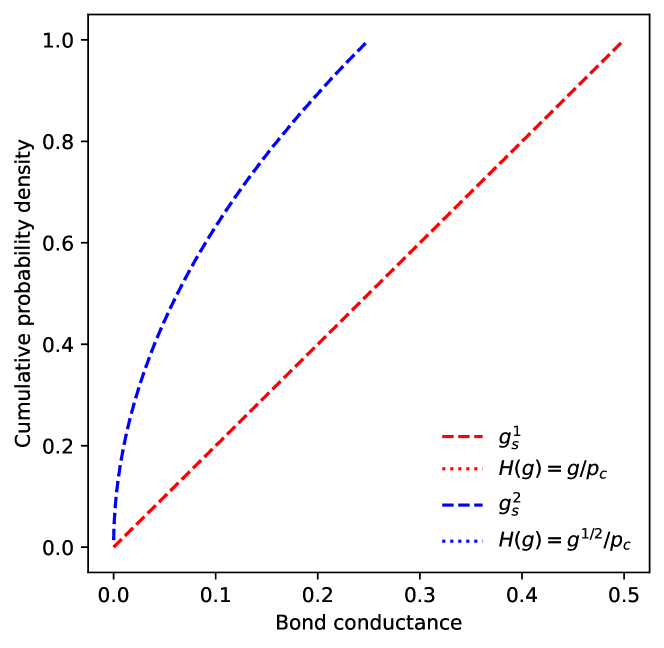
Figure 5: Cumulative conductance distribution for $g_{s}^{\tau}$ for 100 realizations of size $L=512$, together with the functional relationships describing the distribution for $g_{r}^{\tau}(0,p_{c})$. The functional relationships are covered by distributions for $g_{s}^{\tau}$

Non-universality has been observed for networks whose distribution of bond conductances diverges when the conductance values go to zero [27, 29]. For $g_{r}^{\tau}(0,p_{c})$ we have a uniform distribution of bond mass values in the range $[0,p_{c}]$, and the conductance for a bond of mass $m$ is $g=m^{\tau}$. The probability of having a mass smaller than $m$ is $m/p_{c}$. Thus, the probability of having a conductance smaller than $g=m^{\tau}$ becomes $m/p_{c}=g^{1/\tau}/p_{c}$, and the cumulative conductance distribution is given by

$$H(g)=g^{1/\tau}/p_{c}\quad,$$ (7)

for $g\in(0,p_{c}^{\tau})$. In Fig. 5 we present the conductance distribution in $g_{s}^{\tau}$ for the backbone at $p=p_{c}$, together with the distribution function in Eq. (7). We observe an equivalent distribution for $g_{s}^{\tau}$ as $g_{r}^{\tau}(0,p_{c})$.

If we scale the conductances in the range $(0,p_{c}^{\tau}=2^{-\tau})$ to the range $(0,1)$ (with the above notation, we, thus, consider $p_{c}^{-\tau}g_{r}^{\tau}(0,p_{c})$), we have the cumulative probability $H(g)=g^{1/\tau}$, which yields the probability distribution

$$h(g)=\frac{1}{\tau}g^{1/\tau-1}=(1-\alpha)g^{-\alpha}\quad,$$ (8)

where the last term is on the form used in [27], obtained from $\alpha=1-1/\tau$. For $\tau>1$ we have a negative exponent for $g$ in Eq. (8), making $h(g)$ diverge when the conductance $g\to 0$. According to [27], we then have $\sigma_{e}\propto(p-p_{c})^{t_{r}}$, where $t_{r}=t+\alpha/(1-\alpha)=t+\tau-1$, with $t$ being the standard conductivity exponent, with $t\simeq 1.3$ for two-dimensional networks, as mentioned above. Note also that other authors reported different values for $t_{r}$, with $0<t_{r}-t<3/2$ for $\tau=2$ according to [29]. In [28] the non-universal exponent is given as $t_{r}=\max(t,(1-\alpha)^{-1})=\max(t,\tau)$, which is exactly the lower bound we obtained for $g_{s}$ above.

For $\tau=1$ the literature indicates that for the $g_{r}^{\tau}$ model $t_{r}=t\simeq 1.3$. Our derivations above should have yielded $t_{s}=t_{r}=t$, but our numerically computed values for $t_{s}$ are higher than this, with $t_{s}\simeq 1.38$ by finite-size scaling and $t_{s}\simeq 1.43$ through investigating the gradient of the curves $g_{s}(L,p)$. It has been reported that the universality constant for $t_{r}$ is difficult to obtain as logarithmic corrections set in for $\tau=1$ [28]. Our computed values are, however, in excellent agreement with estimates from similar numerical simulations for the $g_{r}^{\tau}$ model [34].

For $\tau=2$, the literature differs on the value of $t_{r}$, with $1.3<t_{r}<2.8$; according to [29], $t_{r}\simeq 2.3$; according to [27], and $t_{r}=2$ according to [28]. Our estimate of $t_{s}\simeq 2.05$ is within the spread of the $t_{r}$ values for the $g_{r}^{\tau}$ model, as indicated by the aforementioned authors.

VI Summary

We introduced two types of evolving networks that are related to natural and industrial processes, such as clogging, precipitation, and dissolution. One model, $g_{p}^{\tau}$, represents clogging processes that tend to block the lowest conducting bonds. The second model, $g_{s}^{\tau}$, represents precipitation processes that reduce the conductance of all bonds similarly. The mass distribution is linked to the conductance by the exponent $\tau$, where $\tau=1$ represents electrical conductance or diffusion, while $\tau=2$ represents fluid flow.

The effective conductivity of the models that we introduced behaves differently from that of the traditional networks $g_{o}$ with constant bond conductance. We showed, however, that the power laws $\sigma_{e}^{p}\propto(p-p_{c})^{t_{p}}$ for $g_{p}^{\tau}$ still belong to the standard universality class with exponent $t_{p}=t\simeq 1.3$.

The effective conductivity of the $g_{s}^{\tau}$ model follows a power law similar to $g_{r}^{\tau}(0,p_{c})$. The effective conductivity of the $g_{r}^{\tau}(0,p_{c})$ model is known in the literature to have non-universal power laws near the percolation threshold, and we have the same non-universality for $g_{s}^{\tau}$. The conductivity of the $g_{s}^{\tau}$ model has, however, a radically different behavior than $g_{r}^{\tau}(0,p_{c})$, when we consider convergence towards individual percolation thresholds, $p\to p_{c}^{i}$. In this limit the $g_{s}^{\tau}$ conductivity scales as $\sigma_{e}^{s}\propto(p-p_{c}^{i})^{\tau}$, which leads to a lower bound $t_{s}\geq\max(t,\tau)$ for the power law, $\sigma_{e}^{s}\propto(p-p_{c})^{t_{s}}$. As the effective conductivity of both $g_{s}$ and $g_{r}(0,p_{c})$ follow the same power laws, this yields the same lower bound for $g_{r}^{\tau}(0,p_{c})$, namely, the lower bound $t_{r}\geq\max(t,\tau)$.

References

- Stauffer and Aharony [2003] D. Stauffer and A. Aharony, Introduction to percolation theory (Taylor & Francis, 2003).
- Saberi [2015] A. A. Saberi, Recent advances in percolation theory and its applications, Physics Reports 578, 1 (2015), publisher: Elsevier.
- Sahimi [2023] M. Sahimi, Applications of percolation theory, 2nd ed. (Springer, New York, 2023).
- Kirkpatrick [1973] S. Kirkpatrick, Percolation and conduction, Reviews of modern physics 45, 574 (1973), publisher: APS.
- Feng and Sen [1984] S. Feng and P. N. Sen, Percolation on elastic networks: new exponent and threshold, Physical review letters 52, 216 (1984), publisher: APS.
- Feng et al. [1984] S. Feng, P. N. Sen, B. I. Halperin, and C. J. Lobb, Percolation on two-dimensional elastic networks with rotationally invariant bond-bending forces, Physical Review B 30, 5386 (1984), publisher: APS.
- Feng and Sahimi [1985] S. Feng and M. Sahimi, Position-space renormalization for elastic percolation networks with bond-bending forces, Physical Review B 31, 1671 (1985), publisher: APS.
- Lewinski [1988] T. Lewinski, Dynamical tests of accuracy of Cosserat models for honeycomb gridworks, (Gesellschaft fuer angewandte Mathematik und Mechanik, Wissenschaftliche Jahrestagung, Stuttgart, Federal Republic of Germany, Apr. 13-17, 1987) Zeitschrift fuer angewandte Mathematik und Mechanik, 68 (1988).
- Sahimi [2011] M. Sahimi, Flow and transport in porous media and fractured rock: from classical methods to modern approaches (John Wiley & Sons, 2011).
- Balberg [1987] I. Balberg, Recent developments in continuum percolation, Philosophical Magazine B 56, 991 (1987), publisher: Taylor & Francis.
- Balberg [2009] I. Balberg, Continuum Percolation, in Encyclopedia of Complexity and Systems Science, edited by R. A. Meyers (Springer New York, New York, NY, 2009) pp. 1443–1475.
- Reyes and Jensen [1987] S. Reyes and K. F. Jensen, Percolation concepts in modelling of gas-solid reactions-III. Application to sulphation of calcined limestone, Chemical engineering science 42, 565 (1987), publisher: Elsevier.
- Shah and Ottino [1987] N. Shah and J. M. Ottino, Transport and reaction in evolving, disordered composites-II. coke deposition in a catalytic pellet, Chemical engineering science 42, 73 (1987), publisher: Elsevier.
- Sahimi and Tsotsis [1985] M. Sahimi and T. T. Tsotsis, A percolation model of catalyst deactivation by site coverage and pore blockage, Journal of Catalysis 96, 552 (1985), publisher: Elsevier.
- Rege and Fogler [1987] S. D. Rege and H. S. Fogler, Network model for straining dominated particle entrapment in porous media, Chemical engineering science 42, 1553 (1987), publisher: Elsevier.
- Sahimi and Imdakm [1991] M. Sahimi and A. O. Imdakm, Hydrodynamics of particulate motion in porous media, Physical Review Letters 66, 1169 (1991), publisher: APS.
- Schwartz et al. [1993] L. M. Schwartz, D. J. Wilkinson, M. Bolsterli, and P. Hammond, Particle filtration in consolidated granular systems, Physical Review B 47, 4953 (1993), publisher: APS.
- Miri and Hellevang [2016] R. Miri and H. Hellevang, Salt precipitation during CO2 storage—A review, International Journal of Greenhouse Gas Control 51, 136 (2016), publisher: Elsevier.
- Jeddizahed and Rostami [2016] J. Jeddizahed and B. Rostami, Experimental investigation of injectivity alteration due to salt precipitation during CO2 sequestration in saline aquifers, Advances in water resources 96, 23 (2016), publisher: Elsevier.
- Rad et al. [2013] M. N. Rad, N. Shokri, and M. Sahimi, Pore-scale dynamics of salt precipitation in drying porous media, Physical Review E 88, 032404 (2013), publisher: APS.
- Rad et al. [2015] M. N. Rad, N. Shokri, A. Keshmiri, and P. J. Withers, Effects of grain and pore size on salt precipitation during evaporation from porous media, Transport in Porous Media 110, 281 (2015), publisher: Springer.
- Dashtian et al. [2018] H. Dashtian, N. Shokri, and M. Sahimi, Pore-network model of evaporation-induced salt precipitation in porous media: The effect of correlations and heterogeneity, Advances in water resources 112, 59 (2018), publisher: Elsevier.
- Richesson and Sahimi [2021a] S. Richesson and M. Sahimi, Flow and transport properties of deforming porous media. II. Electrical conductivity, Transport in Porous Media 138, 611 (2021a), publisher: Springer.
- Richesson and Sahimi [2021b] S. Richesson and M. Sahimi, Flow and transport properties of deforming porous media. I. Permeability, Transport in Porous Media 138, 577 (2021b), publisher: Springer.
- Kubota et al. [2019] T. Kubota, K. Lloyd, N. Sakashita, S. Minato, K. Ishida, and T. Mitsui, Clog and Release, and Reverse Motions of DNA in a Nanopore, Polymers 11, 84 (2019), publisher: MDPI.
- Grimmett [1999] G. Grimmett, Percolation (Springer, 1999).
- Kogut and Straley [1979] P. M. Kogut and J. P. Straley, Distribution-induced non-universality of the percolation conductivity exponents, Journal of Physics C: Solid State Physics 12, 2151 (1979), publisher: IOP Publishing.
- Straley [1982] J. P. Straley, Non-universal threshold behaviour of random resistor networks with anomalous distributions of conductances, Journal of Physics C: Solid State Physics 15, 2343 (1982), publisher: IOP Publishing.
- Feng et al. [1987] S. Feng, B. I. Halperin, and P. N. Sen, Transport properties of continuum systems near the percolation threshold, Physical review B 35, 197 (1987), publisher: APS.
- Tarjan [1972] R. Tarjan, Depth-first search and linear graph algorithms, SIAM journal on computing 1, 146 (1972), publisher: SIAM.
- Sheppard et al. [1999] A. P. Sheppard, M. A. Knackstedt, W. V. Pinczewski, and M. Sahimi, Invasion percolation: new algorithms and universality classes, Journal of Physics A: Mathematical and General 32, L521 (1999), publisher: IOP Publishing.
- Kesten [1982] H. Kesten, Percolation theory for mathematicians, Vol. 194 (Springer, 1982).
- Sahimi and Arbabi [1991] M. Sahimi and S. Arbabi, On correction to scaling for two-and three-dimensional scalar and vector percolation, Journal of statistical physics 62, 453 (1991), publisher: Springer.
- Flukiger et al. [2008] F. Flukiger, F. Plouraboué, and M. Prat, Nonuniversal conductivity exponents in continuum percolating Gaussian fractures, Physical Review E 77, 047101 (2008), publisher: APS.