Analytic calculation of the vison gap in the Kitaev spin liquid

Abstract

Although the ground-state energy of the Kitaev spin liquid can be calculated exactly, the associated vison gap energy has to date only been calculated numerically from finite size diagonalization. Here we show that the phase shift for scattering Majorana fermions off a single bond-flip can be calculated analytically, leading to a closed-form expression for the vison gap energy $\Delta=0.2633J$. Generalizations of our approach can be applied to Kitaev spin liquids on more complex lattices such as the three dimensional hyper-octagonal lattice.

I Introduction

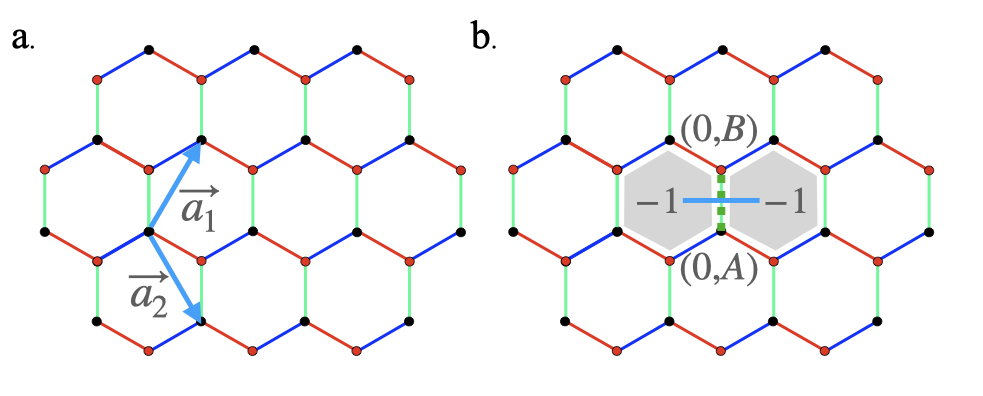
Kitaev spin liquids (KSL) are a class of exactly solvable quantum spin liquid that exhibit spin fractionalization, anyonic excitations and long-range entanglementKitaev (2006); Hermanns et al. (2018); O’Brien et al. (2016); Trebst (2017); Takagi et al. (2019). The fractionalization of spins into Majorana fermions is accompanied by the formation of emergent $\mathbb{Z}_{2}$ gauge fields, giving rise to $\mathbb{Z}_{2}$ vortex excitations or “visons”. These excitations are gapped, and the energy cost associated with creating two visons on adjacent plaquettes is called the vison gap $\Delta_{v}$ (Fig[1]). Proposals for the practical realization of Kitaev spin liquids in quantum materials, including $\alpha$-RuCl₃ Banerjee et al. (2016); Do et al. (2017); Jackeli and Khaliullin (2009); Kasahara et al. (2018); Liu et al. (2020); Takagi et al. (2019); Winter et al. (2017); Wolter et al. (2017); Wulferding et al. (2020); Yamada (2020) and Iridates Chaloupka et al. (2010); Kitagawa et al. (2018); Winter et al. (2017) have renewed interest in the thermodynamics of Kitaev spin liquid Eschmann et al. (2019); Feng et al. (2020); Joy and Rosch (2022); Kato et al. (2017); Li et al. (2020); Nasu et al. (2015); Motome and Nasu (2020); Udagawa and Moessner (2019). The extension of these ideas to Yao-Lee spin liquid Yao and Kivelson (2007); Yao and Lee (2011) and its application to Kondo models, Coleman et al. (2022); Tsvelik and Coleman (2022) motivate the development of an analytical approach to calculate the vison gap $\Delta_{v}$.

The vison gap in KSLs has to date, been determined by numerical diagonalization of finite size systems O’Brien et al. (2016); Kitaev (2006). Here we present a Green’s function approach for the analytical computation of the vison gap $\Delta_{v}$ from the scattering phase shift associated with a a $\mathbb{Z}_{2}$ bond-flip. Our work builds on theoretical developments in the field of Kitaev spin liquids which relate to the interplay between Majorana fermions and visonsKitaev (2006); Baskaran et al. (2007); Knolle et al. (2014); Lahtinen (2011); Lahtinen et al. (2014, 2008, 2012); Théveniaut and Vojta (2017); Kitaev (2006); Joy and Rosch (2022); Kao et al. (2021); Knolle et al. (2014); Lahtinen (2011); Lahtinen et al. (2014, 2008, 2012); Théveniaut and Vojta (2017); Zhang et al. (2019). Using exact calculations, we find the vison gap energy of $\Delta_{v}=0.263313(6)J$ for the Kitaev spin liquid on honeycomb lattice in the gapless phase, extending the accuracy of previous calculations Kitaev (2006); O’Brien et al. (2016). Our calculations reveal the formation of Majorana resonances in the density of states which accompany the formation of two adjacent visons. Our approach can be simply generalized to more complex lattices and are immediately generalizable to Yao-Lee spin liquids.

Figure 1: (a) The Kitaev honeycomb lattice model, where the Ising spin couplings along the x, y and z directions are labelled by blue, green and red bonds respectively, with primitive lattice vectors $\vec{a}_{1}$ and $\vec{a}_{2}$. (b) A bond-reversal at the origin creates a vison pair, costing an energy $\Delta_{v}$. The string connecting the adjacent visons is indicated in light blue.

II Vison Gap in the Kitaev Honeycomb Model

The Kitaev honeycomb lattice model Kitaev (2006) is described by the Hamiltonian

$$H_{K}=\sum_{<ij>}J_{\alpha_{ij}}\sigma^{\alpha_{ij}}_{i}\sigma^{\alpha_{ij}}_{j},$$ (1)

where the Heisenberg spins $\vec{\sigma}_{i}=(\sigma^{x}_{i},\sigma^{y}_{i},\sigma^{z}_{i})$ at site $i$ interact with their nearest neigbors via an Ising coupling between the $\alpha_{ij}=x,y,z$ spin components, along the coresponding bond directions $\langle ij\rangle$, with strength $J_{\alpha_{ij}}$, as shown in Fig[1]. An exact solution of Kitaev Model Kitaev (2006) is found by representing the spins as products of Majorana fermions, $\sigma^{\alpha}_{j}=2c_{j}b^{\alpha}_{j}$ which satisfy canonical anticommutation algebras, $\{c_{i},b^{\alpha}_{j}\}=0$, $\{b^{\alpha}_{i},b^{\beta}_{j}\}=\delta_{ij}\delta^{\alpha,\beta}$, (taking the convention that $c_{j}^{2}=(b_{j}^{\alpha})^{2}=1/2$). The system is projected into the physical subspace by selecting $\mathcal{D}_{j}\equiv-4ic_{j}b^{x}_{j}b^{y}_{j}b^{z}_{j}=1$ at each site, allowing the Hamiltonian (1) to be rewritten as $\mathbb{Z}_{2}$ gauge theory

$$H_{KSL}=2\sum_{<ij>}J_{\alpha_{ij}}\hat{u}_{ij}(ic_{i}c_{j}),$$ (2)

where the gauge fields $\hat{u}_{ij}=2ib^{\alpha_{ij}}_{i}b^{\alpha_{ij}}_{j}=\pm 1$ on bond $ij$ commute with the Hamiltonian, $[\hat{u}_{ij},H_{K}]=0$. The plaquette operators $\mathcal{W}_{p}$

$$\mathcal{W}_{p}=\prod_{<i,j>\in p}u_{ij}\quad(i\in A,j\in B).$$ (3)

formed from the product of gauge fields $\hat{u}_{ij}$ around the hexagonal loop $p$ ( plaquette), are gauge invariant and also commute with the Hamiltonian $[\mathcal{W}_{p},H_{K}]=0$ and constraint operators $[\mathcal{W}_{p},\mathcal{D}_{j}]=0$, giving rise to a set of static constants of motion which take values $\mathcal{W}_{p}=\pm 1$. Each eigenstate is characterized by the configurations of $\{\mathcal{W}_{p}\}$; Lieb’s theorem Lieb (1994) specifies that the ground state configuration is flux-free, i.e. $\mathcal{W}_{p}=1$ for all hexagons $p$. In what follows we will choose the gauge $\hat{u}_{ij}=1$ when $i\in A$ and $j\in B$ sublattice, assigning

$$H_{0}=H_{KSL}[u_{ij}\rightarrow 1].$$ (4)

Rewriting $H_{0}$ in momentum space, we obtain

$$H_{0}=\frac{1}{2}\sum_{{\bf k}\in{\bf BZ}}{\psi}^{\dagger}_{{\bf k}}(\vec{\gamma}_{{\bf k}}\cdot\vec{\tau})\psi_{{\bf k}},$$ (5)

where

$${\psi_{\bf k}}=\frac{1}{\sqrt{N_{c}}}\sum_{j}\left(\begin{array}[]{cc}c_{j,A}\cr c_{j,B}\end{array}\right)e^{-i{\bf{k}}\cdot{\bf R}_{j}}$$ (6)

creates a Majorana in momentum space, where $N_{c}$ is the number of unit cells and ${\bf R}_{j}$ is the location of the unit cell and $\vec{\gamma}_{{\bf k}}=(Re({\gamma_{\bf k}}),-Im(\gamma_{\bf k}))$ is expressed in terms of the form factor

$$\begin{split}\gamma_{\bf k}&=2i(J_{z}+J_{x}e^{ik_{1}}+J_{y}e^{ik_{2}}),\\ {\bf k}&=\frac{k_{1}}{2\pi}{\bf b_{1}}+\frac{k_{2}}{2\pi}{\bf b_{2}},\quad k_{1},k_{2}\in[0,2\pi].\end{split}$$ (7)

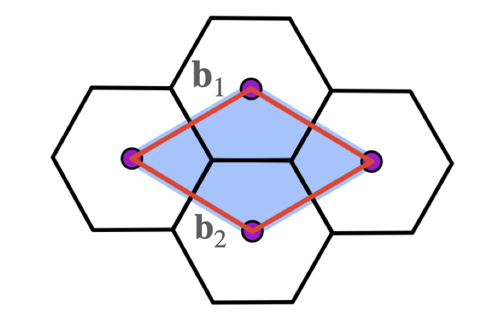
Here we have employed a reciprocal lattice basis ${\bf b_{1},b_{2}}$ to span the momentum ${\bf k}\in{\bf BZ}$, which transforms to rhombus shaped Brillouin zone in the reciprocal lattice (see Fig. 2 ). The Majorana excitation spectrum of the Kitaev spin liquid is given by the eigenvalues of $H_{0}$, $\epsilon_{\bf k}=\pm|\gamma_{\bf k}|$.

Figure 2: Rearranged first Brillouin zone (${\bf BZ}$) constructed in the reciprocal lattice vector basis spanned by ${\bf b_{1}}$ and $\bf{b_{2}}$.

We create two adjacent visons by flipping the gauge field in the unit cell at origin to $\hat{u}_{(0,A)(0,B)}=-1$ as shown in Fig [1], resulting in the following Hamiltonian:

$$H_{KSL+2v}=H_{0}+V,$$ (8)

where

$$\hat{V}=-4J_{z}(ic_{0,A}c_{0,B})$$ (9)

acts as a scattering term for majoranas in the bulk. In this way, the vison gap calculation is formulated as a scattering problem.

For this case, the Hamiltonian is given by

$$\small H_{KSL+2v}=\frac{1}{2}\sum_{{\bf k}\in{\bf BZ}}{\psi}^{\dagger}_{{\bf k}}(\vec{\gamma}_{{\bf k}}\cdot\vec{\tau})\psi_{{\bf k}}+\frac{1}{2}{\bf c}^{T}_{0}(V\tau_{2}){\bf c}_{0},$$ (10)

$${\bf c}_{0}=\left(\begin{array}[]{cc}c_{0,A}\cr c_{0,B}\end{array}\right)=\frac{1}{\sqrt{N_{c}}}\sum_{{\bf k}\in{\bf BZ}}{\psi_{{\bf{k}}}}$$ (11)

creates a Majorana fermion at the origin and $V=4J_{z}$.

We now set up the scattering problem in terms of Green’s functions. The Green’s function of the unscattered majoranas is $G_{0}=G_{0}(i\omega_{n},{\bf k})\delta_{{\bf k},{\bf k^{\prime}}}$, where

$$G_{0}(i\omega_{n},{\bf{k}})=[i\omega_{n}-\vec{\gamma}_{{\bf{k}}}\cdot\vec{\tau}]^{-1}.$$ (12)

In the presence of the bond-flip at the origin, the Green’s function of the scattered majoranas is given by $G=(G_{0}^{-1}-\hat{V})^{-1}$, where $\hat{V}_{{\bf k},{\bf k^{\prime}}}=(V\tau_{2})/N_{c}$ is the scattering matrix. The total free energy of the non-interacting ground-state in the presence of the scattering is given by the standard formula

$$\beta F=-\frac{1}{2}{\hbox{Tr}}[\ln(-G^{-1})]=-\frac{1}{2}{\hbox{Tr}}\ln[-G^{-1}_{0}+\hat{V}],$$ (13)

where ${\rm Tr}$ denotes the full trace over Matsubara frequencies, momenta and sublattice degrees of freedom. The change in free energy is then given by

$$\Delta F=-\frac{1}{2\beta}{\hbox{Tr}}[\ln(1-\hat{V}G_{0})]=\frac{1}{2\beta}\sum_{r=1}^{\infty}\frac{1}{r}{\rm Tr}\bigl{[}(\hat{V}G_{0})^{r}\bigr{]}.$$ (14)

We now carry out the trace over the Matsubara frequencies and momenta, so that

$$\Delta F=\frac{1}{2\beta}\sum_{i\omega_{n}}\sum_{r=1}^{\infty}\frac{1}{r}{\rm tr}\biggl{[}\left(\frac{V\tau_{2}}{N_{c}}\sum_{{\bf{k}}}G_{0}(i\omega_{n},{\bf{k}})\right)^{r}\biggr{]},$$ (15)

where ${\rm tr}\bigl{[}\ \ \bigr{]}$ denotes the residual trace over sublattice degrees of freedom. Now, we can incorporate the summations over momentum by introducing the local Green’s function

$$g(z)=\frac{1}{N_{c}}\sum_{{\bf k}\in\mathbf{BZ}}G_{0}(z,{\bf k}),$$ (16)

so that

$$\Delta F = \frac{1}{2\beta}\sum_{i\omega_{n}}\sum_{r=1}^{\infty}\frac{1}{r}{\rm tr}\left[(V\tau_{2}g(i\omega_{n}))^{r}\right]$$ (17)

$$= -\frac{1}{2\beta}\sum_{i\omega_{n}}{\rm tr}[\ln(1-V\tau_{2}g(i\omega_{n}))],$$ (18)

where we have re-assembled the Taylor series as a logarithm.

Figure 3: Showing real and imaginary parts of (a)$g_{0}(\omega)$ and (b) $g_{2}(\omega)$ as defined in equations (24), (30) and (31).

We shall illustrate our method for the isotropic case $J_{x}=J_{y}=J_{z}=J$, setting $K=2J$ and $V=4J$. In this case, $\gamma_{\bf k}=iK(1+e^{ik_{1}}+e^{ik_{2}})$. If we divide $\gamma_{{\bf{k}}}=i(\gamma_{c}({\bf{k}})+i\gamma_{s}({\bf{k}}))$ into its even and odd components

$$\gamma_{c}({\bf{k}}) = K(1+\cos k_{1}+\cos k_{2}),$$ (19)

$$\gamma_{s}({\bf{k}}) = K(\sin k_{1}+\sin k_{2}),$$ (20)

then $G_{0}(i\omega_{n})$ can be rewritten as

$$g(z)=\frac{1}{N_{c}}\sum_{{\bf k}\in{\bf BZ}}\frac{z-(\gamma_{c}({\bf k})\tau_{2}+\gamma_{s}(\bf{k})\tau_{1})}{z^{2}-|\gamma_{\bf k}|^{2}}.$$ (21)

The odd component $\gamma_{s}(\bf k)$ vanishes under momentum summation so that

$$\begin{split}1-\hat{V}g(z)&=1-\frac{2V}{N_{c}}\sum_{{\bf k}\in\mathbf{BZ}}\frac{z\tau_{2}-\gamma_{c}({\bf k})}{z^{2}-|\gamma_{\bf k}|^{2}}\\ &=1-V(\tau_{2}g_{0}(z)-\mathbb{I}_{2}g_{2}(z))\end{split}$$ (22)

where

$$g_{0}(z) \equiv \frac{1}{N_{c}}\sum_{{\bf k}\in\mathbf{BZ}}\frac{z}{z^{2}-|\gamma_{\bf k}|^{2}},$$ (23)

$$g_{2}(z) \equiv \frac{1}{N_{c}}\sum_{{\bf k}\in\mathbf{BZ}}\frac{\gamma_{c}({\bf k})}{z^{2}-|\gamma_{\bf k}|^{2}}.$$ (24)

Carrying out the trace in the free energy we then obtain

$$\Delta F = -\frac{T}{2}{\hbox{Tr}}\bigl{[}\ln(1-\hat{V}G_{0})\bigr{]}$$

$$= -\frac{T}{2}\sum_{i\omega_{n}}\ln\left[(1+Vg_{2}(i\omega_{n}))^{2}-(Vg_{0}(i\omega_{n}))^{2}\right].$$

The Matsubara summation can then be carried out as an anti-clockwise contour integral around the imaginary axis weighted by Fermi function, $f(z)=[e^{\beta z}+1]^{-1}$. Deforming the contour to run clockwise around the real axis we obtain

$$\Delta F=\int_{-\infty}^{\infty}\frac{d\omega}{2\pi}\left(\frac{1}{2}-f(\omega)\right)\delta_{v}(\omega),$$ (26)

where

$$\delta_{v}(\omega)={\rm Im}\ \ln\biggl{[}(1+2Kg_{2}(z))^{2}-(2Kg_{0}(z))^{2}\biggr{]}_{z=\omega-i\delta}$$ (27)

Figure 4: (a)The scattering phase shift $\delta_{v}(\omega)$ associated with the creation of two adjacent visons, as a function of frequency $\omega$ in units of $K$.(b)Scattering phase shift $\delta_{v}(\omega)$ on an expanded scale, showing inflection point at origin. (c)Resonance in the scattering density of states around $\epsilon_{0}=\pm 0.07K$ in the density of state change $\Delta\rho(\omega)$ due to the bond flip potential, as a function of frequency $\omega$ in units of $K$. This resonance may become sharp in the gapped topological state, signifying vison bound-states.

is identified as the scattering phase shift. Note that $\delta_{v}(\omega)=-\delta_{v}(-\omega)$ is an antisymmetric function of frequency. At zero temperature the vison gap is then

$$\Delta_{v} = -K\int_{-\infty}^{0}\frac{dx}{2\pi}\ {\rm Im}\ln\biggl{[}(1+2g_{2}(z))^{2}-(2g_{0}(z))^{2}\biggr{]}_{z=x-i\delta}$$ (28)

where we have rescaled the frequency in units of $K$, setting $z=\omega/K$. In the reciprocal basis

$$\begin{split}g_{0}(z)=\int_{0}^{2\pi}\frac{dk_{1}}{2\pi}\int_{0}^{2\pi}\frac{dk_{2}}{2\pi}\frac{z}{z^{2}-|\gamma_{\bf k}|^{2}},\\ g_{2}(z)=\int_{0}^{2\pi}\frac{dk_{1}}{2\pi}\int_{0}^{2\pi}\frac{dk_{2}}{2\pi}\frac{\gamma_{c}({\bf k})}{z^{2}-|\gamma_{\bf k}|^{2}},\end{split}$$ (29)

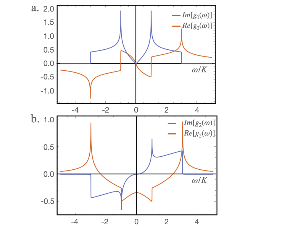
where we have set $K=1$ in $\gamma({\bf{k}})$, i.e $\gamma_{{\bf{k}}}=1+e^{ik_{1}}+e^{ik_{2}}$ and $\gamma_{c}=\cos(k_{1})+\cos(k_{2})$. The interior integral over $k_{2}$ can be carried out as a complex contour integral over $w=e^{ik_{2}}$ around the unit circle, (Appendix A), giving

$$g_{0}(z)=\int_{0}^{2\pi}\frac{dk}{2\pi}\frac{z}{(z^{2}-(3+2c))\sqrt{1-\frac{8(c+1)}{(z^{2}-(3+2c))^{2}}}},$$ (30)

$$g_{2}({z})=\int_{0}^{2\pi}\frac{dk}{2\pi}\frac{2c+1}{({z}^{2}-(3+2c))\sqrt{1-\frac{8(c+1)}{({z}^{2}-(3+2c))^{2}}}},$$ (31)

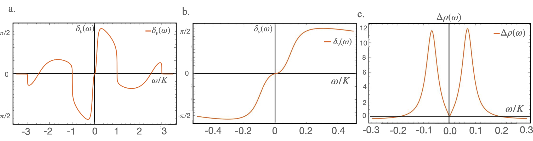
where $c\equiv\cos(k)$. These integrals were evaluated numerically, to obtain the phase shift $\delta_{v}(\omega)$ (Fig[4]). The phase shift was interpolated over over a discrete set of $N$ points and the integral (28) was carried out numerically on the interpolated phase shift. By extrapolating the limit $1/N\rightarrow 0$, we find the vison gap energy to be $\Delta_{v}=0.1311656(3)K=0.263313(6)J$ for the isotropic case $J_{z}=J_{y}=J_{z}=J$.

This analytically-based calculation improves on the earlier result obtained via numerical diagonalization of finite size systems Kitaev (2006) i.e. $\Delta_{v}\approx 0.267J$. Its main virtue however, is that the method can be easily generalized, and we gain insights from the calculated scattering phase shifts.

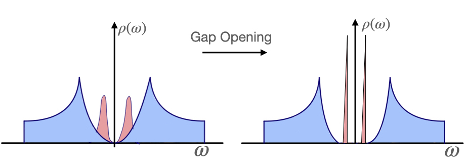
From the calculated phase shift, we can calculate the change in density of states (DOS)

$$\Delta\rho(\omega)=\frac{1}{2\pi}\frac{d\delta_{v}}{d\omega}$$ (32)

(Fig. 4 c.) associated with a Bond flip, which is seen to contain a resonance centered around $\epsilon_{0}\approx\pm 0.07K$. This resonance can be examined in detail by expanding $g_{0}(z)$ and $g_{2}(z)$ for small $z$:

$$\begin{split}g_{0}(\omega)&=\frac{\omega}{\sqrt{3}\pi}\ln\left(\frac{3}{|\omega|}\right)+i\frac{|\omega|}{\sqrt{3}}\\ g_{2}(\omega)&=-\frac{2}{3}-\frac{\omega^{2}}{3\sqrt{3}\pi}\left[\ln\left(\frac{3}{|\omega|}\right)+i\pi{\rm sign}{\ }{\omega}\right]\end{split}$$ (33)

Which can be used to evaluate scattering phase shift $\delta_{v}(\omega)$ (27), and the resonant DOS change $\Delta\rho(\omega)$ (32) analytically. The position of the resonance is determined by the integration over the entire band but its width is determined by the density of states at low energies. Since the DOS vanishes inside the spectral gap, the resonance may become sharp in the topological state. The sharp peak in the gapped state signifies the binding of Majorana fermions to the visons formed by $\mathbb{Z}_{2}$ bond flip at origin.

III Discussion

In this work we have presented an analytical method for determination of the vison gap by treating the flipping of the $\mathbb{Z}_{2}$ gauge field as a scattering potential for the Majorana fermions. In this way, we have been able to analytically extend the numerical treatment by Kitaev for the isotropic model on honeycomb lattice Kitaev (2006) to obtain an analytic result for the vison gap energy $\Delta_{v}$.

Figure 5: Schematic illustration of the resonance in the density of states for the gapless Kitaev spin liquid. The resonance is expected to become sharp when a gap opens in the bulk density of states, forming a fermionic bound-state at the vison pair.

A key part of our approach is the calculation of the Majorana phase shift for scattering off the bond-flipped configuration. One of the interesting observations is that the scattering contains a Majorana bound-state resonance, located at an energy $\epsilon_{0}\approx\pm 0.07K$. Since this bound-state is formed from scattering throughout the entire Brillouin zone, its location is expected to be quite robust. Thus in those cases where the excitation spectrum acquires a gap, eg through time-reversal symmetry breaking Kitaev (2006); Haldane (1988), we expect this resonance to transform into a sharp in-gap excitation.

Figure 6: Hexagonal lattice of Kitaev spin liquid is embedded on a torus by application of periodic boundary condition. An anyons forms within the torus is formed flipping the bonds along a non-contractable loop that encircles the torus.

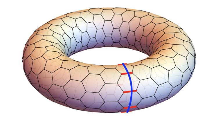
While it is possible to extend our method to analytically calculate the energy associated with anyons by flipping $x-x$ bonds along ${\bf{a_{1}}}$ direction, a much simpler derivation of the anyon energy in the KSL can be made by taking making two copies of the KSL, forming a complex fermion Hamiltonian $H_{c}=H_{KSL}+H_{KSL}$. The line of reverse bonds around the torus can then be absorbed by a unitary transformation that redistributes the odd boundary condition into an effective vector potential that shifts all the momenta ${\bf k}=(k_{1},k_{2})\rightarrow(k_{1}+\frac{\pi}{L},k_{2})$, equivalent to introducing a half magnetic flux with vector potential $A_{x}=\frac{\pi}{L}$. Treating the response to the vector potential in an analogous fashion to a superconductor, the putative the energy cost of an anyon would be

$$\Delta E=\int d^{2}x\frac{\rho_{s}}{4}A_{x}^{2}=\rho_{s}\frac{\pi^{2}}{4},$$ (34)

where $\rho_{s}$ is the superfluid stiffness associated with the ground-state, $A=\pi/L$ is the vector potential and the factor of $4$ derives from halving the energy of the complex fermion system. However, since the complex fermion Hamiltonian $H_{c}$ preserves the global $U(1)$ symmetry, its superfluid stiffness $\rho_{s}$ vanishes so it costs no energy to create anyons in the gapless state. From this line of reasoning, we can see that the ground state of the Kitaev spin liquid has a four-fold degeneracy and is topologically ordered.

Finally, we note that our method also admits various generalizations. For example, it can be extended to anisotropic couplings i.e. $J_{x}\neq J_{y}\neq J_{z}$ as well as to higher dimensions, such as the three-dimensional hyperoctagonal lattice. Moreover, our method can be applied to study the impact of spinor order formation as a consequence of hybridization between conduction electrons and Majorana spinons in the CPT model for a Kondo lattice coupled to a Yao-Lee spin liquid Tsvelik and Coleman (2022); Coleman et al. (2022). This allows us to study the stability of Yao-Lee spin liquid against spinor order formation, the subject of a forthcoming article by the authors.

Appendix A Analytic Calculation of Green’s Function in Honeycomb Lattice

Here we show how to simplify the integrals

$$\begin{split}{g}_{0}(z)=\int_{0}^{2\pi}\frac{dk_{1}}{2\pi}\int_{0}^{2\pi}\frac{dk_{2}}{2\pi}\frac{z}{z^{2}-|\gamma_{\bf k}|^{2}},\\ {g}_{2}(z)=\int_{0}^{2\pi}\frac{dk_{1}}{2\pi}\int_{0}^{2\pi}\frac{dk_{2}}{2\pi}\frac{\gamma_{c}({\bf k})}{z^{2}-|\gamma_{\bf k}|^{2}},\end{split}$$ (35)

where $\gamma_{c}({{\bf{k}}})=1+\cos(k_{1})+\cos(k_{2})$, using a contour integral. We begin by noting that the integrals over $k_{1}$ and $k_{2}$ can be carried out in either order, allowing us to pull the cosines in $\gamma_{c}(k)$ out of the inner integral, so that

$$g_{0}(z) = \int_{0}^{2\pi}\frac{dk_{1}}{2\pi}zI_{0}(z,k_{1}),$$ (36)

$$g_{2}(z) = \int_{0}^{2\pi}\frac{dk_{1}}{2\pi}(1+2\cos k_{1})I_{0}(z,k_{1}),$$ (37)

where

$$I_{0}(z,k)=\int_{0}^{2\pi}\frac{dk_{2}}{2\pi}\frac{1}{z^{2}-|\gamma_{\bf k}|^{2}}.$$ (38)

Writing $s=e^{ik_{1}}$ and $w=e^{ik_{2}}$, we can rewrite $I_{0}$ as a counter-clockwise integral around the unit circle $|w|=1$,

$$I_{0}(z,k)\equiv I_{0}(z,s)=\ointctrclockwise\limits_{|w|=1}\frac{dw}{2\pi iw}\frac{1}{z^{2}-|\gamma(s,w)|^{2}}.$$ (39)

Rewriting the denominator as a quadratic function of $w$,

$$\begin{split}\small z^{2}-|\gamma_{(}s,w)|^{2}&=z^{2}-(1+s+w)(1+\frac{1}{s}+\frac{1}{w})\\ &=-\frac{(1+s)}{sw}(w^{2}+wb+s),\end{split}$$ (40)

where

$$b=\frac{1+3s+s^{2}-sz^{2}}{(1+s)}.$$ (41)

We can thus write the integral in the form

$$I_{0}(z,s)=-\frac{s}{1+s}\ointctrclockwise\frac{dw}{2\pi i}\frac{1}{(w-w_{+})(w-w_{-})}$$ (42)

where

$$w_{\pm}=-\frac{b}{2}\pm\sqrt{\left(\frac{b}{2}\right)^{2}-s}$$ (43)

are the poles of the integrand.

Now since $w_{+}w_{-}=s=e^{ik_{1}}$, it follows that $|w_{+}w_{-}|=1$, so that only one of these poles lies inside the contour. (In general, this may depend on the way we treat the branch cuts inside the square root of (43). However, we don’t actually need to know which pole it is, as this we will fix the sign and the branch-cuts in the final expression by demanding that the asymptotic behavior of $I_{0}\sim 1/z^{2}$ is analytic at large $z$.) Lets assume that the pole closest to the origin is at $w=w_{-}$, then we obtain

$$I_{0}(z,s)=\frac{s}{1+s}\frac{1}{w_{+}-w_{-}}=\frac{s}{1+s}\frac{1}{\sqrt{b^{2}-4s}}.$$ (44)

Now expanding the denominator, we have

$$(1+s)\sqrt{b^{2}-4s} = \sqrt{(1+3s+s^{2}-sz^{2})^{2}-4s(1+s)^{2}}$$ (45)

$$= s\sqrt{(3+2\cos k_{1}-z^{2})^{2}-8(\cos k+1)}$$ (46)

$$= s(z^{2}-(3+2\cos k_{1}))\sqrt{1-\frac{8(\cos k+1)}{(z^{2}-(3+2\cos k_{1}))^{2}}},$$ (47)

where we have factorized the final expression, to guarantee that at large $z$, $I_{0}(z,s)\sim 1/z^{2}$ is analytic. Combining the above results, gives us the following expressions for $g_{0}(z)$ and $g_{2}(z)$

$$\begin{split}{g}_{0}({z})=\int_{0}^{2\pi}\frac{dk}{2\pi}\frac{{z}}{({z}^{2}-(3+2c))\sqrt{1-\frac{8(c+1)}{({z}^{2}-(3+2c))^{2}}}}\\ {g}_{2}(z)=\int_{0}^{2\pi}\frac{dk}{2\pi}\frac{2c+1}{({z}^{2}-(3+2c))\sqrt{1-\frac{8(c+1)}{({z}^{2}-(3+2c))^{2}}}}\end{split}$$ (48)

Where $c\equiv\cos(k)$, which are the expressions given in (30) and (31).

References

- Kitaev (2006) A. Kitaev, Annals of Physics 321, 2 (2006).
- Hermanns et al. (2018) M. Hermanns, I. Kimchi, and J. Knolle, Annual Review of Condensed Matter Physics 9, 17 (2018).
- O’Brien et al. (2016) K. O’Brien, M. Hermanns, and S. Trebst, Physical Review B 93, 085101 (2016).
- Trebst (2017) S. Trebst, (2017), 10.48550/ARXIV.1701.07056, publisher: arXiv Version Number: 1.
- Takagi et al. (2019) H. Takagi, T. Takayama, G. Jackeli, G. Khaliullin, and S. E. Nagler, Nature Reviews Physics 1, 264 (2019).
- Banerjee et al. (2016) A. Banerjee, C. A. Bridges, J.-Q. Yan, A. A. Aczel, L. Li, M. B. Stone, G. E. Granroth, M. D. Lumsden, Y. Yiu, J. Knolle, S. Bhattacharjee, D. L. Kovrizhin, R. Moessner, D. A. Tennant, D. G. Mandrus, and S. E. Nagler, Nature Materials 15, 733 (2016).
- Do et al. (2017) S.-H. Do, S.-Y. Park, J. Yoshitake, J. Nasu, Y. Motome, Y. Kwon, D. T. Adroja, D. J. Voneshen, K. Kim, T.-H. Jang, J.-H. Park, K.-Y. Choi, and S. Ji, Nature Physics 13, 1079 (2017).
- Jackeli and Khaliullin (2009) G. Jackeli and G. Khaliullin, Physical Review Letters 102, 017205 (2009).
- Kasahara et al. (2018) Y. Kasahara, T. Ohnishi, Y. Mizukami, O. Tanaka, S. Ma, K. Sugii, N. Kurita, H. Tanaka, J. Nasu, Y. Motome, T. Shibauchi, and Y. Matsuda, Nature 559, 227 (2018).
- Liu et al. (2020) H. Liu, J. Chaloupka, and G. Khaliullin, Physical Review Letters 125, 047201 (2020).
- Winter et al. (2017) S. M. Winter, A. A. Tsirlin, M. Daghofer, J. van den Brink, Y. Singh, P. Gegenwart, and R. Valentí, Journal of Physics: Condensed Matter 29, 493002 (2017).
- Wolter et al. (2017) A. U. B. Wolter, L. T. Corredor, L. Janssen, K. Nenkov, S. Schönecker, S.-H. Do, K.-Y. Choi, R. Albrecht, J. Hunger, T. Doert, M. Vojta, and B. Büchner, Physical Review B 96, 041405 (2017).
- Wulferding et al. (2020) D. Wulferding, Y. Choi, S.-H. Do, C. H. Lee, P. Lemmens, C. Faugeras, Y. Gallais, and K.-Y. Choi, Nature Communications 11, 1603 (2020).
- Yamada (2020) M. G. Yamada, npj Quantum Materials 5, 82 (2020).
- Chaloupka et al. (2010) J. Chaloupka, G. Jackeli, and G. Khaliullin, Physical Review Letters 105, 027204 (2010).
- Kitagawa et al. (2018) K. Kitagawa, T. Takayama, Y. Matsumoto, A. Kato, R. Takano, Y. Kishimoto, S. Bette, R. Dinnebier, G. Jackeli, and H. Takagi, Nature 554, 341 (2018).
- Eschmann et al. (2019) T. Eschmann, P. A. Mishchenko, T. A. Bojesen, Y. Kato, M. Hermanns, Y. Motome, and S. Trebst, Physical Review Research 1, 032011 (2019).
- Feng et al. (2020) K. Feng, N. B. Perkins, and F. J. Burnell, Physical Review B 102, 224402 (2020).
- Joy and Rosch (2022) A. P. Joy and A. Rosch, Physical Review X 12, 041004 (2022).
- Kato et al. (2017) Y. Kato, Y. Kamiya, J. Nasu, and Y. Motome, Physical Review B 96, 174409 (2017).
- Li et al. (2020) H. Li, D.-W. Qu, H.-K. Zhang, Y.-Z. Jia, S.-S. Gong, Y. Qi, and W. Li, Physical Review Research 2, 043015 (2020).
- Nasu et al. (2015) J. Nasu, M. Udagawa, and Y. Motome, Physical Review B 92, 115122 (2015).
- Motome and Nasu (2020) Y. Motome and J. Nasu, Journal of the Physical Society of Japan 89, 012002 (2020).
- Udagawa and Moessner (2019) M. Udagawa and R. Moessner, (2019), 10.48550/ARXIV.1912.01545, publisher: arXiv Version Number: 1.
- Yao and Kivelson (2007) H. Yao and S. A. Kivelson, Physical Review Letters 99, 247203 (2007).
- Yao and Lee (2011) H. Yao and D.-H. Lee, Physical Review Letters 107, 087205 (2011).
- Coleman et al. (2022) P. Coleman, A. Panigrahi, and A. Tsvelik, Physical Review Letters 129, 177601 (2022).
- Tsvelik and Coleman (2022) A. M. Tsvelik and P. Coleman, Physical Review B 106, 125144 (2022).
- Baskaran et al. (2007) G. Baskaran, S. Mandal, and R. Shankar, Physical Review Letters 98, 247201 (2007).
- Knolle et al. (2014) J. Knolle, D. Kovrizhin, J. Chalker, and R. Moessner, Physical Review Letters 112, 207203 (2014).
- Lahtinen (2011) V. Lahtinen, New Journal of Physics 13, 075009 (2011).
- Lahtinen et al. (2014) V. Lahtinen, A. W. W. Ludwig, and S. Trebst, Physical Review B 89, 085121 (2014).
- Lahtinen et al. (2008) V. Lahtinen, G. Kells, A. Carollo, T. Stitt, J. Vala, and J. K. Pachos, Annals of Physics 323, 2286 (2008).
- Lahtinen et al. (2012) V. Lahtinen, A. W. W. Ludwig, J. K. Pachos, and S. Trebst, Physical Review B 86, 075115 (2012).
- Théveniaut and Vojta (2017) H. Théveniaut and M. Vojta, Physical Review B 96, 054401 (2017).
- Kao et al. (2021) W.-H. Kao, J. Knolle, G. B. Halász, R. Moessner, and N. B. Perkins, Physical Review X 11, 011034 (2021).
- Zhang et al. (2019) S.-S. Zhang, Z. Wang, G. B. Halász, and C. D. Batista, Physical Review Letters 123, 057201 (2019).
- Lieb (1994) E. H. Lieb, Physical Review Letters 73, 2158 (1994).
- Haldane (1988) F. D. M. Haldane, Physical Review Letters 61, 2015 (1988).