Friction mediated phase transition in confined active nematics
Abstract
Using a minimal continuum model, we investigate the interplay between circular confinement and substrate friction in active nematics. Upon increasing the friction from low to high, we observe a dynamical phase transition from a circulating flow phase to an anisotropic flow phase in which the flow tends to align perpendicular to the nematic director at the boundary. We demonstrate that both the flow structure and dynamic correlations in the latter phase differ from those of an unconfined, active turbulent system and may be controlled by the prescribed nematic boundary conditions. Our results show that substrate friction and geometric confinement act as valuable control parameters in active nematics.
A remarkable feature of active fluids is their ability to generate macroscopic flows from energy consumption at the micro-scale [1, 2]. In many cases, however, these flows are chaotic, a phenomenon dubbed “active turbulence” due to its qualitative similarities to inertial turbulence [3, 4, 5, 6, 7, 8, 9, 10, 11, 12]. Identifying methods to control the flows generated by active fluids has recently been of particular interest due to potential technical and biomedical applications. Efforts in this direction have included coupling to concentration gradients, patterning activity, manipulating sample geometry, and imposing boundary conditions [13, 14, 15, 16, 17, 18, 19, 20, 21, 22, 23]. Here, we focus on “active nematics,” active fluids composed of elongated constituents that produce macroscopic flows via force dipoles, and study the flow patterns that emerge from the interplay between two important and relevant control mechanisms: circular confinement [24, 25, 26, 27, 28, 29, 16, 18, 30, 31] and substrate friction [32, 33, 34, 35, 36, 37, 38]. While the effects of these control mechanisms on the dynamical behavior of active nematics have been previously studied independently, their interplay has remained unexplored. Energy dissipation through frictional damping introduces a length scale, the hydrodynamic screening length, which sets the scale below which hydrodynamic interactions are important. Further, because nematics are inherently anisotropic, confinement allows the prescription of topologically and geometrically distinct boundary conditions. While it is known that the boundary conditions do not alter the flow state for frictionless systems [28], it is not known whether a paradigm exists in which the boundary conditions can tune the system dynamics.
Here, using a minimal continuum model, we show that when the hydrodynamic screening length is decreased, circularly confined active nematics transition from a circulating flow state to a dynamical anisotropic flow phase that, to our knowledge, has not been previously described. We show that the anisotropic flow phase is distinct from active turbulence, and is characterized by flows and vortices that organize perpendicular to the nematic boundary condition. As a result, the boundary conditions may be used to tune the dynamics and correlation timescales of the system. To investigate the interplay between confinement and hydrodynamic screening, we vary the screening length at a fixed average time scale associated with active stress injection [39]. This differs from previous investigations of the effects of substrate friction on bulk active nematics in which only the time scale associated with viscous forces is fixed, while the time scale associated with frictional damping is increased leading to the suppression of flow [40, 32, 33, 37]. We find that the anisotropic flow transition occurs when the elastic interactions between defects become dominant due to the hydrodynamic screening length dropping below the size of the topological defects. Our results not only shed light on how biological systems, which tend to have larger screening lengths, organize flow and dynamics, but also can be used to engineer controlled flow and dynamics by employing hydrodynamic screening and boundary conditions as control parameters.
The numerical model we use has been previously well documented [41, 42]. We briefly review it here and give specific details in the Supplementary Material [43]. The equations for the active nematic are written in terms of the nematic tensor order parameter , the fluid velocity , and the fluid pressure :
| (1) | |||
| (2) |
Equation (1) describes the time evolution of the nematic tensor order parameter where gives the local degree of order and is the nematic director. is a generalized tensor advection [44], is the usual Landau-de Gennes free energy in which we assume one-constant elasticity [45], and is a rotational viscosity. Equation (2) is the modified Stokes equation describing low Reynolds number flows. Here is the fluid viscosity. The terms proportional to and are additions to the usual Stokes equation and they describe, respectively, friction between the active nematic and substrate and the strength of active forces in the nematic [42]. corresponds to extensile forces while corresponds to contractile forces. The divergence free condition on the velocity models an incompressible fluid. A discussion of the length and time scales associated with the model is given in the Supplementary Material [43].
We non-dimensionalize, discretize, and solve Eqs. (1) and (2) numerically on a circular domain using fixed nematic boundary conditions with the Matlab/C++ finite element package FELICITY [46]. We fix the domain radius to in dimensionless units (see Supplementary Material [43] for details on dimensionless quantities). We also fix the ratio and vary only the hydrodynamic screening length . The tildes denote dimensionless quantities and are omitted in what follows for brevity. This procedure differs from previous explorations of the effect of friction on bulk active nematics in that we do not hold the viscosity constant [40, 32, 33, 36, 37]. As detailed in the Supplementary Material, constraining the ratio fixes the average active time scale associated with viscous and frictional forces and yields a dimensionless Stokes equation in which the active force is relevant across all scales of the hydrodynamic screening length. This allows us to isolate the effect of the screening length without suppressing the flows generated by the active stress [43]. We choose since this leads to the circulation phase in the zero friction limit for our chosen domain size [28]. Much smaller values lead to a quiescent state, while much larger values lead to turbulent behavior.
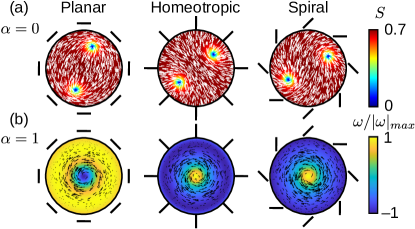
We consider three nematic boundary conditions: planar, homeotropic, and spiral. Figure 1(a) shows the non-active () state for each of these boundary conditions. All three boundary conditions impose an overall topological charge of on the system, so topological defects (points of singular nematic orientation, called disclinations) must form. In the non-active state, the lowest energy configuration consists of two winding number disclinations that lie on opposite ends of the domain. In active nematics, disclinations are motile, and so the configurations we consider show dynamical behavior at lower activities than bulk systems with zero overall topological charge [42].
For the active system (), varying induces a clear transition between two distinct dynamical phases. For large (low friction) the long-time dynamical behavior of the system is characterized by circulating flow. For small (high friction), the circulation ceases and a dynamical anisotropic flow phase reminiscent of active turbulence emerges. Unlike traditional active turbulence, the anisotropic flow is characterized by long, thin vortices that organize near the boundary to lie perpendicular to the nematic director.
The circulation phase observed at large is depicted in Fig. 1(b), where we plot the velocity and vorticity fields for the three boundary conditions at . In all cases, a central vortex is formed and the flow circulates in a clockwise or counter-clockwise direction. For the level of activity we consider, the nematic configuration initially contains two defects circulating each other at early times that eventually merge causing the configuration to develop a central defect with a spiral pattern for all boundary conditions (Fig. S1).
The direction of circulation is a spontaneously broken symmetry for planar and homeotropic anchoring, since these boundary conditions are achiral; however, the spiral boundary conditions break chiral symmetry and always produce counter-clockwise flow. If the boundary conditions were rotated by , the resulting flow would circulate in the opposite direction. Hence, the spiral boundary condition offers a method of controlling the direction of flow, similar to that shown in experiments with bacterial suspensions in a pre-patterned liquid crystal [17] except that it is not necessary to pre-pattern the entire liquid crystal, but only the director at the boundary of the sample.
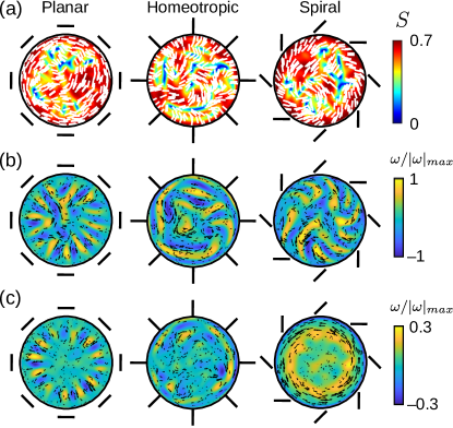
In contrast, the dynamics of the anisotropic flow phase at small depend on the choice of nematic boundary condition. Figures 2(a) and 2(b) show time snapshots of the nematic configuration and velocity and vorticity fields for each boundary condition at . The many long, thin vortices in this phase tend to lie perpendicular to the fixed nematic director at the boundary, and as a result, the flow direction is influenced by the prescribed boundary conditions.
While the anisotropic flow phase is qualitatively reminiscent of traditional active turbulence, we show in Fig. 2(c) that the time-averaged velocity and vorticity fields retain structure when averaged over the length of the simulation. This differs from the zero flow time average obtained in a chaotic, turbulent system, as seen in simulations of unconfined active nematics with periodic boundary conditions (Fig. S2). As shown in Fig. 2(c), for both planar and homeotropic boundary conditions we find persistent organization of vortices near the boundary. The spiral boundary conditions produce time-averaged circulating flow near the boundary instead of the distinct spiral vortex pattern found in the time snapshot of Fig. 2(b). This is because the dynamics of the vortices are relatively static for planar and homeotropic boundary conditions, but circulate for spiral conditions as a result of the promotion of circulating flows (see Supplementary Movies 1–3).
The primary mechanism behind the perpendicular alignment of the flow field to the nematic director at the boundary is the active nematic bend instability [47], which promotes undulations in the nematic director that form parallel to the director. Since controls the size of vortices [32], it also controls the size of the undulations. When is small enough, the undulations become large enough to support the unbinding of disclination pairs that generate flows perpendicular to the director. Thus, the nematic configuration in the anisotropic flow phase is characterized by motile disclinations unbinding near the boundary and then, at a later time, annihilating with immotile disclinations that remain near the boundary (see Supplementary Movies 1–3).
To quantitatively describe the system, we define two parameters related to the velocity of the fluid. The circulation parameter is [29],
| (3) |
where is the azimuthal component of the velocity. All averages are computed over the full simulation time and spatial domain. For coherent circular flows, , while for chaotic, active turbulent flows, . We also measure the average ratio of flow perpendicular to the nematic director boundary condition to that parallel to :
| (4) |
We note that this perpendicular flow measure depends on the boundary condition. For a chaotic, active turbulent state we expect , that is, an equal proportion of perpendicular and parallel flows.
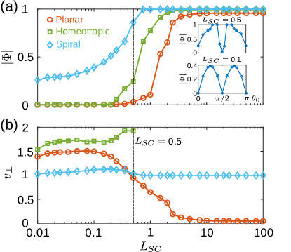
Figure 3 shows and versus for systems with hydrodynamic screening ranging over several orders of magnitude. For planar and homeotropic anchoring, the circulation parameter ranges from at large to at small . The spiral boundary conditions always have nonzero circulation, but decreases as is reduced. We also measured for systems with anchoring angle with respect to the boundary and and , as shown in the inset of Fig. 3(a). We find that in the anisotropic flow phase () the maximal circulation occurs for spiral anchoring, . However, near the phase transition () the circulation is maximal close to planar anchoring, , before dropping to zero exactly at planar anchoring. In this case, the circulating phase is stabilized by the shear flow resulting from the central vortex shown in Fig. 1(b). The nematic tends to align at an angle relative to the flow, the “Leslie angle,” which for our system is close to planar anchoring [48, 43]. Thus, if is close to the Leslie angle, the circulating phase will remain stable for a larger range of . This indicates that the transition itself may be tunable by material parameters that control the flow alignment.
While serves as an order parameter that indicates a transition between dynamical phases, the perpendicular flow parameter quantifies the nature of the anisotropic flow phase at small . Since depends on the director at the boundary, its definition changes for different boundary conditions. For example, for planar boundary conditions we obtain , where is the radial component of the velocity, while for homeotropic boundary conditions we obtain the reciprocal, . For coherent circulating flows, then, goes to zero for planar boundary conditions but diverges for homeotropic boundary conditions. Remarkably, in the anisotropic flow phase is very similar for the planar and homeotropic cases, even though is defined reciprocally. We mark the transition to anisotropic flow in Fig. 3 as occurring at , since below this value, for the three considered boundary conditions. For our choice of model parameters [43], is roughly the radius of the topological defects, suggesting that the hydrodynamic interaction between defects promotes circulation, and that the transition to anisotropic flow occurs when elastic interactions (i.e., Coulomb-like interactions) between defects become dominant.
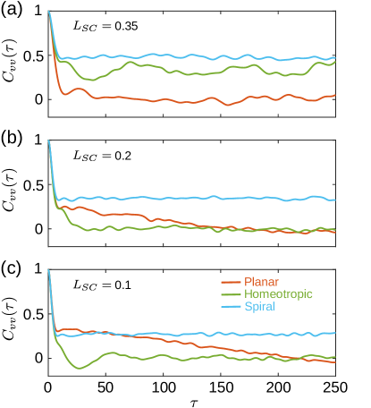
To better understand the dynamics of the anisotropic flow phase, in Fig. 4 we plot the velocity time correlation function
| (5) |
for simulations with , , and . Interestingly, the dynamics differ depending on the boundary condition. Due to the overall circulation, the flows for spiral boundary conditions remain correlated for long times even as is decreased. Near the transition (), however, we find that homeotropic boundary conditions give correlated flows due to the residual circulation present in the system, while planar boundary conditions result in uncorrelated flows. As decreases, systems with homeotropic boundary conditions become uncorrelated, while systems with planar anchoring become more correlated and require longer times to become uncorrelated. Additionally, the velocity correlation functions in the confined system are markedly different from those observed in unconfined systems, which exhibit completely uncorrelated flows at small (Fig. S3).
The differences between the dynamics for planar and homeotropic boundary conditions can be explained by the average structure of the flows shown in Fig. 2(b). For planar anchoring, the vortices on average form an azimuthal periodic structure around the boundary, while for homeotropic anchoring, all periodicity is destroyed as diminishes and the vortices become smaller. These results suggest that both the structure and dynamics of the anisotropic flow phase may be tuned with the nematic boundary condition, which gives insight into how biological systems organize flows and has implications for technological applications of active fluids involving controlled mixing.
Summary— In this work, using the hydrodynamic screening length as a control parameter, we show that circularly confined active nematics transition with decreasing screening length from a circulating flow phase to a previously undescribed anisotropic flow phase characterized by flow organized perpendicularly to the nematic boundary condition. Both dynamical phases feature organized flows distinct from those found in the well-known active turbulent phase. Our work shows that substrate friction and confinement can be used as control mechanisms for the directionality and dynamic correlations of flows via the nematic boundary conditions. While there has been some experimental work in which the substrate is altered such that an effective friction is varied [25, 20], the interplay between confinement and friction has been unexplored experimentally. Following the results of Ref. [20], we propose that the depth of the oil layer may be varied in a circularly confined microtubule based active nematic in order to reproduce our results experimentally. It has additionally been shown both experimentally and numerically that similar transitions occur in three-dimensional active nematics as the system becomes more confined [27, 49, 50]. This indicates that three-dimensional confinement may act as an effective friction on the system and that the complex flows observed may potentially be explained by the simpler two-dimensional model used here.
Future work includes expanding the phase diagram for confined active nematics. In this study we have only varied the screening length , but we expect a rich dynamical phase landscape to emerge as the activity is also varied. This would lead to a better understanding of the interplay between the screening length, the nematic correlation length, and the active length. Additionally, different types of confinement may yield even more modes of control over active systems. We explored the effect of positive curvature, but negative curvature could be induced by a circular inclusion. Experiments in annuli have already shown controlled circulating behavior [27, 16] and immersed microstructures have been shown to pin defects [23]. Due to the increasing degree of experimental and engineered control over boundary geometries and confinement, the understanding of how active fluids interact with their environment is becoming more important and practical.
Acknowledgements.
This work was supported by the U.S. Department of Energy through the Los Alamos National Laboratory. Los Alamos National Laboratory is operated by Triad National Security, LLC, for the National Nuclear Security Administration of the U.S. Department of Energy (Contract No. 89233218CNA000001).References
- Ramaswamy [2010] S. Ramaswamy, The mechanics and statistics of active matter, Annu. Rev. Condens. Matter Phys. 1, 323 (2010).
- Marchetti et al. [2013] M. C. Marchetti, J. F. Joanny, S. Ramaswamy, T. B. Liverpool, J. Prost, M. Rao, and R. A. Simha, Hydrodynamics of soft active matter, Rev. Mod. Phys. 85, 1143 (2013).
- Wensink et al. [2012] H. H. Wensink, J. Dunkel, S. Heidenreich, K. Drescher, R. E. Goldstein, H. Löwen, and J. M. Yeomans, Meso-scale turbulence in living fluids, Proceedings of the National Academy of Sciences 109, 14308 (2012).
- Sanchez et al. [2012] T. Sanchez, D. T. N. Chen, S. J. DeCamp, M. Heymann, and Z. Dogic, Nature 491, 431 (2012).
- Creppy et al. [2015] A. Creppy, O. Praud, X. Druart, P. L. Kohnke, and F. Plouraboué, Turbulence of swarming sperm, Phys. Rev. E 92, 032722 (2015).
- Nishiguchi and Sano [2015] D. Nishiguchi and M. Sano, Mesoscopic turbulence and local order in janus particles self-propelling under an ac electric field, Phys. Rev. E 92, 052309 (2015).
- Yang et al. [2016] T. D. Yang, H. Kim, C. Yoon, S.-K. Baek, and K. J. Lee, Collective pulsatile expansion and swirls in proliferating tumor tissue, New Journal of Physics 18, 103032 (2016).
- Genkin et al. [2017] M. M. Genkin, A. Sokolov, O. D. Lavrentovich, and I. S. Aranson, Topological defects in a living nematic ensnare swimming bacteria, Phys. Rev. X 7, 011029 (2017).
- Doostmohammadi et al. [2017] A. Doostmohammadi, T. N. Shendruk, K. Thijssen, and J. M. Yeomans, Onset of meso-scale turbulence in active nematics, Nat. Commun. 8, 15326 (2017).
- Alert et al. [2020] R. Alert, J.-F. Joanny, and J. Casademunt, Universal scaling of active nematic turbulence, Nature Physics 16, 682 (2020).
- Carenza et al. [2020] L. N. Carenza, L. Biferale, and G. Gonnella, Cascade or not cascade? energy transfer and elastic effects in active nematics, Europhysics Letters 132, 44003 (2020).
- Alert et al. [2022] R. Alert, J. Casademunt, and J.-F. Joanny, Active turbulence, Annual Review of Condensed Matter Physics 13, 143 (2022).
- Guillamat et al. [2016a] P. Guillamat, J. Ignés-Mullol, and F. Sagués, Control of active liquid crystals with a magnetic field, Proceedings of the National Academy of Sciences 113, 5498 (2016a).
- Zhou et al. [2017] S. Zhou, O. Tovkach, D. Golovaty, A. Sokolov, I. S. Aranson, and O. D. Lavrentovich, Dynamic states of swimming bacteria in a nematic liquid crystal cell with homeotropic alignment, New Journal of Physics 19, 055006 (2017).
- Sokolov et al. [2019] A. Sokolov, A. Mozaffari, R. Zhang, J. J. de Pablo, and A. Snezhko, Emergence of radial tree of bend stripes in active nematics, Phys. Rev. X 9, 031014 (2019).
- Hardoüin et al. [2020] J. Hardoüin, J. Laurent, T. Lopez-Leon, J. Ignés-Mullol, and F. Sagués, Active microfluidic transport in two-dimensional handlebodies, Soft Matter 16, 9230 (2020).
- Koizumi et al. [2020] R. Koizumi, T. Turiv, M. M. Genkin, R. J. Lastowski, H. Yu, I. Chaganava, Q.-H. Wei, I. S. Aranson, and O. D. Lavrentovich, Control of microswimmers by spiral nematic vortices: Transition from individual to collective motion and contraction, expansion, and stable circulation of bacterial swirls, Phys. Rev. Res. 2, 033060 (2020).
- Norton et al. [2020] M. M. Norton, P. Grover, M. F. Hagan, and S. Fraden, Optimal control of active nematics, Phys. Rev. Lett. 125, 178005 (2020).
- Reichhardt and Reichhardt [2020] C. Reichhardt and C. J. O. Reichhardt, Directional locking effects for active matter particles coupled to a periodic substrate, Phys. Rev. E 102, 042616 (2020).
- Thijssen et al. [2021] K. Thijssen, D. A. Khaladj, S. A. Aghvami, M. A. Gharbi, S. Fraden, J. M. Yeomans, L. S. Hirst, and T. N. Shendruk, Submersed micropatterned structures control active nematic flow, topology, and concentration, Proceedings of the National Academy of Sciences 118, e2106038118 (2021).
- Vinze et al. [2021] P. M. Vinze, A. Choudhary, and S. Pushpavanam, Motion of an active particle in a linear concentration gradient, Physics of Fluids 33, 032011 (2021).
- Zhang et al. [2021] R. Zhang, S. A. Redford, P. V. Ruijgrok, N. Kumar, A. Mozaffari, S. Zemsky, A. R. Dinner, V. Vitelli, Z. Bryant, M. L. Gardel, and J. J. de Pablo, Spatiotemporal control of liquid crystal structure and dynamics through activity patterning, Nature Materials 20, 875 (2021).
- Figueroa-Morales et al. [2022] N. Figueroa-Morales, M. M. Genkin, A. Sokolov, and I. S. Aranson, Non-symmetric pinning of topological defects in living liquid crystals, Commun. Phys. 5, 301 (2022).
- Wioland et al. [2013] H. Wioland, F. G. Woodhouse, J. Dunkel, J. O. Kessler, and R. E. Goldstein, Confinement stabilizes a bacterial suspension into a spiral vortex, Phys. Rev. Lett. 110, 268102 (2013).
- Guillamat et al. [2016b] P. Guillamat, J. Ignés-Mullol, S. Shankar, M. C. Marchetti, and F. Sagués, Probing the shear viscosity of an active nematic film, Phys. Rev. E 94, 060602 (2016b).
- Theillard et al. [2017] M. Theillard, R. Alonso-Matilla, and D. Saintillan, Geometric control of active collective motion, Soft Matter 13, 363 (2017).
- Wu et al. [2017] K.-T. Wu, J. B. Hishamunda, D. T. N. Chen, S. J. DeCamp, Y.-W. Chang, A. Fernández-Nieves, S. Fraden, and Z. Dogic, Transition from turbulent to coherent flows in confined three-dimensional active fluids, Science 355, eaal1979 (2017).
- Norton et al. [2018] M. M. Norton, A. Baskaran, A. Opathalage, B. Langeslay, S. Fraden, A. Baskaran, and M. F. Hagan, Insensitivity of active nematic liquid crystal dynamics to topological constraints, Phys. Rev. E 97, 012702 (2018).
- Opathalage et al. [2019] A. Opathalage, M. M. Norton, M. P. N. Juniper, B. Langeslay, S. A. Aghvami, S. Fraden, and Z. Dogic, Self-organized dynamics and the transition to turbulence of confined active nematics, Proceedings of the National Academy of Sciences 116, 4788 (2019).
- Mozaffari et al. [2021] A. Mozaffari, R. Zhang, N. Atzin, and J. J. de Pablo, Defect spirograph: Dynamical behavior of defects in spatially patterned active nematics, Phys. Rev. Lett. 126, 227801 (2021).
- Guillamat et al. [2022] P. Guillamat, C. Blanch-Mercader, G. Pernollet, K. Kruse, and A. Roux, Integer topological defects organize stresses driving tissue morphogenesis, Nature Materials 21, 588 (2022).
- Doostmohammadi et al. [2016a] A. Doostmohammadi, M. F. Adamer, S. P. Thampi, and J. M. Yeomans, Stabilization of active matter by flow-vortex lattices and defect ordering, Nat. Commun. 7 (2016a).
- Doostmohammadi et al. [2016b] A. Doostmohammadi, S. P. Thampi, and J. M. Yeomans, Defect-mediated morphologies in growing cell colonies, Phys. Rev. Lett. 117, 048102 (2016b).
- Putzig et al. [2016] E. Putzig, G. S. Redner, A. Baskaran, and A. Baskaran, Instabilities, defects, and defect ordering in an overdamped active nematic, Soft Matter 12, 3854 (2016).
- Srivastava et al. [2016] P. Srivastava, P. Mishra, and M. C. Marchetti, Negative stiffness and modulated states in active nematics, Soft Matter 12, 8214 (2016).
- Doostmohammadi and Yeomans [2019] A. Doostmohammadi and J. M. Yeomans, Coherent motion of dense active matter, Eur. Phys. J. Spec. Top. 227, 2401 (2019).
- Thijssen et al. [2020a] K. Thijssen, L. Metselaar, J. M. Yeomans, and A. Doostmohammadi, Active nematics with anisotropic friction: the decisive role of the flow aligning parameter, Soft Matter 16, 2065 (2020a).
- Thijssen et al. [2020b] K. Thijssen, M. R. Nejad, and J. M. Yeomans, Role of friction in multidefect ordering, Phys. Rev. Lett. 125, 218004 (2020b).
- Giomi et al. [2014] L. Giomi, M. J. Bowick, P. Mishra, R. Sknepnek, and M. Cristina Marchetti, Defect dynamics in active nematics, Philosophical Transactions of the Royal Society A: Mathematical, Physical and Engineering Sciences 372, 20130365 (2014).
- Thampi et al. [2014] S. P. Thampi, R. Golestanian, and J. M. Yeomans, Active nematic materials with substrate friction, Phys. Rev. E 90, 062307 (2014).
- Marenduzzo et al. [2007] D. Marenduzzo, E. Orlandini, M. E. Cates, and J. M. Yeomans, Steady-state hydrodynamic instabilities of active liquid crystals: Hybrid lattice boltzmann simulations, Phys. Rev. E 76, 031921 (2007).
- Doostmohammadi et al. [2018] A. Doostmohammadi, J. Ignés-Mullol, J. M. Yeomans, and F. Sagués, Active nematics, Nat. Commun. 9, 3246 (2018).
- [43] See Supplemental Material for details on the continuum model, numerical method, unconfined active nematic simulations, and supplementary figures and videos.
- Beris and Edwards [1994] A. N. Beris and B. J. Edwards, Thermodynamics of flowing systems (Oxford University Press, 1994).
- de Gennes [1975] P. G. de Gennes, The Physics of Liquid Crystals (Oxford University Press, 1975).
- Walker [2018] S. W. Walker, Felicity: A matlab/c++ toolbox for developing finite element methods and simulation modeling, SIAM J. Sci. Comput. 40, C234 (2018).
- Ramaswamy and Rao [2007] S. Ramaswamy and M. Rao, Active-filament hydrodynamics: instabilities, boundary conditions and rheology, New Journal of Physics 9, 423 (2007).
- Leslie [1992] F. M. Leslie, Continuum theory for nematic liquid crystals, Continuum Mech. Thermodyn. 4, 167 (1992).
- Chandragiri et al. [2020] S. Chandragiri, A. Doostmohammadi, J. M. Yeomans, and S. P. Thampi, Flow states and transitions of an active nematic in a three-dimensional channel, Phys. Rev. Lett. 125, 148002 (2020).
- Varghese et al. [2020] M. Varghese, A. Baskaran, M. F. Hagan, and A. Baskaran, Confinement-induced self-pumping in 3d active fluids, Phys. Rev. Lett. 125, 268003 (2020).