Online On-Demand Multi-Robot Coverage Path Planning

Abstract

We present an online centralized path planning algorithm to cover a large, complex, unknown workspace with multiple homogeneous mobile robots. Our algorithm is horizon-based, synchronous, and on-demand. The recently proposed horizon-based synchronous algorithms compute all the robots’ paths in each horizon, significantly increasing the computation burden in large workspaces with many robots. As a remedy, we propose an algorithm that computes the paths for a subset of robots that have traversed previously computed paths entirely (thus on-demand) and reuses the remaining paths for the other robots. We formally prove that the algorithm guarantees complete coverage of the unknown workspace. Experimental results on several standard benchmark workspaces show that our algorithm scales to hundreds of robots in large complex workspaces and consistently beats a state-of-the-art online centralized multi-robot coverage path planning algorithm in terms of the time needed to achieve complete coverage. For its validation, we perform ROS+Gazebo simulations in five $2$D grid benchmark workspaces with $10$ Quadcopters and $10$ TurtleBots, respectively. Also, to demonstrate its practical feasibility, we conduct one indoor experiment with two real TurtleBot2 robots and one outdoor experiment with three real Quadcopters.

I Introduction

Coverage Path Planning (CPP) deals with finding conflict-free routes for a fleet of robots to make them completely visit the obstacle-free regions of a given workspace to accomplish some designated task. It has numerous applications in indoor environments, e.g., vacuum cleaning [1, 2], industrial inspection [3], etc., as well as in outdoor environments, e.g., road sweeping [4], lawn mowing [5], precision farming [6], [7], surveying [8], [9], search and rescue operations [10], [11], demining a battlefield [12], etc. A CPP algorithm, often called a Coverage Planner (CP), is said to be complete if it guarantees coverage of the entire obstacle-free region. Though a single robot is enough to achieve complete coverage of a small environment (e.g., [13, 14, 15], [16, 17], [18, 19], [20]), multiple robots (e.g., [21, 22, 23], [24, 9], [2, 25, 26, 27]) facilitate complete coverage of a large environment more quickly. However, the design complexity of the CP grows significantly to exploit the benefit of having multiple robots.

For many CPP applications, the workspace’s obstacle map is unknown initially. So, the offline CPs (e.g., [28, 29, 30], [14, 1], [24, 31, 32, 33]) that require the obstacle map beforehand are not applicable here. Instead, we need an online CP (e.g., [34], [35], [36], [37, 38], [39, 40, 25], [41]) that runs through multiple rounds to cover the entire workspace gradually. In each round, the robots explore some unexplored regions using attached sensors, and the CP subsequently finds their subpaths to cover the explored obstacle-free regions not covered so far, a.k.a. goals.

Based on where the CP runs, we can classify it as either centralized or distributed. A centralized CP (e.g., [42, 34, 36], [30], [14, 39, 15], [24, 43], [44]) runs at a server and is responsible for finding all the paths alone. In contrast, a distributed CP (e.g., [45], [46], [47, 48, 49], [50], [51, 52, 53]) runs at every robot as a local instance, and these local instances collaborate among themselves to find individual paths. The distributed CPs are computationally faster as they deal with only the local state spaces. However, they find highly inefficient paths due to the lack of global knowledge about the state space. Despite having high computation time, the centralized CPs can provide a shorter coverage completion time as they can find highly efficient paths by exploiting the global state space. The recently proposed receding horizon-based (e.g., [36, 39]) online multi-robot centralized coverage planner GAMRCPP [44] demonstrates this capability, thereby outperforming the state-of-the-art online multi-robot distributed coverage planner $\mathtt{BoB}$ [50].

A major bottleneck of GAMRCPP is that it generates the paths for all the robots synchronously (i.e., at the same time) in each horizon (like [39]), which prevents it from scaling for hundreds of robots in large workspaces. Furthermore, GAMRCPP decides the horizon length based on the minimum path length and discards the remaining paths for the robots with longer paths. Finding a better goal assignment for those robots in the next horizon is possible, but discarding the already generated paths leads to considerable computational wastage. In this paper, we propose an alternative approach where, like GAMRCPP, the CP decides the horizon length based on the minimum path length but keeps the remaining paths for the robots with longer paths for traversal in the subsequent horizons. Thus, in a horizon, our proposed CP has to synchronously generate the paths for only those robots for which no remaining path is available (called the participant robots), hence on-demand. However, this new on-demand approach brings the additional challenge of computing the new paths under the constraint of the remaining paths for some robots. Our CP tackles this challenge soundly. Though the proposed approach misses the opportunity to find more optimal paths for the non-participant robots in a horizon, the computation load in each horizon decreases significantly, which in turn leads to a faster coverage completion of large workspaces with hundreds of robots, promising scalability.

We formally prove that the proposed CP can achieve complete coverage. To evaluate its performance, we consider eight large $2$D grid-based benchmark workspaces of varying size and obstacle density and two types of robots, TurtleBot [54], which is a ground robot, and Quadcopter, which is an aerial robot, for their coverage. We vary the number of robots from $128$ to $512$ and choose mission time as the comparison metric, which is the time required to attain complete coverage. We compare our proposed CP with GAMRCPP and show that it outperforms GAMRCPP consistently in large workspaces involving hundreds of robots. We further demonstrate the practical feasibility of our algorithm through ROS+Gazebo simulations and real experiments.

II Problem

II-A Preliminaries

Let $\mathbb{R}$ and $\mathbb{N}$ denote the set of real numbers and natural numbers, respectively, and $\mathbb{N}_{0}$ denote the set $\mathbb{N}\cup\{0\}$. Also, for $m\in\mathbb{N}$, we write $[m]$ to denote the set $\{n\in\mathbb{N}\,|\,n\leq m\}$, and $[m]_{0}$ to denote the set $[m]\cup\{0\}$. The size of the countable set $\mathcal{S}$ is denoted by $|\mathcal{S}|\in\mathbb{N}_{0}$. Furthermore, we denote the set $\{0,1\}$ of Boolean values by $\mathbb{B}$.

II-A1 Workspace

We consider an unknown $2$D workspace $W$ represented as a grid of size $X\times Y$, where $X,Y\in\mathbb{N}$. Thus, $W$ is represented as a set of non-overlapping square-shaped grid cells $\{(x,y)\,|\,x\in[X]\wedge y\in[Y]\}$, some of which are obstacle-free (denoted by $W_{free}$) and traversable by the robots, while the rest are static obstacle-occupied (denoted by $W_{obs}$), which are not. Note that $W_{free}$ and $W_{obs}$ are not known initially. We assume that $W_{free}$ is strongly connected and $W_{obs}$ is fully occupied with obstacles.

II-A2 Robots and their States

We employ a team of $R\in\mathbb{N}$ failure-free homogeneous mobile robots, where each robot fits entirely within a cell. We denote the $i(\in[R])$-th robot by $r^{i}$ and assume that $r^{i}$ is location-aware. Let the state of $r^{i}$ at the $j(\in\mathbb{N}_{0})$-th discrete time step be $s^{i}_{j}$, which is a tuple of its location and possibly orientation in the workspace. We define a function $\mathcal{L}$ that takes a state $s^{i}_{j}$ as input and returns the corresponding location as a tuple. Initially, the robots get deployed at different obstacle-free cells, comprising the set of start states $S=\{s^{i}_{0}\ |\ i\in[R]\wedge\mathcal{L}(s^{i}_{0})\in W_{free}\wedge\forall j\in[R]\setminus\{i\}.\ \mathcal{L}(s^{j}_{0})\neq\mathcal{L}(s^{i}_{0})\}$. We also assume that each $r^{i}$ is equipped with four rangefinders on all four sides to detect obstacles in the four neighboring cells they are facing.

II-A3 Motions and Paths of the robots

The robots have a common set of motion primitives $M$ to change their states in the next time step. It also contains a unique motion primitive $\mathtt{Halt(H)}$ to keep the state of a robot unchanged in the next step. Each motion primitive $\mu\in M$ is associated with some cost $\mathtt{cost}(\mu)\in\mathbb{R}$, e.g., distance traversed, energy consumed, etc. We assume that all the motion primitives take the same $\tau\in\mathbb{R}$ unit time for execution. Initially, the path $\pi^{i}$ for robot $r^{i}$ contains its start state $s^{i}_{0}$. So, the length of $\pi^{i}$, denoted by $\Lambda\in\mathbb{N}_{0}$, is $0$. But, when a finite sequence of motion primitives $(\mu_{j}\in M)_{j\in[\Lambda]}$ of length $\Lambda>0$ gets applied to $s^{i}_{0}$, it results in generating the $\Lambda$-length path $\pi^{i}$. So, $\pi^{i}$ is a finite sequence $(s^{i}_{j})_{j\in[\Lambda]_{0}}$ of length $\Lambda+1$ of the states of $r^{i}$:

$s^{i}_{j-1}\xrightarrow{\mu_{j}}s^{i}_{j}$, $\forall{j\in[\Lambda]}$.

Thus, $\pi^{i}$ has the cost $\mathtt{cost}(\pi^{i})=\sum_{j\in[\Lambda]}\mathtt{cost}(\mu_{j})$. Note that we can make the set of paths $\Pi=\{\pi^{i}|i\in[R]\}$ of all the robots equal-length $\Lambda$ by suitably applying $\mathtt{H}$ at their ends.

Example 1

For illustration, we consider TurtleBot [55]. A TurtleBot  not only drives forward to change its location but also rotates around its axis to change its orientation. So, the state of a TurtleBot is $s^{i}_{j}=(x,y,\theta)$, where $(x,y)\in W$ is its location in the workspace and $\theta\in\{\mathtt{East(E),North(N),West(W),South(S)}\}$ is its orientation at that location. The set of motion primitives is given by $M=\{\mathtt{Halt(H)},\mathtt{TurnRight(TR)},\mathtt{TurnLeft(TL)},\mathtt{MoveNext(MN)}\}$, where $\mathtt{TR}$ turns the TurtleBot $90^{\circ}$ clockwise, $\mathtt{TL}$ turns the TurtleBot $90^{\circ}$ counterclockwise, and $\mathtt{MN}$ moves the TurtleBot to the next cell pointed by its orientation $\theta$.

II-B Problem Definition

We now formally define the CPP problem below.

Problem 1 (Complete Coverage Path Planning)

Given an unknown workspace $W$, start states $S$ of $R$ robots and their motion primitives $M$, find paths $\Pi$ of equal-length $\Lambda$ for the robots such that the following two conditions hold:

Cond. 1: Each path $\pi^{i}$ must satisfy the following:

1. $\forall j\in[\Lambda]_{0}\ \mathcal{L}(s^{i}_{j})\in W_{free}$,                 [Avoid obstacles]

2. $\forall j\in[\Lambda]_{0}\ \forall k\in[R]\setminus\{i\}\\ \mathcal{L}(s^{i}_{j})\neq\mathcal{L}(s^{k}_{j})$,                 [Avert same cell collisions]

3. $\forall j\in[\Lambda]\ \forall k\in[R]\setminus\{i\}\\ \lnot((\mathcal{L}(s^{i}_{j-1})=\mathcal{L}(s^{k}_{j}))\wedge(\mathcal{L}(s^{i}_{j})=\mathcal{L}(s^{k}_{j-1})))$.
   BLANK                             [Avert head-on collisions]

Cond. 2: Each obstacle-free cell must get visited by at least one robot, i.e., $\bigcup\limits_{i\in[R]}\ \bigcup\limits_{j\in[\Lambda]_{0}}\{\mathcal{L}(s^{i}_{j})\}=W_{free}$.

III On-Demand CPP Framework

This section presents the proposed centralized horizon-based online multi-robot on-demand CPP approach for complete coverage of an unknown workspace whose size and boundary are only known to the CP and the mobile robots.

Due to the limited range of the fitted rangefinders, each robot gets a partial view of the unknown workspace, called the local view. Initially, all the robots share their initial local views with the CP by sending requests for paths. The CP then fuses these local views to get the global view of the workspace. Based on the global view, it attempts to generate collision-free paths for the robots, possibly of different lengths. The robots with non-zero-length paths are said to be active, while the rest are inactive. Next, the CP determines the horizon length as the minimum path length of the active robots. Subsequently, it makes the paths of the active robots of length equal to that horizon length. If any active robot’s path length exceeds the horizon length, the CP stores the remaining part for future horizons. Finally, the CP provides these equal-length paths to respective active robots by sending responses. As the CP has failed to find paths for the inactive robots in the current horizon, it considers them again in the next horizon. However, the active robots follow their received paths synchronously and update their local views accordingly. Upon finishing the execution of their current paths, they share their updated local views with the CP again. In the next horizon, after updating the global view, the CP attempts to generate paths for the previous horizon’s inactive robots and active robots who have completed following their last planned paths. In other words, the CP generates paths for only those robots with no remaining path, called the participants. Note that the robots with remaining paths computed in the previous horizon become the non-participants (inherently active) in the current horizon. Moreover, the CP does not alter the non-participants’ remaining paths while generating the participants’ paths in the current horizon.

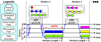
Figure 1: Overview of on-demand CPP

Example 2

In Figure 1, we show a schematic diagram of the on-demand CPP approach for three robots in an arbitrary workspace. In horizon $1$, the CP finds paths of lengths $0,2$, and $3$ for the participants $r^{1},r^{2}$, and $r^{3}$, respectively. Observe that only $r^{2}$ and $r^{3}$ are active. As the horizon length turns out to be $2$, the CP stores the remaining part of $r^{3}$’s path. Now, $r^{2}$ and $r^{3}$ follow their equal-length paths while $r^{1}$ waits. In horizon $2$, however, the CP finds paths only for $r^{1}$ and $r^{2}$ (notice the new colors) as non-participant $r^{3}$ already has its remaining path (notice the same color) found in horizon $1$.

III-A Data structures at CP

Before delving deep into the processes that run at each robot $r^{i}$ (Algorithm 1) and the CP (Algorithm 2), we define the data structures that the CP uses for computation.

Let $\Sigma_{rem}$ denote the set $\{\sigma^{i}_{rem}\,|\,i\in[R]\}$ of remaining paths of all the robots for the next horizon, where $\sigma^{i}_{rem}$ denotes the remaining path for $r^{i}$. Initially, none of the robots has any remaining path, i.e., $\sigma^{i}_{rem}$ is $\mathsf{NULL}$ for each $r^{i}$. We denote the set of indices of the robots participating in the current horizon by $I_{par}\subseteq[R]$ and the number of requests received in the current horizon by $N_{req}\in[R]_{0}$. Also, $N_{act}\in[R]_{0}$ denotes the number of active robots in the current horizon. By $I^{inact}_{par}$, we denote the set of indices of the inactive robots of the previous horizon, and by $S^{inact}$, their start states. So, the CP must incorporate the robots $I^{inact}_{par}$ into the planning of the current horizon. Finally, $\widetilde{W_{g}}$ denotes the goals at which the remaining paths end. So, $\widetilde{W_{g}}$ remains reserved for the corresponding robots, and the CP cannot assign $\widetilde{W_{g}}$ to any other robot hereafter.

III-B Overall On-Demand Coverage Path Planning

In this section, we present the overall on-demand CPP approach in detail. First, we explain Algorithm 1, which runs at the robots’ end. Each robot $r^{i}$ initializes its local view $W^{i}=\langle W^{i}_{u},W^{i}_{o},W^{i}_{g},W^{i}_{c}\rangle$ (line 1), where $W^{i}_{u},W^{i}_{o},W^{i}_{g},$ and $W^{i}_{c}$ are the set of unexplored, obstacle, goal, and covered cells, respectively, due to the partial visibility of the workspace. Subsequently, $r^{i}$ creates a request message $\mathtt{M_{req}[id,state,view]}$ (line 2) and sends that to the CP (line 4) to inform about its local view. Then, $r^{i}$ waits for a response message $\mathtt{M_{res}[path]}$ (line 5) from the CP. Upon receiving, $r^{i}$ extracts its path into $\sigma^{i}$ and starts to follow it (line 6). While following, $r^{i}$ explores newly visible cells and accordingly updates $W^{i}$. Finally, once it reaches the last state $s^{i}_{|\sigma^{i}|}$ of $\sigma^{i}$, it updates its $\mathtt{M_{req}}$ (line 7) to inform the CP about its updated $W^{i}$. The same communication cycle continues between $r^{i}$ and the CP in a while loop (lines 3-7). Here, we assume that the communication medium is reliable and each communication takes negligible time.

1

2

3$W^{i}\leftarrow\mathtt{init\_localview}(s^{i}_{0},X,Y)$

$\mathtt{M_{req}[id,state,view]}\leftarrow[i,s^{i}_{0},W^{i}]$

  // Create $\mathtt{M_{req}}$

4 while true do

5      $\mathtt{send\_localview(M_{req})}$

6      $\sigma^{i}\leftarrow$ $\mathtt{receive\_path(M_{res})}$

7      $W^{i}\leftarrow\mathtt{follow\_path(\sigma^{i})}$

      $\mathtt{M_{req}[state,view]}\leftarrow[s^{i}_{|\sigma^{i}|},W^{i}]$

       // Update $\mathtt{M_{req}}$

8     

Algorithm 1 $\mathtt{Robot}(i,s^{i}_{0},X,Y)$

1

2

3

$\Sigma_{rem}\leftarrow\{\mathsf{NULL}\ |\ i\in[R]\}$

  // Init.

4 $I_{par}\leftarrow\emptyset$, $S\leftarrow\emptyset$, $I^{inact}_{par}\leftarrow\emptyset$, $S^{inact}\leftarrow\emptyset$, $W\leftarrow\emptyset$, $\widetilde{W_{g}}\leftarrow\emptyset$, $\Pi\leftarrow\emptyset$

$N_{req}\leftarrow 0$

  // Number of requests

$N_{act}\leftarrow R$

  // Number of active robots

5 Service receive_localview($\mathtt{M_{req}}$):

      $i\leftarrow\mathtt{M_{req}.id}$

       // Robot ID

6     

7     if $\sigma^{i}_{rem}=\mathsf{NULL}$ then

           $I_{par}\leftarrow I_{par}\cup\{i\}$

            // $r^{i}$ is a participant

8           $S\leftarrow S\cup\{\mathtt{M_{req}.state}\}$

9          

10          

11          $\textnormal{{update\_globalview}}(\mathtt{M_{req}.view})$

12           $N_{req}\leftarrow N_{req}+1$

13          

14          if $(N_{req}=N_{act})$ then

                $I_{par}\leftarrow I_{par}\cup I^{inact}_{par}$

                 // Formerly inactive

15                $S\leftarrow S\cup S^{inact}$

                $\Sigma\leftarrow$ OnDemCPP_Hor ()

                 // Equal-length paths

16                send_paths_to_active_robots ($\Sigma$)

                $I_{par}\leftarrow\emptyset$, $S\leftarrow\emptyset$

                 // Reinit.

17                $N_{req}\leftarrow 0$

18               

19               

20                Function update_globalview($\mathtt{M_{req}.view}$):

                     $W^{i}\leftarrow\mathtt{M_{req}.view}$

                      // Local view of $r^{i}$

21                     for $(x,y)\in W^{i}_{c}$ do

22                          if $(x,y)\notin W_{c}$ then

                               $W_{c}\leftarrow W_{c}\cup\{(x,y)\}$

                                // Covered

23                              

24                              

25                               for $(x,y)\in W^{i}_{g}$ do

26                                    if $(x,y)\in W_{u}$ then

                                         $W_{g}\leftarrow W_{g}\cup\{(x,y)\}$

                                          // Goal

27                                        

28                                        

29                                         $W_{g}\leftarrow W_{g}\setminus W_{c}$

30                                         for $(x,y)\in W^{i}_{o}$ do

31                                              if $(x,y)\in W_{u}$ then

                                                   $W_{o}\leftarrow W_{o}\cup\{(x,y)\}$

                                                    // Obstacle

32                                                  

33                                                  

34                                                   $W_{o}\leftarrow W_{o}\setminus W_{c}$

                                                   $W_{u}\leftarrow([X]\times[Y])\setminus(W_{c}\cup W_{g}\cup W_{o})$

                                                    // Unexplored

35                                                  

36                                                   Function send_paths_to_active_robots($\Sigma$):

37                                                        parallel for $i\in[R]\setminus I^{inact}_{par}$ do

                                                            $\mathtt{M_{res}[path]}\leftarrow\sigma^{i}$

                                                         // Create $\mathtt{M_{res}}$

38                                                             send_path ($\mathtt{M_{res},i}$)

39                                                       

40                                                        Function OnDemCPP_Hor():

                                                             $\Sigma^{\prime}\leftarrow\emptyset$

                                                              // Participants’ collision-free paths

41                                                            

42                                                            if $(W_{g}\setminus\widetilde{W_{g}})\neq\emptyset$ then

43                                                                  $\Sigma^{\prime}\leftarrow\textnormal{{CPPForPar}}(W,\widetilde{W_{g}},I_{par},S,M,R,\Sigma_{rem})$

44                                                                 

45                                                                  else if $I_{par}\neq[R]$ then

46                                                                       for $i\in I_{par}$ do

47                                                                            $\sigma^{\prime i}\leftarrow s^{i}_{0}$

48                                                                            $\Sigma^{\prime}\leftarrow\Sigma^{\prime}\cup\{\sigma^{\prime i}\}$

49                                                                           

50                                                                            else

                                                                                 exit ()

                                                                                  // Coverage Complete !!!

51                                                                                

52                                                                                

53                                                                                $\Sigma^{\prime}_{all}\leftarrow\mathtt{combine\_paths}(I_{par},\Sigma^{\prime},R,\Sigma_{rem})$

54                                                                                 $\lambda\leftarrow\mathtt{determine\_horizon\_length}(\Sigma^{\prime}_{all})$

55                                                                                 $\Sigma\leftarrow$ get_equal_length_paths ($\Sigma^{\prime}_{all},\lambda$)

56                                                                                 return $\Sigma$

57                                                                                

58                                                                                 Function get_equal_length_paths($\Sigma^{\prime}_{all},\lambda$):

59                                                                                      $\Sigma\leftarrow\emptyset$, $\Sigma_{rem}\leftarrow\emptyset$, $\widetilde{W_{g}}\leftarrow\emptyset$, $I^{inact}_{par}\leftarrow\emptyset$, $S^{inact}\leftarrow\emptyset$

                                                                                      $N_{act}\leftarrow 0$

                                                                                       // Reinit.

60                                                                                     

61                                                                                     for $i\in[R]$ do

62                                                                                           if $|\sigma^{\prime i}_{all}|>0$ then

                                                                                                $N_{act}\leftarrow N_{act}+1$

                                                                                                 // $r^{i}$ is active

63                                                                                                $\langle\sigma^{i},\sigma^{i}_{rem}\rangle\leftarrow\mathtt{split\_path}(\sigma^{\prime i}_{all},\lambda)$

64                                                                                                $\Sigma\leftarrow\Sigma\cup\{\sigma^{i}\}$

65                                                                                               

66                                                                                               if $|\sigma^{i}_{rem}|>0$ then

                                                                                                     $\widetilde{W_{g}}\leftarrow\widetilde{W_{g}}\cup\{\mathcal{L}(s^{i}_{|\sigma^{\prime i}_{all}|})\}$

                                                                                                      // Reserve

67                                                                                                    

68                                                                                                     else

69                                                                                                          $\sigma^{i}_{rem}\leftarrow\mathsf{NULL}$

70                                                                                                         

71                                                                                                         

                                                                                                         $\pi^{i}\leftarrow\pi^{i}:\sigma^{i}$

                                                                                                           // Concat.

72                                                                                                         

73                                                                                                          else

                                                                                                               $I^{inact}_{par}\leftarrow I^{inact}_{par}\cup\{i\}$

                                                                                                                // $r^{i}$ is inactive

74                                                                                                               $S^{inact}\leftarrow S^{inact}\cup\{s^{i}_{0}\}$

75                                                                                                               $\sigma^{i}_{rem}\leftarrow\mathsf{NULL}$

                                                                                                               $\pi^{i}\leftarrow\pi^{i}:\mathtt{dummy\_path}(s^{i}_{0},\lambda)$

                                                                                                                // Concat.

76                                                                                                              

77                                                                                                              

78                                                                                                              $\Sigma_{rem}\leftarrow\Sigma_{rem}\cup\{\sigma^{i}_{rem}\}$

79                                                                                                              

80                                                                                                              

81                                                                                                              return $\Sigma$

Algorithm 2 $\mathtt{OnDemCPP}(R,X,Y)$

We now describe Algorithm 2 in detail, which runs at the CP’s end. After initializing the required data structures (lines 1-4), the CP starts a service (lines 5-18) to receive requests from the robots in a mutually exclusive manner. Upon receiving a $\mathtt{M_{req}}$ from $r^{i}$ (line 6), the CP checks whether $r^{i}$ has any remaining path $\sigma^{i}_{rem}$ or not (line 7). If $r^{i}$ has, it does not participate in the planning of the current horizon. Otherwise (lines 7-9), $r^{i}$ participates and so the CP adds $r^{i}$’s ID $\{i\}$ into $I_{par}$, and current state into $S$. In either case, the CP updates the global view of the workspace $W=\langle W_{u},W_{o},W_{g},W_{c}\rangle$ increamentally (line 10).

In update_globalview (lines 19-32), first, the CP extracts the local view $W^{i}$ of $r^{i}$ (line 20). Then, it marks all the cells visited by $r^{i}$ as covered in the global view $W$ (lines 21-23). Next, the CP marks any unexplored cell in $W$ as a goal if $r^{i}$ classifies that cell as a goal (lines 24-26). Similarly, the CP marks any unexplored cell in $W$ as an obstacle if $r^{i}$ classifies that cell as an obstacle (lines 28-30). As $r^{i}$ visits some previously found goals, making them covered, the CP filters out those covered cells from $W_{g}$ (line 27). Also, as a robot cannot distinguish between an obstacle and another robot using the fitted rangefinders, the CP filters out those covered cells from $W_{o}$ that previously posed as obstacles (line 31). Finally, the CP marks the remaining cells in $W$ as unexplored (line 32).

Figure 2: Incremental updation of the global view $W$

Example 3

In Figure 2, we show an example, where two robots, namely $r^{1}$ and $r^{2}$ with initial states $(2,1,\mathtt{W})$ and $(3,1,\mathtt{N})$, respectively, get deployed in a $3\times 3$ workspace. Notice that $r^{2}$ appears as an obstacle to $r^{1}$ in its local view $W^{1}$. Likewise, $r^{1}$ appears as an obstacle to $r^{2}$ in its local view $W^{2}$. Without loss of generality, we assume the CP receives requests from $r^{1}$ first and then from $r^{2}$ and incrementally updates the global view $W$ accordingly.

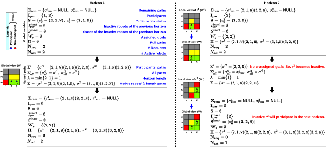
Figure 3: Skip replanning the participants in the current horizon

Once the CP receives all the requests from the active robots of the previous horizon (lines 11-12), it makes the inactive robots of the previous horizon $I^{inact}_{par}$ participants (lines 13-14). Then, it invokes OnDemCPP_Hor (line 15), which does the path planning for the current horizon (we describe in Section III-C). OnDemCPP_Hor updates $I^{inact}_{par}$, which now contains the inactive robots of the current horizon, and returns the equal-length paths $\Sigma$ for the active robots $[R]\setminus I^{inact}_{par}$ of the current horizon. So, the CP simultaneously sends paths to those active robots through response messages $\mathtt{M_{res}}$ (lines 16 and 33-36). Finally, it reinitializes some data structures for the next horizon (lines 17-18).

III-C Coverage Path Planning in the Current Horizon

Here, we describe the rest of Algorithm 2. Recall that the CP has already assigned the goals $\widetilde{W_{g}}$ to the non-participants in some past horizons. In OnDemCPP_Hor (lines 37-50), first, the CP checks whether there are unassigned goals, i.e., $W_{g}\setminus\widetilde{W_{g}}$ left in the workspace (line 39). If so, it attempts to generate the collision-free paths $\Sigma^{\prime}=\{\sigma^{\prime i}\ |\ i\in I_{par}\}$ for the participants $I_{par}$ to visit some unassigned goals while keeping the remaining paths $\Sigma_{rem}$ of the non-participants $[R]\setminus I_{par}$ (hereafter denoted by $\overline{I_{par}}$) intact (line 40). We defer the description of CPPForPar to Section III-D. Otherwise, the CP cannot plan for the participants. Thereby, it skips replanning the participants in the current horizon. Still, if there are non-participants (line 41), they can proceed toward their assigned goals in the current horizon while the participants remain inactive. To signify this, the CP assigns the current states of the participants to their paths $\Sigma^{\prime}$ (lines 42-44). Note that when both the criteria, viz all the robots are participants, and there are no unassigned goals get fulfilled (lines 45-46), it means complete coverage (established in Theorem 1 in Section IV). Next, the CP combines $\Sigma^{\prime}$ with $\Sigma_{rem}$ into $\Sigma^{\prime}_{all}=\{\sigma^{\prime i}_{all}|i\in[R]\}$, where

$$\sigma^{\prime i}_{all}=\begin{cases}\sigma^{\prime i},&\text{if $i\in I_{par}$},\\ \sigma^{i}_{rem},&\text{otherwise}.\end{cases}$$

Thus, $\sigma^{\prime i}_{all}$ contains the collision-free path $\sigma^{\prime i}$ if $r^{i}$ is a participant, otherwise contains the remaining path $\sigma^{i}_{rem}$ of the non-participant $r^{i}$. Notice that $\Sigma^{\prime}_{all}$ contains the collision-free paths for all the robots (line 47). A robot $r^{i}$ is said to be active in the current horizon if its path length is non-zero, i.e., $|\sigma^{\prime i}_{all}|>0$. Otherwise, $r^{i}$ is said to be inactive. In the penultimate step, the CP determines the length of the current horizon (line 48) as the minimum path length of the active robots, i.e., $\lambda=\min_{i\in[R]}\{|\sigma^{\prime i}_{all}|>0\}$. Finally, it returns $\lambda$-length paths $\Sigma$ only for the active robots (lines 49-50). This way, the CP ensures that at least one active robot (participant or non-participant) reaches its goal in the current horizon.

In $\mathtt{get\_equal\_length\_paths}$ (lines 51-70), after re-initialization of some of the data structures (lines 52-53), the CP examines the paths $\Sigma^{\prime}_{all}$ in a for loop (lines 54-69) to determine which robots are active (lines 55-63), and which are not (lines 64-68). If $r^{i}$ is active, first, the CP increments $N_{act}$ by $1$ (line 56). Then, the CP splits its path $\sigma^{\prime i}_{all}$ into two parts $\sigma^{i}$ and $\sigma^{i}_{rem}$ of lengths $\lambda$ and $|\sigma^{\prime i}_{all}|-\lambda$, respectively (line 57). Active $r^{i}$ traverses the former part $\sigma^{i}$, containing $s^{i}_{0}\ldots s^{i}_{\lambda}$, in the current horizon (line 58) and the later part (if any), containing $s^{i}_{\lambda}\ldots s^{i}_{|\sigma^{\prime i}_{all}|}$, in the future horizons (line 69). If it has the remaining path $\sigma^{i}_{rem}$, its goal location $\mathcal{L}(s^{i}_{|\sigma^{\prime i}_{all}|})$ gets added to $\widetilde{W_{g}}$ (lines 59-60), signifying that this goal remains reserved for $r^{i}$. Otherwise, $\sigma^{i}_{rem}$ is set to $\mathsf{NULL}$ (lines 61-62 and 69), indicating the absence of the remaining path for $r^{i}$, thereby enabling $r^{i}$ to become a participant in the next horizon. In contrast, if $r^{i}$ is inactive (lines 64-68), the CP adds $r^{i}$’s ID $\{i\}$ and its start state $s^{i}_{0}$ into $I^{inact}_{par}$ and $S^{inact}$, respectively (lines 65-66), as it would reattempt to find $r^{i}$’s path in the next horizon. The CP also sets $\sigma^{i}_{rem}$ to $\mathsf{NULL}$ (lines 67 and 69). Note that the CP also generates the full path for the active robots (line 63) and the inactive robots (line 68), where $\mathtt{dummy\_paths}$ generates a path of length $\lambda$ containing only the current state. The CP sends no path to an inactive robot in the current horizon (lines 34-36). So, the active robots of the current horizon send requests in the next horizon (lines 56 and 11-12).

Example 4

In Figure 3, we show an example (continuation of Example 3) where the CP skips planning for a participant due to the unavailability of an unassigned goal. In horizon $1$, both the robots $r^{1}$ and $r^{2}$ participate, and the CP finds their collision-free paths $\sigma^{\prime 1}$ and $\sigma^{\prime 2}$ of lengths $2$ and $1$, respectively. Note that both robots are active. As the horizon length ($\lambda$) is found to be $1$, the CP reserves $r^{1}$’s goal into $\widetilde{W_{g}}$, and sets its remaining path $\sigma^{1}_{rem}$ accordingly. Each robot follows its $1$-length path and sends the updated local view to the CP. In horizon $2$, though the CP receives $2$ requests, only $r^{2}$ participates. As no unassigned goal exists (i.e., $W_{g}\setminus\widetilde{W_{g}}=\emptyset$), the CP fails to find any path for $r^{2}$. So, $r^{2}$ becomes inactive, and the CP adds its ID into $I^{inact}_{par}$ and state into $S^{inact}$ as it would reattempt in horizon $3$. Now, only $r^{1}$ (non-participant) is active. As $\lambda$ is found to be $1$, $r^{1}$ visits its reserved goal, which the CP removes from $\widetilde{W_{g}}$ and resets $\sigma^{1}_{rem}$. Notice that in horizon $3$, the CP receives only $1$ request (from $r^{1}$ only), but both the robots participate.

III-D Coverage Path Planning for the Participants

In detail, we now present CPPForPar (Algorithm 3), which in every invocation, generates the collision-free paths only for the participants without altering the remaining paths for the non-participants. It is a modified version of Algorithms 2 and 3 of [44] combined, which uses the idea of Goal Assignment-based Prioritized Planning to generate the collision-free paths for all the robots. Let $R^{*}$ and $G^{*}$ be the number of participants and unassigned goals in the current horizon. So, $R^{*}=|I_{par}|=|S|$ and $G^{*}=|W_{g}\setminus\widetilde{W_{g}}|$. The problem of optimally visiting $G^{*}$ unassigned goals with $R^{*}$ participants is a Multiple Traveling Salesman Problem [56], which is NP-hard. Hence, it is computationally costly when $R^{*}$, $G^{*}$, or both are large. So, the CP generates the participants’ paths in two steps without guaranteeing optimality. First, it assigns the participants to the unassigned goals in a cost-optimal way and finds their optimal paths (line 1 and Algorithm 4). Then, if needed, it makes those optimal paths collision-free by adjusting them using a greedy method (line 2 and Algorithm 5), thereby may lose optimality.

1

2

Result: Collision-free paths for the participants $(\Sigma^{\prime})$

3

4$\langle\Gamma,\ \Phi\rangle\leftarrow\textnormal{{COPForPar}}(W,\widetilde{W_{g}},I_{par},S,M)$

5 $\Sigma^{\prime}\leftarrow\textnormal{{CFPForPar}}(\Gamma,\Phi,I_{par},R,\Sigma_{rem})$

Algorithm 3 $\mathtt{CPPForPar}(W,\widetilde{W_{g}},I_{par},S,M,R,\Sigma_{rem})$

1

2

Result: Opt. assignment ($\Gamma$) and corresponding paths $(\Phi)$

3

4$\langle\Delta,L_{\Delta}\rangle\leftarrow\mathtt{compute\_optimal\_costs}(W,\widetilde{W_{g}},I_{par},S,M)$

5 $\Gamma\leftarrow\mathtt{compute\_optimal\_assignments}(\Delta,I_{par})$

6 $\Phi\leftarrow\mathtt{get\_optimal\_paths}(L_{\Delta},\Gamma,I_{par})$

Algorithm 4 $\mathtt{COPForPar}(W,\widetilde{W_{g}},I_{par},S,M)$

III-D1 Sum-of-Costs-optimal goal assignment and corresponding paths

First, we construct a weighted state transition graph $\mathcal{G}_{\Delta}$. Its vertices $\mathcal{G}_{\Delta}.V$ are the all possible states of the participants s.t. $\mathcal{L}(s)\in W_{g}\cup W_{c}$, $\forall s\in\mathcal{G}_{\Delta}.V$. And its edges $\mathcal{G}_{\Delta}.E$ are the all possible transitions among the states, i.e., $e(s^{\prime},s^{\prime\prime})\in\mathcal{G}_{\Delta}.E$ iff $s^{\prime},s^{\prime\prime}\in\mathcal{G}_{\Delta}.V$ and $\exists\mu\in M$ s.t. $s^{\prime}\xrightarrow{\mu}s^{\prime\prime}$. Moreover, the weight of an edge $e$ is $\mathtt{cost}(\mu)$. Now, for each pair of participant $r^{i}$ (i.e., $i\in I_{par}$) and unassigned goal $\gamma^{j}\in W_{g}\setminus\widetilde{W_{g}}$ (i.e., $j\in[G^{*}]$), we run the A* algorithm [57, 58] to compute the optimal path that originates from the start state $s^{i}_{0}$ and terminates at the state $s$ s.t. $\mathcal{L}(s)=\gamma^{j}$. We store the cost of the path in $\Delta[i][j]\in\mathbb{R}$, and the corresponding path in $L_{\Delta}[i][j]$ (line 1 of Algorithm 4). Next, we apply the Hungarian algorithm [59, 60] on $\Delta$ to find the cost-optimal assignment $\Gamma:I_{par}\rightarrow[G^{*}]\cup\{\mathsf{NULL}\}$ (line 2), signifying which participant would go to which unassigned goal. Notice that some participants would get assigned $\mathsf{NULL}$ when $R^{*}>G^{*}$. We call such participants inactive and the rest of the participants active. Finally, for each participant $r^{i}$, its optimal path $\varphi^{i}\in\Phi$ is set to $L_{\Delta}[i][j]$ if $\Gamma[i]=j$, otherwise (i.e., when participant $r^{i}$ is inactive), set to its start state $s^{i}_{0}$ (line 3). Thus, we get the set of optimal paths for the participants $\Phi=\{\varphi^{i}\ |\ i\in I_{par}\}$. Keep in mind that the non-participants $\overline{I_{par}}$ are inherently active as their remaining paths $\sigma^{k}_{rem}\neq\mathsf{NULL},\forall k\in\overline{I_{par}}$.

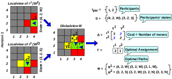
Figure 4: Cost-optimal goal assignment and optimal paths

Example 5

We show an example of cost-optimal goal assignment and corresponding optimal paths in Figure 4 involving two participants $r^{1}$ and $r^{2}$ in a $4\times 4$ workspace.

1

2

Result: Collision-free paths for the participants $(\Sigma^{\prime})$

3

4while $true$ do

5      $\langle\Gamma,\Omega\rangle\leftarrow\mathtt{get\_feasible\_paths}(\Gamma,\Phi,I_{par})$

6      $\Theta_{r}\leftarrow\mathtt{compute\_relative\_precedences}(\Omega,I_{par})$

7      $\Theta_{a}\leftarrow\mathtt{compute\_absolute\_precedence}(\Theta_{r},I_{par})$

8     

9     if $\Theta_{a}$ is valid then

           $\Gamma^{\prime}=\Gamma$

            // Itemwise copy

10           $\langle\Gamma,\Upsilon\rangle\leftarrow\mathtt{compute\_sto}(\Gamma,\Omega,\Theta_{a},I_{par},R,\Sigma_{rem})$

11          

12          if $\Gamma^{\prime}=\Gamma$ then  break

13          

14           else

15                $\Gamma\leftarrow\mathtt{break\_precedence\_cycles}(\Gamma,\Theta_{r},I_{par})$

16               

17               

18               $\Phi\leftarrow\mathtt{adjust\_paths}(\Gamma,\Omega,I_{par})$

19               

20               

21               $\Sigma^{\prime}\leftarrow\mathtt{get\_collision\_free\_paths}(\Omega,\Upsilon,I_{par})$

Algorithm 5 $\mathtt{CFPForPar}(\Gamma,\Phi,I_{par},R,\Sigma_{rem})$

III-D2 Prioritization

Prioritization is an inter-robot collision-avoidance mechanism, which assigns priorities to the robots either statically (e.g., [61, 62]) or dynamically (e.g., [63, 64]) so that a CP can subsequently find their collision-free paths in order of their priority. In CFPForPar (Algorithm 5), prioritization of the participants $I_{par}$ takes place (in the while loop in lines 1-11 except the if block in lines 5-8) based on the movement constraints among their paths in $\Phi$. But, prioritization surely fails if there is any infeasible path in $\Phi$. So, detection and correction of the infeasible paths are necessary (line 2). There are two types of infeasible paths, namely crossover paths and nested paths. Optimal paths $\varphi^{i}$ and $\varphi^{j}$, where $\varphi^{i},\ \varphi^{j}\in\Phi$, of distinct participants $r^{i}$ and $r^{j}$, where $i,\ j\in I_{par}$, are said to be -

1. a crossover path pair if one of the participants is inactive, which sits on the path of the other active participant, or their start locations are on each other’s path, and

2. a nested path pair if the active participant $r^{i}$’s start and goal locations are on $\varphi^{j}$ of the active participant $r^{j}$, or vice versa.

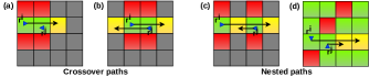
Figure 5: Infeasible paths

Example 6

We show four simple examples of infeasible paths involving two participants $r^{i}$ and $r^{j}$ in Figure  5.

The CP can modify the paths $\Phi$ of the participants, but not the remaining paths $\Sigma_{rem}$ of the non-participants. So, first, we mark those active participants as killed, which form infeasible path pairs with an inactive, active, or already killed participant. In the revival step, we initially mark all the inactive and the killed participants as unrevived. Then, each path $\varphi^{i}$ of the killed participants is processed in reverse until an unrevived participant $r^{j}$ gets found. If $r^{j}$ can reach $r^{i}$’s goal by following $\omega^{j}\in\Omega$ (note that $\omega^{j}$ gets generated from $\varphi^{i}$) without forming any infeasible path pair, then $r^{j}$ gets revived. Thus, a greedy procedure (a modified version of Algorithm 4 in [44], which works only for $R$ participants) generates the feasible paths $\Omega=\{\omega^{i}\ |\ i\ \in\ I_{par}\}$ for the participants through goal reassignments.

Example 7

As a continuation of Example 6, in Figure  5, only $r^{i}$ is an active participant in (a) while both $r^{i}$ and $r^{j}$ are active participants in the rest (b-d). Due to infeasible paths, only $r^{i}$ gets killed in (a) while both $r^{i}$ and $r^{j}$ get killed in the rest (b-d). Though only $r^{j}$ gets revived in (a, c-d), both $r^{i}$ and $r^{j}$ get revived in (b).

Next, for each pair of distinct participants $r^{i}$ and $r^{j}$, we compute the relative precedence $\Theta_{r}[i][j]\in\mathbb{B}$ (line 3) based on their paths $\omega^{i}$ and $\omega^{j}$, respectively, where $\omega^{i},\omega^{j}\in\Omega$. $\Theta_{r}[i][j]$ is set to $1$ if $r^{i}$ must move before $r^{j}$, which is necessary when either the start location of $r^{i}$ is on $\omega^{j}$, or the goal location of $r^{j}$ is on $\omega^{i}$, $0$ otherwise. Similarly, we compute $\Theta_{r}[j][i]$. Finally, we apply the topological sorting on $\Theta_{r}$ to get the absolute precedence $\Theta_{a}$ (line 4). But, it fails if there is any cycle of relative precedence (see Example 8). In that case, we use [65, 66] to get a Directed Acyclic Graph (DAG) out of that Directed Cyclic Graph (DCG) by inactivating some active participants in $\Gamma$ and adjusting their feasible paths $\Omega$ accordingly (lines 9-11), which in turn may form new crossover paths. Therefore, we reexamine the paths in another iteration of the while loop (line 1).

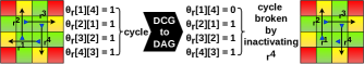
Figure 6: Removal of cyclic precedence

Example 8

In Figure  6, we show an example of removing a precedence cycle involving four participants.

Example 9

As a continuation of Example 5, the feasible paths $\omega^{1}$ and $\omega^{2}$ for the participants $r^{1}$ and $r^{2}$ are same as $\varphi^{1}$ and $\varphi^{2}$, respectively. Also, $\Theta_{r}[2][1]=1$ because $\mathcal{L}(s^{2}_{0})$ is on $\omega^{1}$. Therefore, robot ID $2$ comes before $1$ in $\Theta_{a}$.

III-D3 Time parameterization

Time parameterization ensures inter-robot collision avoidance through decoupled planning. Recall that the CP does not change the remaining paths $\Sigma_{rem}$ for the non-participants, implicitly meaning the non-participants have higher priorities than the participants. So, for each participant $r^{i}$ in order of $\Theta_{a}$, we incrementally compute its start time offset $\Upsilon[i]\in\mathbb{N}_{0}$ (line 7). It is the amount of time $r^{i}$ must wait at its start state to avoid collisions with its higher priority robots (some other participants and the non-participants). But, a collision between a participant $r^{i}$ and non-participant $r^{j}$ may become inevitable (see Example 11). In that case, the CP inactivates the participant in $\Gamma$ and reexamines updated paths $\Phi$ (line 11) for the presence of new crossover paths. In the worst case, all the participants may get inactivated due to inevitable collisions with the non-participants. Otherwise, $r^{i}$’s collision-free path $\sigma^{\prime i}\in\Sigma^{\prime}$ gets generated (line 12) by inserting its start state $s^{i}_{0}$ at the beginning of $\omega^{i}$ for $\Upsilon[i]$ times.

Example 10

As a continuation of Example 9, start time offsets for the participants $r^{2}$ is $\Upsilon[2]=0$, and $r^{1}$ is $\Upsilon[1]=2$ because any value smaller than $2$ would cause a collision. Therefore, the collision-free path lengths for the participants $r^{1}$ and $r^{2}$ are $|\sigma^{\prime 1}|=4$ and $|\sigma^{\prime 2}|=3$, respectively. Observe that the horizon length $\lambda=3$.

Figure 7: Inactivation of a participant during offsetting

Example 11

In Figure 7, we show an extreme case of replanning where the CP inactivates a participant to avoid collision with a non-participant. Notice that both the robots $r^{1}$ and $r^{2}$ have traversed their full paths of length five till horizon $4$. In horizon $5$, both participate because none has any remaining path. The CP assigns the unassigned goal ids $2$ and $1$ to $r^{1}$ and $r^{2}$, respectively, and subsequently finds their collision-free paths $\Sigma^{\prime}$. As the horizon length ($\lambda$) is found to be $2$, the CP reserves the goal $(3,\ 2)$ for $r^{1}$ in $\widetilde{W_{g}}$ and sets its remaining path $\sigma^{1}_{rem}$ accordingly. Therefore, only $r^{2}$ participates in horizon $6$. The CP finds $r^{2}$’s optimal path $\varphi^{2}$ leading to the only unassigned goal $(4,\ 2)$. Though the prioritization succeeds trivially, the offsetting fails because the non-participant $r^{1}$ would reach its goal $(3,\ 2)$ before the participant $r^{2}$ gets past that goal. So, the CP inactivates $r^{2}$. In this horizon, only $r^{1}$ remains active with $\lambda=1$. Observe that both will participate in the next horizon.

IV Theoretical Analysis

First, we formally prove that OnDemCPP covers $W$ completely and then analyze its time complexity.

IV-A Proof of Complete Coverage

Lemma 1 (Lemma $4.3$ of [44])

GAMRCPP_Horizon ensures that at least one goal gets visited in each horizon.

Lemma 2

CPPForPar $\equiv$ GAMRCPP_Horizon if $R^{*}=R$.

Proof:

When all the robots are participants, i.e., $R^{*}=R$, there are no non-participants, i.e., $\overline{I_{par}}=\emptyset$. It implies that in $\Sigma_{rem}$, $\sigma^{i}_{rem}=\mathsf{NULL},\forall i\in[R]$, thereby $\widetilde{W_{g}}=\emptyset$. Hence, CPPForPar $\equiv$ GAMRCPP_Horizon if $R^{*}=R$. ∎

Lemma 3

OnDemCPP_Hor ensures that at least one robot visits its goal in each horizon.

Proof:

The set of all collision-free paths $\Sigma^{\prime}_{all}$ (line 47 of Algorithm 2) consists of two kinds of paths, namely the paths $\Sigma^{\prime}$ of the participants $I_{par}$ and the remaining paths $\Sigma_{rem}$ of the non-participants $\overline{I_{par}}$. Now, consider two cases: (1) $R^{*}=R$ and (2) $R^{*}<R$. In the case of (1), $\widetilde{W_{g}}=\emptyset$. Further, by Lemma 2 and Lemma 1, when $W_{g}\neq\emptyset$ (lines 39-40), there is at least one active robot in $\Sigma^{\prime}$, and so in $\Sigma^{\prime}_{all}$. In the case of (2), however, $\widetilde{W_{g}}\neq\emptyset$ because there are $R-R^{*}$ non-participants. Thus, $\Sigma^{\prime}_{all}$ contains at least one active robot because the non-participants are active. Moreover, the horizon length $\lambda$ (line 48) ensures that at least one robot (participant or non-participant) remains active in the $\lambda$-length paths $\Sigma$ (line 49) to visit its goal. ∎

Theorem 1

OnDemCPP eventually terminates, and when it does, it ensures complete coverage of $W$.

Proof:

By Lemma 3, in a horizon, at least one active robot visits its goal, thereby exploring $W_{u}$ (as $W_{free}$ is strongly connected) and adding new goals (if any) into $W_{g}$. If an active participant visits its goal, the CP marks that goal as covered. So, in the next horizon, $W_{g}$ decreases, and $W_{c}$ increases. But, if a non-participant (inherently active) visits its goal, the CP removes that reserved goal from $\widetilde{W_{g}}$ in the next horizon, thereby decreasing $\widetilde{W_{g}}$. But, it may not increase $W_{c}$ as other robots might have already passed through that goal in the past horizons, already covering it in $W_{c}$. These two types of active robots and the inactive participants $I^{inact}_{par}$ participate in the next horizon (line 13 of Algorithm 2). However, the rest of the active robots who cannot visit their goals in the current horizon become non-participants in the next horizon as the CP reserves their goals into $\widetilde{W_{g}}$. Each reserved goal in $\widetilde{W_{g}}$ gets visited eventually in some horizon (as the CP does not alter the corresponding robot’s remaining path), making the corresponding robot participant in the next horizon. Therefore, eventually, all the robots become participants (i.e., $I_{par}=[R]$), falsifying the if condition (line 41), and hence $\widetilde{W_{g}}=\emptyset$. Now, if $W_{g}=\emptyset$ (line 39), it entails $W_{c}=W_{free}$ (lines 45-46). ∎

Note that OnDemCPP can also ensure complete coverage of a $W$, where $W_{free}$ is not strongly connected, provided we deploy at least one robot in each component.

IV-B Time Complexity Analysis

Lemma 4

CFPForPar takes $\mathcal{O}(R^{3})$.

Proof:

The only difference between CFPForPar (Algorithm 5) and $\mathtt{GAMRCPP\_CFP}$ (Algorithm 3 in [44]) is that $\mathtt{compute\_sto}$ (line 7 of Algorithm 5) gets called just after the while loop in $\mathtt{GAMRCPP\_CFP}$. Still, the time complexity of $\mathtt{compute\_sto}$ and the rest of the body of the while loop (lines 1-11 of Algorithm 5) remain $\mathcal{O}(R^{3})$ (interested reader may read Theorem 4.6 of [44]) as $R^{*}=\mathcal{O}(R)$. ∎

Lemma 5

CPPForPar takes $\mathcal{O}(|W|^{3})$.

Proof:

CPPForPar (Algorithm 3) does the task performed by lines 1-4 of GAMRCPP_Horizon (Algorithm 2 in [44]). Therefore, CPPForPar takes as much time as GAMRCPP_Horizon, which is $\mathcal{O}(|W|^{3})$ (interested reader may read Theorem 4.6 of [44]). ∎

Lemma 6

OnDemCPP_Hor takes $\mathcal{O}(|W|^{3})$.

Proof:

Finding the unassigned goals $W_{g}\setminus\widetilde{W_{g}}$ (line 39 of Algorithm 2) takes $\mathcal{O}(|W|)$ as both $W_{g}$ and $\widetilde{W_{g}}$ are bounded by $\mathcal{O}(|W|)$. As per Lemma  5, CPPForPar (line 40) takes $\mathcal{O}(|W|^{3})$. Checking the existence of non-participants (line 41) takes $\mathcal{O}(R)$. The generation of the zero-length paths for the participants (lines 42-44) takes $\mathcal{O}(R^{*})$. Combining all the paths into $\Sigma^{\prime}_{all}$ (line 47) and determining the horizon length $\lambda$ (line 48) take $\mathcal{O}(R)$. Subsequently, generating the $\lambda$-length paths $\Sigma$ (lines 49 and 51-70) take $\mathcal{O}(R)$ as the for loop in get_equal_length_paths (lines 54-69) takes $\mathcal{O}(R)$. So, OnDemCPP_Hor takes $\mathcal{O}((|W|+|W|^{3})+(R+R^{*})+3\cdot R)$, which can be written as $\mathcal{O}(|W|^{3})$ as $R=\mathcal{O}(|W|)$. ∎

Theorem 2

OnDemCPP’s time complexity is $\mathcal{O}(|W|^{4})$.

Proof:

Each call to update_globalview (line 10 of Algorithm 2) takes $\mathcal{O}(|W|^{2})$ as follows: three for loops (lines 21-23, 24-26, and 28-30) and computing $W_{g},\ W_{o}$, and $W_{u}$ (lines 27, 31-32) take $\mathcal{O}(|W|^{2})$. In a horizon, $N_{req}=\mathcal{O}(R)$ (line 11). So, update_globalview total takes $\mathcal{O}(R\cdot|W|^{2})$, which is $\mathcal{O}(|W|^{3})$. According to Lemma  3, at least one robot visits its goal in each horizon. In the worst case, in each horizon, only one robot visits its goal while the rest remains inactive or makes progress toward their goals. As the number of horizons is at most $|W_{g}|$, the service receive_localview invokes OnDemCPP_Hor (line 15) at most $|W_{g}|$ times. So, OnDemCPP takes $\mathcal{O}(|W_{g}|\cdot(|W|^{3}+|W|^{3}))$, which is $\mathcal{O}(|W|^{4})$. ∎

V Evaluation

TABLE I: Experimental results

					$T_{c}\ ($\mathrm{s}$)$		$T_{p}\ ($\mathrm{s}$)$		$T_{m}\ ($\mathrm{s}$)$		Mission
$M$	Workspace		$R$	$R^{*}$	GAMRCPP	OnDemCPP	GAMRCPP	OnDemCPP	GAMRCPP	OnDemCPP	speed up
Quadcopter	W1: w_woundedcoast $578\times 642$ (34,020)		128	080.4 (62.9 %) $\pm$ 3.8	619.5 $\pm$ 097.9	362.2 $\pm$ 058.4	696.2 $\pm$ 55.5	1042.0 $\pm$ 149.5	1315.7 $\pm$ 148.6	1404.2 $\pm$ 167.1	0.9
			256	170.7 (66.7 %) $\pm$ 5.7	1091.3 $\pm$ 255.3	521.7 $\pm$ 150.2	416.8 $\pm$ 95.0	804.2 $\pm$ 250.9	1508.1 $\pm$ 345.3	1325.9 $\pm$ 383.0	1.1
			512	361.5 (70.6 %) $\pm$ 9.7	1815.2 $\pm$ 359.4	569.1 $\pm$ 168.6	231.8 $\pm$ 33.0	557.2 $\pm$ 138.9	2047.0 $\pm$ 388.0	1126.3 $\pm$ 255.4	1.8
	W2: Paris_1_256 $256\times 256$ (47,240)		128	081.3 (63.6 %) $\pm$ 2.6	513.5 $\pm$ 038.4	270.4 $\pm$ 037.8	815.2 $\pm$ 77.4	962.6 $\pm$ 100.8	1328.7 $\pm$ 109.8	1233.0 $\pm$ 118.8	1.1
			256	157.2 (61.4 %) $\pm$ 3.7	1461.9 $\pm$ 164.0	537.2 $\pm$ 079.6	508.0 $\pm$ 22.0	656.2 $\pm$ 049.4	1969.9 $\pm$ 172.2	1193.4 $\pm$ 110.8	1.7
			512	335.6 (65.6 %) $\pm$ 7.0	3338.8 $\pm$ 321.9	894.0 $\pm$ 113.6	301.1 $\pm$ 19.2	455.7 $\pm$ 050.1	3639.9 $\pm$ 333.6	1349.7 $\pm$ 117.1	2.7
	W3: Berlin_1_256 $256\times 256$ (47,540)		128	083.2 (65.1 %) $\pm$ 2.5	489.3 $\pm$ 036.5	238.4 $\pm$ 017.2	752.7 $\pm$ 032.6	898.2 $\pm$ 063.9	1242.0 $\pm$ 067.4	1136.6 $\pm$ 065.0	1.1
			256	167.4 (65.4 %) $\pm$ 12.1	1323.9 $\pm$ 154.2	515.2 $\pm$ 069.8	564.6 $\pm$ 132.5	669.6 $\pm$ 048.9	1888.5 $\pm$ 234.1	1184.8 $\pm$ 103.3	1.6
			512	365.2 (71.3 %) $\pm$ 34.5	3196.5 $\pm$ 329.4	856.0 $\pm$ 115.1	434.5 $\pm$ 209.9	524.9 $\pm$ 140.0	3631.0 $\pm$ 434.1	1380.9 $\pm$ 238.9	2.6
	W4: Boston_0_256 $256\times 256$ (47,768)		128	079.6 (62.2 %) $\pm$ 4.5	509.5 $\pm$ 036.4	250.6 $\pm$ 030.1	773.6 $\pm$ 61.7	928.0 $\pm$ 100.6	1283.1 $\pm$ 094.0	1178.6 $\pm$ 116.3	1.1
			256	157.8 (61.7 %) $\pm$ 9.3	1220.1 $\pm$ 215.0	455.7 $\pm$ 061.2	460.3 $\pm$ 44.8	625.9 $\pm$ 046.9	1680.4 $\pm$ 256.8	1081.6 $\pm$ 092.4	1.6
			512	345.3 (67.5 %) $\pm$ 7.7	2454.7 $\pm$ 525.7	628.7 $\pm$ 119.3	252.9 $\pm$ 23.5	428.7 $\pm$ 069.2	2707.6 $\pm$ 546.1	1057.4 $\pm$ 182.2	2.6
TurtleBot	W5: maze-128-128-2 $128\times 128$ (10,858)		128	075.5 (59.0 %) $\pm$ 7.4	90.8 $\pm$ 19.3	49.5 $\pm$ 19.8	451.9 $\pm$ 71.7	791.5 $\pm$ 202.1	542.7 $\pm$ 88.6	841.0 $\pm$ 217.7	0.6
			256	174.7 (68.3 %) $\pm$ 7.5	193.6 $\pm$ 27.1	68.1 $\pm$ 16.9	218.6 $\pm$ 35.6	417.6 $\pm$ 097.4	412.2 $\pm$ 58.7	485.7 $\pm$ 113.7	0.8
			512	378.4 (73.9 %) $\pm$ 6.8	411.1 $\pm$ 64.7	124.1 $\pm$ 23.9	125.9 $\pm$ 24.8	224.3 $\pm$ 032.1	537.0 $\pm$ 71.1	348.4 $\pm$ 054.1	1.5
	W6: den520d $257\times 256$ (28,178)		128	071.9 (56.2 %) $\pm$ 3.2	341.8 $\pm$ 050.5	147.6 $\pm$ 17.7	556.4 $\pm$ 71.4	773.1 $\pm$ 106.9	898.2 $\pm$ 121.2	920.7 $\pm$ 117.7	1.0
			256	153.8 (60.1 %) $\pm$ 3.7	685.4 $\pm$ 121.5	253.9 $\pm$ 63.1	324.2 $\pm$ 56.5	506.4 $\pm$ 057.4	1009.6 $\pm$ 175.2	760.3 $\pm$ 103.4	1.3
			512	331.1 (64.7 %) $\pm$ 6.6	1292.4 $\pm$ 304.0	316.0 $\pm$ 29.2	188.7 $\pm$ 09.2	398.6 $\pm$ 037.9	1481.1 $\pm$ 301.9	714.6 $\pm$ 051.7	2.1
	W7: warehouse-20-40-10-2-2 $164\times 340$ (38,756)		128	081.2 (63.5 %) $\pm$ 2.6	467.1 $\pm$ 040.0	211.3 $\pm$ 22.2	595.6 $\pm$ 43.1	707.6 $\pm$ 082.5	1062.7 $\pm$ 075.2	918.9 $\pm$ 098.3	1.2
			256	149.3 (58.3 %) $\pm$ 8.1	1009.5 $\pm$ 165.2	336.0 $\pm$ 31.2	361.6 $\pm$ 25.2	502.5 $\pm$ 078.2	1371.1 $\pm$ 185.3	838.5 $\pm$ 100.4	1.6
			512	335.5 (65.5 %) $\pm$ 7.2	1646.2 $\pm$ 343.7	394.7 $\pm$ 36.6	208.9 $\pm$ 18.0	375.2 $\pm$ 029.5	1855.1 $\pm$ 357.5	769.9 $\pm$ 054.7	2.4
	W8: brc202d $481\times 530$ (43,151)		128	065.1 (50.9 %) $\pm$ 3.5	1019.0 $\pm$ 160.9	395.2 $\pm$ 070.7	915.9 $\pm$ 116.4	1444.9 $\pm$ 232.0	1934.9 $\pm$ 274.3	1840.1 $\pm$ 273.6	1.1
			256	142.0 (55.5 %) $\pm$ 8.7	1880.7 $\pm$ 275.0	697.7 $\pm$ 152.3	512.5 $\pm$ 060.8	972.5 $\pm$ 147.1	2393.2 $\pm$ 326.5	1670.2 $\pm$ 230.3	1.4
			512	309.6 (60.5 %) $\pm$ 9.5	3026.8 $\pm$ 326.8	705.6 $\pm$ 112.5	302.6 $\pm$ 021.6	780.9 $\pm$ 098.5	3329.4 $\pm$ 322.3	1486.5 $\pm$ 163.1	2.2

V-A Implementation and Experimental Setup

We implement Robot (Algorithm 1) and OnDemCPP (Algorithm 2) in a common ROS [67] package and run it in a computer having Intel^® Core^™ i7-4770 CPU @ 3.40 GHz and 16 GB of RAM. For experimentation, we consider eight large $2$D grid benchmark workspaces from [68] of varying size and obstacle density. In each workspace, we incrementally deploy $R\in\{128,256,512\}$ robots and repeat each experiment $10$ times with different initial deployments of the robots to report their mean in the performance metrics (standard deviations are available in [69]).

V-A1 Robots for evaluation

We consider both TurtleBot (introduced before) and Quadcopter in the experimentation. A Quadcopter’s state $s^{i}_{j}=(x,y)\in W$ is its location in the workspace. Its set of motion primitives $M$ = {$\mathtt{Halt(H)}$, $\mathtt{MoveEast(ME)}$, $\mathtt{MoveNorth(MN)}$, $\mathtt{MoveWest(MW)}$, $\mathtt{MoveSouth(MS)}$}, where $\mathtt{ME,MN,MW}$, and $\mathtt{MS}$ move it to the immediate east, north, west, and south cell, respectively.

V-A2 Evaluation metrics

We compare OnDemCPP with GAMRCPP [44] in terms of the mission time ($T_{m}$), which is the sum of the total computation time ($T_{c}$) and the total path execution time ($T_{p}$) while ignoring the total communication time between the CP and the robots. Total computation time ($T_{c}$) is the sum of the computation times spent on OnDemCPP_Hor across all horizons. Total path execution time ($T_{p}$) can be expressed as $T_{p}=\Lambda\times\tau$, where $\Lambda$ is the total horizon length (i.e., the sum of the horizon lengths). We can also express $T_{p}$ as the sum of $T_{Halt}$ and $T_{non-Halt}$, where $T_{Halt}$ is the duration for which the robots remain stationary while following respective paths, i.e., when they execute $\mathtt{Halt(H)}$ moves, and $T_{non-Halt}$ is the duration for which the robots move, i.e., when they do not.

In our evaluation, we take the path cost as the number of moves the corresponding robot performs, where each move takes $\tau=1$\mathrm{s}$$. This is realistic because the maximum transnational velocity of a TurtleBot2 is $0.65$\mathrm{m}$/$\mathrm{s}$$ [55] and that of a Quadcopter is $\sim$ $16$\mathrm{m}$/$\mathrm{s}$$ [70]. Thus, to ensure $\tau=1$\mathrm{s}$$, we can keep the grid cell size for a TurtleBot2 up to $0.65$\mathrm{m}$$, which is sufficient considering its size. Similarly, the grid cell size up to $16$\mathrm{m}$$ is sufficient for most practical applications involving Quadcopters. We demonstrate this in the real experiments described in Section V-C.

V-B Results and Analysis

We show the experimental results in Table I, where we list workspaces in increasing order of their obstacle-free cell count $|W_{free}|$ for each type of robot. In the table, $R^{*}$ denotes the average number of participants over all horizons.

V-B1 Effects of the non-participants on the participants

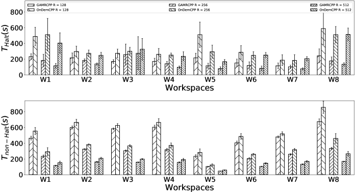
Figure 8: Decomposition of $T_{p}$ into $T_{Halt}$ and $T_{non-Halt}$

Recall that the CP keeps the goals $\widetilde{W_{g}}$ reserved for the non-participants $\overline{I_{par}}$ in a horizon. So, the CP cannot assign these reserved goals to the participants $I_{par}$ in COPForPar (Algorithm 4) even if some participants can visit some reserved goals in a more cost-optimal manner than their corresponding non-participants. Consequently, the CP assigns the participants to the unreserved goals $W_{g}\setminus\widetilde{W_{g}}$, which could be far away. Thus, the particpants’ optimal paths $\Phi$, consisting of non-$\mathtt{Halt}$ moves, become marginally longer in OnDemCPP as $T_{non-Halt}$ justifies in Figure 8.

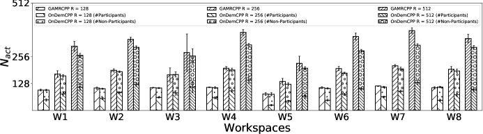
Figure 9: The number of active robots ($N_{act}$) per horizon

Also, recall that the CP does not change the non-participants’ remaining paths $\Sigma_{rem}$ in a horizon. So, it makes the particpants’ optimal paths $\Phi$ inter-robot collision-free in CFPForPar (Algorithm 5) by either prefixing the optimal paths with offsets (i.e., $\mathtt{Halt}$ moves) or inactivating some active participants in $\Phi$. Firstly, $T_{Halt}$ in Figure 8 justifies that the CP prefixes the particpants’ optimal paths with a substantial number of $\mathtt{Halt}$ moves to generate their collision-free paths $\Sigma^{\prime}$.

Lastly, in Figure 9, we show the number of active robots ($N_{act}$) per horizon to measure the extent of inactivation of the active participants in $\Phi$ during prioritized planning in a horizon. Unlike GAMRCPP, where all $R$ robots participate in a horizon, only $R^{*}$ robots participate in OnDemCPP. So, during prioritized planning, the CP may inactivate some active participants in $\Phi$ while finding their collision-free paths $\Sigma^{\prime}$ under the added constraint in the form of the remaining paths of the $R-R^{*}$ non-participants. Figure 9 justifies that the inactivation becomes more severe in OnDemCPP as $R$ increases because the constraint also gets stronger for a larger number of non-participants.

V-B2 Comparison of Mission time

The total computation time $T_{c}$ increases with the number of robots $R$ because more robots become participants in a horizon. So, assigning $R^{*}$ participants to $G^{*}$ unassigned goals and getting their collision-free paths $\Sigma^{\prime}$ becomes computationally intensive. Notice that $T_{c}$ also increases with the workspace size, specifically with $|W_{free}|$ as the state-space increases. Unlike GAMRCPP, where all $R$ robots participate in replanning, OnDemCPP replans with $R^{*}\leq R$ robots. It results in substantially smaller $T_{c}$ in OnDemCPP compared to GAMRCPP.

Next, the total horizon length $\Lambda$ decreases with $R$ as the deployment of more robots expedites the coverage. But, it increases with the workspace size since more $W_{free}$ must be covered. During replanning, GAMRCPP finds paths for $R$ robots without constraint. But, OnDemCPP replans for $R^{*}$ participants while respecting the non-participants’ constraint $\Sigma_{rem}$. As a result, there is an increase in the participants’ collision-free path lengths, increasing individual horizon length $\lambda$ and so $\Lambda$. Thus, GAMRCPP yields better $T_{p}$ compared to OnDemCPP.

In summary, OnDemCPP outperforms GAMRCPP in terms of $T_{c}$ but underperforms in terms of $T_{p}$. As $R$ or the workspace size increases, OnDemCPP’s gain in terms of $T_{c}$ surpasses its loss in terms of $T_{p}$ by a noticeable margin. So, OnDemCPP beats GAMRCPP w.r.t. the mission time $T_{m}$.

V-B3 Implication on Energy Consumption

A ground robot like TurtleBot consumes energy only for $T_{non-Halt}$ duration. Table I shows that $T_{non-Halt}$ is $7\%-57\%$ more for OnDemCPP than for GAMRCPP. Thus, the energy consumption for the ground robots for OnDemCPP is also proportionately more than that for GAMRCPP.

The situation is quite different for aerial robots like quadcopters. Once the mission starts, a quadcopter either keeps on hovering (during $T_{c}$ and $T_{Halt}$) or makes translational moves (during $T_{non-Halt}$). Thus, a quadcopter consumes energy throughout the mission, i.e., during $T_{m}$. As OnDemCPP significantly reduces $T_{m}$ for hundreds of robots compared to GAMRCPP, it also helps reduce power consumption in the quadcopters during a mission.

Given that reducing the energy consumption during a mission is more crucial for aerial robots than for ground robots and that OnDemCPP significantly reduces $T_{m}$ for both types of robots, OnDemCPP establishes itself to be superior to GAMRCPP for hundreds of robots.

V-B4 Limitation of OnDemCPP

The results obtained from the maze-128-128-2 workspace for $R\in\{128,\ 256\}$ show the limitation of OnDemCPP. In a cluttered workspace with narrow passageways, the flexibility of GAMRCPP allows it to find a more efficient $\Sigma^{\prime}$, thereby outmatching OnDemCPP in instances with a smaller $R$.

V-C Simulations and Real Experiments

For validation, we perform Gazebo[71] simulations in five $2$D grid benchmark workspaces from [68] with $10$ Quadcopters and $10$ TurtleBots, respectively. We also perform two real experiments - one indoor with two TurtleBot2s, each fitted with four HC SR$04$ Ultrasonic Sound Sensors for obstacle detection and using Vicon [72] for localization, and one outdoor with three Quadcopters, each fitted with one Cube Orange autopilot, one Herelink Air Unit for communication with the remote controller, and one Here$3$ GPS for localization. The workspaces for these experiments are shown in Figure 10(a) and Figure 10(b), respectively. The videos capturing all these experiments are available as supplementary material.

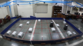
(a) $\phantom{0}5\times 10$ indoor workspace [cell size = $0.61$\mathrm{m}$$]

(b) $10\times 10$ outdoor workspace [cell size = $5$\mathrm{m}$$]

Figure 10: Workspaces for the real experiments

VI Conclusion

We have proposed a centralized online on-demand CPP algorithm that uses a goal assignment-based prioritized planning method at its core. Our CP guarantees complete coverage of an unknown workspace with multiple homogeneous failure-free robots. Experimental results demonstrate its superiority over its counterpart by decreasing the mission time significantly in large workspaces with hundreds of robots. In the future, we will extend our work to an approach dealing with simultaneous path planning and plan execution.

References

- [1] R. Bormann, F. Jordan, J. Hampp, and M. Hägele, “Indoor coverage path planning: Survey, implementation, analysis,” in ICRA, 2018, pp. 1718–1725.
- [2] I. Vandermeulen, R. Groß, and A. Kolling, “Turn-minimizing multirobot coverage,” in ICRA, 2019, pp. 1014–1020.
- [3] W. Jing, J. Polden, C. F. Goh, M. Rajaraman, W. Lin, and K. Shimada, “Sampling-based coverage motion planning for industrial inspection application with redundant robotic system,” in IROS, 2017, pp. 5211–5218.
- [4] D. Engelsons, M. Tiger, and F. Heintz, “Coverage path planning in large-scale multi-floor urban environments with applications to autonomous road sweeping,” in ICRA, 2022, pp. 3328–3334.
- [5] R. Schirmer, P. Biber, and C. Stachniss, “Efficient path planning in belief space for safe navigation,” in IROS, 2017, pp. 2857–2863.
- [6] A. Barrientos, J. Colorado, J. del Cerro, A. Martinez, C. Rossi, D. Sanz, and J. Valente, “Aerial remote sensing in agriculture: A practical approach to area coverage and path planning for fleets of mini aerial robots,” J. Field Robotics, vol. 28, no. 5, pp. 667–689, 2011.
- [7] W. Luo, C. Nam, G. Kantor, and K. P. Sycara, “Distributed environmental modeling and adaptive sampling for multi-robot sensor coverage,” in AAMAS, 2019, pp. 1488–1496.
- [8] N. Karapetyan, J. Moulton, J. S. Lewis, A. Q. Li, J. M. O’Kane, and I. M. Rekleitis, “Multi-robot dubins coverage with autonomous surface vehicles,” in ICRA, 2018, pp. 2373–2379.
- [9] S. Agarwal and S. Akella, “Line coverage with multiple robots,” in ICRA, 2020, pp. 3248–3254.
- [10] J. S. Lewis, W. Edwards, K. Benson, I. M. Rekleitis, and J. M. O’Kane, “Semi-boustrophedon coverage with a dubins vehicle,” in IROS, 2017, pp. 5630–5637.
- [11] T. M. Cabreira, L. B. Brisolara, and P. R. Ferreira Jr, “Survey on coverage path planning with unmanned aerial vehicles,” Drones, vol. 3, no. 1, p. 4, 2019.
- [12] S. Dogru and L. Marques, “Improved coverage path planning using a virtual sensor footprint: a case study on demining,” in ICRA, 2019, pp. 4410–4415.
- [13] Y. Bouzid, Y. Bestaoui, and H. Siguerdidjane, “Quadrotor-uav optimal coverage path planning in cluttered environment with a limited onboard energy,” in IROS, 2017, pp. 979–984.
- [14] A. Kleiner, R. Baravalle, A. Kolling, P. Pilotti, and M. Munich, “A solution to room-by-room coverage for autonomous cleaning robots,” in IROS, 2017, pp. 5346–5352.
- [15] G. Sharma, A. Dutta, and J. Kim, “Optimal online coverage path planning with energy constraints,” in AAMAS, 2019, pp. 1189–1197.
- [16] M. Wei and V. Isler, “Coverage path planning under the energy constraint,” in ICRA, 2018, pp. 368–373.
- [17] M. Coombes, W. Chen, and C. Liu, “Flight testing boustrophedon coverage path planning for fixed wing uavs in wind,” in ICRA, 2019, pp. 711–717.
- [18] X. Chen, T. M. Tucker, T. R. Kurfess, and R. W. Vuduc, “Adaptive deep path: Efficient coverage of a known environment under various configurations,” in IROS, 2019, pp. 3549–3556.
- [19] M. Dharmadhikari, T. Dang, L. Solanka, J. Loje, H. Nguyen, N. Khedekar, and K. Alexis, “Motion primitives-based path planning for fast and agile exploration using aerial robots,” in ICRA, 2020, pp. 179–185.
- [20] L. Zhu, S. Yao, B. Li, A. Song, Y. Jia, and J. Mitani, “A geometric folding pattern for robot coverage path planning,” in ICRA, 2021, pp. 8509–8515.
- [21] E. Galceran and M. Carreras, “A survey on coverage path planning for robotics,” Robotics Auton. Syst., vol. 61, no. 12, pp. 1258–1276, 2013.
- [22] J. Modares, F. Ghanei, N. Mastronarde, and K. Dantu, “UB-ANC planner: Energy efficient coverage path planning with multiple drones,” in ICRA, 2017, pp. 6182–6189.
- [23] N. Karapetyan, K. Benson, C. McKinney, P. Taslakian, and I. M. Rekleitis, “Efficient multi-robot coverage of a known environment,” in IROS, 2017, pp. 1846–1852.
- [24] M. Salaris, A. Riva, and F. Amigoni, “Multirobot coverage of modular environments,” in AAMAS, 2020, pp. 1178–1186.
- [25] G. Hardouin, J. Moras, F. Morbidi, J. Marzat, and E. M. Mouaddib, “Next-best-view planning for surface reconstruction of large-scale 3D environments with multiple uavs,” in IROS, 2020, pp. 1567–1574.
- [26] J. Tang, C. Sun, and X. Zhang, “Mstc: Multi-robot coverage path planning under physical constrain,” in ICRA, 2021, pp. 2518–2524.
- [27] L. Collins, P. Ghassemi, E. T. Esfahani, D. S. Doermann, K. Dantu, and S. Chowdhury, “Scalable coverage path planning of multi-robot teams for monitoring non-convex areas,” in ICRA, 2021, pp. 7393–7399.
- [28] N. Hazon and G. A. Kaminka, “Redundancy, efficiency and robustness in multi-robot coverage,” in ICRA, 2005, pp. 735–741.
- [29] X. Zheng, S. Jain, S. Koenig, and D. Kempe, “Multi-robot forest coverage,” in IROS, 2005, pp. 3852–3857.
- [30] A. Riva and F. Amigoni, “A GRASP metaheuristic for the coverage of grid environments with limited-footprint tools,” in AAMAS, 2017, pp. 484–491.
- [31] C. Cao, J. Zhang, M. J. Travers, and H. Choset, “Hierarchical coverage path planning in complex 3d environments,” in ICRA, 2020, pp. 3206–3212.
- [32] R. K. Ramachandran, L. Zhou, J. A. Preiss, and G. S. Sukhatme, “Resilient coverage: Exploring the local-to-global trade-off,” in IROS, 2020, pp. 11 740–11 747.
- [33] H. Song, J. Yu, J. Qiu, Z. Sun, K. Lang, Q. Luo, Y. Shen, and Y. Wang, “Multi-uav disaster environment coverage planning with limited-endurance,” in ICRA, 2022, pp. 10 760–10 766.
- [34] B. Yamauchi, “Frontier-based exploration using multiple robots,” in AGENTS, K. P. Sycara and M. J. Wooldridge, Eds., 1998, pp. 47–53.
- [35] A. Howard, L. E. Parker, and G. S. Sukhatme, “Experiments with a large heterogeneous mobile robot team: Exploration, mapping, deployment and detection,” Int. J. Robotics Res., vol. 25, no. 5-6, pp. 431–447, 2006.
- [36] A. Bircher, M. Kamel, K. Alexis, H. Oleynikova, and R. Siegwart, “Receding horizon “next-best-view” planner for 3D exploration,” in ICRA, 2016, pp. 1462–1468.
- [37] A. Mannucci, S. Nardi, and L. Pallottino, “Autonomous 3D exploration of large areas: A cooperative frontier-based approach,” in MESAS, vol. 10756. Springer, 2017, pp. 18–39.
- [38] E. A. Jensen and M. L. Gini, “Online multi-robot coverage: Algorithm comparisons,” in AAMAS, 2018, pp. 1974–1976.
- [39] S. N. Das and I. Saha, “Rhocop: receding horizon multi-robot coverage,” in ICCPS, 2018, pp. 174–185.
- [40] A. Özdemir, M. Gauci, A. Kolling, M. D. Hall, and R. Groß, “Spatial coverage without computation,” in ICRA, 2019, pp. 9674–9680.
- [41] S. Datta and S. Akella, “Prioritized indoor exploration with a dynamic deadline,” in IROS, 2021, pp. 3131–3137.
- [42] Y. Gabriely and E. Rimon, “Spanning-tree based coverage of continuous areas by a mobile robot,” in ICRA, 2001, pp. 1927–1933.
- [43] M. Li, A. Richards, and M. Sooriyabandara, “Asynchronous reliability-aware multi-uav coverage path planning,” in ICRA, 2021, pp. 10 023–10 029.
- [44] R. Mitra and I. Saha, “Scalable online coverage path planning for multi-robot systems,” in IROS, 2022, pp. 10 102–10 109.
- [45] Z. J. Butler, A. A. Rizzi, and R. L. Hollis, “Complete distributed coverage of rectilinear environments,” in Algorithmic and Computational Robotics. AK Peters/CRC Press, 2001, pp. 61–68.
- [46] N. Hazon, F. Mieli, and G. A. Kaminka, “Towards robust on-line multi-robot coverage,” in ICRA, 2006, pp. 1710–1715.
- [47] I. M. Rekleitis, A. P. New, E. S. Rankin, and H. Choset, “Efficient boustrophedon multi-robot coverage: an algorithmic approach,” Ann. Math. Artif. Intell., vol. 52, no. 2-4, pp. 109–142, 2008.
- [48] E. A. Jensen and M. L. Gini, “Rolling dispersion for robot teams,” in IJCAI, 2013, pp. 2473–2479.
- [49] K. Hungerford, P. Dasgupta, and K. R. Guruprasad, “A repartitioning algorithm to guarantee complete, non-overlapping planar coverage with multiple robots,” in DARS, N. Y. Chong and Y. Cho, Eds., vol. 112, 2014, pp. 33–48.
- [50] H. H. Viet, V. Dang, S. Y. Choi, and T. Chung, “BoB: an online coverage approach for multi-robot systems,” Appl. Intell., vol. 42, no. 2, pp. 157–173, 2015.
- [51] L. Siligardi, J. Panerati, M. Kaufmann, M. Minelli, C. Ghedini, G. Beltrame, and L. Sabattini, “Robust area coverage with connectivity maintenance,” in ICRA, 2019, pp. 2202–2208.
- [52] J. Song and S. Gupta, “CARE: cooperative autonomy for resilience and efficiency of robot teams for complete coverage of unknown environments under robot failures,” Auton. Robots, vol. 44, no. 3-4, pp. 647–671, 2020.
- [53] M. Hassan, D. Mustafic, and D. Liu, “Dec-ppcpp: A decentralized predator-prey-based approach to adaptive coverage path planning amid moving obstacles,” in IROS, 2020, pp. 11 732–11 739.
- [54] TurtleBot. [Online]. Available: https://www.turtlebot.com/
- [55] TurtleBot 2. [Online]. Available: https://clearpathrobotics.com/turtlebot-2-open-source-robot/
- [56] P. Oberlin, S. Rathinam, and S. Darbha, “A transformation for a heterogeneous, multiple depot, multiple traveling salesman problem,” in ACC, 2009, pp. 1292–1297.
- [57] S. M. LaValle, Planning Algorithms. Cambridge University Press, 2006.
- [58] S. J. Russell and P. Norvig, Artificial Intelligence - A Modern Approach, Third International Edition. Pearson Education, 2010.
- [59] H. W. Kuhn, “The hungarian method for the assignment problem,” Nav. Res. Logist., vol. 2, no. 1-2, pp. 83–97, 1955.
- [60] F. Bourgeois and J. Lassalle, “An extension of the munkres algorithm for the assignment problem to rectangular matrices,” Commun. ACM, vol. 14, no. 12, pp. 802–804, 1971.
- [61] M. A. Erdmann and T. Lozano-Pérez, “On multiple moving objects,” in ICRA, 1986, pp. 1419–1424.
- [62] D. Silver, “Cooperative pathfinding,” in AIIDE, 2005, pp. 117–122.
- [63] J. P. van den Berg and M. H. Overmars, “Prioritized motion planning for multiple robots,” in IROS, 2005, pp. 430–435.
- [64] M. Turpin, K. Mohta, N. Michael, and V. Kumar, “Goal assignment and trajectory planning for large teams of aerial robots,” in RSS, 2013.
- [65] R. Hassin and S. Rubinstein, “Approximations for the maximum acyclic subgraph problem,” Inf. Process. Lett., vol. 51, no. 3, pp. 133–140, 1994.
- [66] S. Skiena, The Algorithm Design Manual, Second Edition. Springer, 2008.
- [67] Robot Operating System. [Online]. Available: https://www.ros.org/
- [68] R. Stern, N. R. Sturtevant, A. Felner, S. Koenig, H. Ma, T. T. Walker, J. Li, D. Atzmon, L. Cohen, T. K. S. Kumar, R. Barták, and E. Boyarski, “Multi-agent pathfinding: Definitions, variants, and benchmarks,” in SOCS, 2019, pp. 151–159.
- [69] R. Mitra and I. Saha, “Online on-demand multi-robot coverage path planning,” CoRR, vol. abs/2303.00047, 2023. [Online]. Available: https://arxiv.org/abs/2303.00047
- [70] DJI Consumer Drones Comparison. [Online]. Available: https://www.dji.com/global/products/comparison-consumer-drones
- [71] N. P. Koenig and A. Howard, “Design and use paradigms for gazebo, an open-source multi-robot simulator,” in IROS, 2004, pp. 2149–2154.
- [72] Vicon Motion Capture Systems. [Online]. Available: https://www.vicon.com/