A Redundancy Resolution Method for Free-Floating Underwater Manipulation

Abstract

Underwater manipulation with free-floating autonomous underwater vehicles (AUVs) is an under-explored research area that this paper addresses. The open-source mechanical, electrical, and software designs of an AUV and continuum manipulator system are provided as a platform for performing this research. The underwater robot system has high degrees of freedom including the vehicle body motion and the manipulator joints. Therefore, when performing a manipulation task, the robot has many different potential trajectories which satisfy the task constraints, and this kinematic redundancy needs to be resolved. This paper provides a method for solving the redundancy problem. The relevant kinematic models are derived in order to build an algorithm to calculate desired joint velocities in real time. Different methods to optimize the algorithm for specific tasks are proposed, including a basic weighting method and a gradient projection method to optimize a user-defined objective function. Both simulation and experimental results are analyzed to assess the performance of this algorithm.

I Introduction

Underwater robotics is a growing field with practical applications including exploration [1], inspection [2], and aquaculture [3]. Traditionally, underwater robotics has relied on teleoperation of remotely operated vehicles (ROVs), but recent work has focused on autonomous underwater vehicles (AUVs). One of the biggest difficulties comes from the problem of localization and navigation for AUVs, as summarized in [4]. This has led to advancements in simultaneous localization and mapping (SLAM) and even 3D reconstruction of the environment using acoustic or optical methods in works such as [5, 6, 7, 8, 9, 10, 11].

An under-explored topic within underwater robotics is free-floating manipulation, in which a manipulator is attached to an AUV platform to perform intervention tasks. Autonomous underwater manipulation is a very challenging problem due to the aforementioned state estimation difficulties and has been the focus of recent work [12, 13, 14, 15, 16, 17, 18, 19, 20]. The robots used for field experiments are often very large and expensive, creating additional barriers to research in this field. However, smaller low-cost AUVs are deployed in works such as [8, 9, 10].

Commercially available underwater arms for use on smaller AUVs are listed in [14]; however, these designs are large and heavy rigid-link manipulators, with weights ranging from 10 kg to over 50 kg. Many of these are powered via hydraulic systems, although electric-powered arms are also available. Fewer examples of continuum manipulators for underwater manipulation exist, and most are limited in scope to seabed applications, such as seafloor locomotion in [21] and [22] as well as delicate grasping in shallow water in [23]. In our previous work, we developed a compact, low cost, and easy to fabricate underwater continuum manipulator [24], but integration with the AUV is addressed in this paper.

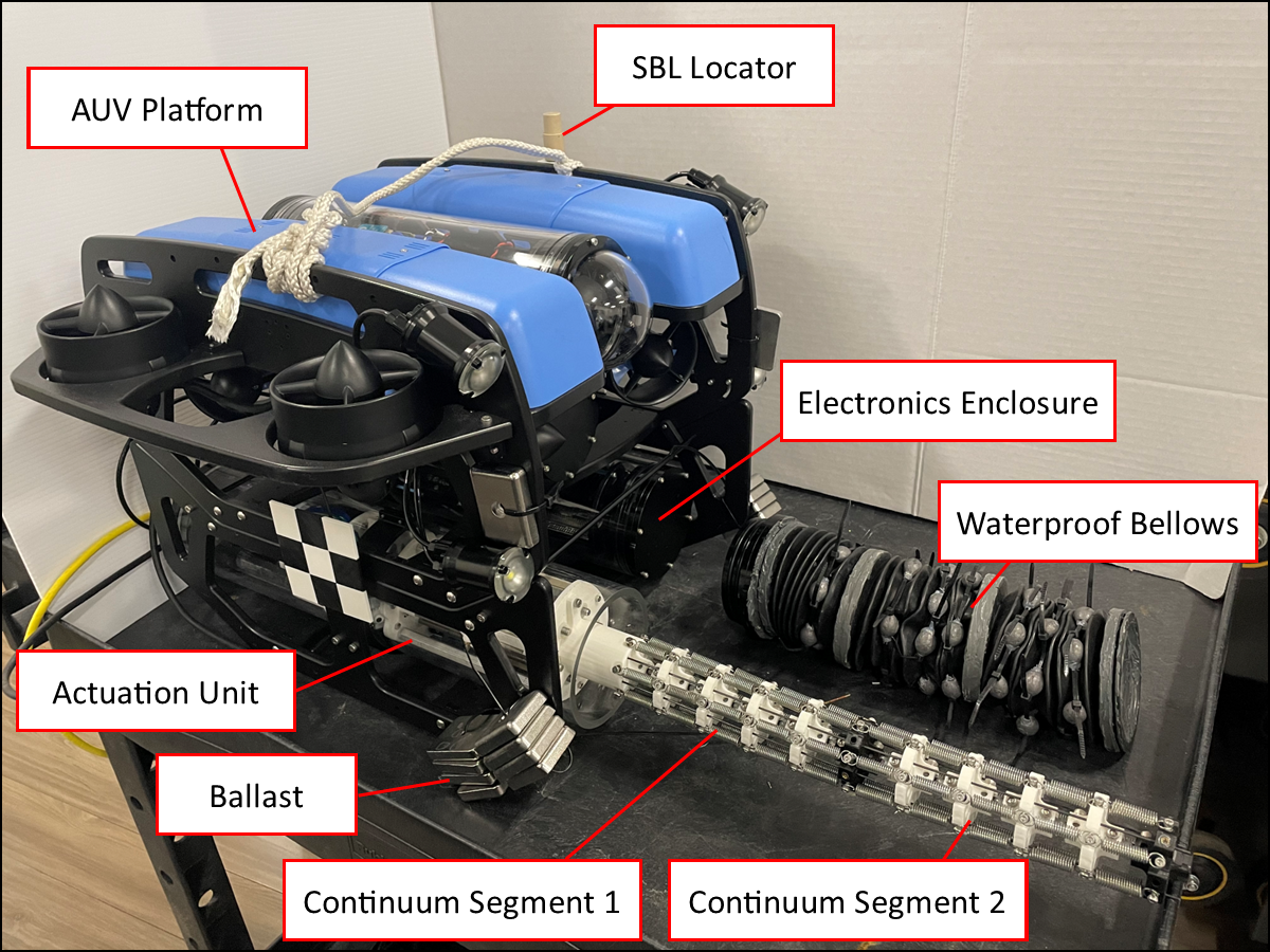
Figure 1: AUV and continuum arm integration

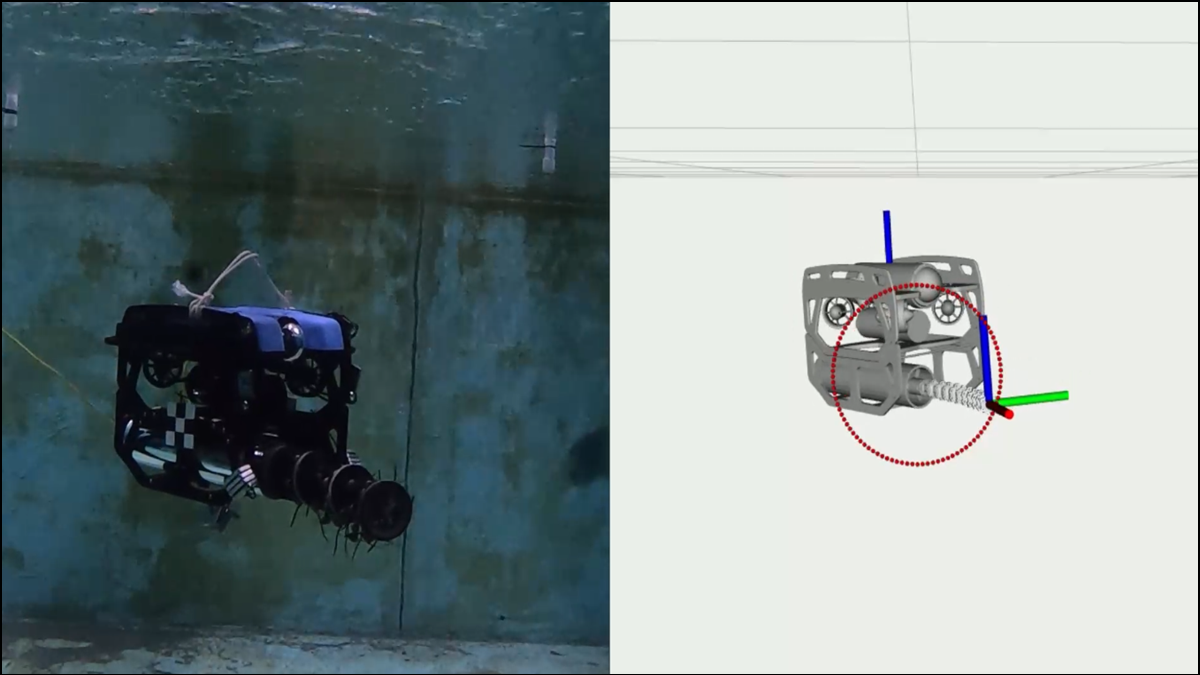
Figure 2: Side-by-side comparison of actual (left) and measured (right) pose of AUV and manipulator.

In this paper, the problem of redundancy resolution for free-floating manipulation is addressed. When a mobile AUV is integrated with a manipulator with multiple degrees of freedom (DoFs), the resulting system will typically have more DoFs than is required to satisfy task constraints such as reaching a specific end effector position and orientation. The redundancy leads to an infinite number of ways the robot can satisfy a given task from its initial configuration. Kinematic redundancy of fixed base [25] or wheeled mobile manipulators [26] has been explored in previous works, but to our knowledge, kinematic redundancy in free-floating mobile robots has not been explored. Our work attempts to exploit the available redundancy to find an optimal trajectory for the manipulator-equipped AUV. We demonstrate our algorithm on a specific platform integrated with a continuum manipulator. We also provide the open-source designs and software in [27].

This paper is outlined as follows. Section II describes the derivation of the differential kinematics for the robotic system, implementation of the redundancy resolution algorithm, and how the algorithm can be optimized with respect to additional tasks while satisfying the primary task. In Section III, we validate the algorithm in simulation to demonstrate the effects of optimization on the planned trajectory. Section IV discusses the mechanical design of the continuum arm and how it is integrated with the AUV platform. In Section V, the continuum arm and AUV are combined in an underwater experiment to demonstrate the validity of the redundancy resolution algorithm. Finally, Section VI discusses the results of the experiments and how the methods introduced can be further adapted for practical applications.

II Kinematics and Redundancy Resolution

A free-floating robot will naturally have more DoFs than a grounded robot due to the additional axis of movement and possibility of orientation changes across three axes instead of just one. For many applications, the robot will also have a manipulator to allow it to interact with its environment and complete tasks such as operating a tool or perching onto a structure. In such a task, the robot end effector must achieve a specific pose (position and orientation), which will typically require the system to have six DoFs. However, a free-floating robot with a manipulator will likely have more DoFs than this, which is known as kinematic redundancy.

A kinematically redundant robot will have an infinite number of ways to achieve its task, which requires more planning and decision-making. However, it also allows the robot to consider other objectives to complete additional subtasks. This section will discuss an algorithm to resolve a free-floating robot’s redundancy using kinematics. This algorithm generates a locally optimal trajectory based on an arbitrary objective function and publishes the AUV and manipulator commands in real time via ROS. The basis for this method is adapted from works such as [28, 29, 30, 31].

The free-floating robot system considered in this paper is comprised of an AUV and a continuum manipulator. The use of a continuum manipulator instead of a traditional rigid-link manipulator adds compliance and flexibility to the system, which can be useful as a softer contact between the robot and its environment or to allow the manipulator to operate inside a pipe or other confined spaces. However, much of the methodology presented in this paper could apply just as well to a traditional manipulator with multiple DoFs.

II-A Jacobian Derivation

The total Jacobian matrix relates the linear and angular velocities of the end effector in the global coordinate system (GCS) to the AUV and continuum manipulator state velocities. In this section, we derive the Jacobian matrices for the manipulator and then integrate them with the AUV Jacobian matrix to form the total Jacobian matrix.

As reported in our prior work [24], kinematics for continuum manipulators includes mappings between three spaces: task space, configuration space, and joint space. In addition, for a single-segment continuum manipulator, two Jacobian matrices for configuration-to-task space and for configuration-to-joint space, respectively, were given in [24]. In this paper, the configuration-to-task space Jacobian will be used to form the manipulator Jacobian matrix as below, and the configuration-to-joint space Jacobian will be used in low-level control only.

As mentioned in Section IV-A, the continuum arm used in this paper has been modified by adding a second segment, increasing the degrees of freedom of the continuum arm to four. This allows for greater dexterity in the manipulator and redundancy in the whole system.

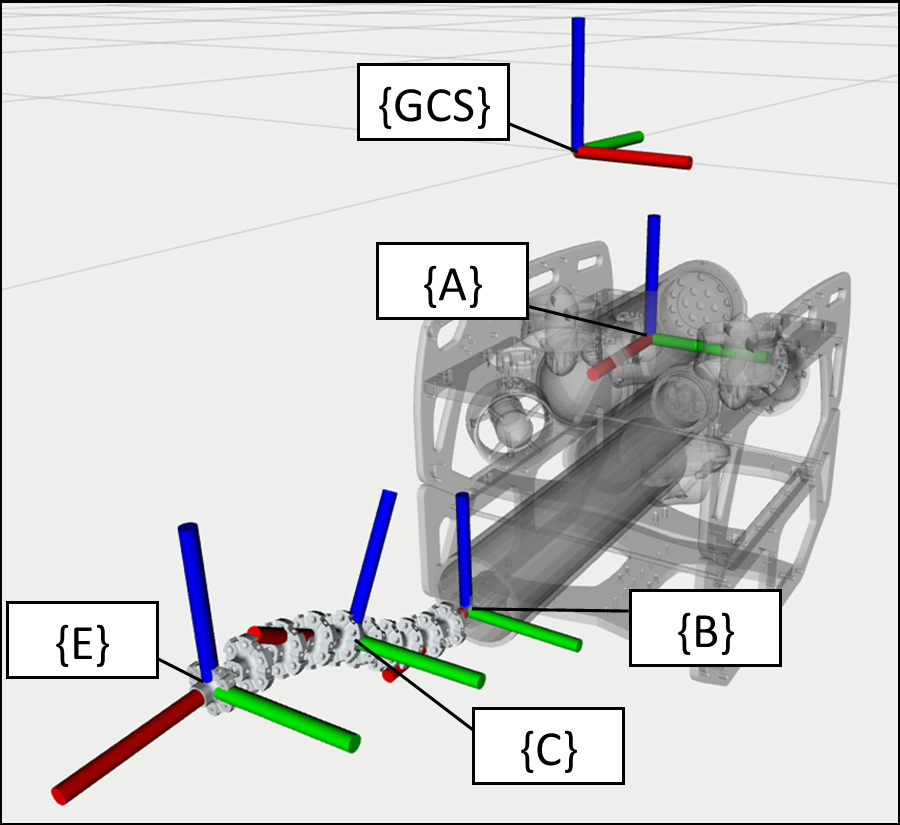
Figure 3: AUV system coordinate frames. {GCS} - global coordinate system; {A} - the moving base of AUV; {B} - the base of $1^{\text{st}}$ continuum segment; {C} - the base of $2^{\text{nd}}$ continuum segment; {E} - end effector.

To represent the full state of the AUV and continuum manipulator, the total Jacobian needs to also account for the six additional DoFs from the mobile AUV platform, which represent its position and orientation in 3D space. The total state of the robot is represented by the vector $\boldsymbol{\Psi}$:

$$\boldsymbol{\Psi}=\begin{bmatrix}x&y&z&\alpha&\beta&\gamma&\theta_{1}&\phi_{1}&\theta_{2}&\phi_{2}\end{bmatrix}^{\mathrm{T}}$$ (1)

$$\boldsymbol{\Psi}\in\hbox{I \kern-2.5ptR}^{10}$$ (2)

The vector $\boldsymbol{\Psi}$ includes vehicle states and manipulator configuration states. Variables $x$, $y$, and $z$ represent the linear position of the AUV, with $\mathbf{p}_{\text{AUV}}=\begin{bmatrix}x&y&z\end{bmatrix}^{\mathrm{T}}$. Variables $\alpha$, $\beta$, and $\gamma$ represent respectively the yaw, pitch, and roll angles of the AUV attitude, which can be represented in rotation matrix form as $\mathbf{R}_{\text{a}}$. Variables $\theta_{i}$ and $\phi_{i}$ represent respectively the bending angle and the bending plane direction angle for the $i^{\text{th}}$ continuum segment. The pose of the end effector relative to frame $\{GCS\}$ is defined as:

$$\mathbf{x}=\begin{bmatrix}\mathbf{p}^{\mathrm{T}}&\boldsymbol{\mu}^{\mathrm{T}}\end{bmatrix}^{\mathrm{T}}$$ (3)

$$\mathbf{p}=\mathbf{p}_{\text{AUV}}+\mathbf{R}_{a}\;^{a}\mathbf{r}_{\text{base}}+\mathbf{R}_{b}\;^{b}\mathbf{r}_{\text{EE}_{1}}+\mathbf{R}_{c}\;^{c}\mathbf{r}_{\text{EE}_{2}}$$ (4)

where $\mathbf{p}$ and $\boldsymbol{\mu}$ are $3\times 1$ vectors that represent the end effector position and orientation in rotation vector format relative to frame $\{GCS\}$, ${}^{a}\mathbf{r}_{\text{base}}$ represents the position of the base of continuum segment 1 relative to frame $\{A\}$, ${}^{b}\mathbf{r}_{\text{EE}_{1}}$ represents the end position of continuum segment 1 relative to frame $\{B\}$, and ${}^{c}\mathbf{r}_{\text{EE}_{2}}$ represents the end position of continuum segment 2 relative to frame $\{C\}$. Each rotation matrix corresponds to the orientation of the same frame as shown in Fig. 3.

We then will start deriving the total Jacobian matrix:

$$\dot{\mathbf{x}}=\mathbf{J}\;\dot{\boldsymbol{\Psi}},\quad\mathbf{J}\in\hbox{I \kern-2.5ptR}^{6\times 10}$$ (5)

First, we consider the configuration-to-task space Jacobian matrix $\mathbf{J}_{c,i}$ for the $i^{\text{th}}$ continuum segment:

$$\mathbf{J}_{c,i}=\begin{bmatrix}\mathbf{J}_{p,i}\\ \mathbf{J}_{\mu,i}\end{bmatrix}$$ (6)

$$\mathbf{J}_{c,i}\in\hbox{I \kern-2.5ptR}^{6\times 2},\;\mathbf{J}_{p,i}\in\hbox{I \kern-2.5ptR}^{3\times 2},\;\mathbf{J}_{\mu,i}\in\hbox{I \kern-2.5ptR}^{3\times 2}$$ (7)

Derivation of the position and orientation Jacobians, $\mathbf{J}_{p,i}$ and $\mathbf{J}_{\mu,i}$, as well as the continuum segment displacements, ${}^{b}\mathbf{r}_{\text{EE}_{1}}$ and ${}^{c}\mathbf{r}_{\text{EE}_{2}}$, can be found in [24]. The transformation of these Jacobians into the GCS leads to the total Jacobian matrix:

$$\mathbf{J}=\begin{bmatrix}\boldsymbol{\Gamma}_{1}&\boldsymbol{\Gamma}_{2}&\boldsymbol{\Gamma}_{3}\end{bmatrix}$$ (8)

where

$$\boldsymbol{\Gamma}_{1}=\left[\begin{array}[]{c;{2pt/2pt}c}\underbrace{\raisebox{-14.22636pt}{\phantom{}}\begin{bmatrix}\mathbf{I}_{3\times 3}\\ \mathbf{0}\end{bmatrix}}_{\text{AUV Linear Position}}&\underbrace{\begin{bmatrix}\left[\left({}^{a}\mathbf{r}_{b}\right)^{\wedge}\right]^{\mathrm{T}}\\ \mathbf{I}_{3 \times 3}\end{bmatrix} \mathbf{T}}_\text{AUV Angular Position}\end{array}\right]$$ (10)

$$\boldsymbol{\Gamma}_{2}=\underbrace{\raisebox{-14.22636pt}{\phantom{}}\left[\begin{bmatrix}\mathbf{R}_{a}&\left[\left({}^{a}\mathbf{r}_{b}\right)^{\wedge}\right]^{\mathrm{T}}\;\mathbf{R}_{a}\\ \mathbf{0}&\mathbf{R}_{a}\end{bmatrix}\;\mathbf{J}_{c,1}\right]}_{1^{\text{st}}\text{ Continuum Segment}}$$ (11)

$$\boldsymbol{\Gamma}_{3}=\underbrace{\raisebox{-14.22636pt}{\phantom{}}\left[\begin{bmatrix}\mathbf{R}_{c}&\mathbf{0}\\ \mathbf{0}&\mathbf{R}_{c}\end{bmatrix}\;\mathbf{J}_{c,2}\right]}_{2^{\text{nd}}\text{ Continuum Segment}}$$ (12)

where $\left[(\cdot)^{\wedge}\right]$ represents the skew-symmetric matrix operator. Matrix $\mathbf{T}$ represents the relation between Euler-angle rates and body-axis rates and is given by:

$$\mathbf{T}=\begin{bmatrix}0&\quad-\sin{\alpha}&\quad\cos{\alpha}\;\cos{\beta}\\ 0&\quad\cos{\alpha}&\quad\sin{\alpha}\;\cos{\beta}\\ 1&\quad 0&\quad-\sin{\beta}\end{bmatrix}$$ (14)

Worth noting is that this model presumes the AUV has six degree of freedom control; however, some AUVs only provide four degrees of freedom control (position and yaw). In this case, $\beta$ and $\gamma$ can be removed from $\boldsymbol{\Psi}$, and the corresponding columns (the $5^{\text{th}}$ and $6^{\text{th}}$) are removed from the total Jacobian matrix $\mathbf{J}$.

II-B Redundancy Resolution Algorithm

We start by considering the simple case of the weighted minimum norm problem described as below:

$$\begin{array}[]{cc}\text{min. }&\frac{1}{2}\;\left(\dot{\boldsymbol{\Psi}}^{\mathrm{T}}\;\mathbf{W}\;\dot{\boldsymbol{\Psi}}\right)\\ \text{subject to: }&\dot{\mathbf{x}}=\mathbf{J}\;\dot{\boldsymbol{\Psi}}\end{array}$$ (15)

where $\dot{\mathbf{x}}$ is the desired end-effector twist. The choice of the weighting matrix $\mathbf{W}$ is discussed in more detail in Section II-C. In this case, we will assume the AUV has position and yaw control, which means $\boldsymbol{\Psi}\in\hbox{I \kern-2.5ptR}^{8}$ and $\mathbf{J}\in\hbox{I \kern-2.5ptR}^{6\times 8}$. The weighted minimum norm solution to this problem is given by:

$$\dot{\boldsymbol{\Psi}}=\mathbf{W}^{-1}\;\mathbf{J}^{\mathrm{T}}\left(\mathbf{J}\;\mathbf{W}^{-1}\;\mathbf{J}^{\mathrm{T}}\right)^{-1}\dot{\mathbf{x}}$$ (16)

This solution gives the state velocities that satisfy a desired end effector twist $\dot{\mathbf{x}}$ while minimizing the weighted norm of the state velocity vector $\dot{\boldsymbol{\Psi}}$. The desired end effector twist, $\dot{\mathbf{x}}$, must be properly chosen in order to achieve the desired pose. We implement a resolved rates algorithm to resolve in real time the desired linear and angular velocity magnitudes $v_{\text{mag}}$ and $\omega_{\text{mag}}$ until it reaches the goal.

The resolved rates has been implemented alongside the redundancy resolution formulation as described in this section as well as Algorithm 1. The desired linear velocity vector points from the current end effector position $\mathbf{p}$ to the desired position $\mathbf{p}_{d}$. As the end effector approaches the goal, the magnitude will decrease from a constant $v_{\text{max}}$ when it is far away to $v_{\text{min}}$ as a function of the error threshold $e_{p}$ as well as scaling parameter $\lambda_{p}$. The desired angular velocity vector is applied along vector $\mathbf{m}$ which is found using the axis angle representation of the orientation error matrix $\mathbf{R}_{\text{err}}$. Like the desired linear velocity, the desired angular velocity decreases in magnitude from $\omega_{\text{max}}$ to $\omega_{\text{min}}$ as a function of the error threshold $e_{\mu}$ and scaling parameter $\lambda_{\mu}$.

After the end effector twist has been calculated, the Jacobian and weighting matrices are updated to reflect the current robot state $\boldsymbol{\Psi}$. The desired robot state velocities $\dot{\boldsymbol{\Psi}}$ are calculated using (16). Then, the commanded robot state is updated for the next time step and published to ROS according to Fig. 7. The end effector is considered to have reached the desired pose when the position and orientation errors are within these error thresholds, terminating the algorithm in the case of a fixed goal or continuing in the case of a moving trajectory.

Algorithm 1 Redundancy Resolution with Resolved Rates

Initialize: $\quad\mathbf{x},\leftarrow\mathbf{x}_{0}$, $\quad\Psi\leftarrow\Psi_{0}$

Goal Pose: $\quad\mathbf{x}_{d}\leftarrow\begin{bmatrix}\mathbf{p}_{d}^{\mathrm{T}}&\boldsymbol{\mu}_{d}^{\mathrm{T}}\end{bmatrix}^{\mathrm{T}}$

Objective Function: $\quad g(\mathbf{\boldsymbol{\Psi}})$

while $\delta_{p}>e_{p}\;||\;\delta_{\mu}>e_{\mu}$ do

    Step 1 - Get current pose:

$$\mathbf{p},\;\mathbf{R}\leftarrow\text{Kinematic Model}$$

    Step 2 - Compute errors:

$$\delta_{p}=\sqrt{(\mathbf{p}_{d}-\mathbf{p})^{\mathrm{T}}\;(\mathbf{p}_{d}-\mathbf{p})}$$ (17)

$$\mathbf{R}_{\text{err}}=\mathbf{R}_{d}\;\mathbf{R}^{\mathrm{T}},\quad\mu_{\text{err}}=\arccos{\frac{\text{Tr}(\mathbf{R}_{\text{err}})-1}{2}}$$ (18)

$$\mathbf{m}=\frac{1}{2\;\sin{\mu_{\text{err}}}}\begin{bmatrix}\mathbf{R}_{\text{err}}^{32}-\mathbf{R}_{\text{err}}^{23}\\ \mathbf{R}_{\text{err}}^{13}-\mathbf{R}_{\text{err}}^{31}\\ \mathbf{R}_{\text{err}}^{21}-\mathbf{R}_{\text{err}}^{12}\end{bmatrix}$$ (19)

$$\delta_{\mu}=\sqrt{(\mu_{\text{err}}\;\mathbf{m})^{\mathrm{T}}\;(\mu_{\text{err}}\;\mathbf{m})}$$ (20)

    Step 3 - Compute desired end effector twist:

    if $\delta_{p}/e_{p}>\lambda_{p}$ then

$$v_{\text{mag}}=v_{\text{max}}$$

    else

$$v_{\text{mag}}=v_{\text{min}}+\frac{(v_{\text{max}}-v_{\text{min}})\;(\delta_{p}-e_{p})}{e_{p}\;(\lambda_{p}-1)}$$ (21)

    end if

    if $\delta_{\mu}/e_{\mu}>\lambda_{\mu}$ then

$$\omega_{\text{mag}}=\omega_{\text{max}}$$

    else

$$\omega_{\text{mag}}=\omega_{\text{min}}+\frac{(\omega_{\text{max}}-\omega_{\text{min}})\;(\delta_{\mu}-e_{\mu})}{e_{\mu}\;(\lambda_{\mu}-1)}$$ (22)

    end if

$$\text{Desired linear velocities:}\qquad\dot{\mathbf{p}}=v_{\text{mag}}\;\frac{\mathbf{p}_{d}-\mathbf{p}}{\delta_{p}}$$

$$\text{Desired angular velocities:}\qquad\dot{\boldsymbol{\mu}}=\omega_{\text{mag}}\;\mathbf{m}$$

$$\text{Desired twist:}\qquad\dot{\mathbf{x}}=\begin{bmatrix}\dot{\mathbf{p}}&\quad&\dot{\boldsymbol{\mu}}\end{bmatrix}^{\mathrm{T}}$$

    Step 4 - Compute redundancy resolution:

$$\mathbf{J},\mathbf{W}\leftarrow\boldsymbol{\Psi}$$ (23)

$$\begin{matrix}\dot{\boldsymbol{\Psi}}=&\mathbf{W}^{-1}\;\mathbf{J}^{\mathrm{T}}\;\left(\mathbf{J}\;\mathbf{W}^{-1}\;\mathbf{J}^{\mathrm{T}}\right)^{-1}\;\dot{\mathbf{x}}\phantom{xxspace}\\[6.0pt] &\lx@algorithmicx@hfill+\quad\left(\mathbf{I}-\mathbf{J}^{+}\;\mathbf{J}\right)\;k\;\nabla g\end{matrix}$$ (24)

$$\boldsymbol{\Psi}=\boldsymbol{\Psi}+\dot{\boldsymbol{\Psi}}\;\textrm{d}t$$ (25)

end while

II-C Task Optimization

A weighted minimum norm solution has been proposed in works such as [28] to solve the redundancy problem. The diagonal weighting matrix $\mathbf{W}=\text{diag}\left(w_{j}\right)$ allows the motion of certain degrees of freedom of the robot to be prioritized or penalized. Higher value weights correspond to higher penalties on the respective degree of freedom. In addition, these weights can be updated in real time based on the robot state. A useful application of this is to avoid joint limits by increasing the weight to infinite as the joint approaches its limit. The free-floating robot should prioritize using the degrees of freedom corresponding to the manipulator ($\theta_{1}$, $\phi_{1}$, $\theta_{2}$, and $\phi_{2}$) if the robot is in close range with the target, as this is more energy-efficient considering the vehicle inertia and current disturbance. But the robot should also avoid magnitudes of $\theta_{i}$ larger than $\frac{\pi}{4}$ to prevent stalling the motors when close to the configuration space “joint limits”. Therefore, we use the following weights:

$$w_{1\mathrel{\mathop{\mathchar 58\relax}}4}=1000$$ (26)

$$w_{\phi_{i}}=0.01$$ (27)

$$w_{\theta_{i}}=\begin{cases}1+\mathinner{\!\left\lvert\frac{\pi^{2}\;\theta_{i}}{8(\frac{\pi}{4}-\theta_{i})^{2}(\theta_{i}+\frac{\pi}{4})^{2}}\right\rvert}&\text{if}\;\Delta\mathinner{\!\left\lvert\theta_{i}\right\rvert}\geq 0\\ 1&\text{if}\;\Delta\mathinner{\!\left\lvert\theta_{i}\right\rvert}<0\end{cases}$$ (28)

The kinematic redundancy allows additional optimization subtasks to be solved simultaneously. Works such as [29] and [30] formulate the gradient projection method to maximize an objective function $g(\boldsymbol{\Psi})$ by projecting its gradient into the null space of the Jacobian:

$$\dot{\boldsymbol{\Psi}}=\mathbf{J}^{+}\;\dot{\mathbf{x}}+(\mathbf{I}-\mathbf{J}^{+}\;\mathbf{J})\;k\;\nabla g(\boldsymbol{\Psi})$$ (29)

where $\mathbf{J}^{+}$ denotes the Moore–Penrose (pseudo) inverse of $\mathbf{J}$.

The function $g(\boldsymbol{\Psi})$ can be chosen as any desired function to minimize or maximize as a subtask. As an example, consider the task of tracing a known circle in 3D space using the free-floating AUV and manipulator proposed in this paper. The task constraint in this example includes orienting the end effector perpendicularly to the circle, making it a six DoF problem. A convenient choice of the objective function is to minimize the distance between the origin of the AUV and a preferred “anchor point” $\mathbf{p}_{\text{anchor}}$ which in this case is chosen to approximately center the AUV within the circle. Figure 4 labels relevant coordinate frames using RViz visualization software, with $\{GCS\}$ representing the global origin, $\{A\}$ representing the AUV pose, $\{E\}$ representing the end effector pose, and $\{G\}$ representing the goal position. The circle to be traced is shown in this figure as well. The optimization function in this case is given by:

$$g(\boldsymbol{\Psi})=||\mathbf{p}_{\text{AUV}}-\mathbf{p}_{\text{anchor}}||$$ (30)

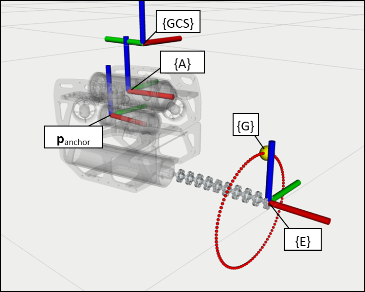
Figure 4: AUV simulation, with desired trajectory represented by the red circle. {G} - goal position; {Anchor} - anchor point

The scalar coefficient $k$ is chosen through trial and error in simulation, but more intelligent choice of this value has been explored in works such as [31]. The subtask-optimized resolved rates solution to the redundancy problem is therefore:

$$\begin{array}[]{ll}\dot{\boldsymbol{\Psi}}\quad=&\quad\underbrace{\mathbf{W}^{-1}\;\mathbf{J}^{\mathrm{T}}\left(\mathbf{J}\;\mathbf{W}^{-1}\;\mathbf{J}^{\mathrm{T}}\right)^{-1}\dot{\mathbf{x}}}_{\text{Task Constraint}}\\[24.0pt] &\hskip 56.9055pt+\qquad\underbrace{\left(\mathbf{I}-\mathbf{J}^{+}\;\mathbf{J}\right)\;k\;\nabla g(\boldsymbol{\Psi})}_{\text{Null Space Projection}}\end{array}$$ (31)

It’s worth noting that we replace the minimum norm solution part in (29) with the weighted minimum norm solution to keep the joint preferences intact. In a test case, the gradient $\nabla g$ is only dependent on the AUV position, so only the first three elements will be non-zero:

$$\nabla g(\boldsymbol{\Psi})=\frac{1}{\|\mathbf{p}_{\text{AUV}}-\mathbf{p}_{\text{anchor}}\|}\;\begin{bmatrix}\mathbf{p}_{\text{AUV}}-\mathbf{p}_{\text{anchor}}\\ \mathbf{0}_{5\times 1}\end{bmatrix}$$ (32)

III Simulation Validation

To validate the algorithm proposed to resolve the redundancy of the free-floating AUV system, a kinematic simulation of the end-effector following a circular trajectory was conducted under different conditions. The robot, desired trajectory, and goal point can all be seen in a series of frames displayed in Figure 5. This figure compares results of the circle tracing task using three different solutions proposed in Section II-C. The first solution utilizes Algorithm 1 without any weighting matrix or additional objective functions. The second solution implements a weighting matrix that prioritizes use of the manipulator’s degrees of freedom while simultaneously introducing joint limits on bending angles $\theta_{1}$ and $\theta_{2}$ according to (26) through (28). The third solution introduces the objective function in (30) corresponding to the optimized solution in (16).

Each solution in Figure 5 demonstrates high accuracy and smoothness in tracing the circle, showing that each is a valid solution that satisfies the task constraint. However, the first solution, illustrated in row (A) in Fig. 5, requires the AUV to do almost all of the work, following the goal with very small motion in the manipulator. This has many drawbacks in practical applications, including higher power consumption and lower precision. In contrast, the second solution, illustrated in row (B) of Fig. 5, utilizes the manipulator much more, allowing the AUV to trace the circle without much lateral motion. However, this still requires a decent amount of vertical displacement. The third solution, illustrated in row (C) of Fig. 5, allows the AUV to stay roughly within the center of the circle by better utilizing the manipulator and yaw motion. The AUV still needs to move around to satisfy the task constraint, but this solution strays the least from the preferred anchor point, which is represented by the coordinate frame behind the AUV in the figure.

These are three example solutions to this task, as there are many other ways to utilize the system’s redundancy to solve this task using equation (31). Careful choice of the objective function could allow for optimization with respect to energy consumption, manipulator stiffness, or minimization of free-floating vehicle pose uncertainty. Additional objectives could be simultaneously optimized using a task priority method [31, 30, 26] if desired.

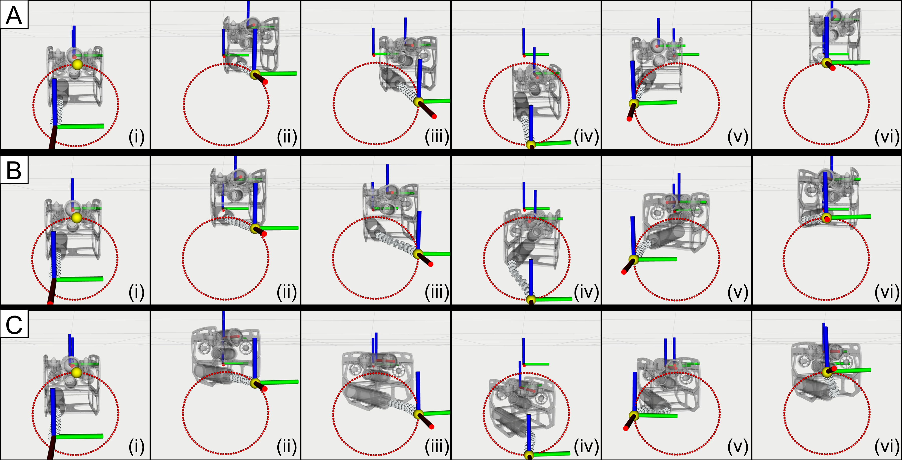
Figure 5: Simulated trajectory using (A): no weights or objective function; (B): weights without objective function; (C): both weights and objective function.

IV Experimental Robot Hardware

To test the feasibility of free-floating manipulation using the proposed algorithm, we developed experimental hardware as reported in this section.

IV-A Mechanical Design & Prototype Development

The continuum robot arm used in this paper is a two-segment multi-backbone design adapted from the previously developed design in [24]. The most significant change in the continuum arm design is the addition of a second continuum segment, giving the entire arm a total of four DoFs. This allows the distal portion of the arm to bend independently from the proximal portion, increasing its maneuverability and dexterity. The continuum manipulator is actuated via two sets of three nitinol wires which pull on the end link of each segment. The wires are connected to an actuation unit which creates the linear pulling motion via six lead screws and servo motors inside a waterproof enclosure. A flexible bellows with distributed ballast covers the continuum arm to make the whole system waterproof and neutrally buoyant.

The AUV platform used in this paper is the BlueROV2 by Blue Robotics, Inc. [32]. This platform was chosen because of its low cost and ease of integration via an additional payload skid, customizable waterproof enclosures and penetrators, and their Heavy Configuration upgrade to improve stability and maneuverability. The continuum arm and the electronics enclosure, described in more detail in Section IV-B, are mounted side-by-side on the payload skid underneath the body of the AUV. Figure 1 labels the components of the system on the robot, with the waterproof bellows removed for visibility.

IV-B Communications and Controls

Communication between the AUV and the continuum arm is achieved via a single shielded twisted pair waterproof tether. A schematic of the entire electronics system can be seen in Figure 6.

The deployed system is broken up into three waterproof enclosures. The actuation unit contains the microprocessors, sensors, and motors required to actuate the continuum arm. The electronics enclosure contains a small computer for controlling the continuum arm and acts as the central hub for connecting all of the communications and power cables, as well as hosting the VectorNav VN-100 inertial measurement unit (IMU) that measures the AUV’s orientation. Finally, the BlueROV enclosure contains the navigator, thruster controllers, and power distribution for the AUV, with additional external connections to the AUV battery and acoustic locator mounted on the side of the AUV.

The topside setup includes a master computer, a tether interface, and an acoustic short baseline (SBL) positioning system from WaterLinked. The SBL system is comprised of a master electronics box and four acoustic receivers, which are used to triangulate the position of the AUV by measuring the response time from the acoustic locator. This setup is similar to methods used in works such as [33]. The Robot Operating System (ROS) [34] is used as the software framework for establishing communications between the various components in the system.

A software schematic can be seen in Figure 7. A desired end effector trajectory is first provided, such as a single target pose or a circular path described using a moving target pose. The redundancy resolution algorithm detailed in Section II publishes the desired AUV pose, $\mathbf{x}_{\text{AUV}}$, and the desired continuum arm state, represented by $\theta_{1}$, $\phi_{1}$, $\theta_{2}$, and $\phi_{2}$. The AUV control node subscribes to the measured AUV pose, $\bar{\mathbf{p}}_{\text{AUV}}$ and $\bar{\boldsymbol{\mu}}_{\text{AUV}}$, and the desired AUV pose while publishing AUV velocity commands, ${}^{a}\mathbf{x}_{\text{AUV}}$. The continuum control node is adapted from our previous work [24] and publishes motor velocity commands, $\dot{\mathbf{q}}$, based on the current motor position, $\bar{\mathbf{q}}$. Communication with the AUV is done via ROS using the MAVLink messaging protocol on a dedicated communications bridge node. The code for establishing the AUV communications and connecting to the IMU and WaterLinked sensors was adapted from [35] and also used in works such as [8, 9, 10, 11].

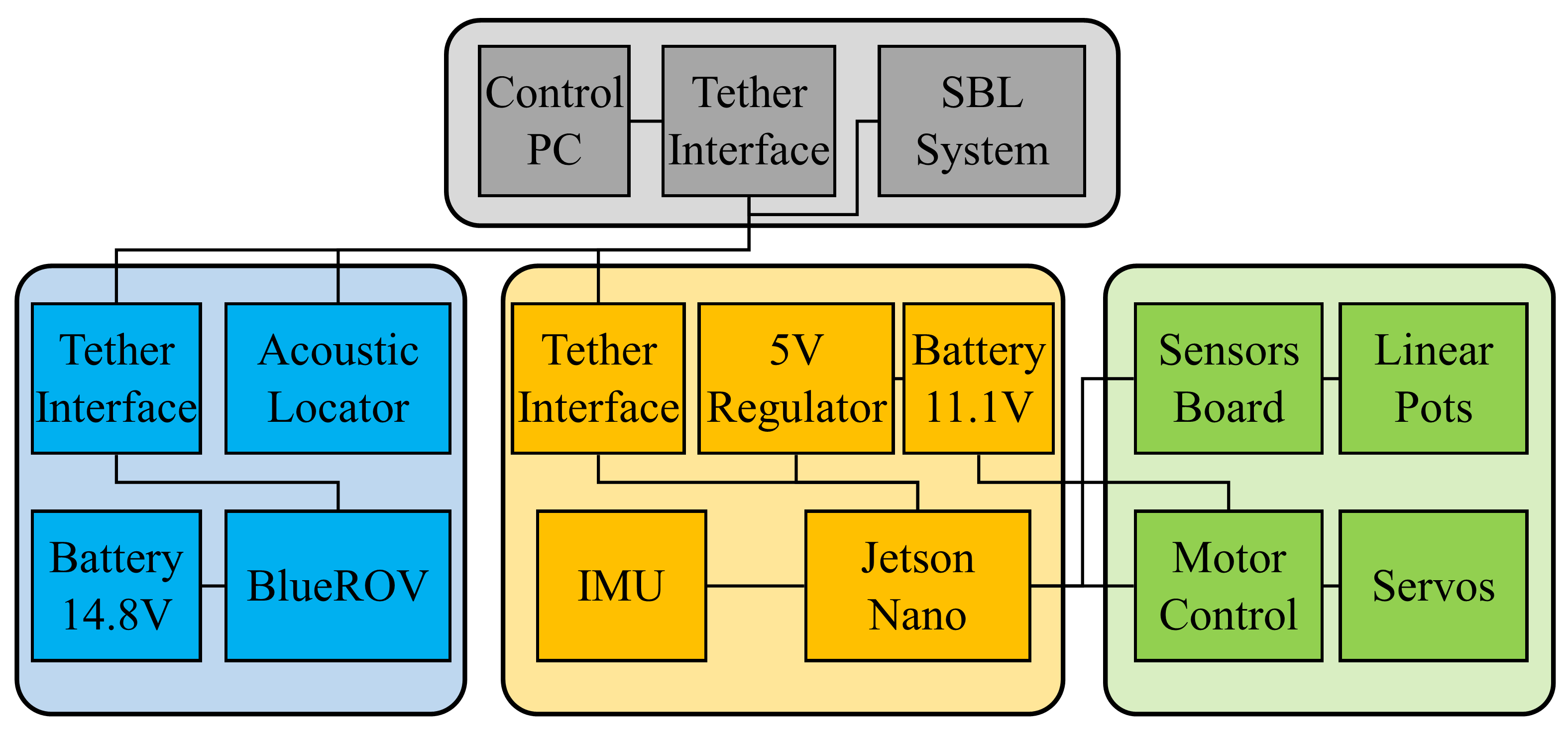
Figure 6: Electronic Systems Schematic

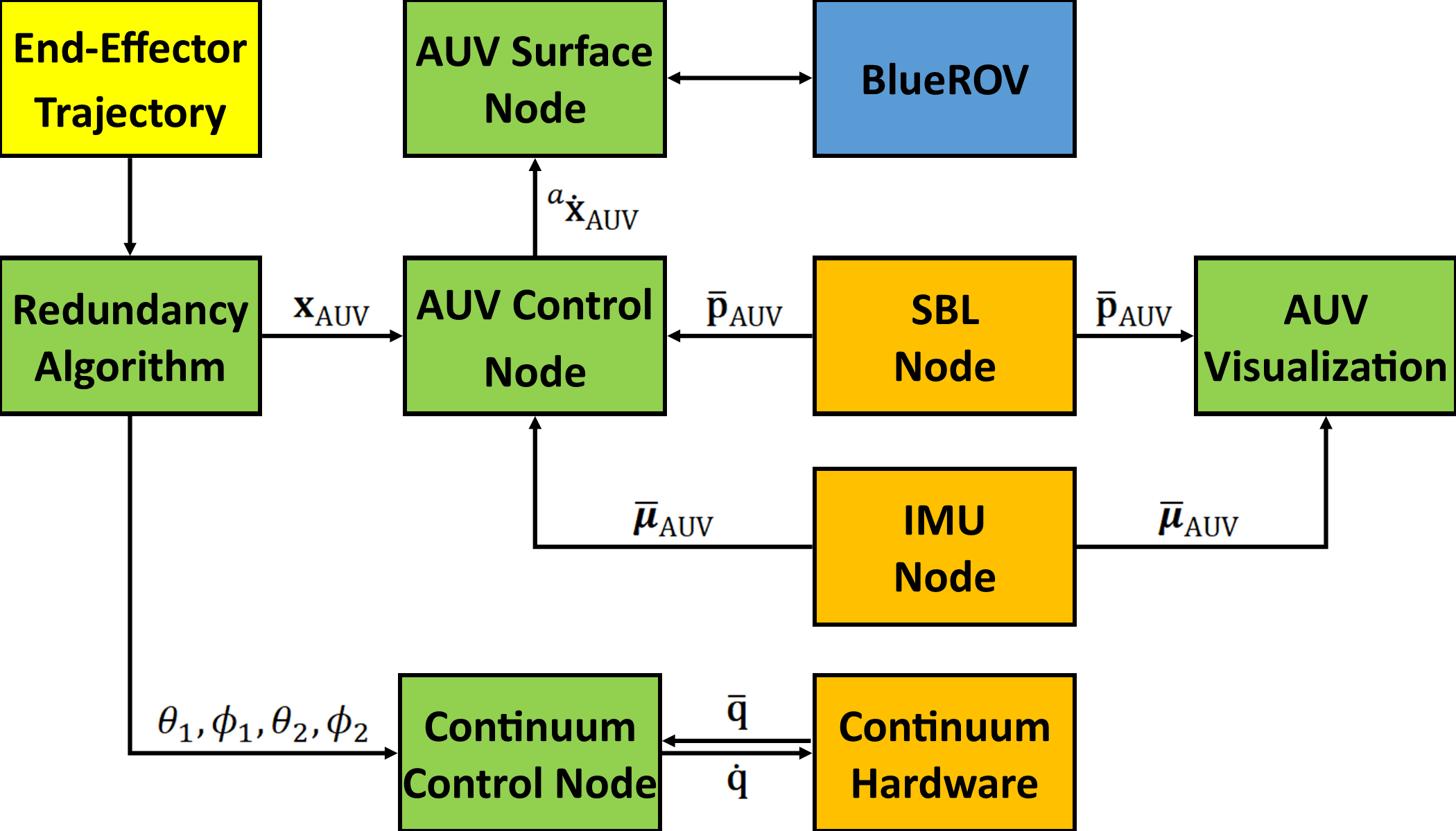
Figure 7: Software Schematic

V Experimental Validation

Initial testing of the arm and AUV system was done using teleoperational control using a separate gamepad controller for each. Alternatively, commands for the continuum arm can be generated using a modified node which receives terminal input and publishes continuum state messages according to a smooth fifth order polynomial. These tests demonstrate the plausibility of using the underwater continuum manipulator for basic manned field tasks, although integration with a gripper or other tool was not carried out for this paper.

In order to demonstrate the potential of the redundancy resolution algorithm, a real world autonomous experiment was carried out in the Davidson Laboratory towing tank at Stevens Institute of Technology. This location was chosen because of its controlled environment, close proximity, and ease of deployment. In this experiment, the acoustic SBL positioning system and VectorNav IMU provide the AUV position and orientation estimates which are used as low-level control feedback, and the desired AUV pose is generated in real time via Algorithm 1. For simplicity, the roll and pitch of the AUV are neglected from the redundancy resolution algorithm as well as the AUV controller, which is a reasonable assumption since the AUV autopilot is designed to stabilize the AUV in an upright position.

The robot’s task for this experiment is to trace out the circular trajectory with its end effector in real time, as described in Sections II-C and III. This task tests the path generation capabilities of the redundancy resolution algorithm and the functionality of the continuum manipulator. An additional objective function is added to minimize the distance between the AUV origin and the point $\mathbf{p}_{\text{anchor}}$ according to (30). This helps keep the AUV close to the center of the circle and incentivizes use of the manipulator as much as possible. The GCS is located at the surface of the water and at the centroid of the SBL locator sensors with the Z axis aligned directly upwards.

A time lapse of the end effector trajectory can be seen in Figure 8. In this figure, the real trajectory of the arm is found by manually selecting the tip of the arm every 100 frames of the video playback. The color of the line also indicates the time progression of the trajectory, with red and yellow values corresponding to earlier in the trajectory and blue and purple values corresponding to later in the trajectory. The best-fit circle (in red) is found using the least squares method over the trajectory coordinates, which approximates the desired task trajectory. A yellow cross represents the current position of the end effector in each frame for reference.

In addition, Figure 2 provides a series of side-by-side comparisons of the AUV and end effector position estimate along with the real-world position. The estimate is visualized using RViz with ROS data from the sensor measurements and manipulator state. The coordinate frames representing the GCS, AUV origin, end effector frame, and the fixed point $\mathbf{p}_{\text{anchor}}$ can be seen in the visualization. This shows that there are slight differences between the robot’s estimated pose and its actual pose, but these differences are not significant enough to prevent control of the AUV.

These results show the redundancy resolution algorithm is capable of real time path generation and tracking. The error in tracing the circle is notable, but can be attributed to the simplicity of the AUV controller. The experimental results shows the AUV exhibits overshoot particularly when strafing along the local Y axis, which could be mitigated by a more advanced low-level vehicle controller that deals with the SBL positioning feedback with high noise. Some of this overshoot can be attributed to noise in the position feedback; a simple Kalman filter for the position estimate was tested, but this caused a significant delay in the estimate. In addition, inertial and hydrodynamic effects are neglected in the controller; the impact of these can be seen by the pitching and rolling of the AUV as it follows the trajectory. Ultimately, a more robust and comprehensive low-level AUV controller could alleviate much of the error, but the development of this low-level vehicle controller was not the focus of this paper.

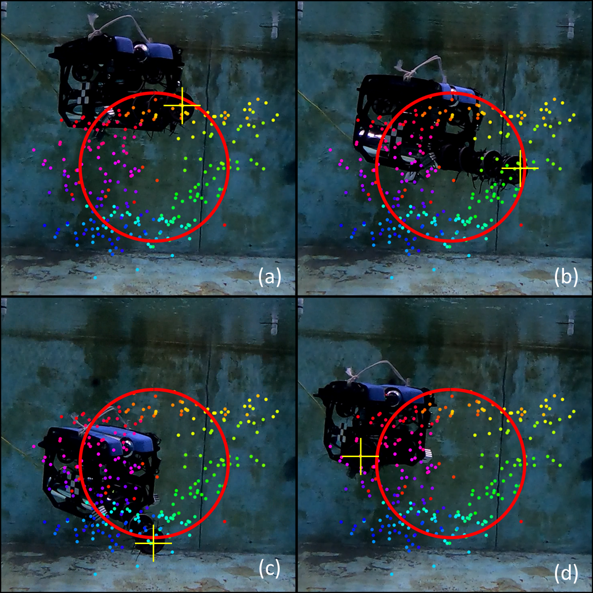
Figure 8: AUV control trajectory, with end effector position and best-fit circle overlay. Progression of trajectory follows the path (a), (b), (c), then (d).

VI Conclusion

This paper introduces an algorithm for solving the redundancy of a free-floating AUV and manipulator system, and provides experimental results that demonstrate the algorithm in real time. The kinematics and total Jacobian matrix are mathematically derived as part of the redundancy resolution method, and the algorithm to generate an optimal trajectory is provided. Choice of the objective function for subtask optimization is discussed, which can be modified based on desired parameters. Mechanical, electrical, and software designs are introduced to explain functionality and allow the system to be reproduced experimentally. The experimental results are then presented, with potential sources of error in the AUV control discussed as well.

Future work could include improvements to the AUV low-level controller to reduce error in tracking and make the system more useful for practical tasks. Further refinement of algorithm parameters may also allow the robot to better balance speed and performance, as well as improve optimization of secondary objectives. Additional objectives can be added to factor in how close the end effector is to its goal or change priorities during execution. One example objective function to investigate in the future could be the one that priorities based on the different levels of accuracy and uncertainties among different kinematic joints. Multi-manipulator planning may also be a lucrative research topic, with potential applications including dexterous underwater manipulation, perching, or climbing.

References

- [1] J. A. Trotter, C. Pattiaratchi, P. Montagna, M. Taviani, J. Falter, R. Thresher, A. Hosie, D. Haig, F. Foglini, Q. Hua et al., “First rov exploration of the perth canyon: Canyon setting, faunal observations, and anthropogenic impacts,” Frontiers in Marine Science, vol. 6, no. 173, 2019.
- [2] V. H. Fernandes, A. A. Neto, and D. D. Rodrigues, “Pipeline inspection with auv,” in IEEE/OES Acoustics in Underwater Geosciences Symposium (RIO Acoustics), 2015, pp. 1–5.
- [3] P. Rundtop and K. Frank, “Experimental evaluation of hydroacoustic instruments for rov navigation along aquaculture net pens,” Aquacultural Engineering, vol. 74, pp. 143–156, 2016. [Online]. Available: https://www.sciencedirect.com/science/article/pii/S0144860916300012
- [4] L. Paull, S. Saeedi, M. Seto, and H. Li, “Auv navigation and localization: A review,” IEEE Journal of oceanic engineering, vol. 39, no. 1, pp. 131–149, 2013.
- [5] J. Jung, Y. Lee, D. Kim, D. Lee, H. Myung, and H.-T. Choi, “Auv slam using forward/downward looking cameras and artificial landmarks,” in 2017 IEEE Underwater Technology (UT). IEEE, 2017, pp. 1–3.
- [6] J. Aulinas, M. Carreras, X. Llado, J. Salvi, R. Garcia, R. Prados, and Y. R. Petillot, “Feature extraction for underwater visual slam,” in OCEANS 2011 IEEE-Spain. IEEE, 2011, pp. 1–7.
- [7] C. Lodovisi, P. Loreti, L. Bracciale, and S. Betti, “Performance analysis of hybrid optical–acoustic auv swarms for marine monitoring,” Future Internet, vol. 10, no. 7, p. 65, 2018.
- [8] J. McConnell, J. D. Martin, and B. Englot, “Fusing concurrent orthogonal wide-aperture sonar images for dense underwater 3d reconstruction,” in 2020 IEEE/RSJ International Conference on Intelligent Robots and Systems (IROS). IEEE, 2020, pp. 1653–1660.
- [9] J. McConnell and B. Englot, “Predictive 3d sonar mapping of underwater environments via object-specific bayesian inference,” in 2021 IEEE International Conference on Robotics and Automation (ICRA). IEEE, 2021, pp. 6761–6767.
- [10] J. McConnell, F. Chen, and B. Englot, “Overhead image factors for underwater sonar-based slam,” IEEE Robotics and Automation Letters, vol. 7, no. 2, pp. 4901–4908, 2022.
- [11] J. Wang, F. Chen, Y. Huang, J. McConnell, T. Shan, and B. Englot, “Virtual maps for autonomous exploration of cluttered underwater environments,” arXiv preprint arXiv:2202.08359, 2022.
- [12] G. Marani, S. K. Choi, and J. Yuh, “Underwater autonomous manipulation for intervention missions auvs,” Ocean Engineering, vol. 36, no. 1, pp. 15–23, 2009, autonomous Underwater Vehicles. [Online]. Available: https://www.sciencedirect.com/science/article/pii/S002980180800173X
- [13] P. J. Sanz, P. Ridao, G. Oliver, C. Melchiorri, G. Casalino, C. Silvestre, Y. Petillot, and A. Turetta, “Trident: A framework for autonomous underwater intervention missions with dexterous manipulation capabilities,” IFAC Proceedings Volumes, vol. 43, no. 16, pp. 187–192, 2010.
- [14] J. J. Fernández, M. Prats, P. J. Sanz, J. C. García, R. Marin, M. Robinson, D. Ribas, and P. Ridao, “Grasping for the seabed: Developing a new underwater robot arm for shallow-water intervention,” IEEE Robotics & Automation Magazine, vol. 20, no. 4, pp. 121–130, 2013.
- [15] O. Khatib, X. Yeh, G. Brantner, B. Soe, B. Kim, S. Ganguly, H. Stuart, S. Wang, M. Cutkosky, A. Edsinger, P. Mullins, M. Barham, C. R. Voolstra, K. N. Salama, M. L’Hour, and V. Creuze, “Ocean one: A robotic avatar for oceanic discovery,” IEEE Robotics Automation Magazine, vol. 23, no. 4, pp. 20–29, 2016.
- [16] R. Conti, F. Fanelli, E. Meli, A. Ridolfi, and R. Costanzi, “A free floating manipulation strategy for autonomous underwater vehicles,” Robotics and Autonomous Systems, vol. 87, pp. 133–146, 2017.
- [17] J. E. Manley, S. Halpin, N. Radford, and M. Ondler, “Aquanaut: A new tool for subsea inspection and intervention,” in OCEANS 2018 MTS/IEEE Charleston, 2018, pp. 1–4.
- [18] D. Youakim, P. Ridao, N. Palomeras, F. Spadafora, D. Ribas, and M. Muzzupappa, “Moveit!: autonomous underwater free-floating manipulation,” IEEE Robotics & Automation Magazine, vol. 24, no. 3, pp. 41–51, 2017.
- [19] D. Youakim, P. Cieslak, A. Dornbush, A. Palomer, P. Ridao, and M. Likhachev, “Multirepresentation, multiheuristic a* search-based motion planning for a free-floating underwater vehicle-manipulator system in unknown environment,” Journal of Field Robotics, vol. 37, no. 6, pp. 925–950, 2020.
- [20] P. Ridao, M. Carreras, D. Ribas, P. J. Sanz, and G. Oliver, “Intervention auvs: the next challenge,” Annual Reviews in Control, vol. 40, pp. 227–241, 2015.
- [21] J. Liu, S. Iacoponi, C. Laschi, L. Wen, and M. Calisti, “Underwater Mobile Manipulation: A Soft Arm on a Benthic Legged Robot,” IEEE Robotics & Automation Magazine, vol. 27, no. 4, pp. 12–26, Dec 2020.
- [22] M. Cianchetti, M. Calisti, L. Margheri, M. Kuba, and C. Laschi, “Bioinspired locomotion and grasping in water: The soft eight-arm octopus robot,” Bioinspiration & Biomimetics, vol. 10, 03 2015.
- [23] Z. Gong, B. Chen, J. Liu, X. Fang, Z. Liu, T. Wang, and L. Wen, “An opposite-bending-and-extension soft robotic manipulator for delicate grasping in shallow water,” Frontiers in Robotics and AI, vol. 6, 04 2019.
- [24] J. L. Sitler and L. Wang, “A Modular Open-Source Continuum Manipulator for Underwater Remotely Operated Vehicles,” Journal of Mechanisms and Robotics, vol. 14, no. 6, 04 2022. [Online]. Available: https://doi.org/10.1115/1.4054309
- [25] F. Flacco, A. De Luca, and O. Khatib, “Motion control of redundant robots under joint constraints: Saturation in the null space,” in IEEE International Conference on Robotics and Automation, 2012, pp. 285–292.
- [26] H. Xing, Z. Gong, L. Ding, A. Torabi, J. Chen, H. Gao, and M. Tavakoli, “An adaptive multi-objective motion distribution framework for wheeled mobile manipulators via null-space exploration,” Mechatronics, vol. 90, no. 102949, 2023. [Online]. Available: https://www.sciencedirect.com/science/article/pii/S0957415823000053
- [27] L. Wang, “Open source modular continuum robot project,” https://longwang.in/modular-continuum-manipulator/, 2022, accessed: 2023-01-30.
- [28] T. F. Chan and R. V. Dubey, “A weighted least-norm solution based scheme for avoiding joint limits for redundant joint manipulators,” IEEE Transactions on Robotics and Automation, vol. 11, no. 2, pp. 286–292, 1995.
- [29] A. Liegeois et al., “Automatic supervisory control of the configuration and behavior of multibody mechanisms,” IEEE transactions on systems, man, and cybernetics, vol. 7, no. 12, pp. 868–871, 1977.
- [30] Y. Liu, J. Zhao, and B. Xie, “Obstacle avoidance for redundant manipulators based on a novel gradient projection method with a functional scalar,” in 2010 IEEE International Conference on Robotics and Biomimetics. IEEE, 2010, pp. 1704–1709.
- [31] I. D. Walker and S. I. Marcus, “Subtask performance by redundancy resolution for redundant robot manipulators,” IEEE Journal on Robotics and Automation, vol. 4, no. 3, pp. 350–354, 1988.
- [32] Blue Robotics, Inc., https://bluerobotics.com/, accessed: 2023-01-30.
- [33] S. Soylu, A. Proctor, R. Podhorodeski, C. Bradley, and B. Buckham, “Precise trajectory control for an inspection class rov,” Ocean Engineering, vol. 111, pp. 508–523, 2016. [Online]. Available: https://www.sciencedirect.com/science/article/pii/S002980181500459X
- [34] Open Robotics, “ROS - Robot Operating System,” https://www.ros.org, accessed: 2023-01-30.
- [35] J. McConnell, “BlueROV2 Heavy ROS Package,” https://github.com/jake3991/Argonaut, accessed: 2023-01-30.