Faculty Induction Programme (FIP-3)
 
 
1st June 2022 – 2nd July 2022
 
 
 
Topic: Effect of Spreading Knowledge Centers – A Physics-based Approach
 
 
 
Submitted as partial fulfilment of UGC sponsored
Faculty Induction Programme
 
 
 
By
Saurish Chakrabarty
Department of Physics
Acharya Prafulla Chandra College
West Bengal State University
 
CENTRE FOR PROFESSIONAL DEVELOPMENT IN HIGHER EDUCATION
UNIVERSITY OF DELHI
DELHI-110007

Declaration of Originality

Name: Saurish Chakrabarty
Subject: Physics
College: Acharya Prafulla Chandra College
University: West Bengal State University
 

Title of the paper: Effect of Spreading Knowledge Centers – A Physics-based Approach
 

I hereby declare that the project report/paper titled “Effect of Spreading Knowledge Centers – A Physics-based Approach” that I am submitting to fulfill the requirement towards completion of my Faculty Induction Programme (FIP-3) (1st June 2022 2nd July 2022), at CPDHE, University of Delhi, represents my original work and that I have used no other sources except those that I have indicated in the references. All data, tables, figures and text citations which have been reproduced from any other source, including the internet, have been explicitly acknowledged as such. I am aware of the consequences of non-compliance of my above declaration.
 

Saurish Chakrabarty
 
Kolkata, West Bengal
 
Date: June 20, 2022

Abstract

We use a simple physics-inspired model to get an idea about how to enhance the speed with which a society becomes educated if we strategically place our knowledge spreading centers (teachers or educational institutions). We study knowledge spreading using the Ising model, a well-studied model used in physics, specifically statistical mechanics, to describe the phenomenon of ferromagnetism. In the social context, up and down spins are mapped to knowledgeable and ignorant individuals. We introduce some knowledgeable individuals into an otherwise ignorant society and see how their number increases with time, when evolved using the Metropolis algorithm. We find that the knowledge of the society grows faster when the initial group of knowledgeable individuals is maximally spread out. We quantify this effect using the doubling time and look at the distribution of the doubling time as a function of “temperature”. In the social context, the energy is identified as the (lack of) happiness of neighbours and temperature is a parameter that quantifies how important happiness is in the society. We point out several limitations of this study in order to facilitate future research.

Keywords
Ising model, knowledge spreading, doubling time, sociophysics, econophysics

1 Background and Introduction

The Ising model [3] was introduced as a simple model by Lenz in 1920 to explain ferromagnetism, a phenomenon in which below a certain critical temperature, local microscopic magnetic moments spontaneously align to give rise to a macroscopic magnetization. In this work, we use this model in a social setting where the Ising model can be seen as a model that describes a society which veers towards an equilibrium state where knowledge that is initially available to a small set of individuals in a population, later gets distributed among a large fraction of the population. We begin with a brief review of the Ising model in the standard statistical mechanistic setting. This model is described on a $d$-dimensional regular lattice with “spins”, $\left\{S_{i}\right\}$, residing on every lattice site. This work focuses on $d=2$ (two spatial dimensions). Each spin can take one of two values, $\pm 1$, (“up” and “down”).

Applications of the Ising model and its variants to social settings are not new. For a short but excellent review see Ref. [12] and the references therein. For another, more exhaustive review of physics-inspired models in financial economics, including the Ising model, see Ref. [10]. The Ising model has been used in the past to understand damage spreading.[13] It has also been used to understand patterns in tax evasion.[14] In this context, the up and down spins were used to represent “honest” tax payers and “cheaters”. Self organization in the financial markets can also be studied using the Ising model.[15] In this work, stochastic evolution was used instead of the standard Hamiltonian formulation. Talking about self organization, it is important to point out that self organization, especially the phenomenon self organized criticality, is a very important and interesting branch of the statistical mechanics of complex systems and explains a lot of universality that we see in nature.[1] A model based on the Ising model has been used to understand the role of social impact.[5] Here, the Ising variables represented the “opinions” and there were two kinds of coupling constants “persuasiveness” and “support”.

The Ising model is described by the following simple Hamiltonian.

$${\cal H}=-J\sum_{\langle i,j\rangle}S_{i}S_{j}-h\sum_{i}S_{i}$$ (1)

[For a reader unaware of what the Hamiltonian is, it represents the energy function. When thermal effects are not important, a system minimizes its energy, and when they are important, there is a balance between minimization of the energy and maximization of the entropy (tendency to approach a distribution in which the number of microscopic configurations is high, $i.e.$, the system is confused).] The coupling constant $J$ is taken to be positive in the ferromagnetic Ising model and sets the scale of energies. The first term is a sum over nearest neighbours (denoted by the angular brackets) and to satisfy this term, nearest neighbours must have the same spin. Here, the word satisfy refers to allowing it to contribute the lowest possible energy. When $h=0$, the model results in a ground state where all the spins point in the same direction. When $h\neq 0$, in the ground state, all the spins take the sign of $h$. The constant, $h$, therefore, plays the role of a magnetic field and spins align in the direction of the magnetic field. Generalizations of the two constants give rise to many interesting phenomena such as antiferromagnetism, spin glasses and localization-delocalization transitions.

Equilibrium properties of the Ising model at some external temperature, $T$, (canonical ensemble) are obtained by calculating the partition function,

$$Z=\mbox{Tr}~{}e^{-\beta{\cal H}},$$ (2)

where $\beta=\frac{1}{k_{B}T}$, $k_{B}$ being the Boltzmann constant and the symbol Tr (trace) represents the sum over all possible configurations.

The partition function for the Ising model was calculated by Ising in one spatial dimension [3] and by Onsager in two spatial dimensions [7]. Onsager used the well-known transfer matrix method that was invented a few years ago and played a role in popularizing the method which later proved to be a useful tool in solving many problems in all areas of physics, including statistical mechanics, particularly in the area of complex systems. It is generally believed that a closed-form analytical solution of the three-dimensional Ising model is not possible. In two and more dimensions, the Ising model shows a transition from a low-temperature ferromagnetic phase (most spins pointing in the same direction) to a high-temperature paramagnetic phase (no preferred direction of the spins). This transition occurs at a critical temperature, $T_{c}$, that depends on the number of spatial dimensions.

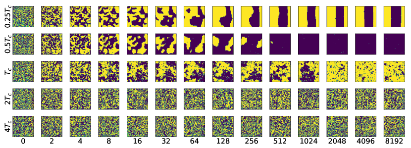
Figure 1: Configurations of the two-dimensional Ising model with periodic boundary conditions, evolved using the Metropolis algorithm, starting from a random configuration, with $J=1$ and $h=0$. Each row corresponds to a fixed temperature that is written on the left of the row. The number of Monte Carlo cycles increases from left to right and is written at the bottom of each column. For the two-dimensional Ising model, $T_{c}\approx 2.269J/k_{B}$ and the equilibrium configurations below this temperature are ferromagnetic and above this temperature are paramagnetic. As is clear from the data, in the ferromagnetic phase, presence of domain walls across the system costs very little energy and can last very long.

Configurations corresponding to the equilibrium distribution at a given temperature can be sampled using the Metropolis algorithm.[6] In this method, a spin is chosen at random and flipped. If this causes a reduction in the energy, then the move is accepted. If, on the other hand there is a rise in the energy, then the move is accepted with probability, $e^{-\beta\Delta E}$, where $\Delta E$ is the increase in energy. This process results in a distribution of configurations such that the probability of having a configuration with energy $\cal H$ is $\frac{1}{Z}e^{-\beta{\cal H}}$. Configurations obtained by evolution using this algorithm are shown in Figs. 1 and 2. In Fig. 1, we have chosen a random initial configuration, $i.e$, each spin can be either up or down, with equal probability. In Fig. 2, we start with initial configurations in which all spins are down.

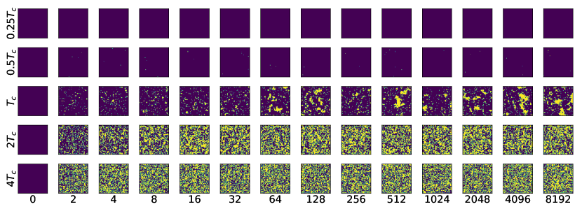
Figure 2: Configurations starting from a configuration with all down spins. All other details are the same as Fig. 1. Ignoring the vertical domain wall at the lowest temperature in Fig. 1 and with the up-down symmetry in the Hamiltonian when $h=0$, the configurations on the last column are statistically similar to the corresponding figures on the last column of Fig. 1.

2 Application to Knowledge Spreading

The Ising model can be used to describe any two-level system. In the application we have in mind, it will be convenient to work with variables which take values in $\{0,1\}$ instead of $\{-1,+1\}$. This change is achieved by the following change of variables.

$$\sigma_{i}=\frac{S_{i}+1}{2}\mbox{, or equivalently, }S_{i}=2\sigma_{i}-1$$ (3)

We apply the Ising model to the following social scenario. Consider a society with $N=L\times L$ individuals, each occupying a site on a square grid of side $L$. (These $N$ sites could be occupied by $N$ households as well.) Each person is either aware or unaware of some fact, $i.e$., can be in two states – one or zero (up or down). The person is “happy” if surrounded by people in the same state. We can characterize each connection (bond) with its happiness. Lower the energy, higher is the happiness. The individuals (or bonds) keep evolving (fighting or struggling) in the quest for happiness.

It is clear that the above setup has the ingredients to be modeled using the Ising model with zero field. Each person has a knowledge level $\sigma\in\{0,1\}$ and the Hamiltonian $\cal H$ in Eq. 1, can be thought to represent the negative of happiness ($i.e.$, sadness). The environment introduces fluctuations and enforces some of their statistical properties. These are controlled by the “temperature”, $T$. At a low temperature, the society veers towards a state with lowest energy (maximum happiness). At extremely high temperatures, the system tends to become maximally disordered (maximum entropy). In this situation, states of neighbours are uncorrelated (people do not care about each other and are not affected by their state). Happiness in the society is not important.

Another interesting point to note is that the situation in which every person in the society is knowledgeable has the same total happiness as the situation in which no person is. More generally, there is a symmetry that flipping the states of all the individuals does not affect the society’s overall energy or happiness.

The above description is incomplete without the specification of the boundary conditions. The society has periodic boundary conditions. The exit at the north boundary is the entry through the south boundary and vice versa. The same is true for the east and west boundaries. This kind of boundary condition has numerical advantages and finite size effects are small. In addition, all sites are equivalent. Everyone has the same number of neighbours. No location can be called a central location and no location can be called a boundary. In what follows, we will destroy this beautiful spatial homogeneity.

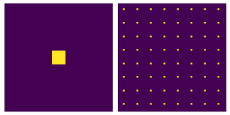
Figure 3: The two chosen starting configurations – centered (left) and distributed (right), shown here with $n_{s}=64$.

We now consider the scenario in which $n_{s}=l_{s}\times l_{s}$ knowledgeable people are introduced into the society in which everyone is ignorant. These $n_{s}$ individuals stay knowledgeable forever. We look at the effect of their locations on the future knowledge content of the society. We evolve the society using the Metropolis algorithm and calculate the time (Monte Carlo steps) taken to double the number of knowledgeable individuals. We denote this by time by $\tau$. One Monte Carlo step corresponds to $N$ spin-flip (knowledge-flip) attempts. We compare the following two situations.

1. In the beginning all the knowledgeable individuals stay close by. They occupy all sites in a $l_{s}\times l_{s}$ square somewhere in the system, as shown in the left panel of Fig. 3.

2. In the beginning all the knowledgeable individuals stay in a regular array, as far from each other as possible, as shown in the right panel of Fig. 3.

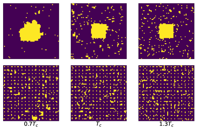
Figure 4: Configurations after the doubling time, $\tau$. The two top and the bottom rows correspond to centered and distributed starting configurations, respectively. The configurations shown are for $n_{s}=256$. Each column correspond to a fixed temperature that is mentioned at the bottom.

3 Details of the Study and Results

We focus on a system with $N=4096$ sites. The initial number of knowledgeable individuals, $n_{s}$, was taken from the set $\{16,64,256\}$. The temperature, $T$, was chosen from the set $\{0.7T_{c},T_{c},1.3T_{c}\}$. The choice of these parameters were determined only by the time and the computational resources that were available for doing the work. More of these parameter values should be explored in future.

In Fig. 4, we see the temperature dependence of the pattern in which knowledge spreads in the above two situations. Larger clusters of knowledge centers are seen at lower temperatures. The starting configuration had $n_{s}=256$ for the snapshots shown in this figure.

In Fig. 5, we see that when $n_{s}=16$, the locations and spread of the distributions are affected slightly by the choice of the starting configuration, the blue-solid and red-dashed lines representing the initially centered and spread-out knowledge centers respectively. The distribution with the spread-out initial configuration is narrower and peaked at a lower time. The effect becomes less significant with increasing temperature. If we look at higher values of $n_{s}$, the effects become more pronounced. These details are further supported by the numbers shown in Table 1. The means and standard deviations of the data sets are mentioned here. More importantly, the sizes of the data sets are also given.

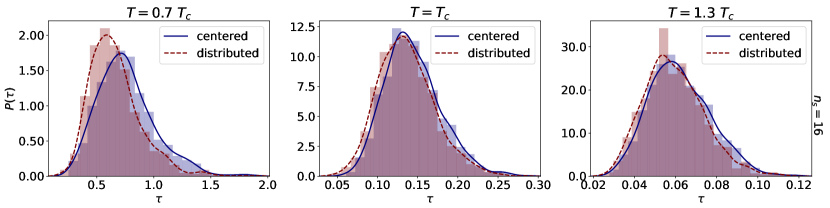
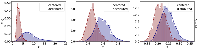
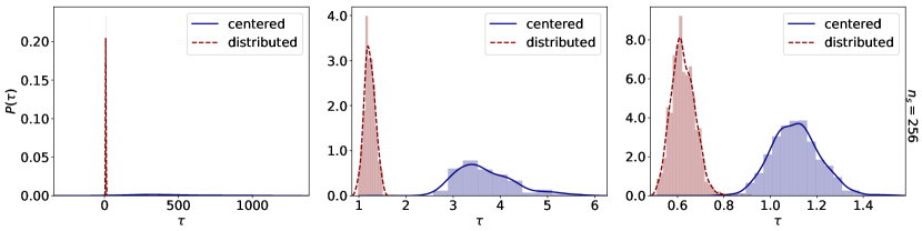
Figure 5: The distributions of the doubling time, $\tau$. In the top row, there are $n_{s}=16$ knowledgeable people initially. In the middle row, $n_{s}=64$. Finally, in the bottom row, $n_{s}=256$. The three columns are for three different temperatures (mentioned at the top of each column). In each of the three panels, centered and distributed starting seeds have been shown in different colors. The lines are obtained via Kernel Density Estimation (computed using the $pandas$ module in $python$ [9]). The choice of this method was done arbitrarily with a purpose to have a guiding trend line for the reader (any other spline algorithm would have also served our purpose and due to the limited size of the data set used, features other than the mean and variance of the data should not be taken too seriously).

$\bm{n_{s}}$	$\bm{T}$	Initial location of knowledge centers	$\bm{\langle\tau\rangle}$	$\bm{\sigma_{\tau}}$	Size of data set
16	0.7$T_{c}$	centered	0.758	0.252	1000
		distributed	0.662	0.222	1000
	$T_{c}$	centered	0.144	0.0348	1000
		distributed	0.136	0.0347	1000
	1.3$T_{c}$	centered	0.0622	0.0149	1000
		distributed	0.0593	0.0144	1000
64	0.7$T_{c}$	centered	8.66	4.35	1000
		distributed	3.07	1.02	1000
	$T_{c}$	centered	0.597	0.0919	1000
		distributed	0.462	0.0687	1000
	1.3$T_{c}$	centered	0.245	0.0316	1000
		distributed	0.212	0.0284	1000
256	0.7$T_{c}$	centered	442	260	38
		distributed	8.67	1.97	100
	$T_{c}$	centered	3.67	0.604	142
		distributed	1.23	0.112	100
	1.3$T_{c}$	centered	1.11	0.105	1000
		distributed	0.624	0.0489	1000

Table 1: Information about the data set generated from simulation: Means and standard deviations of the doubling times are shown in addition to the sizes of the data set used (which are small for some sets of parameters).

4 Conclusion

To conclude, we see that a simple physics-inspired model can be used to give us an idea about how to enhance the speed with which a society becomes educated. A good strategy adopted to place our knowledge spreading centers (teachers) plays an important role. In an alternate interpretation in which the sites in our model are occupied by households, the initial centers of knowledge may represent educational institutions, libraries, news agencies or any other institution depending on the kind of knowledge we wish to focus on. Our results suggest that a good strategy is to spread out the knowledge centers as much as possible. Environmental factors (here “temperature”) play a big role. When the temperature is low, the choice of strategy has a much profound effect, $i.e.$, it is significantly better to spread out the teachers. The difference gets washed out with “thermal” fluctuations. Lastly, if we have more resources, it is even more fruitful, and therefore important, to adopt the better strategy of spreading out our resources.

5 Limitations and Possible Extensions

This work was done as a part of a Faculty Induction Programme and very little time could be spent on it. As such, the following areas should be explored more exhaustively in order to establish the universal applicability of the results.

1. System size dependence – Even though the system size used here was not too small, for completeness an analysis of the effect of the system size should be done in order to have an idea of the smallest system sizes beyond which the variables of interest have similar statistical properties.

2. The effect of other kinds of boundary conditions can be explored – there are many possibilities here.

3. Dynamics dependence – Other than the Metropolis algorithm, many alternative dynamics protocols could be used to evolve the Ising configurations, such as Glauber dynamics[2] and Kawasaki dynamics[4]. If the results are qualitatively and/or quantitatively different, then a study on which of the dynamics is most appropriate should be done.

4. If possible, a comparison may be made to trends seen in some available data on knowledge spreading and look for the universal features in such data sets.

5. The need for promotion of the number of possible levels of knowledge could be explored. Two possible generalizations can be made.

   1. Multiple areas or discrete levels of knowledge – Potts model.[8]

   2. Multiple components of knowledge each having a continuous (real number) level – $n$ component Heisenberg model, also known as the $O(n)$ model.[11]

6. Finally, in a real situation, people are not arranged in a regular grid. The effect of removing the grid may also be looked at. This may be taken care of by studying a system with varying bond lengths or equivalently by adding disorder to the coupling constants.

Acknowledgment

The author would like to thank the Centre for Professional Development in Higher Education, Delhi University and the other organizers of the Faculty Induction Programme that forced the author to come up with an interdisciplinary research topic and obtain some preliminary results. This may open a future research avenue for the author to explore.

- [1] Per Bak, Chao Tang, and Kurt Wiesenfeld. Self-organized criticality. Physical Review A, 38:364–374, 1988.
- [2] Roy J. Glauber. Time‐Dependent Statistics of the Ising Model. Journal of Mathematical Physics, 4(2):294–307, 1963.
- [3] Ernst Ising. Beitrag zur Theorie des Ferromagnetismus. Zeitschrift für Physik, 31:253, 1925.
- [4] Kyozi Kawasaki. Diffusion Constants near the Critical Point for Time-Dependent Ising Models. I. Physical Review, 145:224–230, 1966.
- [5] G. A. Kohring. Ising Models of Social Impact: the Role of Cumulative Advantage. Journal de Physique I France, 6(2):301–308, 1996.
- [6] Nicholas Metropolis, Arianna W. Rosenbluth, Marshall N. Rosenbluth, Augusta H. Teller, and Edward Teller. Equation of State Calculations by Fast Computing Machines. The Journal of Chemical Physics, 21(6):1087–1092, 1953.
- [7] Lars Onsager. Crystal Statistics. I. A Two-Dimensional Model with an Order-Disorder Transition. Physical Review, 65:117–149, 1944.
- [8] R. B. Potts. Some generalized order-disorder transformations. Mathematical Proceedings of the Cambridge Philosophical Society, 48(1):106109, 1952.
- [9] pandas.DataFrame.plot.kde pandas 1.4.2 documentation. https://pandas.pydata.org/docs/reference/api/pandas.DataFrame.plot.kde.html, Last accessed on June 19, 2022.
- [10] Didier Sornette. Physics and financial economics (1776-2014): puzzles, Ising and agent-based models. Reports on Progress in Physics, 77(6):062001, 2014.
- [11] H. E. Stanley. Dependence of critical properties on dimensionality of spins. Physical Review Letters, 20:589–592, 1968.
- [12] D. Stauffer. Social applications of two-dimensional Ising models. American Journal of Physics, 76(4):470–473, 2008.
- [13] Pontus Svenson and Desmond A. Johnston. Damage spreading in small world Ising models. Physical Review E, 65:036105, 2002.
- [14] Georg Zaklan, Frank Westerhoff, and Dietrich Stauffer. Analysing tax evasion dynamics via the Ising model. Journal of Economic Interaction and Coordination, 4(1):1, 2009.
- [15] W.-X. Zhou and D. Sornette. Self-organizing Ising model of financial markets. The European Physical Journal B, 55(2):175–181, 2007.