Decentralized Model Dissemination Empowered Federated Learning in mmWave Aerial-Terrestrial Integrated Networks

Abstract

It is anticipated that aerial-terrestrial integrated networks incorporating unmanned aerial vehicles (UAVs) mounted relays will offer improved coverage and connectivity in the beyond 5G era. Meanwhile, federated learning (FL) is a promising distributed machine learning technique for building inference models over wireless networks due to its ability to maintain user privacy and reduce communication overhead. However, off-the-shelf FL models aggregate global parameters at a central parameter server (CPS), increasing energy consumption and latency, as well as inefficiently utilizing radio resource blocks (RRBs) for distributed user devices (UDs). This paper presents a resource-efficient FL framework, called FedMoD (federated learning with model dissemination), for millimeter-wave (mmWave) aerial-terrestrial integrated networks with the following two unique characteristics. Firstly, FedMoD presents a novel decentralized model dissemination algorithm that makes use of UAVs as local model aggregators through UAV-to-UAV and device-to-device (D2D) communications. As a result, FedMoD (i) increases the number of participant UDs in developing FL model and (ii) achieves global model aggregation without involving CPS. Secondly, FedMoD reduces the energy consumption of FL using radio resource management (RRM) under the constraints of over-the-air learning latency. In order to achieve this, by leveraging graph theory, FedMoD optimizes the scheduling of line-of-sight (LOS) UDs to suitable UAVs/RRBs over mmWave links and non-LOS UDs to available LOS UDs via overlay D2D communications. Extensive simulations reveal that decentralized FedMoD offers same convergence rate performance as compared to conventional FL frameworks.

I Introduction

Unmanned aerial vehicles (UAVs) are expected to have a significant impact on the economy by 2026 with a projected global market value of US$59.2 billion, making the inclusion of UAVs critical in beyond 5G cellular networks [1]. There are several unique features of UAV-mounted communication platforms, including the high likelihood of establishing line-of-sight connections with ground nodes, rapid deployment, and adjustable mobility [2]. With such attributes, UAVs can serve as aerial base stations (BSs) or relays in conjunction with terrestrial base stations, resulting in aerial-terrestrial integrated networks (ATINs). By connecting cell-edge user devices (UDs) to terrestrial cellular networks via aerial BSs or relays, ATINs improve coverage and connectivity significantly [3]. The 3GPP standard also incorporates the use of UAVs as a communication infrastructure to complement terrestrial cellular networks [4]. During current 5G deployment efforts, it has been shown that the millimeter-wave band at 28 GHz is significantly larger and more capable than the sub-6 GHz band. At the same time, air-to-ground communications have the advantage of avoiding blockages and maintaining LOS connectivity as a result of UAV’s high altitude and flexibility. [5]. Therefore, the mmWave band is suitable for deploying high-capacity ATINs in the next-generation cellular networks.

A data-driven decision making process enables wireless networks to manage radio resources more efficiently by predicting and analyzing several dynamic factors, such as users’ behavior, mobility patterns, traffic congestion, and quality-of-service expectations. Data-driven radio resource management (RRM) has gained increasing popularity, thanks to the expansion of wireless sensing applications, the availability of enormous data, and the increasing computing capabilities of devices. To train machine learning (ML) models, raw data collected from individual UDs is aggregated in a central parameter server (CPS). As a result, such centralized ML approaches require enormous amounts of network resources to collect raw data from UDs. In addition, centralized ML also impairs users’ privacy since CPS can easily extract sensitive information from raw data gathered from UDs. Recently, Google proposed federated learning (FL) for UDs to collaboratively learn a model without sharing their private data [6]. In FL, UDs update parameters according to their local datasets, and only the most recent parameters are shared with the CPS. Using local models from all participating UDs, the CPS updates global model parameters and shares them with the UDs. The local and global models are adjusted iteratively until convergence. Unlike centralized ML approaches, FL not only protects UD privacy but also improves wireless resource utilization significantly. Nevertheless, the convergence performance of FL in wireless networks significantly depends on the appropriate selection of the participating UDs, based on both channel and data quality, and bandwidth allocation among the selected UDs [7].

The FL framework provides a powerful computation tool for ATINs to make decentralized decisions [8]. UAVs are frequently used as aerial sensors or aerial data collectors in several practical scenarios, and the convergence and accuracy of FL in such use cases can be improved by appropriately exploiting the unique attributes of air-to-ground communication links. For instance, a FL framework was developed for hazardous zone detection and air quality prediction by utilizing UAVs as local learners and deploying a swarm of them to collect local air quality index (AQI) data [9]. A UAV-supported FL framework was also proposed in which a drone visited learning sites sequentially, aggregated model parameters locally, and relayed them to the CPS for global aggregation [9]. Meanwhile, ATINs can also deploy UAVs as aerial BSs with edge computing capabilities. In this context, UAV can provide global model aggregation capability for a large numbers of ground UDs, thanks to its large coverage and high probability of establishing LOS communications [10]. In the aforesaid works, all the local model parameters were aggregated into a single CPS using the conventional star-based FL framework. Although such a star-based FL is convenient, it poses several challenges in the context of ATINs. Firstly, a star-based FL requires a longer convergence time due to the presence of straggling local learners. Recall, the duration of transmission and hovering of a UAV influences its energy consumption, and consequently, increasing the convergence time of FL directly increases the energy consumption of UAVs. This presents a significant challenge for implementing FL in ATINs since UAVs usually have limited battery capacity. In addition, as a result of increased distance and other channel impairments, a number of local learners with excellent datasets may be out of coverage of the central server in practice. The overall learning accuracy of FL models can be severely impacted if these local learners are excluded from the model. The use of star-based FL frameworks in ATINs is also confronted by the uncertainty of air-to-ground communication links resulting from random blocking and the mobility of UAVs. This work seeks to address these challenges by proposing a resource-efficient FL framework for mmWave ATINs that incorporates decentralized model dissemination and energy-efficient UD scheduling.

I-A Summary of the Related Works

In the current literature, communication-efficient FL design problems are explored. In [11], the authors suggested a stochastic alternating direction multiplier method to update the local model parameters while reducing communications between local learners and CPS. In [12], a joint client scheduling and RRB allocation scheme was developed to minimize accuracy loss. To minimize the loss function of FL training, UD selection, RRB scheduling, and transmit power allocation were optimized simultaneously [13]. Numbers of global iterations and duration of each global iteration were minimized by jointly optimizing the UD selection and RRB allocation [14]. Besides, since UDs participating in FL are energy-constrained, an increasing number of studies focused on designing energy-efficient FL frameworks. As demonstrated in [15], the energy consumption of FL can be reduced by uploading only quantized or compressed model parameters from UDs to CPS. Furthermore, RRM enhances energy efficiency of FL in large-scale networks. Several aspects of RRM, such as client scheduling, RRB allocation, and transmit power control, were extensively studied to minimize both communication and computation energy of FL frameworks [16, 17]. An energy-efficient FL framework based on relay-assisted two-hop transmission and non-orthogonal multiple access scheme was recently proposed for both energy and resource constrained Internet of Things (IoT) networks [18]. In the aforesaid studies, conventional star-based FL frameworks were studied. Due to its requirement to aggregate all local model parameters on a single server, the star-based FL is inefficient for energy- and resource-constrained wireless networks.

Hierarchical FL (HFL) frameworks involve network edge devices uploading model parameters to mobile edge computing (MEC) servers for local aggregation, and MEC servers uploading aggregated local model parameters to CPS periodically. The HFL framework increases the number of connected UDs and reduces energy consumption [19]. To facilitate the HFL framework, a client-edge-cloud collaboration framework was explored [20]. HFL was investigated in heterogeneous wireless networks through the introduction of fog access points and multiple-layer model aggregation [21]. Dynamic wireless channels in the UD-to-MEC and MEC-to-CPS hops and data distribution play a crucial role in FL learning accuracy and convergence. Thus, efficient RRM is imperative for implementation of HFL. As a result, existing literature evaluated several RRM tasks, including UD association, RRB allocation, and edge association, to reduce cost, latency, and learning error of HFL schemes [22, 23].

While HFL increases the number of participating UDs, its latency and energy consumption are still hindered by dual-hop communication for uploading and broadcasting local and global model parameters. Server-less FL is a promising alternative to reduce latency and energy consumption. This FL framework allows UDs to communicate locally aggregated models without involving central servers, thereby achieving model consensus. The authors in [24] proposed a FL scheme that relies on device-to-device (D2D) communications to achieve model consensus. However, due to the requirement of global model aggregation with two-time scale FL over both D2D and user-to-CPS wireless transmission, this FL scheme has limited latency improvement. In [25, 26], the authors developed FL model dissemination schemes by leveraging connected edge servers (ESs), which aggregate local models from their UD clusters and exchange them with all the other ESs in the network for global aggregation. However, a fully connected ES network is prohibitively expensive in practice, especially when ESs are connected by wireless links. In addition, each global iteration of FL framework takes significantly longer because ESs continue to transmit local aggregated models until all other ESs receive them successfully [25, 26]. The authors in [27] addressed this issue by introducing conflicting UDs, which are the UDs covering multiple clusters, and allowing parameter exchanges between them and local model aggregators.

In spite of recent advances in resource-efficient, hierarchical, and decentralized FL frameworks, existing studies have several limitations in utilizing UAVs as local model aggregators in mmWave ATINs. In particular, state-of-the-art HFL schemes of [20, 21, 22] can prohibitively increase the communication and propulsion energy consumption of UAVs because it involves two-hop communications and increased latency. Additionally, mmWave band requires LOS links between UDs and UAVs for local model aggregation, as well as LOS UAV-to-UAV links for model dissemination. Accordingly, the FL model dissemination frameworks proposed in [25, 26, 27] will not be applicable to mmWave ATINs. We emphasize that in order to maintain convergence speed and reduce energy consumption, the interaction among UD-to-UAV associations, RRB scheduling, and UAV-to-UAV link selection, in addition to the inherent properties of mmWave bands, must be appropriately characterized. Such a fact motivates us to develop computationally efficient models dissemination and RRM schemes for mmWave ATINs implementing decentralized FL.

I-B Contributions

This work proposes a resource-efficient and fast-convergent FL framework for mmWave ATINs, referred to as Federated Learning with Model Dissemination (FedMoD). The specific contributions of this work are summarized as follows.

• A UAV-based distributed FL model aggregation method is proposed by leveraging UAV-to-UAV communications. Through the proposed method, each UAV is able to collect local model parameters only from the UDs in its coverage area and share those parameters over LOS mmWave links with its neighbor UAVs. The notion of physical layer network coding is primarily used for disseminating model parameters among UAVs. This allows each UAV to collect all of the model parameters as well as aggregate them globally without the involvement of the CPS. With the potential to place UAVs near cell edge UDs, the proposed UAV-based model parameter collection and aggregation significantly increases the number of participating UDs in the FL model construction process. Based on the channel capacity of the UAV-to-UAV links, a conflict graph is formed to facilitate distributed model dissemination among the UAVs and a maximal weighted independent search (MWIS) method is proposed to solve the conflict graph problem. In light of the derived solutions, a decentralized FedMoD is developed and its convergence is rigorously proved.

• Additionally, a novel RRM scheme is investigated to reduce the overall energy consumption of the developed decentralized FL framework under the constraint of learning latency. The proposed RRM optimizes both (i) the scheduling of LOS UDs to suitable UAVs and radio resource blocks (RRBs) over mmWave links and (ii) the scheduling of non-LOS UDs to LOS UDs over side-link D2D communications such that non-LOS can transmit their model parameters to UAVs with the help of available LOS UDs. As both scheduling problems are provably NP-hard, their optimal solutions require prohibitively complex computational resources. Two graph theory solutions are therefore proposed for the aforementioned scheduling problems to strike a suitable balance between optimality and computational complexity.

• To verify FedMoD’s effectiveness over contemporary star-based FL and HFL schemes, extensive numerical simulations are conducted. Simulation results reveal that FedMoD achieves good convergence rates and superior energy consumption compared to the benchmark schemes.

The rest of this paper is organized as follows. In Section II, the system model described in detail. In Section, the proposed FedMoD algorithm is explained thoroughly along with its convergence analysis. Section IV presents the RRM scheme for improving energy-efficiency of the proposed FedMoD framework. Section V presents various simulation results on the performance of the proposed FedMoD scheme. Finally, the concluding remarks are provided in Section VI.

II System Model

II-A System Overview

The envisioned mmWave aerial-terrestrial integrated network (ATIN) model is illustrated in Fig. 1, that consists of a single CPS, multiple UAVs that are connected to each other through mmWave air-to-air (A2A) links, and multiple UDs that are under the serving region of each UAV. The UDs are connected with the UAVs via mmWave. The set of all the considered UDs is denoted by $\mathcal{U}=\{1,2,\cdots,U\}$ and the set of UAVs is denoted by $\mathcal{K}=\{1,2,\cdots,K\}$. The federated learning (FL) process is organized in iterations, indexed by $\mathcal{T}=\{1,2,\cdots,T\}$. Similar to [28, 29], each UAV $k$ has a set of orthogonal RRBs that is denoted by $\mathcal{B}=\{1,2,\cdots,B\}$, and the UDs are scheduled to these RRBs to offload their local parameters to the UAVs. The set of UDs in the serving region of the $k$-th UAV is denoted by $\mathcal{U}_{k}=\{1,2,\cdots,U_{k}\}$. In addition, for the $u$-th UD, the available UAVs are denoted by a set $\mathcal{K}_{u}$. Therefore, some UDs are able to access multiple UAVs simultaneously. We assume that (i) the $u$-th UD is only associated to the $k$-th UAV during the $t$-th FL iteration and (ii) neighboring UAVs transmit FL models to the scheduled UDs over orthogonal RRBs. In this work, we offload the CPS for performing global aggregations. However, the CPS is required to coordinate the clustering optimization of UAVs and their associated UDs through reliable control channels.

Suppose that UAV $k$ flies and hovers at a fixed flying altitude $H_{k}$, and it is assumed that all the UAVs have the same altitude. Let $\mathbf{x}_{l}=(x_{k},y_{k},H_{k})$ is the 3D location of the $k$-th UAV and $(x_{u},y_{u})$ is the 2D location of the $u$-th UD. In accordance with [30], for the mmWave UD-UAV communications to be successful, one needs to ensure LOS connectivity between UAVs and UDs. However, some of the UDs may not have LOS communications to the UAVs, thus they can not transmit their trained local parameters directly to the UAVs. Let $\mathcal{U}_{los}$ be the set of UDs who have LOS links to the UAVs, and let $\mathcal{U}_{non}$ be the set of UDs who do not have LOS links to the UAVs. Given an access link between the $u$-th UD, i.e., $u\in\mathcal{U}_{los}$, and the $k$-th UAV, the path loss of the channel (in dB) between the $u$-th UD and the $k$-th UAV is expressed as follows $PL(u,k)=20\log_{10}(\frac{4\pi f_{c}d_{u,k}}{c})$, where $f_{c}$ is the carrier frequency, and $c$ is the light speed, and $d_{u,k}$ is the distance between the $u$-th UD and the $k$-th UAV [30]. The wireless channel gain between the $u$-th UD and the $k$-th UAV on the $b$-th RRB is $h^{u}_{k,b}=10^{-PL(u,k)/10}$. Let $p$ be the transmission power of the UDs and maintains fixed and $N_{o}$ as the AWGN noise power. Therefore, the achievable capacity at which the $u$-th UD can transmit its local model parameter to the $k$-th UAV on the $b$-th RRB at the $t$-th global iteration is given by Shannon’s formula $R^{u}_{k,b}=W\log_{2}(1+\frac{p|h^{u}_{k,b}|^{2}}{N_{0}}),\forall u\in\mathcal{U}_{k},k\in\mathcal{K}_{u}$, where $\mathcal{U}_{k}\subset\mathcal{U}_{los}$ and $W$ is the RRB’s bandwidth. Note that the transmission rate between the $u$-th UD and the $k$-th UAV on the $b$-th RRB determines if the $u$-th UD is covered by the $k$-th corresponding UAV and has LOS to the $u$-th UD. In other words, the $u$-th UD is within the coverage of the $k$-th corresponding UAV if $R^{u}_{k,b}$ meets the rate threshold $R_{0}$, i.e., $R^{u}_{k,b}\geq R_{0}$, and has LOS link to the $k$-th UAV. Each UAV $k$ aggregates the local models of its scheduled UDs only.

For disseminating the local aggregated models among the UAVs to reach global model consensus, UAVs can communicate through A2A links. Thus, the A2A links between the UAVs are assumed to be in LOS condition [31]. We also assume that the UAVs employ directive beamforming to improve the rate. As a result, the gain of the UAV antenna located at $x_{k}$, denoted by $G^{A}$, at the receiving UAV is given by [32]

$$\begin{split}G^{A}(d_{A,x_{k}})=\begin{cases}&G^{A}_{m},\leavevmode\nobreak\ \text{if}\leavevmode\nobreak\ -\frac{\theta^{a}_{b}}{2}\leq\Phi\leq\frac{\theta^{a}_{b}}{2}\\ &G^{A}_{s},\leavevmode\nobreak\ \text{otherwise},\end{cases}\end{split}$$ (1)

where $d_{A,x_{k}}$ is the distance between the typical receiving UAV and the $k$-th UAV at $x_{k}$, $G^{A}_{m},G^{A}_{s}$ are the gains of the main-lobe and side-lobe, respectively, $\Phi$ is the sector angle, and $\theta^{a}_{b}\in[0,180]$ is the beamwidth in degrees [33]. Accordingly, the received power at the typical receiving UAV from UAV $k$ at $x_{k}$ is given by

$$P^{A}_{r,k}=PG^{A}(d_{A,x_{k}})\zeta_{A}H_{A}^{x_{k}}d^{-\alpha_{A}}_{A,x_{k}},$$ (2)

where $\zeta_{A}$ represents the excess losses, $H_{A}^{x_{k}}$ is the Gamma-distributed channel power gain, i.e., $H_{A}^{x_{k}}\approx\Gamma(m_{A},\frac{1}{m_{A}})$, with a fading parameter $m_{A}$, and $\alpha_{A}$ is the path-loss exponent. As a result, the SINR at the typical receiving UAV is given by

$$\gamma=\frac{\mu_{A}H_{A}^{x_{k}}d^{-\alpha_{A}}_{A,x_{k}}}{I+\sigma^{2}},$$ (3)

where $\mu_{A}=P_{A}G^{A}_{m}\zeta_{A}$, $I$ is the interference power. Such interference can be expressed as follows

$$I=\sum^{K}_{j=1,j\neq k}PG^{A}(d_{A,x_{j}})\zeta_{A}H^{x_{j}}_{A}d^{-\alpha_{A}}_{A,x_{j}},$$ (4)

where $G^{A}(d_{A,x_{j}})=G^{A}_{m}$ with a probability of $q_{A}$ and $G^{A}(d_{A,x_{j}})=G^{A}_{s}$ with a probability of $1-q_{A}$.

Once the local aggregated model dissemination among the UAVs is completed, the $k$-th UAV adopts a common transmission rate $R_{k}$ that is equal to the minimum achievable rates of all its scheduled UDs $\mathcal{U}_{k}$. This adopted transmission rate is $R_{k}=\min_{u\in\mathcal{U}_{k}}R^{k}_{u}$, which is used to transmit the global model to the UDs to start the next global iteration.

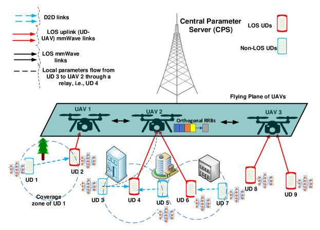
Figure 1: ATIN network with one CPS, $3$ UAVs, $9$ UDs, and a set of RRBs per each UAV. For instance, UDs $1$, $3$, $5$, and $7$ do not have direct LOS links to the UAVs. Thus, they transmit the trained local models to the UAVs via LOS UDs, e.g., UDs $2$, $4$, and $6$. UDs $8$ and $9$ can transmit their models directly to the UAVs via LOS mmWave links.

II-B Transmission Time Structure

The UAVs start local model aggregations after receiving the local trained models of the scheduled UDs across all the RRBs. Since different UDs $\mathcal{U}_{los}$ will have different transmission rates, they will have different transmission durations for uploading their trained parameters to the UAVs/RRBs. Let $s$ be the size of the UD’s local vector parameter (which is the same for the global model), expressed in bits. Note that the analysis in this subsection is for the transmission duration of one global iteration $t$. For simplicity, we represent $X$ as the number of elements in the set $\mathcal{X}$. The time required by the $u$-th UD, $u\in\mathcal{U}_{los}$, to reliably transmit its model update to the $k$-th selected UAV over the $b$-th RRB is then given by $T_{u}=\frac{s}{R^{u}_{k,b}}$. With this consideration, we can see that, given the number of participating UDs $U_{los}$, the transmission duration is $\max_{u\in\mathcal{U}_{los}}\{T_{u}\}=\max_{u\in\mathcal{U}_{los}}\frac{s}{R^{u}_{k,b}}$. When $U_{los}$ is large, $\max_{u\in\mathcal{U}_{los}}\{T_{u}\}$ can dramatically grow. The transmission duration is therefore constrained by the minimum rate of the scheduled UDs $\mathcal{U}_{los}$, i.e., $\min_{u\in\mathcal{U}_{los}}\{R^{u}_{k,b}\}$. Without the loss of generality, let us assume that UD $u\in\mathcal{U}_{los}$ has the minimum rate that is denoted by $R^{u}_{min}$. The corresponding transmission duration is $\frac{s}{R^{u}_{min}}$. The design of $R^{u}_{min}$ dominates the local models transmission duration from the UDs to the UAVs, thus it dominates the time duration of one FL global iteration. This is because the FL time consists of the local models transmission time and the learning computation time. Since the computation times of the UDs for local learning does not differ much, the FL time of one global iteration is dominated by $R^{u}_{min}$. Thus, $R^{u}_{min}$ can be adapted to include fewer or more UDs in the training process.

For the different transmission durations $\mathcal{U}_{los}$, some UDs will finish transmitting their local models before other UDs. Thus, high transmission rate UDs in $\mathcal{U}_{los}$ will have to wait to start a new iteration simultaneously with relatively good transmission rate UDs. We propose to efficiently exploit such waiting times to assist the UDs that have non-LOS channels to the UAVs. Define the portion of the time that not being used by $\bar{u}$-th UD (i.e., $\bar{u}\neq u,u\in\mathcal{U}_{los}$) at the $t$-th iteration is referred to as the idle time of the $\bar{u}$-th UD and denoted by $T^{\bar{u}}_{idle}$. This idle time can be expressed as $T^{\bar{u}}_{idle}=(\frac{s}{R^{\bar{u}}_{k,b}}-\frac{s}{R^{u}_{min}})$ seconds. Such idle time can be exploited by UDs $\bar{u}\in\mathcal{U}_{los}$ via D2D links if they ensure the complete transmission of the local parameters of the non-LOS UDs to the UAVs. More specifically, the idle time of the $\bar{u}$-th UD should be greater than or equal to the transmission duration of sending the local parameters from the $\hat{u}$-th non-LOS UD to the $\bar{u}$-th UD plus the time duration of forwarding the local parameters from the $\bar{u}$-th UD to the $k$-th UAV. Mathematically, it must satisfy $T^{\bar{u}}_{idle}\geq(\frac{s}{R^{\bar{u}}_{\hat{u}}}+\frac{s}{R^{\bar{u}}_{k,b}})$. From now on, we will use the term relay to UD $\bar{u}\neq u,\bar{u}\in\mathcal{U}_{los}$. In relay mode, each communication period is divided into two intervals corresponding to the non-LOS UD-relay phase (D2D communications) and relay-UAV phase (mmWave communication). The aforementioned transmission duration components of UDs and relays for one global iteration is shown in Fig. 2. Note that UDs can re-use the same frequency band and transmit simultaneously via D2D links.

When the $\hat{u}$-th UD does not have a LOS communication to any of the UAVs, it may choose the $\bar{u}$-th UD as its relay if the $\bar{u}$-th relay is located in the coverage zone of the $\hat{u}$-th UD. Let $\mathcal{U}_{\hat{u}}$ is the set of relays in the coverage zone of UD $\hat{u}$. Let $h^{\bar{u}}_{\hat{u}}$ denote the channel gain for the D2D link between the $\hat{u}$-th UD and the $\bar{u}$-th relay. Then, the achievable rate of D2D pair $(\hat{u},\bar{u})$ is given by $R^{\bar{u}}_{\hat{u}}=W\log_{2}(1+\frac{p|h^{\bar{u}}_{\hat{u}}|^{2}}{N_{0}}),\forall\bar{u}\in\mathcal{U}_{los},\hat{u}\in\mathcal{U}_{non}$. In relay mode, the transmission duration for sending the local parameter of the $\hat{u}$-th UD to the $k$-th UAV through relay $\bar{u}$ is $\mathtt{T}_{\hat{u}}=\frac{s}{R^{\bar{u}}_{\hat{u}}}+\frac{s}{R^{\bar{u}}_{k,b}}$, which should satisfy $\mathtt{T}_{\hat{u}}\leq T^{\bar{u}}_{idle}$.

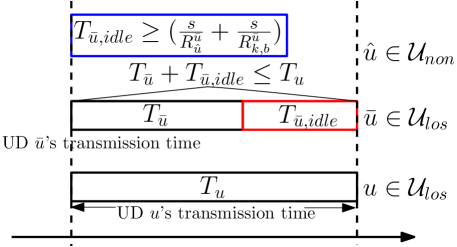
Figure 2: Transmission time structure for LOS UDs and non-LOS UDs for the $t$-th global iteration.

III FedMoD

III-A Federated Learning Process

In FL, each UD $u$ possesses a set of local training data, denoted as $\mathcal{D}_{u}$. The local loss function on the dataset of the $u$-th UD can be calculated as

$$F_{u}(\mathbf{w})=\frac{1}{|\mathcal{D}_{u}|}\sum_{(x_{i},y_{i})\in\mathcal{D}_{u}}f_{i}(\mathbf{w}),\forall u\in\mathcal{U},$$ (5)

where $x_{i}$ is the sample $i$’s input (e.g., image pixels) and $y_{i}$ is the sample $i$’s output (e.g., label of the image) and $f_{i}(\mathbf{w})$ is the loss function that measures the local training model error of the $i$-th data sample. The collection of data samples at the set of UDs that is associated with the $k$-th UAV is denoted as $\mathcal{\tilde{D}}_{k}$, and the training data at all the learning involved UDs, denoted as $\mathcal{U}_{inv}$, is denoted as $\mathcal{D}$. The ratios of data samples are defined as $\hat{m}_{u}=\frac{|\mathcal{D}_{u}|}{|\mathcal{\tilde{D}}_{k}|}$, $m_{u}=\frac{|\mathcal{D}_{u}|}{|\mathcal{D}|}$, and $\tilde{m}_{k}=\frac{|\mathcal{\tilde{D}}_{k}|}{|\mathcal{D}|}$, respectively. We define the loss function for the $k$-th UAV as the average local loss across the $k$-th cluster $\hat{F}(\mathbf{w})=\sum^{|\mathcal{U}_{k}|}_{u=1}\frac{|\mathcal{D}_{u}|}{|\mathcal{\tilde{D}}_{k}|}F_{u}(\mathbf{w})$. The global loss function $F(\mathbf{w})$ is then defined as the average loss across all the clusters $F(\mathbf{w})=\sum^{|\mathcal{U}_{inv}|}_{u=1}\frac{|\mathcal{D}_{u}|}{|\mathcal{D}|}F_{u}(\mathbf{w})$. The objective of the FL model training is to find the optimal model parameters $\mathbf{w}^{*}$ for $F(\mathbf{w})$ that is expressed as follows $\mathbf{w}^{*}=\arg\min_{\mathbf{w}}F(\mathbf{w})$. In this work, we propose FedMoD that involves three main procedures: 1) local model update at the UDs, 2) local model aggregation at the UAVs, and 3) model dissemination between the UAVs.

1) Local Model Update: Denote the model of the $u$-th UD at the $t$-th global iteration as $\mathbf{w}_{u}(t)$. This UD performs model updating based on its local dataset by using stochastic gradient descent (SGD) algorithm, which is expressed as follows

$$\mathbf{w}_{u}(t)=\mathbf{w}_{u}(t-1)-\lambda g(\mathbf{w}_{u}(t-1)),$$ (6)

where $\lambda$ is the learning rate and $g(\mathbf{w}_{u}(t-1))$ is the stochastic gradient computed on the dataset of the $u$-th UD.

2) Local Model Aggregation: After all the selected UDs completing their local model updates, they offload their model parameters over the available RRBs to the associated UAVs. A typical UAV $k$ aggregates the received models by computing a weighted sum as follows

$$\mathbf{\tilde{w}}_{k}(t)=\sum_{u\in\mathcal{U}_{k}}\hat{m}_{u}\mathbf{w}_{u}(t),\forall k\in\mathcal{K}.$$ (7)

3) Model Dissemination: Each UAV disseminates its local aggregated model to the one-hop neighboring UAVs. The model dissemination includes $l=1,2,\cdots,\alpha$ times of model dissemination until at least one UAV receives the local aggregated models of other UAVs, where $\alpha$ is the number of dissemination rounds. Specifically, at the $t$-th iteration, the $k$-th UAV aggregates the local models of its associated UDs as in (7).

At the beginning of the model dissemination step, the $k$-th UAV knows only $\mathbf{\tilde{w}}_{k}(t)$ and does not know the models of other UAVs’ models $\mathbf{\tilde{w}}_{j}(t),j\neq k,\forall j\in\mathcal{K}$. Consequently, at the $t$-th global iteration and $l$-th round, the $k$-th UAV has the following two sets:

• The Known local aggregated model: Represented by $\mathcal{H}^{l}_{k}(t)=\{\mathbf{\tilde{w}}_{k}(t)\}$.

• The Unknown local aggregated models: Represented by $\mathcal{W}^{l}_{k}(t)=\{\mathbf{\tilde{w}}_{j}(t),\mathbf{\tilde{w}}_{\tilde{j}}(t),\cdots,\mathbf{\tilde{w}}_{K}(t)\}$ and defined as the set of the local aggregated models of other UAVs.

These two sets are referred as the side information of the UAVs. For instance, at $l=\alpha$, the side information of the $k$-th UAV is $\mathcal{H}^{\alpha}_{k}(t)=\{\mathbf{\tilde{w}}_{k}(t),\mathbf{\tilde{w}}_{j}(t),\mathbf{\tilde{w}}_{\tilde{j}}(t),\cdots,\mathbf{\tilde{w}}_{K}(t)\}$ and $\mathcal{W}^{\alpha}_{k}(t)=\emptyset$. To achieve global model consensus, UAV $k$ needs to know the other UAVs’ models, i.e., $\mathcal{W}_{k}(t)$, so as to aggregate a global model for the whole network. To this end, we propose efficient model dissemination scheme that enables the UAVs to obtain their Unknown local aggregated models $\mathcal{W}_{k}(t),\forall k\in\mathcal{K},$ with minimum dissemination latency.

III-B Model Dissemination

To overcome the need of CPS for global aggregations or UAV coordination, an efficient distributed model dissemination method is developed. Note that all the associations of UAVs $\mathcal{K}_{k}$ can be computed locally at the $k$-th UAV since all the needed information (e.g., complex channel gains and the indices of the local aggregated models) are locally available. In particular, UAV $k\in\mathcal{K}$ knows the information of its neighboring UAVs only.

At each dissemination round, transmitting UAVs use the previously mentioned side information to perform XOR model encoding, while receiving UAVs need the stored models to obtain the Unknown ones. The entire process of receiving the Unknown models takes a small duration of time. According to the reception status feedback by each UAV, the UAVs distributively select the transmitting UAVs and their models to be transmitted to the receiving UAVs at each round $l$. The transmitted models can be one of the following two options for each receiving UAV $i$:

• Non-innovative model (NIM): A coded model is non-innovative for the receiving UAV $i$ if it does not contain any model that is not known to UAV $i$.

• Decodable model (DM): A coded model is decodable for the receiving UAV $i$ if it contains just one model that is not known to UAV $i$.

In order to represent the XOR coding opportunities among the models not known at each UAV, we introduce a FedMoD conflict graph. At round $l$, the FedMoD conflict graph is denoted by $\mathcal{G}(\mathcal{V}(l),\mathcal{E}(l))$, where $\mathcal{V}(l)$ refers to the set of vertices, $\mathcal{E}(l)$ refers to the set of encoding edges. Let $\mathcal{K}_{k}$ be the set of neighboring UAVs to the $k$-th UAV, and let $\mathcal{K}_{w}\subset\mathcal{K}$ be the set of UAVs that still wants some local aggregated models. Hence, the FedMoD graph is designed by generating all vertices for the $k$-th possible UAV transmitter that can provide some models to other UAVs, $\forall k\in\mathcal{K}$. The vertex set $\mathcal{V}(l)$ of the entire graph is the union of vertices of all possible transmitting UAVs. Consider, for now, generating the vertices of the $k$-th UAV. Note that the $k$-th UAV can exploit its previously received models $\mathcal{H}^{l}_{k}(t)$ to transmit an encoded/uncoded model to the set of requesting UAVs. Therefore, each vertex is generated for each model $m\in\mathcal{W}^{l}_{i}(t)\cap\mathcal{H}^{l}_{k}(t)$ that is requested by each UAV $i\in\mathcal{K}_{w}\cap\mathcal{K}_{k}$ and for each achievable rate of the $k$-th UAV $r\in\mathcal{R}_{k,i}=\{r\in\mathcal{R}_{k}|r\leq r_{k,i}\leavevmode\nobreak\ \text{and}\leavevmode\nobreak\ i\in\mathcal{K}_{w}\cap\mathcal{K}_{k}$}, where $\mathcal{R}_{k,i}$ is a set of achievable capacities between the $k$-th UAV and the $i$-th UAV, i.e., $\mathcal{R}_{k,i}\subset\mathcal{R}_{k}$. Accordingly, the $i$-th neighboring UAV in $\mathcal{K}_{k}$ can receive a model from the $k$-th UAV. Therefore, we generate $|\mathcal{R}_{k,i}|$ vertices for a requesting model $m\in\mathcal{H}^{l}_{k}(t)\cap\mathcal{W}^{l}_{i}(t),\forall i\in\mathcal{K}_{w}\cap\mathcal{K}_{k}$. A vertex $v^{k}_{i,m,r}\in\mathcal{V}(l)$ indicates the $k$-th UAV can transmit the $m$-th model to the $i$-th UAV with a rate $r$. We define the utility of vertex $v^{k}_{i,m,r}$ as

$$w(v^{k}_{i,m,r})=rN_{k},$$ (8)

where $N_{k}$ is the number of neighboring UAVs that can be served by the $k$-th UAV. This weight metric shows two potential benefits (i) $N_{k}$ represents that the $k$-th transmitting UAV is connected to many other UAVs that are requesting models in $\mathcal{H}^{t}_{k}(l)$; and (ii) $r$ provides a balance between the transmission rate and the number of scheduled UAVs.

Since UAVs communicate among them, their connectivity can be characterized by an undirected graph with sets of vertices and connections. All possible conflict connections between vertices (conflict edges between circles) in the FedMod conflict graph are provided as follows. Two vertices $v_{i,m,r}^{k}$ and $v_{i^{\prime},m^{\prime},r^{\prime}}^{k^{\prime}}$ are adjacent by a conflict edge in $\mathcal{G}$, if one of the following conflict conditions (CC) is true.

• CC1. (encoding conflict edge): ($k={k^{\prime}}$) and ($m\neq m^{\prime}$) and ($m,m^{\prime}$) $\notin\mathcal{H}^{l}_{k^{\prime}}(t)\times\mathcal{H}^{l}_{k}(t)$. A conflict edge between vertices in the same local FedMoD conflict graph is connected as long as their corresponding are not decodable to a set of scheduled UAVs.

• CC2. (rate conflict edge): ($k=k^{\prime}$) and ($k\neq k^{\prime}$) and ($r\neq r^{\prime}$). All adjacent vertices correspond to the same (or different) UAV $k$ should have the same achievable rate.

• CC3. (transmission conflict edge): ($k\neq k^{\prime}$) and ($i=i^{\prime}$). The same UAV cannot be scheduled to two different UAVs $k$ and $k^{\prime}$.

• CC4. (half-duplex conflict edge): ($k=i^{\prime}$) or ($k^{\prime}=i$). The same UAV can not transmit and receive in the same dissemination round.

To distributively disseminate the local aggregated models among the UAVs, we propose a graph theory method as follows. Let $\mathcal{S}_{k}$ represent the associations of the neighboring UAVs in the coverage zone of the $k$-th UAV, i.e., the associations of UAV $k$ to the set $\mathcal{K}_{k}$. Then, let the local FedMoD conflict graph $\mathcal{G}_{k}(\mathcal{S}_{k})\subset\mathcal{G}$ for an arbitrary UAV $k\in\mathcal{K}$ represent the set of associations $\mathcal{S}_{k}$. Our proposed distributed algorithm has two phases: i) the initial phase and ii) the conflict solution phase. In the initial phase, UAV $k\in\mathcal{K}$ constructs the local FedMoD conflict graph $\mathcal{G}_{k}(\mathcal{S}_{k})$ and selects its targeted neighboring UAVs using the maximum weight independent set (MWIS) search method [34, 35] that results in MWIS $\mathbf{S}_{k}$. Each UAV exchanges its scheduled UAVs with its neighbor UAV. Then the conflict solution phase starts. The UAV that is associated to multiple UAVs (UAV that is located at the overlapped regions of UAVs) is assigned to one UAV that offers the highest weight of scheduling that UAV. UAVs that do not offer the maximum weight cannot schedule that UAV, and therefore remove that UAV from their set of associated UAVs and vertices. We then design the new graph. We repeat this process until all the conflicting UAVs are scheduled to at most a single transmitting UAV. The details process of the algorithm for a single dissemination round are presented in Algorithm 1.

Data: $\mathcal{K}$, $\tilde{\mathbf{w}}_{k},\mathcal{H}^{0}_{k}(t),\mathcal{W}^{0}_{k}(t),\forall k\in\mathcal{K}$.

Initialize Phase:

Initialize: $\mathtt{K}=\emptyset$.

for all $k\in\mathcal{K}$ do

       Construct $\mathcal{G}_{k}(\mathcal{K}_{k})$ and calculate weight $w(v)$ using (8), $\forall v\in\mathcal{G}_{k}$.

       Find MWIS $\mathbf{S}_{k}$.

end for

Conflict Solution Phase: for $i=1,2,\cdots$ do

       Transmit $\hat{\mathbf{S}}_{k}=\{j\in\mathcal{K}_{k}\leavevmode\nobreak\ |\leavevmode\nobreak\ j\in\mathbf{S}_{k}\}$.

       Set $\mathtt{K}=\{j\in\mathcal{K}\leavevmode\nobreak\ |\leavevmode\nobreak\ \exists(k,k^{\prime})\in\mathcal{K}^{2},j\in\hat{\mathbf{S}}_{k}\cap\hat{\mathbf{S}}_{k^{\prime}}\}$.

       for all $j\in\mathtt{K}$ do

             Set $\hat{\mathcal{K}}(j)=\{k\in\mathcal{K}\leavevmode\nobreak\ |\leavevmode\nobreak\ j\in\hat{\mathbf{S}}_{k}\}$.

             for all $k\in\hat{\mathcal{K}}(j)$ do

                   Set $M_{kj}=\sum_{v\in\mathbf{S}_{k}}w(v)$ and $\mathcal{K}_{k}=\mathcal{K}_{k}\backslash\{j\}$.

                   Construct $\mathcal{G}_{k}(\mathcal{K}_{k})$ and compute $w(v)$ by (8) and solve $\tilde{\mathbf{S}}_{k}$ MWIS.

                   Set $\tilde{M}_{kj}=\sum_{v\in\tilde{\mathbf{S}}_{k}}w(v)$ and transmit $M_{kj}$ and $\tilde{M}_{kj}$.

             end for

            Set $k^{*}=\arg\max_{k\in\hat{\mathcal{K}}(j)}\left(M_{kj}+\sum_{k^{\prime}\in\hat{\mathcal{K}}(j),k\neq k^{\prime}}\tilde{M}_{k^{\prime}j}\right)$.

             Set $\mathcal{K}_{k^{*}}=\mathcal{K}_{k^{*}}\cup\{j\}$.

             for all $k\in\hat{\mathcal{K}}(j)\backslash\{k^{*}\}$ do

                   Set $\mathbf{S}_{k}=\tilde{\mathbf{S}}_{k}$.

             end for

            

       end for

      

end for

Result: $\mathbf{S}=\mathbf{S}_{k},\cdots$

Algorithm 1 Distributed UAV-UAV Scheduling for Model Dissemination

III-C Illustration of the Proposed Model Dissemination Method

For further illustration, we explain the dissemination method that is implemented at the UAVs through an example of the network topology of Fig. 3. Suppose that all the UAVs have already received the local models of their scheduled UDs and performed the local model averaging. Fig. 3 presents the side information status of each UAV at round $l=0$.

Figure 3: A simple example of $5$ UAVs with their arbitrary transmission rates and initial side information at round $l=0$.

Round 1: Since UAV $2$ has good reachability to many UAVs ($\mathcal{K}_{2}=\{1,4,3\}$), it transmits its model $\mathbf{\tilde{w}}_{2,0}$ to UAVs 1, 4, and 3 with a transmission rate of $r(l=1)=\min\{12,11,9\}=9$ Mbps (CC2 is satisfied). Note that UAV $5$ can not transmit to UAV $3$ according to CC3, i.e., UAV $3$ is already scheduled to the transmitting UAV $2$. When UAV $2$ finishes model transmission, the Known sets of the receiving UAVs is updated to $\mathcal{H}^{1}_{1}(t)=\{\mathbf{\tilde{w}}_{1},\mathbf{\tilde{w}}_{2}\}$, $\mathcal{H}^{1}_{3}(t)=\{\mathbf{\tilde{w}}_{3},\mathbf{\tilde{w}}_{2}\}$, and $\mathcal{H}^{1}_{4}(t)=\{\mathbf{\tilde{w}}_{4},\mathbf{\tilde{w}}_{2}\}$. Accordingly, their Unknown sets are: $\mathcal{W}^{1}_{1}(t)=\{\mathbf{\tilde{w}}_{3},\mathbf{\tilde{w}}_{4},\mathbf{\tilde{w}}_{5}\}$, $\mathcal{W}^{1}_{3}(t)=\{\mathbf{\tilde{w}}_{1},\mathbf{\tilde{w}}_{4},\mathbf{\tilde{w}}_{5}\}$, $\mathcal{W}^{1}_{4}(t)=\{\mathbf{\tilde{w}}_{1},\mathbf{\tilde{w}}_{3},\mathbf{\tilde{w}}_{5}\}$.

Round 2: Although UAV $2$ has good reachability to many UAVs, it would not be selected as a transmitting UAV at $l=2$. This is becasue UAV has already disseminated its side information to the neighboring UAVs, thus UAV $2$ does not have any vertex in the FedMoD conflict graph. In this case, UAVs $4$ and $5$ can simultaneously transmit models $\mathbf{\tilde{w}}_{4}$ and $\mathbf{\tilde{w}}_{5}$, respectively, to the receiving UAVs $\{1,2\}$ and $\{3\}$. When UAVs $4$ and $5$ finish models transmission, the Known sets of the receiving UAVs is updated to $\mathcal{H}^{2}_{1}(t)=\{\mathbf{\tilde{w}}_{1},\mathbf{\tilde{w}}_{2},\mathbf{\tilde{w}}_{4}\}$, $\mathcal{H}^{2}_{2}(t)=\{\mathbf{\tilde{w}}_{2},\mathbf{\tilde{w}}_{4}\}$, and $\mathcal{H}^{2}_{3}(t)=\{\mathbf{\tilde{w}}_{3},\mathbf{\tilde{w}}_{2},\mathbf{\tilde{w}}_{5}\}$. Clearly, UAVs $4$ and $5$ transmit their models to the corresponding UAVs with transmission rates of $r_{4}=\min\{13,15\}=13$ Mbps and $r_{5}=16$ Mbps, respectively. However, for simultaneous transmission and from CC2, all the vertices of the corresponding UAVs $\{1,2,3\}$ should have the same achievable rate. Thus, UAVs $4$ and $5$ adopt one transmission rate which is $r(l=2)=\min\{r_{4},r_{5}\}=13$ Mpbs.

Round 3: UAV $1$ transmits model $\mathbf{\tilde{w}}_{1}$ to the receiving UAVs $\{2,4\}$, and their Known sets are updated to $\mathcal{H}^{3}_{2}(t)=\{\mathbf{\tilde{w}}_{2},\mathbf{\tilde{w}}_{4},\mathbf{\tilde{w}}_{1}\}$, $\mathcal{H}^{3}_{4}(t)=\{\mathbf{\tilde{w}}_{4},\mathbf{\tilde{w}}_{2},\mathbf{\tilde{w}}_{1}\}$. UAV $1$ transmits its model to the corresponding UAVs with a transmission rate of $r(l=3)=\min\{10,14\}=10$ Mbps.

Round 4: Given the updated side information of the UAVs, UAV $3$ can encode models $\mathbf{\tilde{w}}_{5}$ and $\mathbf{\tilde{w}}_{2}$ into the encoded model $\mathbf{\tilde{w}}_{5}\oplus\mathbf{\tilde{w}}_{2}$ and broadcasts it to UAVs $2$ and $5$. Upon reception this encoded model, UAV $5$ uses the stored model $\mathbf{\tilde{w}}_{5}$ to complete model decoding $(\mathbf{\tilde{w}}_{5}\oplus\mathbf{\tilde{w}}_{2})\oplus\mathbf{\tilde{w}}_{5}=\mathbf{\tilde{w}}_{2}$. Similarly, UAV $5$ uses the stored model $\mathbf{\tilde{w}}_{2}$ to complete model decoding $(\mathbf{\tilde{w}}_{5}\oplus\mathbf{\tilde{w}}_{2})\oplus\mathbf{\tilde{w}}_{2}=\mathbf{\tilde{w}}_{5}$. The broadcasted model is thus decodable for both UAVs $5$ and $2$ and has been transmitted with a rate of $r(l=4)=\min\{11,15\}=11$ Mpbs. The Known sets of these receiving UAVs are as follows: $\mathcal{H}^{4}_{2}(t)=\{\mathbf{\tilde{w}}_{2},\mathbf{\tilde{w}}_{4},\mathbf{\tilde{w}}_{1},\mathbf{\tilde{w}}_{5}\}$ and $\mathcal{H}^{4}_{5}(t)=\{\mathbf{\tilde{w}}_{5},\mathbf{\tilde{w}}_{2}\}$.

Round 5: Given the updated side information of the UAVs at $l=4$, UAV $3$ transmits $\mathbf{\tilde{w}}_{3}$ to UAVs $2$ and $5$. Upon reception this model, UAV $2$ has obtained all the required models, i.e., $\mathcal{H}^{5}_{2}(t)=\{\mathbf{\tilde{w}}_{1},\mathbf{\tilde{w}}_{2},\mathbf{\tilde{w}}_{3},\mathbf{\tilde{w}}_{4},\mathbf{\tilde{w}}_{5}\}$ and $\mathcal{W}^{5}_{2}(t)=\{\emptyset\}$. The broadcasted model is transmitted with a rate of $r(l=5)=\min\{11,15\}=11$ Mpbs. Since UAV $2$ has all the local aggregated models of other UAVs, it can aggregate them all which results the global model at the $t$-th iteration:

$$\mathbf{\tilde{w}}(t)=\frac{1}{D}(\mathbf{\tilde{w}}_{1}+\mathbf{\tilde{w}}_{2}+\mathbf{\tilde{w}}_{3}+\mathbf{\tilde{w}}_{4}+\mathbf{\tilde{w}}_{5}).$$ (9)

Therefore, the global model $\mathbf{\tilde{w}}$ is broadcasted from UAV $2$ to UAVs $\{1,4,3\}$ with a rate of $\min\{12,11,9\}=9$ Mpbs. Next, UAV $3$ can send $\mathbf{\tilde{w}}$ to UAV $5$ with a rate of $15$ Mbps. Therefore, all the UAVs obtain the shared global model $\mathbf{\tilde{w}}$ and broadcast it to their scheduled UDs to initialize the next iteration $t+1$. Note that the transmission duration of these dissemination rounds is

$$T_{diss}=\underbrace{\frac{s}{9}}_{l=1}+\underbrace{\frac{s}{13}}_{l=2}+\underbrace{\frac{s}{10}}_{l=3}+\underbrace{\frac{s}{11}}_{l=4}+\underbrace{\frac{s}{11}}_{l=5}+\underbrace{\frac{s}{9}+\frac{s}{15}.}_{\mathbf{\tilde{w}}\leavevmode\nobreak\ \text{broadcasting}}$$ (10)

The size of a typical model is $s=9.098$ Kb [36, 13, 37], thus $T_{diss}=0.0059$ sec. Thanks to the efficient model dissemination proposed method that disseminates models from transmitting UAVs to the closest receiving UAVs with good connectivity, the dissemination delay is negligible.
Remark 1: In the fully connected model, each UAV can receive the local aggregated models of all UAVs in $K$ dissemination rounds, where each UAV takes a round for broadcasting its local aggregated model to other UAVs.

The steps of FedMoD that includes local model update, local aggregation at the UAVs, and model dissemination among the UAVs are summarized in Algorithm 2.

Data: Number of global iterations $T$, number of local iterations $T_{l}$

Initialize: $t=1$ and start with the same model for each UD $u$: $\mathbf{w}_{u}(t-1)$.

for $t=1,2,\cdots,T$ do

       for each UD $u\in\mathcal{U}_{inv}$ in parallel do

             Update the local model as $\mathbf{w}_{u}(t)$ according to (5).

       end for

      for each UAV $k\in\mathcal{K}$ in parallel do

             Receive the most updated model from the UDs in $\mathcal{U}_{k}$.

             Obtain $\mathbf{\tilde{w}}_{k}(t)$ by performing local model aggregation according to (7).

             for $l=1,2,\cdots,\alpha$ do

                   UAVs dissiminate their models among them as expalined in Section III-B and Algorithm 1.

                  

             end for

            

       end for

      Update $\mathbf{\tilde{w}}_{k}(t-1)=\mathbf{\tilde{w}}_{k}(t)=\mathbf{w}(t)$.

       Broadcast $\mathbf{w}(t)$ to the UDs in $\mathcal{U}_{k}$.

      Update $t=t+1$.

end for

Result: Final global model $\mathbf{w}$.

Algorithm 2 FedMoD Algorithm

III-D Convergence Analysis

In this sub-section, we prove the convergence of FedMoD. To facilitate the convergence rate analysis of the proposed scheme, we first provide the following assumptions. For all $u\in\mathcal{U}$, we assume:

1. The local loss function is $L$-smooth, i.e.,. This assumption implies that for some $L>0$, $\lVert\triangledown F_{u}(\mathbf{w}(t+1))-\triangledown F_{u}(\mathbf{w}(t))\rVert_{2}\leq L\lVert\mathbf{w}(t+1)-\mathbf{w}(t)\rVert_{2}$.

2. The mini-batch gradient is unbiased, i.e., $\mathbb{E}_{\mathcal{D}_{u}|\tilde{\mathbf{w}}}[f(\mathcal{D}_{u};\tilde{\mathbf{w}})]=\triangledown F_{u}(\tilde{\mathbf{w}}),$ and there exists $\sigma>0$ such that $\mathbb{E}_{\mathcal{D}_{u}|\tilde{\mathbf{w}}}\bigg{\lVert}[f(\mathcal{D}_{u};\tilde{\mathbf{w}})]-\triangledown F_{u}(\tilde{\mathbf{w}})\bigg{\lVert}^{2}_{2}\leq\sigma^{2}$.

3. For the degree of non-IIDness, we assume that there exists $\kappa>0$ such that $\lVert\triangledown F_{u}(\tilde{\mathbf{w}})-\triangledown F(\tilde{\mathbf{w}})\lVert_{2}\leq\kappa,$ where $\kappa$ measures the degree of data heterogeneity across all UDs.

In centralized FL, the global model at the CPS at each global iteration evolves according to the following expression [13]:

$$\mathbf{w}(t+1)=\mathbf{w}(t)-\lambda\mathbf{G}(t),$$ (11)

where $\mathbf{w}(t)=[\mathbf{w}_{u}(t)]_{u\in\mathcal{U}_{inv}}$ and $\mathbf{G}(t)=[g(\mathbf{w}_{u}(t))]_{u\in\mathcal{U}_{inv}}$. However, in FedMoD, the $k$-th UAV maintains a model updated based on the trained models of its scheduled UDs only and needs to aggregate the models of other UAVs using the model dissemination method as in Section III-B. Theretofore, each UAV has insufficient model averaging unless the model dissemination method is performed until all UAVs obtain the global model defined in (9), i.e., at $l=\alpha$. In other words, at $l=\alpha$, the global model of our proposed decentralized FL should be the one mentioned in (11). For convenience, we define $\mathbf{\tilde{u}}(t)=\sum_{u\in\mathcal{U}_{inv}}m_{u}\mathbf{w}_{u}(t)$, and consequently, $\mathbf{\tilde{u}}(t)=\mathbf{\tilde{w}}(t)\mathbf{m}$. By multiplying both sides of the evolution expression in (11) by $\mathbf{m}$, yielding the following expression

$$\mathbf{\tilde{u}}(t+1)=\mathbf{\tilde{u}}(t)-\lambda\mathbf{G}(t)\mathbf{m},$$ (12)

Following [25, 26] and leveraging the evolution expression of $\mathbf{\tilde{u}}(t)$ in (12), we bound the expected change of the local loss functions in consecutive iterations as follows.

Lemma 1.

The expected change of the global loss function in two consecutive iterations can be bounded as follows

$$\mathbb{E}[F(\mathbf{\tilde{u}}(t+1))]-\mathbb{E}[F(\mathbf{\tilde{u}}(t))]\leq\frac{-\lambda}{2}\mathbb{E}\lVert\triangledown F(\mathbf{\tilde{u}}(t))\lVert^{2}_{2}$$

$$+\frac{\lambda^{2}L}{2}\sum_{u=1}^{{U_{inv}}}m_{u}\sigma^{2}-\frac{\lambda}{2}(1-\lambda L)\tilde{Q}+\frac{\lambda L^{2}}{2}\mathbb{E}\bigg{\lVert}\mathbf{\tilde{w}}(t)(\mathbf{I}-\mathbf{M})\bigg{\lVert}^{2}_{\mathbf{M}},$$ (13)

where $\tilde{Q}=\mathbb{E}\bigg{[}\bigg{\lVert}\sum_{u=1}^{U_{inv}}m_{u}\triangledown F_{u}(\mathbf{w}_{u}(t))\bigg{\lVert}^{2}_{2}\bigg{]}$, $\mathbf{M}=\mathbf{m}\mathbf{I}^{T}$, and $\lVert\mathbf{X}\lVert_{\mathbf{M}}=\sum_{i=1}^{M}\sum_{j=1}^{N}m_{i,j}|x_{i,j}|^{2}$ is the weighted Frobenius norm of an $M\times N$ matrix $\mathbf{X}$.

For proof, please refer to Appendix A.

Notice that $\mathbf{\tilde{w}}(t)$ deviates from the desired global model due to the partial connectivity of the UAVs that results in the last term in the right-hand side (RHS) of (1). However, through the model dissemination method and at $l=\alpha$, FedMoD ensures that each UAV can aggregate the models of the whole network at each global iteration before proceeding to the next iteration. Thus, such deviation is eliminated.

Due to the model dissemination among the UAVs, there is a dissemination gap that is denoted by the dissemination gap between the $k$-th and $j$-th UAVs as $\delta_{j,k}(t)$, which is the number of dissemination steps that the local aggregated model of the $j$-th UAV needs to be transmitted to the $k$-th UAV. For illustration, consider the example in Fig. 3, the highest dissemination gap is the one between UAVs $5$ and $1$ which is $3$. Thus, $\delta_{5,1}(t)=3$. The maximum dissemination gap of UAV $k$ is $\delta_{k}(t)=\max_{j\in\mathcal{K}}\{\delta_{j,k}(t)\}$. Therefore, a larger value of $\delta_{j,k}(t)$ implies that the model of each UAV needs more dissemination step to be globally converged. The following remark shows that $\delta_{k}(t)$ is upper bounded throughout the whole training process.
Remark 2: There exists a constant $\delta_{max}$ such that $\delta_{k}(t)\leq\delta_{max}$, $\forall t\in T,k\in\mathcal{K}$. At any iteration $t$, the dissemination gap of the farthest UAV (i.e., the UAV at the network edge), $\delta_{max}=\alpha$ gives a maximal value for the steps that the models of other UAVs have been disseminated to UAV $k$.

Given the aforementioned analysis, we are now ready to prove the convergence of FedMoD.

Theorem 1.

If the learning rate $\lambda$ satisfies $1-\lambda L\geq 0,1-2\lambda^{2}L^{2}>0$, we have

$$\small\mathbb{E}[\lVert\triangledown F(\tilde{\mathbf{u}})(t)\lVert^{2}_{2}]\leq\frac{2\{\mathbb{E}[F(\tilde{\mathbf{u}})(0)-F(\tilde{\mathbf{u}})(T)]\}}{\delta}+\lambda L\sum_{u=1}^{U_{inv}}m_{u}\sigma^{2}$$ (14)

Proof.

From (1), we have

$$\frac{\lambda}{2}\mathbb{E}\lVert\triangledown F(\mathbf{\tilde{u}}(t))\lVert^{2}_{2} \leq\mathbb{E}[F(\mathbf{\tilde{u}}(t))]-\mathbb{E}[F(\mathbf{\tilde{u}}(t+1))]$$

$$+\frac{\lambda^{2}L}{2}\sum_{u=1}^{U_{inv}}m_{u}\sigma^{2}-\frac{\lambda}{2}(1-\lambda L)\tilde{Q}.$$ (15)

$$\mathbb{E}\lVert\triangledown F(\mathbf{\tilde{u}}(t))\lVert^{2} \leq\frac{2\{\mathbb{E}[F(\mathbf{\tilde{u}}(t))]-\mathbb{E}[F(\mathbf{\tilde{u}}(t+1))]\}}{\lambda}$$

$$+\lambda L\sum_{i=1}^{U_{inv}}m_{u}\sigma^{2}-(1-\lambda L)\tilde{Q}$$ (16)

Since $1-\lambda L\geq 0$ from Theorem 1, the third term in the RHS of (III-D) is eliminated, thus we have

$$\mathbb{E}[\lVert\triangledown F(\tilde{\mathbf{u}})(t)\lVert^{2}]\leq\frac{2\{\mathbb{E}[F(\tilde{\mathbf{u}})(0)-F(\tilde{\mathbf{u}})(T)]\}}{\lambda}+\lambda L\sum_{u=1}^{U_{inv}}m_{u}\sigma^{2}$$ (17)

∎

IV FedMoD: Modeling and Problem Formulation

IV-A FL Time and Energy Consumption

1) FL Time: The constrained FL time at each global iteration consists of both computation and wireless transmission time that is explained below.

The wireless transmission time consists of (1) the uplink transmission time for transmitting the local updates from the UDs to the associated UAVs $\mathcal{K}$. This transmission time is already discussed in Section II-C and represented by $T_{u}$. (2) The transmission time for disseminating the local aggregated models among the UAVs. The model dissemination time among all the UAVs is $T_{diss}$ as given in (10). (3) The downlink transmission time for transmitting the local aggregated models from the UAVs to the scheduled UDs $\mathcal{U}$. The downlink transmission time for UAV $k$ can be expressed $T^{do}_{k}=\frac{s}{R_{k}}$. On the other hand, the computation time for local learning at the $u$-th UD is expressed as $T^{comp}_{u}=T_{l}\frac{Q_{u}D_{u}}{f_{u}},$ where $T_{l}$ is the number of local iterations to reach the local accuracy $\epsilon_{l}$ in the $u$-th UD, $Q_{u}$ as the number of CPU cycles to process one data sample, and $f_{u}$ is the computational frequency of the CPU in the $u$-th UD (in cycles per second).

By combining the aforementioned components, the FL time $\tau_{k}$ at the $k$-th UAV can be calculated as

$$\tau_{k} =\max_{u\in\mathcal{U}_{k}}T^{comp}_{u}+\max_{u\in\mathcal{U}_{k}}T^{com}_{u}+T^{do}_{k}$$

$$=\max_{u\in\mathcal{U}_{k}}\left\{T_{l}\frac{Q_{u}D_{n}}{f_{u}}\right\}+\max_{u\in\mathcal{N}_{k}}\left\{\frac{s}{R_{k,b}^{u}}\right\}+\frac{s}{R_{k}}.$$ (18)

Therefore, the total FL time over all global iterations $T$ is $\tau=T(\max_{k\in\mathcal{K}}(\tau_{k})+T_{diss})$, which should be no more than the maximum FL time threshold $T_{\text{max}}$. This constraint, over all global iterations $T$, is expressed as

$$\tau=T\bigg{(}\underbrace{\max_{u\in\mathcal{N}}\left\{T_{l}\frac{Q_{n}D_{u}}{f_{u}}\right\}}_{\text{local learning}}+\underbrace{T_{u}}_{\text{uplink transmission}}+\underbrace{\max_{k\in\mathcal{K}}\left\{\frac{s}{R_{k}}\right\}}_{\text{downlink transmission}}$$

$$+\underbrace{T_{diss}}_{\text{dissemination duration}}\bigg{)}\leq T_{\text{max}}.$$ (19)

2) Energy Consumption: The system’s energy is consumed for local model training at the UDs, wireless models transmission, and UAVs’ hovering in the air.

1) Local computation: The well-known energy consumption model for the local computation is considered, where the energy consumption of the $u$-th UD to process a single CPU cycle is $\alpha f^{2}_{u}$, and $\alpha$ is a constant related to the switched capacitance [38, 39]. Thus, the energy consumption of the $u$-th UD for local computation is $E^{comp}_{u}=T_{loc}C_{u}D_{u}\alpha f^{2}_{u}.$

2) Wireless models transmission: The energy consumption to transmit the local model parameters to the associated UAVs can be denoted by $E^{com}_{u}$ and calculated as $E^{com}_{u}=P_{u}T^{com}_{u}$. Then, the total energy consumption $E_{u}$ at the $u$-th UD is $E_{u}=E^{comp}_{u}+E^{com}_{u}$. In a similar manner, the consumed energy for transmitting the local aggregated models back to the associated UDs can be denoted by $E^{com}_{k}$ and calculated as $E^{com}_{k}=PT^{com}_{k}$.

3) UAV’s hovering energy: UAVs need to remain stationary in the air, thus most of UAV’s energy is consumed for hovering. The UAV’s hovering power is expressed as [40] $p^{hov}=\sqrt{\frac{(mg)^{3}}{2\pi r_{p}^{2}n_{p}\rho}},$ where $m$ is UAV’s weight, $g$ is the gravitational acceleration of the earth, $r_{p}$ is propellers’ radius, $n_{p}$ is the number of propellers, and $\rho$ is the air density. In general, these parameters of all the UAVs are the same. The hovering time of the $k$-th UAV in each global iteration depends on $\tau$. Hence, the hovering energy of the $k$-th UAV can be calculated as $E^{hov}_{k}=p^{hov}\tau^{t}$. In summary, the overall energy consumption of the $k$-th UAV and the $u$-th UD, respectively, are

$$E_{k}=T\left\{E^{hov}_{l}+E^{com}_{l}\right\},E_{u}=T\left\{E^{comp}_{u}+E^{com}_{u}\right\}.$$ (20)

IV-B Problem Formulation

Given the ATIN and its FL time and energy components, our next step is to formulate the energy consumption minimization problem that involves the joint optimization of two sub-problems, namely UAV-LOS UD clustering and D2D scheduling sub-problems. To minimize the energy consumption at each global iteration, we need to develop a framework that decides: i) the UAV-UD clustering; ii) the adopted transmission rate of the UDs $\mathcal{U}_{los}$ to transmit their local models to the set of UAVs/RRBs; and iii) the set of D2D transmitters (relays) that helping the non-LOS UDs to transmit their local models to the set of UAVs $\mathcal{K}$. As such, the local models are delivered to all UAVs with minimum duration time, thus minimum energy consumption for UAV’s hovering and UD’s wireless transmission. Therefore, the energy consumption minimization problem in the ATIN can be formulated as follows.

$$\text{P0:}\min_{\begin{subarray}{c}R^{u}_{min},\mathcal{U}_{los},\mathcal{U}_{non}\end{subarray}}\sum_{k\in\mathcal{K}}E_{k}+\sum_{u\in\mathcal{U}}E_{u}$$

$$\rm s.t.\begin{cases}\text{C1:}\hskip 5.69046pt\mathcal{U}_{k,los}\cap\mathcal{U}_{k^{\prime},los}=\emptyset,\forall(k,k^{\prime})\in\mathcal{K},\\ \text{C2:}\hskip 5.69046pt\mathcal{U}_{k,los}\cap\mathcal{U}_{u^{\prime},los}=\emptyset,\forall k\in\mathcal{K},\\ \text{C3:}\hskip 5.69046pt\mathcal{U}_{u,los}\cap\mathcal{U}_{u^{\prime\prime},los}=\emptyset,\\ \text{C4:}\hskip 5.69046ptR^{u}_{k,b}\geq R_{0},(u,k,b)\in(\mathcal{U},\mathcal{K},\mathcal{B}),\\ \text{C5:}\hskip 5.69046pt\mathtt{T}_{\hat{u}}\leq T_{u},u\in\mathcal{U}_{los},\\ \text{C6:}\hskip 5.69046ptT^{\bar{u}}_{idle}\geq(\frac{s}{R^{\bar{u}}_{\hat{u}}}+\frac{s}{R^{\bar{u}}_{k,b}}),\bar{u}\in\mathcal{U}_{los},\hat{u}\in\mathcal{U}_{non},\\ \text{C7:}\hskip 5.69046pt\tau\leq T_{\text{max}}.\end{cases}$$

The constraints are explained as follows. Constraint C1 states that the set of scheduled UDs to the UAVs are disjoint, i.e., each UD must be scheduled to only one UAV. Constraints C2 and C3 make sure that each UD can be scheduled to only one relay and no user can be scheduled to a relay and UAV at the same time instant. Constraint C4 is on the coverage threshold of each UAV. Constraint C5 ensures that the local parameters of UD $\hat{u}$ has to be delivered to UAV $k$ via relay $\bar{u}$ within $\frac{s}{R^{u}_{min}}$, i.e., $\mathtt{T}_{\hat{u}}=\frac{s}{R^{\bar{u}}_{\hat{u}}}+\frac{s}{R^{\bar{u}}_{k,b}}\leq\frac{s}{R^{u}_{min}}$. Constraint C6 ensures that the idle time of UD $\bar{u}$ is long enough for transmitting the local parameters of UD $\hat{u}$ to UAV $k$. Constraint C7 is for the FL time threshold $T_{max}$. We can readily show that problem P0 is NP-hard. However, by analyzing the problem, we can decompose it into two sub-problems and solve them individually and efficiently.

IV-C Problem Decomposition

First, we focus on minimizing the energy consumption via efficient RRM scheduling of UDs $\mathcal{U}_{los}$ to the UAVs/RRBs. In particular, we can get the possible minimum transmission duration of UD $u\in\mathcal{U}_{los}$ by jointly optimizing the UD scheduling and rate adaptation in $\mathcal{U}_{los}$. The mathematical formulation for minimizing the energy consumption via minimizing the transmission durations for UDs-UAVs/RRBs transmissions can be expressed as

$$\text{P1:}\min_{\begin{subarray}{c}R^{u}_{min},\mathcal{U}_{los}\end{subarray}}\sum_{k\in\mathcal{K}}E_{k}+\sum_{u\in\mathcal{U}}E_{u}$$

$$\rm s.t.\begin{cases}(\text{C1}),\hskip 5.69046pt(\text{C4}),\hskip 5.69046pt(\text{C5}),\hskip 5.69046pt(\text{C7}).\end{cases}$$

Note that this sub-problem contains UD-UAV/RRB scheduling and an efficient solution will be developed in Section IV-B.

After obtaining the possible transmission duration from UD-UAV transmissions, denoted by $T_{u}$ of the $u$-th UD ($u\in\mathcal{U}_{los}$), by solving P1, we can now formulate the second sub-problem. In particular, we can minimize the energy consumption of non-LOS UDs $\mathcal{U}_{non}$ that are not been scheduled to the UAVs within $T_{u}$ by using D2D communications via relaying mode. For this, UDs being scheduled to the UAVs from sub-problem P1 can be exploited to work as relays and schedule non-LOS UDs on D2D links within their idle times. Therefore, the second sub-problem of minimizing the energy consumption of unscheduled UDs to be scheduled on D2D links via relaying mode can be expressed as P2 as follows

$$\text{P2:}\min_{\begin{subarray}{c}\mathcal{U}_{non}\end{subarray}}\sum_{k\in\mathcal{K}}E_{k}+\sum_{u\in\mathcal{U}}E_{u}$$

$$\rm s.t.\begin{cases}(\text{C2}),\hskip 5.69046pt(\text{C3}),\hskip 5.69046pt(\text{C5}),\hskip 5.69046pt(\text{C6}),\text{C8:}\hskip 5.69046pt\mathcal{N}_{non}\in\mathcal{P}(\mathcal{U}\backslash\mathcal{N}_{los}).\\ \end{cases}$$

Constraint C8 states that the set of relays is constrained only on the UDs that are not been scheduled to the UAVs. It can be easily observed that P2 is a D2D scheduling problem that considers selection of relays and their non-LOS scheduled UDs.

V FedMoD: Proposed Solution

V-A Solution to Subproblem P1: UAV-UD Clustering

Let $\mathcal{A}$ denote the set of all possible associations between UAVs, RRBs, and LOS UDs, i.e., $\mathcal{A}=\mathcal{K}\times\mathcal{Z}\times\mathcal{U}_{los}$. For instance, one possible association $a$ in $\mathcal{A}$ is $(k,z,u)$ which represents UAV $k$, RRB $z$, and UD $u$. Let the conflict clustering graph in the network is denoted by $\mathcal{G}(\mathcal{V},\mathcal{E})$ wherein $\mathcal{V}$ and $\mathcal{E}$ are the sets of vertices and edges of $\mathcal{G}$, respectively. A typical vertex in $\mathcal{G}$ represents an association in $\mathcal{A}$, and each edge between two different vertices represents a conflict connection between the two corresponding associations of the vertices according to C1 in P1. Therefore, we construct the conflict clustering graph by generating a vertex $v\in\mathcal{V}$ associated with $a\in\mathcal{A}$ for UDs who have enough energy for performing learning and wireless transmissions. To select the UD-UAV/RRB scheduling that provides a minimum energy consumption while ensures C4 and C7 in P1, a weight $w(v)$ is assigned to each vertex $v\in\mathcal{V}$. For simplicity, we define the weight of vertex $v^{z}_{k,u}$ as $w(v^{z}_{k,u})=E^{comp}_{u}+E^{com}_{u}$. Vertices $v^{z}_{k,u}$ and $v^{z^{\prime}}_{k^{\prime},u^{\prime}}$ are conflicting vertices that will be connected by an edge in $\mathcal{E}$ if one of the below connectivity conditions (CC) is satisfied:

• CC1: ($u=u^{\prime}$ and $z=z^{\prime}$ or $k=k^{\prime}$). CC1 states that the same user $u$ is in both vertices $v^{z}_{k,u}$ and $v^{z^{\prime}}_{k^{\prime},u^{\prime}}$.

• CC2: ($z=z^{\prime}$ and $u\neq u^{\prime}$). CC2 implies that the same RRB is in both vertices $v^{z}_{k,u}$ and $v^{z^{\prime}}_{k,u^{\prime}}$.

Clearly, CC1 and CC2 correspond to a violation of the constraint C1 of P1 where two vertices are conflicting if: (i) the UD is associated with two different UAVs and(or) two different RRBs; or (ii) the RRB is associated with more than one UD. With the designed conflict clustering graph, $\text{P}1$ is similar to MWIS problems in several aspects. In MWIS, two vertices should be non-adjacent in the graph (conditions CC1 and CC2 in Section V-B), and similarly, in P1, same local learning user cannot be scheduled to two different UAVs or two different RRBs (i.e., C1). Moreover, the objective of problem P1 is to minimize the energy consumption, and similarly, the goal of MWIS is to select a number of vertices that have small weights. Therefore, the following theorem characterizes the solution to the energy consumption minimization problem P2 in an ATIN.
Theorem 2. The solution to problem P1 is equivalent to the minimum independent set weighting-search method, in which the weight of each vertex $v$ corresponding to UD $u$ is

$$w(v)=E^{comp}_{u}+E^{com}_{u}.$$ (24)

Finding the minimum weight independent set $\Gamma^{*}$ among all other minimal sets in $\mathcal{G}$ graph is explained as follows. First, we select vertex $v_{i}\in\mathcal{V},(i=1,2,\cdots,)$ that has the minimum weight $w(v^{*}_{i})$ and add it to $\Gamma^{*}$ (at this point $\Gamma^{*}=\{v^{*}_{i}\}$). Then, the subgraph $\mathcal{G}(\Gamma^{*})$, which consists of vertices in graph $\mathcal{G}$ that are not adjacent to vertex $v^{*}_{i}$, is extracted and considered for the next vertex selection process. Second, we select a new minimum weight vertex $v^{*}_{i^{\prime}}$ (i.e., $v^{*}_{i^{\prime}}$ should be in the corresponding set of $v^{*}_{i}$) from subgraph $\mathcal{G}(\Gamma^{*})$. Now, $\Gamma^{*}=\{v^{*}_{i},v^{*}_{i^{\prime}}\}$. We repeat this process until no further vertex is not adjacent to all vertices in $\Gamma^{*}$. The selected $\mathtt{C}$ contains at most $ZK$ vertices. Essentially, any possible solution $\Gamma^{*}=\{v^{*}_{1},v^{*}_{2},\cdots,v^{*}_{ZK}\}$ to P1 represents a feasible UD-UAV/RRB scheduling.

V-B Solution to Subproblem P2: D2D Graph Construction

In this subsection, our main focus is to schedule the non-LOS UDs to the LOS UDs (relays) over their idle times so as the local models of those non-LOS UDs can be forwarded to the UAVs. Since non-LOS UDs communicate with their respective relays over D2D links, the D2D connectivity can be characterized by an undirected graph $\mathcal{G}(\mathcal{V},\mathcal{E})$ with $\mathcal{V}$ denoting the set of vertices and $\mathcal{E}$ the set of edges. We construct a new D2D conflict graph that considers all possible conflicts for scheduling non-LOS UDs on D2D links, such as transmission and half-duplex conflicts. This leads to feasible transmissions from the potential D2D transmitters $|\mathcal{U}_{\text{non,tra}}|$.

Recall $\mathcal{U}_{\text{non}}$ is the set of non-LOS UDs, i.e., $\mathcal{U}_{\text{non}}=\mathcal{U}\backslash\mathcal{U}_{los}$, and let $\mathcal{U}_{\text{relay}}=\mathcal{U}_{\text{los}}\backslash\{u\}$ denote the set of relays that can use their idle times to help the non-LOS UDs. Hence, the D2D conflict graph is designed by generating all vertices for $\bar{u}$-th possible relay, $\forall\bar{u}\in\mathcal{U}_{\text{relay}}$. The vertex set $\mathcal{V}$ of the entire graph is the union of vertices of all users. Consider, for now, generating the vertices of the $\bar{u}$-th relay. Note that $\bar{u}$-th relay can help one non-LOS UD as long as it is in the coverage zone is capable of delivering the local model to the scheduled UAV within its idle time. Therefore, each vertex is generated for each single non-LoS UD that is located in the coverage zone of the $\bar{u}$-th relay and $\mathtt{T}_{\hat{u}}\leq T^{\bar{u}}_{idle}$. Accordingly, $i$-th non-LOS UD in the coverage zone $\mathcal{Z}_{\bar{u}}$ can transmit its model to the $\bar{u}$-th relay. Therefore, we generate $|\mathcal{Z}_{\bar{u}}|$ vertices for the $\bar{u}$-th relay.

All possible conflict connections between vertices (conflict edges between circles) in the D2D conflict graph are provided as follows. Two vertices $v_{i}^{\bar{u}}$ and $v_{i^{\prime}}^{u^{\prime}}$ are adjacent by a conflict edge in $\mathcal{G}_{\text{d2d}}$, if one of the following conflict conditions is true: (i) ($\bar{u}\neq u^{\prime}$) and ($i=i^{\prime}$). The same non-LoS UD cannot be scheduled to two different helpers $\bar{u}$ and $u^{\prime}$. (ii) ($i\neq i^{\prime}$) and ($\bar{u}=u^{\prime}$). Tow different non-LoS UDs can not be scheduled to the same relay. These two conditions represent C3 in P2, where each non-LoS UD must be assigned to one relay and the same relay cannot accommodate more than one non-LoS UD. Given the aforementioned designed D2D conflict graph, the following theorem reformulates the subproblem P3.
Theorem 3. The subproblem of scheduling non-LOS UDs on D2D links in $P2$ is equivalently represented by the MWIS selection among all the maximal sets in the $\mathcal{G}_{\text{d2d}}$ graph, where the weight $\psi(v_{i}^{\bar{u}})$ of each vertex $v_{i}^{\bar{u}}$ is given by $\psi(v_{i}^{\bar{u}})=r.$

VI Numerical Results

For our simulations, a circular network area having a radius of $400$ meter (m) is considered. The height of the CPS is $10$ m [40]. Unless specified otherwise, we divide the considered circular network area into $5$ target locations. As mentioned in the system model, each target location is assigned to one UAV where the locations of the UAVs are randomly distributed in the flying plane with altitude of $100$ m. The users are placed randomly in the area. In addition, $U$ users are connected to the UAVs through orthogonal RRBs for uplink local model transmissions. The bandwidth of each RRB is $2$ MHz. The UAV communicates with the neighboring UAVs via high-speed mmWave communication links [31, 25].

Our proposed FedMod scheme is evaluated on the MNIST and CIFAR-10 datasets, which are well-known benchmark datasets for image classification tasks. Each image is one of $10$ categories. We divide the dataset into the UDs’ local data $\mathcal{D}_{u}$ with non-i.i.d. data heterogeneity, where each local dataset contains datapoints from two of the $10$ labels. In each case, $\mathcal{D}_{u}$ is selected randomly from the full dataset of labels assigned to $u$-th UD. We also assume non-iid-clustering, where the maximum number of assigned classes for each cluster is $6$ classes. For ML models, we use a deep neural network with $3$ convolutional layers and $1$ fully connected layer. The total number of trainable parameters for MNIST is $9,098$ and for CIFAR-10 is $21,840$. We simulate an FedMod system with $30$ UDs (for CIFAR-10) and $20$ UDs (for MNIST) and $5$ UAVs each with $7$ orthogonal RRBs. In our experiments, we consider a network topology that is illustrated in Fig. 3 unless otherwise specified. The remaining simulation parameters are summarized in TABLE I and selected based on [13, 40, 42, 34, 41]. To showcase the effectiveness of FedMoD in terms of learning accuracy and energy consumption, we consider the Star-based FL and HFL schemes.

TABLE I: Simulation Parameters

Parameter	Value
Carrier frequency, $f$	$1$ GHz [40]
Speed of light, $c$	$3\times 10^{8}$ m/s
Propagation parameters, $a$ and $b$	$9.6$ and $0.28$ [40]
Attenuation factors, $\psi^{LoS}$ and $\psi^{nLoS}$	$1$ dB and $20$ dB [40]
UAV’s and UD’s transmit maximum powers, $P$, $p$	$1$ and $3$ Watt [40]
Transmit power of the CPS	$5$ Watt
Noise PSD, $N_{0}$	-$174$ dBm/Hz
Local and aggregated parameters size, $s$	$9.1$ KB
UD processing density, $C_{u}$	$[400-600]$
UD computation frequency, $f_{u}$	$[0.0003-1]$ G cycles/s
CPU architecture based parameter, $\alpha$	$10^{-28}$
FL time threshold $T_{max}$	$1$ Second
Number of data samples, $S_{u}$	$200$

We show the training accuracy with respect to number of iterations for both the MNIST and CIFAR-10 datasets with different model dissemination rounds $\alpha$ in Fig. 4. Specially, in Figs. 4(a) and 4(b), we show the accuracy performance of our proposed FedMoD scheme with full dissemination against the centralized FL schemes. Particularly, in the considered star-based and HFL schemes, the CPS can receive the local trained models from the UDs, where each scheduled UD transmits its trained model directly to the CPS (in case of star-based FL) or through UAVs (in case of HFL). Thus, the CPS can aggregate all the local models of all the scheduled UDs. In the considered decentralized FedMoD, before the dissemination rounds starts, each UAV has aggregated the trained local models of the scheduled UDs in its cluster only. However, with the novel dissemination FedMoD method, each UAV shares its aggregated models with the neighboring UAVs using one hop transmission. Thus, at each dissemination round, UAVs build their side information (Known models and Unknown models) until they receive all the Unknown models. Thus, the UAVs have full knowledge about the global model of the system at each global iteration. Thanks to the efficient FedMoD dissemination method, the accuracy of the proposed FedMoD scheme is almost the same as the centralized FL schemes. Such efficient communications among UAVs accelerate the learning progress, thereby FedMoD model reaches an accuracy of ($0.945$, $0.668$ for MNIST and CIFAR-10) with around $200$ and $300$ global iterations, respectively, as compared to the accuracy of ($0.955$, $0.944$ for MNIST) and ($0.665$, $0.668$ for CIFAR-10) for star-based and HFL schemes, respectively. It is important to note that although our proposed overcomes the struggling UD issue of the star-based scheme and the two-hop transmission of the HFL, it needs a few rounds of model dissemination. However, the effective coding scheme of the models minimizes the number of dissemination rounds. In addition, due to the high communication links between the UAVs, the dissemination delay is negligible which does not affect the FL time.

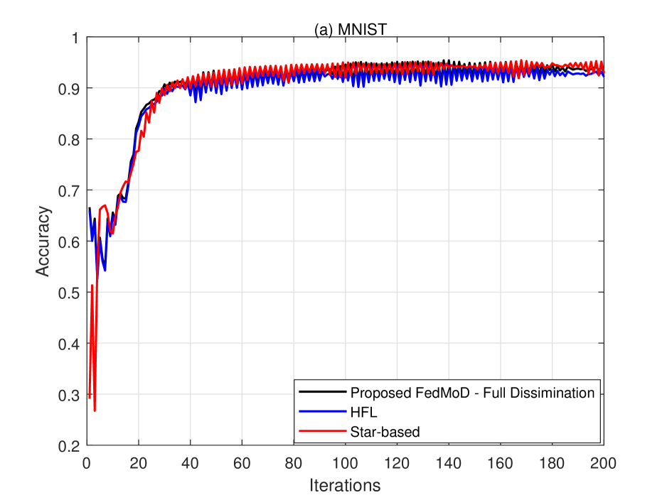
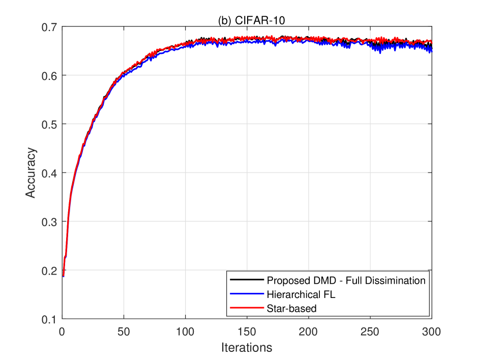
Figure 4: Performance comparison between FedMoD and baseline schemes for MNIST and CIFAR-10: Accuracy vs. number of iterations.

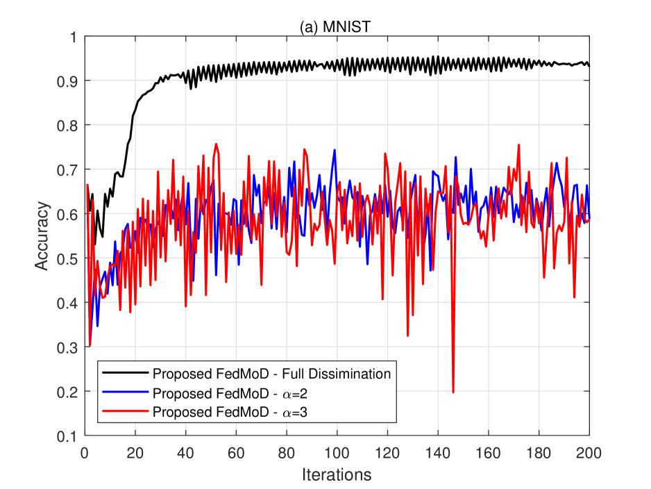
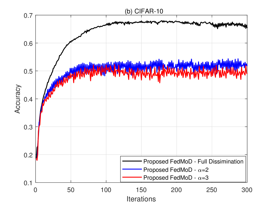
Figure 5: Performance comparison of FedMoD for MNIST and CIFAR-10 with different $\alpha$.

In Figs. 5(a) and 5(b), we further study the impact of the number of dissemination rounds $\alpha$ on the convergence rate of the proposed FedMoD scheme for both the MNIST and CIFAR-10 datasets. For both figures, we consider the following three proposed schemes: (i) FedMoD scheme-full dissemination where UAVs perform full model dissemination at each global iteration, (ii) FedMoD scheme - $\alpha=2$ where partially dissemination is performed and after each $2$ complete global iterations, we perform full dissemination, and (iii) FedMoD scheme - $\alpha=3$ where partially dissemination is performed and after each $3$ complete global iterations, a full dissemination is performed. From Figs. 5(a) and 5(b), we observe that a partial dissemination with less frequent full dissemination leads to a lower training accuracy within a given number of training iterations. Specifically, the accuracy performance for full dissemination, $\alpha=2$ and $3$ schemes is $0.966,0.66,0.75$ for MNIST and $0.668,0.52,0.59$ for CIFAR-10, respectively. Infrequent inter-cluster UAV dissemination also leads to un-stable convergence since the UAVs do not frequently aggregate all the local trained models of the UDs.

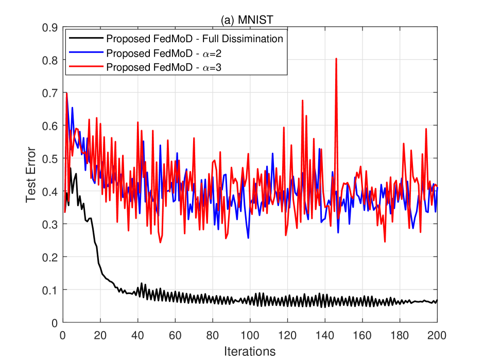
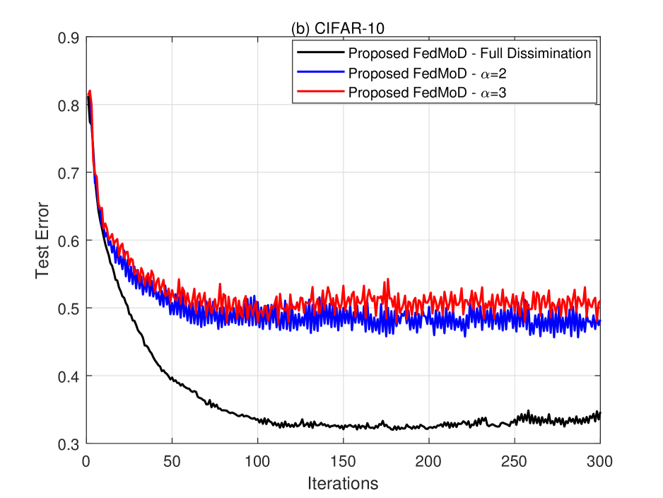
Figure 6: Test error of FedMoD for MNIST and CIFAR-10 with different $\alpha$.

In Figs. 6(a) and 6(b), we show the test error with respect to number of iterations for both the MNIST and CIFAR-10 datasets with different model dissemination rounds $\alpha$. It can be observed that, the test error of the proposed FedMod model drops rapidly at the early stage of the training process, and converges at around $160$ iterations. On the other hand, the training progress of FedMoD model with infrequent full model dissemination (i.e., $\alpha=2$, $\alpha=3$) lags far behind due to the insufficient model averaging of the UAVs, which is due to infrequent full communications among them. As result, both schemes do not converge and suffer higher testing loss compared to full dissemination of the FedMoD scheme since the communication among edge servers in the full dissemination is more efficient and thus accelerates the learning progress.

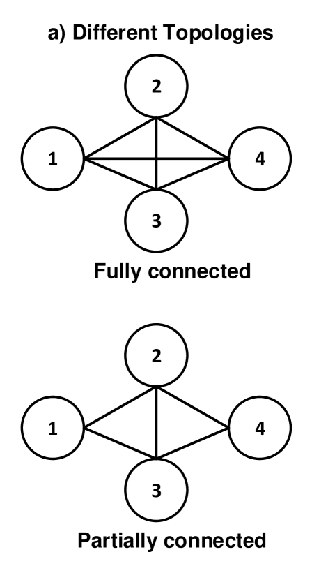
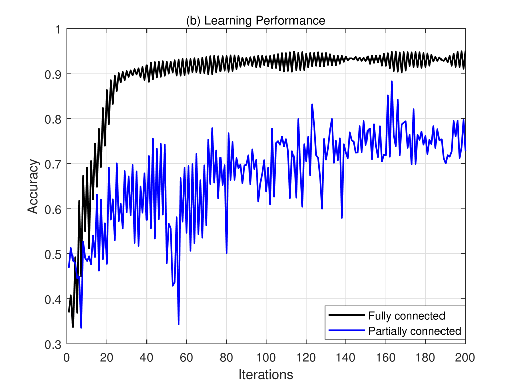
Figure 7: Typical network topologies of the UAVs for model dissemination and their FL accuracy.

We also evaluate the learning accuracy of FedMoD on different network topologies of the UAVs as shown in Fig. 7(a). We consider fully connected network where all the UAVs are connected and partially connected network where UAV $4$ is not connected to UAV $1$. In this figure, we perform $4$ different rounds of dissemination. As shown in Fig. 7(b), we see that within a given number of global iterations, a more connected network topology achieves a higher test accuracy. This is because more model information is collected from neighboring UAVs in each round of inter-UAV model aggregation. It is also observed that when $\alpha$ is greater than $4$, the test accuracy of the partially connected network can approach the case with a fully-connected network. Therefore, based on the network topology of UAVs, we can choose a suitable value of $\alpha$ to balance between the number of inter-cluster UAV aggregation and learning performance.

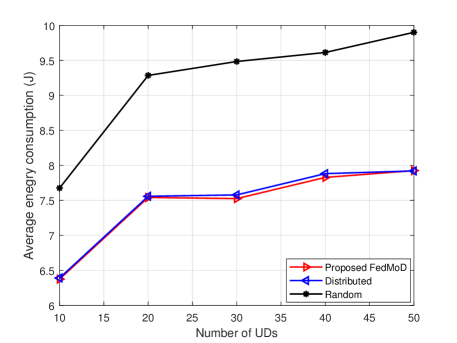
Figure 8: Average energy consumption vs. number of UDs.

In Fig. 8, we plot the energy consumption of the proposed and benchmark schemes versus the number of UDs for a network of $4$ UAVs and $4$ RRBs per UAV. From the objective function of problem P1, we can observe that an efficient radio resource management scheme leads to a lower energy consumption. Hence, from Fig. 8, we observe that for FedMoD, the average energy consumption is minimized. Such an observation is because the proposed schemes judiciously allocate LOS UDs to the UAVs and their available RRBs as well as D2D communications. In particular, the random scheme has the largest energy consumption because it randomly schedules the UDs to the UAVs and their available RRBs. Accordingly, from energy consumption perspective, it is inefficient to consider a random radio resource management scheme. From Fig. 8, it is observed that the proposed centralized scheduling FedMoD and distributed FedMoD schemes offer the same energy consumption performances for the same number of UDs. Such an observation can be explained by the following argument. When we have a large number of UDs, the probability that a UD is scheduled to more than one UAV decreases. As a result, the conflict among UAVs and the likelihood of scheduling UDs to the wrong UAV decreases. As an insight from this figure, a distributed radio resource management scheme is a suitable alternative for scheduling the LOS UDs to the UAVs, especially for large-scale networks.

VII Conclusion

In this paper, we developed a novel decentralized FL scheme, called FedMoD, which maintains convergence speed and reduces energy consumption of FL in mmWave ATINs. Specifically, we proposed a FedMoD scheme based on inter-cluster UAV communications, and theoretically proved its convergence. A rate-adaptive and D2D-assisted RRM scheme was also developed to minimize the overall energy consumption of the proposed decentralized FL scheme. The presented simulation results revealed that our proposed FedMoD achieves the same accuracy as the baseline FL scheme while substantially reducing energy consumption for convergence. In addition, simulation results reveal various insights concerning how the topology of the network impacts the number of inter-cluster UAV aggregations required for the convergence of FedMoD.

Appendix A Proof of Lemma 1

By applying the global loss function to both sides of (12) and using the L-smoothness assumption, we have:

$$\mathbb{E}[F(\mathbf{\tilde{u}}(t+1))]\leq\mathbb{E}[F(\mathbf{\tilde{u}}(t))]+\mathbb{E}\bigg{\langle}\triangledown F(\mathbf{\tilde{u}}(t)),-\lambda{\mathbf{G}}(t)\mathbf{m}\bigg{\rangle}$$

$$+\frac{L}{2}\mathbb{E}\lVert\lambda{\mathbf{G}}(t)\mathbf{m}\lVert^{2}_{2}=\mathbb{E}[F(\mathbf{\tilde{u}}(t))]-\delta\mathbb{E}\bigg{\langle}\triangledown F(\mathbf{\tilde{u}}(t)),\mathbb{E}[{\mathbf{G}}(t)\mathbf{m}]\bigg{\rangle}$$

$$+\frac{\lambda^{2}L}{2}\mathbb{E}\bigg{\lVert}\mathbf{G}(t)\mathbf{m}-\triangledown\tilde{\mathbf{F}}(t)\mathbf{m}+\triangledown\tilde{\mathbf{F}}(t)\mathbf{m}\bigg{\lVert}^{2}_{2},$$

where $\triangledown\tilde{\mathbf{F}}(t)=\bigg{[}\triangledown F_{1}(t),\triangledown F_{2}(t),\cdots,\triangledown F_{U_{inv}}(t)\bigg{]}$. Since $\mathbb{E}[\hat{\mathbf{L}}(\mathbf{\tilde{w}}_{i}(t-y))\hat{\mathbf{m}}]=\triangledown\tilde{\mathbf{L}}(\mathbf{\tilde{w}}_{i}(t-y))\hat{\mathbf{m}}$, we have the following

$$\mathbb{E}[F(\mathbf{\tilde{u}}(t+1))]=\mathbb{E}[F(\mathbf{\tilde{u}}(t))]-\lambda\mathbb{E}\bigg{\langle}\triangledown F(\mathbf{\tilde{u}}(t)),\triangledown\tilde{\mathbf{F}}(t)\mathbf{m}\bigg{\rangle}$$

$$+\frac{\lambda^{2}L}{2}\mathbb{E}\bigg{\lVert}{\mathbf{G}}(t)\mathbf{m}-\triangledown\tilde{\mathbf{F}}(t)\mathbf{m}\bigg{\lVert}^{2}_{2}+\frac{\lambda^{2}L}{2}\lVert\triangledown\tilde{\mathbf{F}}(t)\mathbf{m}\lVert^{2}_{2},$$

where $\frac{\lambda^{2}L}{2}\mathbb{E}\bigg{\lVert}{\mathbf{G}}(t)\mathbf{m}-\triangledown\tilde{\mathbf{F}}(t)\mathbf{m}+\triangledown\tilde{\mathbf{F}}(t)\mathbf{m}\bigg{\lVert}^{2}_{2}=\frac{\lambda^{2}L}{2}\mathbb{E}\bigg{\lVert}{\mathbf{G}}(t)\mathbf{m}-\triangledown\tilde{\mathbf{F}}(t)\mathbf{m}\bigg{\lVert}^{2}_{2}+\frac{\lambda^{2}L}{2}\mathbb{E}\lVert\triangledown\tilde{\mathbf{F}}(t)\mathbf{m}\lVert^{2}_{2}$. This is becasue $\mathbb{E}[\mathbf{G}(t)\mathbf{m}]=\triangledown\tilde{\mathbf{F}}(t)\mathbf{m}$, thus the cross-terms of $\mathbf{G}(t)\mathbf{m}$ and $\triangledown\tilde{\mathbf{F}}(t)\mathbf{m}$ are zero. Thus, we have

$$\mathbb{E}[F(\mathbf{\tilde{u}}(t+1))]=\mathbb{E}[F(\mathbf{\tilde{w}}(t))]-\delta\mathbb{E}\bigg{\langle}\triangledown F(\mathbf{\tilde{u}}(t)),$$

$$\sum_{u=1}^{N_{inv}}m_{u}\triangledown F_{u}(\mathbf{\tilde{u}}_{u}(t))\bigg{\rangle}+\frac{\lambda^{2}L}{2}\mathbb{E}\bigg{\lVert}\sum_{u=1}^{U_{inv}}m_{u}\bigg{(}g(\mathbf{\tilde{u}}_{u}(t))$$

$$-\triangledown F(\mathbf{\tilde{w}}_{u}(t))\bigg{)}\bigg{\lVert}^{2}_{2}+\frac{\lambda^{2}L}{2}\lVert\triangledown\tilde{\mathbf{F}}(t)\mathbf{m}\lVert^{2}_{2}$$

$$=\mathbb{E}[F(\mathbf{\tilde{u}}(t))]-\lambda\mathbb{E}\bigg{\langle}\triangledown F(\mathbf{\tilde{u}}(t)),\sum_{u=1}^{U_{inv}}m_{u}\triangledown F_{i}(\mathbf{\tilde{w}}_{u}(t))\bigg{\rangle}$$

$$+\frac{\lambda^{2}L}{2}\sum_{u=1}^{U_{inv}}m^{2}_{u}\mathbb{E}\bigg{\lVert}g(\mathbf{\tilde{w}}_{u}(t))-\triangledown F_{u}(\mathbf{\tilde{w}}_{u}(t))\bigg{\lVert}^{2}_{2}+\frac{\lambda^{2}L}{2}\lVert\triangledown\tilde{\mathbf{F}}(t)\mathbf{m}\lVert^{2}_{2}.$$

From Assumption 3, we have $\mathbb{E}\bigg{\lVert}g(\mathbf{\tilde{w}}_{u}(t))-\triangledown F_{u}(\mathbf{\tilde{w}}_{u}(t))\bigg{\lVert}^{2}_{2}\leq\sigma^{2}$. Also, $\mathbf{s}^{T}\mathbf{k}=\frac{1}{2}\lVert\mathbf{s}\lVert^{2}_{2}+\frac{1}{2}\lVert\mathbf{k}\lVert^{2}_{2}-\frac{1}{2}\lVert\mathbf{s}-\mathbf{k}\lVert^{2}_{2}$. Thus, we have $\lambda\mathbb{E}\bigg{\langle}\triangledown F(\mathbf{\tilde{u}}(t)),\sum_{u=1}^{U_{inv}}m_{u}\triangledown F_{u}(\mathbf{\tilde{w}}_{u}(t))\bigg{\rangle}=\frac{\lambda}{2}\lVert\triangledown F(\mathbf{\tilde{u}}(t))\lVert^{2}_{2}\\ +\frac{\lambda}{2}\mathbb{E}\lVert\sum_{u=1}^{U_{inv}}m_{u}\triangledown F(\mathbf{\tilde{w}}_{u}(t))\lVert^{2}_{2}-\frac{\lambda}{2}\mathbb{E}\bigg{\lVert}\triangledown F(\mathbf{\tilde{u}}(t))-\sum_{u=1}^{U_{inv}}m_{u}\triangledown F(\mathbf{\tilde{w}}_{u}(t))\bigg{\lVert}^{2}_{2}$. With such a constraint, we can have

$$\mathbb{E}[F(\mathbf{\tilde{u}}(t+1))]\leq\mathbb{E}[F(\mathbf{\tilde{u}}(t))]-\bigg{(}\frac{\lambda}{2}\lVert\triangledown F(\mathbf{\tilde{u}}(t))\lVert^{2}_{2}$$

$$+\frac{\lambda}{2}\mathbb{E}\bigg{\lVert}\sum_{u=1}^{U_{inv}}m_{u}\triangledown F(\mathbf{\tilde{u}}_{u}(t))\bigg{\lVert}^{2}_{2}-\frac{\lambda}{2}\mathbb{E}\bigg{\lVert}\triangledown F(\mathbf{\tilde{u}}(t))$$

$$-\sum_{u=1}^{U_{inv}}m_{u}\triangledown F(\mathbf{\tilde{w}}_{i}(t))\bigg{\lVert}^{2}_{2}\bigg{)}+\frac{\lambda^{2}L}{2}\sum_{u=1}^{U_{inv}}m^{2}_{u}\sigma^{2}+\frac{\lambda^{2}L}{2}\lVert\triangledown\tilde{\mathbf{F}}(t)\mathbf{m}\lVert^{2}_{2}$$

$$\leq\mathbb{E}[F(\mathbf{\tilde{u}}(t))]-\bigg{(}\frac{\lambda}{2}\lVert\triangledown F(\mathbf{\tilde{u}}(t))\lVert^{2}_{2}+\frac{\lambda}{2}\mathbb{E}\bigg{\lVert}\sum_{u=1}^{U_{inv}}m_{u}\triangledown F(\mathbf{\tilde{w}}_{u}(t))\bigg{\lVert}^{2}_{2}$$

$$-\frac{\lambda}{2}\mathbb{E}\bigg{\lVert}\sum_{u=1}^{U_{inv}}m_{u}\bigg{(}\triangledown F(\mathbf{\tilde{u}}(t))-\triangledown F(\mathbf{\tilde{w}}_{u}(t))\bigg{)}\bigg{\lVert}^{2}_{2}\bigg{)}$$

$$+\frac{\lambda^{2}L}{2}\sum_{u=1}^{U_{inv}}m^{2}_{u}\sigma^{2}+\frac{\lambda^{2}L}{2}\mathbb{E}\lVert\triangledown\sum_{u=1}^{U_{inv}}m_{u}\triangledown F_{u}(\mathbf{\tilde{w}}_{u}(t))\lVert^{2}_{2}.$$

We denote $\tilde{Q}=\mathbb{E}\lVert\triangledown\sum_{i=1}^{U_{inv}}m_{u}\triangledown F_{u}(\mathbf{\tilde{w}}_{u}(t))\lVert^{2}_{2}$, we have the following

$$\mathbb{E}[F(\mathbf{\tilde{u}}(t+1))]\leq\mathbb{E}[F(\mathbf{\tilde{u}}(t))]-\frac{\lambda}{2}\lVert\triangledown F(\mathbf{\tilde{u}}(t))\lVert^{2}_{2}-\bigg{(}\frac{\lambda}{2}-\frac{\lambda^{2}L}{2}\bigg{)}\tilde{Q}$$

$$+\frac{\lambda}{2}\mathbb{E}\bigg{\lVert}\sum_{u=1}^{U_{inv}}m_{u}\bigg{(}\triangledown F(\mathbf{\tilde{u}}(t))-\triangledown F(\mathbf{\tilde{w}}_{u}(t))\bigg{)}\bigg{\lVert}^{2}_{2}+\frac{\lambda^{2}L}{2}\sum_{u=1}^{U_{inv}}m^{2}_{u}\sigma^{2}$$

$$=\mathbb{E}[F(\mathbf{\tilde{u}}(t))]-\frac{\lambda}{2}\lVert\triangledown F(\mathbf{\tilde{u}}(t))\lVert^{2}_{2}-\bigg{(}\frac{\lambda}{2}-\frac{\lambda^{2}L}{2}\bigg{)}\tilde{Q}$$

$$+\frac{\lambda}{2}\mathbb{E}\bigg{\lVert}\sum_{u=1}^{U_{inv}}m_{u}\mathbb{E}\bigg{\lVert}\triangledown F(\mathbf{\tilde{u}}(t))-\triangledown F(\mathbf{\tilde{w}}_{i}(t))\bigg{\lVert}+\frac{\lambda^{2}L}{2}\sum_{u=1}^{U_{inv}}m^{2}_{u}\sigma^{2}$$

$$\leq\mathbb{E}[F(\mathbf{\tilde{u}}(t))]-\frac{\lambda}{2}\lVert\triangledown F(\mathbf{\tilde{u}}(t))\lVert^{2}_{2}-\bigg{(}\frac{\lambda}{2}-\frac{\lambda^{2}L}{2}\bigg{)}\tilde{Q}$$

$$+\frac{\lambda}{2}\mathbb{E}\bigg{\lVert}\sum_{u=1}^{U_{inv}}m_{u}\mathbb{E}\bigg{\lVert}\mathbf{\tilde{u}}(t)-\mathbf{\tilde{w}}_{u}(t)\bigg{\lVert}+\frac{\lambda^{2}L}{2}\sum_{u=1}^{U_{inv}}m^{2}_{u}\sigma^{2}.$$

The last inequality holds because of the L- smoothness assumption of the local loss function. We conclude the proof by moving $\mathbb{E}[F(\mathbf{\tilde{u}}(t))]$ to the left hand side (LHS), thus we will have

$$\mathbb{E}[F(\mathbf{\tilde{u}}(t+1))]-\mathbb{E}[F(\mathbf{\tilde{u}}(t))]\leq\frac{-\lambda}{2}\mathbb{E}\lVert\triangledown F(\mathbf{\tilde{u}}(t))\lVert^{2}_{2}$$

$$+\frac{\lambda^{2}L}{2}\sum_{u=1}^{{U_{inv}}}m_{u}\sigma^{2}-\frac{\lambda}{2}(1-\lambda L)\tilde{Q}+\frac{\lambda L^{2}}{2}\mathbb{E}\bigg{\lVert}\mathbf{\tilde{w}}(t)(\mathbf{I}-\mathbf{M})\bigg{\lVert}^{2}_{\mathbf{M}}.$$ (A.1)

References

- [1] L. Godage, “Global Unmanned Aerial Vehicle Market (UAV) Industry Analysis and Forecast (2018–2026),” Mont. Ledger Boston, MA, USA, 2019.
- [2] M. Z. Hassan et al., “Interference management in cellular-connected Internet-of-drones network with drone clustering and uplink rate-splitting multiple access,” IEEE Internet Things of Journal, vol. 9, no. 1, pp. 16060-16079, Sept. 2022.
- [3] S. Zhang et al., “Cellular-enabled UAV communication: A connectivity-constrained trajectory optimization perspective,” IEEE Trans. Commun., vol. 67, no. 3, pp. 2580–2604, Mar. 2019.
- [4] Technical Specification Group Services and System Aspects; Unmanned Aerial System (UAS) Support in 3GPP (Release 17), Standard 3GPP TS 22.125, 3rd Generation Partnership Project, Dec. 2019. [Online] Available: https://www.3gpp.org/ftp/Specs/archive/22 series/22.125/.
- [5] Z. Xiao et al., “Enabling UAV cellular with millimeter-wave communication: Potentials and approaches,” IEEE Commun. Mag., vol. 54, no. 5, pp. 66–73, May 2016.
- [6] B. McMahan et al., “Communication-efficient learning of deep networks from decentralized data,” 20th International Conference on Artificial Intelligence and Statistics, pp. 1273-1282, 2017.
- [7] S. Niknam et al., “Federated learning for wireless communications: Motivation, opportunities, and challenges,” IEEE Commun. Mag., vol. 58, no. 6, pp. 46–51, Jun. 2020.
- [8] Y. Qu et al., “Decentralized federated learning for UAV networks: Architecture, challenges, and opportunities,”IEEE Netw., vol. 35, no. 6, pp. 156-162, Nov. 2021.
- [9] P. Chhikara et al., “Federated learning and autonomous uavs for hazardous zone detection and AQI prediction in IoT environment,” IEEE Internet of Things J., vol. 8, no. 20, pp. 15456-15467, Oct. 2021.
- [10] W. Y. B. Lim et al., “UAV-assisted communication efficient federated learning in the era of the artificial intelligence of things,” IEEE Netw., vol. 35, no. 5, pp. 188–195, Oct. 2021.
- [11] C. B. Issaid et al., “Local stochastic ADMM for communication-efficient distributed learning,” IEEE Wireless Commun. and Netw. Conf. (WCNC), Austin, Tx, 2022.
- [12] M. M. Wadu et al., “Joint client scheduling and resource allocation under channel uncertainty in federated learning,” IEEE Trans. Commun., vol. 69, no. 9, pp. 5962–5974, Sep. 2021.
- [13] M. Chen et al., “A joint learning and communications framework for federated learning over wireless networks,” IEEE Trans. on Wireless Commun. vol. 20, no. 1, pp. 269-283, Jan. 2021.
- [14] M. Chen et al. “Convergence time optimization for federated learning over wireless networks,” IEEE Trans. Wireless Commun., vol. 20, no. 4, pp. 2457 - 2471, Apr. 2021.
- [15] S. Wang et al., “Adaptive federated learning in resource constrained edge computing systems,” IEEE J. Sel. Areas Commun., vol. 37, no. 6, pp. 1205-1221, Jun. 2019.
- [16] Z. Yang et al., “Energy efficient federated learning over wireless communication networks,” IEEE Trans. on Wireless Commun., vol. 20, no. 3, pp. 1935-1949, Mar. 2021.
- [17] J. Yao and N. Ansari, “Enhancing federated learning in fog-aided IoT by CPU frequency and wireless power control,” IEEE Int. of Things J., vol. 8, no. 5, pp. 3438-3445, Mar. 2021.
- [18] M. S. Al-Abiad et al.,“‘Energy efficient resource allocation for federated learning in NOMA enabled and relay-assisted internet of things networks”, IEEE Int. of Things J. (accepted for publication).
- [19] M. S. H. Abad et al., “Hierarchical federated learning across heterogeneous cellular networks,” [Online]. Available: https://arxiv.org/pdf/1909.02362.
- [20] L. Liu et al. “Client-edge-cloud hierarchical federated learning,” IEEE Int. Conf. Commun., Dublin, 2020.
- [21] S. Hosseinalipour et al., “From federated to fog learning: Distributed machine learning over heterogeneous wireless networks,” IEEE Commun. Mag., vol. 58, no. 12, pp. 41-47, Dec. 2020.
- [22] S. Luo et al. “HFEL: Joint edge association and resource allocation for cost-efficient hierarchical federated edge learning,” IEEE Trans. Wireless Commun., vol. 19, no. 10, pp. 6535-6548, Oct. 2020.
- [23] S. Liu et al., “Joint user association and resource allocation for wireless hierarchical federated learning with IID and non-IID data,” IEEE Trans. Wireless Commun. (accepted for publication).
- [24] F. P. -C. Lin et al., “Semi-decentralized federated learning with cooperative D2D local model aggregations,” IEEE J. Sel. Areas Commun., vol. 39, no. 12, pp. 3851-3869, Dec. 2021.
- [25] Y. Sun et al., “Semi-decentralized federated edge learning for fast convergence on non-IID data,” [Online]. Available: https://arxiv.org/pdf/2104.12678.pdf.
- [26] Y. Sun et al., “Semi-decentralized federated edge learning with data and device heterogeneity,” [Online]. Available: https://arxiv.org/pdf/2112.10313.pdf.
- [27] M. S. Al-Abiad et al., “Coordinated scheduling and decentralized federated learning using conflict clustering graphs in fog-assisted IoD networks,” IEEE Trans. Veh. Technol. (accepted for publications).
- [28] M. S. Al-Abiad, M. J. Hossain, and S. Sorour, “Cross-layer cloud offloading with quality of service guarantees in Fog-RANs,” in IEEE Trans. on Commun., vol. 67, no. 12, pp. 8435-8449, Dec. 2019.
- [29] A. Douik etl, ”Distributed hybrid scheduling in multi-cloud networks using conflict graphs,” in IEEE Trans. on Commun., vol. 66, no. 1, pp. 209-224, Jan. 2018.
- [30] J. Sabzehali etl, “3D placement and orientation of mmWave-Based UAVs for guaranteed loS coverage,” in IEEE Wireless Commun. Letters, vol. 10, no. 8, pp. 1662-1666, Aug. 2021.
- [31] N. Cherif etl, “Downlink coverage and rate analysis of an aerial user in vertical heterogeneous networks (VHetNets),” in IEEE Trans. on Wireless Commu., vol. 20, no. 3, pp. 1501-1516, Mar. 2021.
- [32] M. Mozaffari etl, “Efficient deployment of multiple unmanned aerial vehicles for optimal wireless coverage,” IEEE Commun. Lett., vol. 20, no. 8, pp. 1647–1650, Aug. 2016.
- [33] V. V. Chetlur etl, “Coverage and rate analysis of downlink cellular Vehicle-to-Everything (C-V2X) communication,” in IEEE Trans. Wireless Commun., vol. 19, no. 3, pp. 1738–1753, Mar. 2020.
- [34] M. S. Al-Abiad, M. Z. Hassan, and M. J. Hossain, ”Task offloading optimization in NOMA-enabled dual-hop mobile edge computing system using conflict graph,” in IEEE Trans. on Wireless Commun., 2022, doi: 10.1109/TWC.2022.
- [35] M. S. Al-Abiad et al., “Cross-layer network codes for completion time minimization in device-to-device networks,” in IEEE Access, vol. 10, pp. 61567-61584, 2022.
- [36] M. S. Al-Abiad et al., “Decentralized aggregation for energy-efficient federated learning via overlapped clustering and D2D communications,” TechRxiv. Preprint. https://doi.org/10.36227/techrxiv.19740394.v1, May 2022.
- [37] M. S. Al-Abiad etl, “Energy efficient resource allocation for federated learning in NOMA enabled and relay-assisted internet of things networks”, in IEEE Int. of Things Journal, 2022.
- [38] A. P. Chandrakasan, S. Sheng, and R.W. Brodersen, “Low-power CMOS digital design,” IEEE J. Solid-State Circuits, vol. 27, no. 4, pp. 473-484, Apr. 1992.
- [39] T. D. Burd and R. W. Brodersen, “Processor design for portable systems,” J. VLSI Signal Process Syst. Signal Image Video Technol., vol. 13, no. 2, pp. 203-221, Aug. 1996.
- [40] M. Z. Hassan, G. Kaddoum and O. Akhrif, “Interference management in cellular-connected internet-of-drones networks with drone-pairing and uplink rate-splitting multiple access,” in IEEE Internet Things J., Apr. 2022.
- [41] M. B. Ghorbel et al., ”Joint position and travel path optimization for energy efficient wireless data gathering using unmanned aerial vehicles,” in IEEE Trans. Veh. Technol., vol. 68, no. 3, pp. 2165-2175, Mar. 2019.
- [42] H. Ghazzai et al., “Energy-efficient management of unmanned aerial vehicles for underlay cognitive radio systems,” IEEE Trans. Green Commun. Netw., vol. 1, no. 4, pp. 434-443, Dec. 2017.