Abstract

The sensor placement problem is a common problem that arises when monitoring correlated phenomena, such as temperature, precipitation, and salinity. Existing approaches to this problem typically formulate it as the maximization of information metrics, such as mutual information (MI), and use optimization methods such as greedy algorithms in discrete domains, and derivative-free optimization methods such as genetic algorithms in continuous domains. However, computing MI for sensor placement requires discretizing the environment, and its computation cost depends on the size of the discretized environment. This limitation restricts these approaches from scaling to large problems. We have uncovered a novel connection between the sensor placement problem and sparse Gaussian processes (SGP). Our approach leverages SGPs and is gradient-based, which allows us to efficiently find solution placements in continuous environments. We generalize our method to also handle discrete environments. Our experimental results on four real-world datasets demonstrate that our approach generates sensor placements consistently on par with or better than the prior state-of-the-art approaches in terms of both MI and reconstruction quality, all while being significantly faster. Our computationally efficient approach enables both large-scale sensor placement and fast robotic sensor placement for informative path planning algorithms.

1 Introduction

Meteorology and climate change are concerned with monitoring correlated environmental phenomena such as temperature, ozone concentration, soil chemistry, ocean salinity, and fugitive gas density [Krause et al., 2008, Ma et al., 2017, Suryan and Tokekar, 2020, Whitman et al., 2021, Jakkala and Akella, 2022]. However, it is often too expensive and, in some cases, even infeasible to monitor the entire environment with a dense sensor network. We therefore aim to determine strategic locations for a sparse set of sensors so that the data from these sensors gives us the most accurate estimate of the phenomenon over the entire environment. We address this sensor placement problem for correlated environment monitoring.

The sensor placement problem in correlated environments is a fundamental problem with diverse and important applications. For example, informative path planning (IPP) is a crucial problem in robotics that involves identifying informative sensing locations for robots while considering travel distance constraints [Ma et al., 2017]. Similar sensor placement problems arise in autonomous robot inspection and monitoring of 3D surfaces [Zhu et al., 2021], for example, when a robot must monitor stress fractures on an aircraft body. Recently a sensor placement approach has even been used to learn dynamical systems in a sample-efficient manner [Buisson-Fenet et al., 2020].

An effective approach to address the sensor placement problem in correlated environments is to use Gaussian processes (GPs) [Husain and Caselton, 1980, Shewry and Wynn, 1987, Wu and Zidek, 1992, Krause et al., 2008]. We can capture the correlations of the environment using the GP’s kernel function and then leverage the GP to estimate information metrics such as mutual information (MI). Such metrics can be used to quantify the amount of new information that can be obtained from each candidate sensor location. However, computing MI using GPs is very expensive as it requires the inversion of large covariance matrices whose size increases with the environment’s discretization resolution. Having faster sensor placement approaches would enable addressing the abovementioned applications, which require a large number of sensor placements or a fine sensor placement precision that is infeasible with discrete approaches.

Sparse Gaussian processes (SGPs) [Quinonero-Candela et al., 2007, Bui et al., 2017] are a computationally efficient variant of GPs. Therefore, one might consider using SGPs instead of GPs in GP-based sensor placement approaches. However, a naive replacement of GPs with SGPs is not always possible or efficient. This is because SGPs must be retrained for each evaluation of MI. In sensor placement approaches, MI is often evaluated repeatedly, making SGPs computationally more expensive than GPs for sensor placement. As a result, even though SGPs have been studied for over two decades, SGPs have not yet been widely adopted for sensor placement despite their potential advantages.

The objective of this paper is to develop an efficient approach for sensor placement in correlated environments. We present an efficient gradient-based approach for sensor placement in continuous environments by uncovering the connection between SGPs and sensor placement problems. We generalize our method to also efficiently handle sensor placement in discrete environments.

2 Problem Statement

Consider a correlated stochastic process $\Psi$ over an environment $\mathcal{V}\subseteq\mathbb{R}^{d}$ modeling a phenomenon such as temperature. The sensor placement problem is to select a set $\mathcal{A}$ of $s$ sensor locations $\{\mathbf{x}_{i}\in\mathcal{V},i=1,...,s\}$ so that the data $y_{i}\in\mathbb{R}$ collected at these locations gives us the most accurate estimate of the phenomenon at every location in the environment. We consider estimates with the lowest root-mean-square error (RMSE) to be the most accurate. An ideal solution to this sensor placement problem should have the following key properties:

1. The approach should be computationally efficient and produce solutions with low RMSE. Since the environment is correlated, this should also result in the solution sensor placements being well separated to ensure that the sensors collect only novel data that is crucial for accurately reconstructing the data field.

2. The approach should handle both densely and sparsely labeled environments. In a densely labeled environment, we have labeled data at every location in the environment. In a sparsely labeled environment, we have labeled data that is sufficient only to capture the correlations in the environment, or we have domain knowledge about how the environment is correlated.

3. The approach should handle both continuous sensor placements $\mathcal{A}\subseteq\mathcal{V}$, where the sensors can be placed anywhere in the environment, and discrete sensor placements $\mathcal{A}\subseteq\mathcal{S}\subseteq\mathcal{V}$, where the sensors can only be placed at a subset of a pre-defined set of locations $\mathcal{S}$.

3 Related Work

Early approaches to the sensor placement problem [Bai et al., 2006, Ramsden, 2009] used geometric models of the sensor’s field of view to account for the region covered by each sensor and used computational geometry or integer programming methods to find solutions. Such approaches proved useful for problems such as the art gallery problem [de Berg et al., 2008], which requires one to place cameras so that the entire environment is visible. However, these approaches do not consider the spatial correlations in the environment.

This problem is also studied in robotics [Cortes et al., 2004, Breitenmoser et al., 2010, Sadeghi et al., 2022]. Similar to geometric approaches, authors focus on coverage by leveraging Voronoi decompositions [de Berg et al., 2008]. A few authors [Schwager et al., 2017, Salam and Hsieh, 2019], have even considered Gaussian kernel functions, but they did not leverage the full potential of Gaussian processes.

Gaussian process (GP) based approaches addressed the limitations of geometric model-based sensor placement approaches by learning the spatial correlations in the environment. The learned GP is then used to quantify the information gained from each sensor placement while accounting for the correlations of the data field. However, these methods require one to discretize the environment and introduce severe computational scaling issues. Our method finds sensor locations in continuous spaces and overcomes the computational scaling issues.

Early GP-based approaches [Shewry and Wynn, 1987, Wu and Zidek, 1992] placed sensors at the highest entropy locations. However, since GPs have high variance in regions of the environment far from the locations of the training samples, such approaches tended to place sensors at the sensing area’s borders, resulting in poor coverage of the area of interest. [Krause et al., 2008] used mutual information (MI) computed with GPs to select sensor locations with the maximal information about all the unsensed locations in the environment. The approach avoided placing the sensors at the environment’s boundaries and outperformed all earlier approaches in terms of reconstruction quality and computational cost.

[Whitman et al., 2021] recently proposed an approach to model spatiotemporal data fields using a combination of sparse Gaussian processes and state space models. They then used the spatiotemporal model to sequentially place sensors in a discretized version of the environment. Although their spatiotemporal model of the environment resulted in superior sensor placements, the combinatorial search becomes prohibitively large and limits the size of the problems that can be solved using their method.

Sensor placement in continuous environments has been addressed in the context of informative path planning using gradient-free optimization methods such as evolutionary algorithms [Hitz et al., 2017] and Bayesian optimization [Francis et al., 2019]. However, both approaches maximized MI computed using GPs, which is computationally expensive. In addition, evolutionary algorithms and Bayesian optimization are known to have poor scalability.

4 Background: GPs and SGPs

Gaussian processes (GPs) [Rasmussen and Williams, 2005] are a non-parametric Bayesian approach that we can use for regression, classification, and generative problems. Suppose we are given a regression task’s training set $\mathcal{D}=\{(\mathbf{x}_{i},y_{i}),i=1,...,n\}$ with $n$ data samples consisting of inputs $\mathbf{x}_{i}\in\mathbb{R}^{d}$ and noisy labels $y_{i}\in\mathbb{R}$, such that, $y_{i}=f(\mathbf{x}_{i})+\epsilon_{i}$, where $\epsilon_{i}\sim\mathcal{N}(0,\sigma^{2}_{\text{noise}})$. Here $\sigma^{2}_{\text{noise}}$ is the variance of the independent additive Gaussian noise in the observed labels $y_{i}$, and the latent function $f(\mathbf{x})$ models the noise-free function of interest that characterizes the regression dataset.

GPs model such datasets by assuming a GP prior over the space of functions that we could use to model the dataset, i.e., they assume the prior distribution over the function of interest $p(\mathbf{f}|\mathbf{X})=\mathcal{N}(0,\mathbf{K})$, where $\mathbf{f}=[f_{1},f_{2},...,f_{n}]^{\top}$ is a vector of latent function values, $f_{i}=f(\mathbf{x}_{i})$. $\mathbf{X}=[\mathbf{x}_{1},\mathbf{x}_{2},...,\mathbf{x}_{n}]^{\top}$ is a vector (or matrix) of inputs, and $\mathbf{K}\in\mathbb{R}^{n\times n}$ is a covariance matrix, whose entries $\mathbf{K}_{ij}$ are given by the kernel function $k(\mathbf{x}_{i},\mathbf{x}_{j})$.

The kernel function parameters are tuned using Type II maximum likelihood [Bishop, 2006] so that the GP accurately predicts the training dataset labels. This approach requires an inversion of a matrix of size $n\times n$, which is a $\mathcal{O}(n^{3})$ operation, where $n$ is the number of training set samples. Thus this method can handle at most a few thousand training samples.

Sparse Gaussian processes (SGPs) [Snelson and Ghahramani, 2006, Titsias, 2009, Hoang et al., 2015, Bui et al., 2017] address the computational cost issues of Gaussian processes. SGPs do this by approximating the full GP using another Gaussian process supported with $m$ data points called inducing points, where $m\ll n$. Since the SGP support set (i.e., the data samples used to estimate the training set labels) is smaller than the full GP’s support set (the whole training dataset), SGPs reduce the matrix inversion cost to $\mathcal{O}(m^{3})$.

There are multiple SGP approaches; one particularly interesting approach is the sparse variational GP (SVGP) [Titsias, 2009], a well-known approach in the Bayesian community that has had a significant impact on the sparse Gaussian process literature given its theoretical properties [Bauer et al., 2016, Burt et al., 2019].

To approximate the full GP, the SVGP approach uses a variational distribution $q$ parametrized with $m$ inducing points. The approach treats the inducing points as variational parameters instead of model parameters, i.e., the inducing points parametrize a distribution over the latent space of the SGP instead of directly parameterizing the latent space. Thus the inducing points are protected from overfitting. The SVGP approach’s mean predictions and covariances for new data samples are computed using the following equations:

$$m_{\mathbf{y}}^{q}(\mathbf{x}) =\mathbf{K}_{xm}\mathbf{K}_{mm}^{-1}\boldsymbol{\mu}\,,$$ (1)

$$k_{\mathbf{y}}^{q}(\mathbf{x},\mathbf{x}^{\prime}) =k(\mathbf{x},\mathbf{x}^{\prime})-\mathbf{K}_{xm}\mathbf{K}_{mm}^{-1}\mathbf{K}_{mx^{\prime}}+$$

$$\ \ \ \ \ \mathbf{K}_{xm}\mathbf{K}_{mm}^{-1}\mathbf{A}\mathbf{K}_{mm}^{-1}\mathbf{K}_{mx^{\prime}}\,,$$

where the covariance term subscripts indicate the input variables used to compute the covariance; $m$ corresponds to the inducing points $\mathbf{X}_{m}$ and $x$ corresponds to any other data point $\mathbf{x}$. $\boldsymbol{\mu}$ and $\mathbf{A}$ are the mean and covariance of the optimal variational distribution $q^{*}$. The approach maximizes the following evidence lower bound (ELBO) $\mathcal{F}$ to optimize the parameters of the variational distribution:

$$\mathcal{F} =\underbrace{\frac{n}{2}\log(2\pi)}_{\text{constant}}+\underbrace{\frac{1}{2}\mathbf{y}^{\top}(\mathbf{Q}_{nn}+\sigma_{\text{noise}}^{2}I)^{-1}\mathbf{y}}_{\text{data fit}}+$$ (2)

$$\underbrace{\frac{1}{2}\log|\mathbf{Q}_{nn}+\sigma_{\text{noise}}^{2}I|}_{\text{complexity term}}-\underbrace{\frac{1}{2\sigma_{\text{noise}}^{2}}Tr(\mathbf{K}_{nn}-\mathbf{Q}_{nn})}_{\text{trace term}}\,,$$

where $\mathbf{Q}_{nn}=\mathbf{K}_{nm}\mathbf{K}_{mm}^{-1}\mathbf{K}_{mn}$ and $\mathbf{K}_{mm}$ is the covariance matrix of the inducing points $\mathbf{X}_{m}$. Please refer to Bauer et al. [Bauer et al., 2016] for an in-depth analysis of the SVGP’s lower bound.

5 Method

We first present our reduction of the sensor placement problem in correlated environments to a regression problem that can be solved using SGPs. Then, we discuss how our approach satisfies each of the key properties of an ideal sensor placement solution, outlined in Section 2.

Proposition 1.

The sensor placement problem in correlated environments is equivalent to an SGP-based regression problem.

Proof.

Consider a labeled regression problem. It can be viewed as taking a finite set of data samples from a data domain and learning to map the input samples $\mathbf{x}_{i}\in\mathbb{R}^{d}$ to their corresponding labels $y_{i}\in\mathbb{R}$. An ideal regression approach would be able to use this finite training set $\mathcal{D}=\{(\mathbf{x}_{i},y_{i}),i=1,...,n\}$ to learn to map any point in the data domain to its corresponding label even if the point is not in the training set.

In our correlated sensor placement problem, we can consider the domain of our environment $\mathbb{R}^{d}$ as the data domain, and the regions that can be included in the training set as the regions within the environment $\mathcal{V}\subset\mathbb{R}^{d}$. An ideal regression model fit to such a dataset with the labels corresponding to the values of the sensed phenomenon would give us a model that can accurately predict the phenomenon within the environment $\mathcal{V}$. In the Bayesian realm, one would consider a non-parametric approach such as GPs that maximize $\log p(\mathbf{y})$ and evaluate the posterior noise-free labels $\mathbf{z}$ for any given test samples $\mathbf{X}^{*}$ as follows: $p(\mathbf{z}|\mathbf{y})=\int p(\mathbf{z}|\mathbf{f})p(\mathbf{f}|\mathbf{y})d\mathbf{f}$. Here, $\mathbf{f}$ are the latents corresponding to the training set inputs $\mathbf{X}$.

Since GPs are not computationally efficient ($\mathcal{O}(n^{3})$), we instead consider SGPs. Given a training dataset with $n$ samples, SGPs also maximize $\log p(\mathbf{y})$. However, they have the additional constraint of distilling the training dataset to only $m$ inducing points, where $m\ll n$. We can then use only the inducing points to predict the labels of the test dataset in an efficient manner (in $\mathcal{O}(nm^{2})$). In the case of sparse variational GPs (SVGPs) [Titsias, 2009], this constraint is realized as a variational distribution parametrized with $m$ inducing points. The posterior is evaluated as follows: $q(\mathbf{z})=\int p(\mathbf{z}|\mathbf{f}_{m})\phi(\mathbf{f}_{m})d\mathbf{f}_{m}$, where $\phi$ is the variational distribution learnt from the training set and $\mathbf{f}_{m}$ are the latents corresponding to the inducing points $\mathbf{X}_{m}$. As such, the inducing points are optimized by construction to approximate the training dataset accurately (Equation 2).

Suppose the inducing points are parameterized to be in the same domain as the training data. In that case, the inducing points will correspond to critical locations in the data domain, which are required to predict the training dataset accurately. This is equivalent to our sensor placement problem with $m$ sensors. Therefore, we have reduced our sensor placement problem in correlated environments to a regression problem that can be solved using SGPs. Please refer to the Supplementary for details of its theoretical ramifications.

∎

5.1 Continuous-SGP: Continuous Solutions

We leverage Proposition 1 to find the solution sensor placements in continuous environments. To ensure that our approach is computationally feasible, instead of considering every data sample in the sensor placement environment $\mathbf{x}_{i}\in\mathcal{V}$, we use a finite number of samples from a random uniform distribution $\Phi$ defined over the bounds of the environment to train the SGP. When considering the densely labeled variant of the sensor placement problem, we use the ground truth labels $\mathbf{y}$ associated with the sampled inputs $\mathbf{X}\sim\Phi(\mathcal{V})$ to train the SGP. We parametrize the inducing points to be in the same domain as the training set inputs and impose a cardinality constraint over the solution sensor placements by specifying the number of inducing points. Once the SGP is trained using gradient descent, we return the optimized inducing points as the solution placements.

This solution is inherently computationally efficient as it requires us to only train an SGP. In addition, consider the SVGP approach [Titsias, 2009], the data fit term in its lower bound $\mathcal{F}$ (Equation 2) ensures that our solution placements have low RMSE on the samples within the environment $\mathcal{V}$. The complexity term ensures that the placements are well separated to be able to collect novel data. The trace term ensures that the uncertainty about the entire environment is minimized. Also, the method leverages the environment’s covariance structure captured by the kernel function to better use the available sensors. Therefore, the method satisfies the first property of an ideal sensor placement approach detailed in Section 2.

Furthermore, note that our approach is not limited to the SVGP approach. Indeed, our solution enables leveraging the vast SGP literature to address multiple variants of the sensor placement problem. For example, we can use stochastic gradient optimizable SGPs [Hensman et al., 2013, Wilkinson et al., 2021] with our approach to address significantly large sensor placement problems, i.e., environments that require a large number of sensor placements. Similarly, we can use spatiotemporal-SVGPs [Hamelijnck et al., 2021] with our approach to efficiently optimize sensor placements for spatiotemporally correlated environments. Also, Proposition 1 enables us to bound the KL divergence between our solution for any given number of sensing locations and an ideal sensing model that senses every location in the environment:

Theorem 1.

[Burt et al., 2019] Suppose $N$ training inputs are drawn i.i.d according to input density $p(\mathbf{x})$, and $k(\mathbf{x,x})<v$ for all $\mathbf{x}\in\mathbf{X}$. Sample $M$ inducing points from the training data with the probability assigned to any set of size $M$ equal to the probability assigned to the corresponding subset by an $\epsilon$ k-Determinantal Point Process with $k=M$. With probability at least $1-\delta$,

$$KL(Q||\hat{P})\leq\frac{C(M+1)+2Nv\epsilon}{2\sigma^{2}_{n}\delta}\left(1+\frac{||\mathbf{y}||^{2}_{2}}{\sigma^{2}_{n}}\right)$$

where $C=N\sum^{\infty}_{m=M+1}\lambda_{m}$, $\lambda_{m}$ are the eigenvalues of the integral operator $\mathcal{K}$ for kernel $k$ and $p(\mathbf{x})$.

In our sensor placement problem, $Q$ is equivalent to an SVGP that can be used to predict the state of the whole environment from sensor data collected at the inducing points, and $\hat{P}$ is a GP that senses every location in the environment.

Now consider the sparsely labeled variant of our sensor placement problem. It is often the case that it is not possible to get labeled data from the whole environment. In the SVGP’s lower bound $\mathcal{F}$ (Equation 2), only the data fit term is dependent on the training set labels. The complexity and trace terms use only the input features and the kernel function. We can leverage this property of SVGPs to train them in an unsupervised manner.

In the absence of information about how the phenomenon is realized at any given location, our best source of information is the kernel function, which can tell us how the environment is correlated. We can use this information to determine regions of the environment that vary at a high frequency and those that vary at a lower frequency, thereby allowing us to determine which regions require more sensors and which regions can be monitored with only a few sensors.

GP-based sensor placement approaches require a small dataset that can be used to learn the kernel function parameters or assume that we have the domain knowledge to initialize the kernel function such that we can capture the correlations in the environment [Wu and Zidek, 1992, Krause et al., 2008]. Therefore, since we already know the kernel function parameters, even if the data fit term of the SVGP’s lower bound $\mathcal{F}$ (Equation 2) is disabled, we can still optimize the SGP’s inducing points to get informative sensor placements. As such, we set the training set labels to zero and use a zero mean function in the SGP, which will disable the data fit term. Once we do that, we only need to optimize the inducing point locations of the SGP via the complexity and trace terms of the lower bound $\mathcal{F}$. Algorithm 1 shows the pseudocode of the approach.

Input: $k_{\theta},\mathcal{V},\Phi$, $s$, $n$, $\gamma$

Output: Sensor placements $\mathcal{A}\subset\mathcal{V}$, $|\mathcal{A}|=s$

1

2$\mathbf{X}\sim\Phi(\mathcal{V})$  / / Draw $n$ unlabeled locations

3$\mathbf{X}_{m}=\text{RandomUniformSubset}(\mathbf{X},s)$

/ / Initialize the SVGP with 0 mean and 0 labeled data

4$\varphi=\mathcal{SGP}(\text{mean}=0,k_{\theta};\mathbf{X},\mathbf{y}=\mathbf{0},\mathbf{X}_{m})$

5$\textbf{Loop until}\textit{ convergence}:$

6$\quad\quad\quad\mathbf{X}_{m}\leftarrow\mathbf{X}_{m}+\gamma\nabla\mathcal{F}_{\varphi}(\mathbf{X}_{m})$

return $\mathbf{X}_{m}$

Algorithm 1 Continuous-SGP. $k_{\theta}$ is the kernel with learned parameters, $\Phi$ is a random distribution defined over the bounds of the environment $\mathcal{V}$, and $\gamma$ is the SGP learning rate.

5.2 Greedy-SGP: Greedy Discrete Solutions

Now consider the case when we want to limit the solution of the sensor placement problem to a discrete set of candidate locations, either a subset of the training points or any other arbitrary set of points. In this case, we can use the inducing points selection approach outlined in [Titsias, 2009] to handle non-differentiable data domains. The approach entails sequentially selecting the inducing points $\mathbf{X}_{m}$ from the candidate set $\mathcal{S}$ using a greedy approach (Equation 3). It considers the increment in the SVGP’s optimization bound $\mathcal{F}$ as the maximization criteria. In each iteration, we select the point $\mathbf{x}$ that results in the largest increment in the SVGP’s bound $\mathcal{F}$ upon being added to the current inducing points set $\mathbf{X}_{m}$:

$$\mathbf{X}_{m}\leftarrow\mathbf{X}_{m}\cup\{\operatorname*{arg\,max}_{\mathbf{x}\in\mathcal{S}\backslash\mathbf{X}_{m}}\mathcal{F}(\mathbf{X}_{m}\cup\{\mathbf{x}\})-\mathcal{F}(\mathbf{X}_{m})\}\,.\\$$ (3)

Here $\mathbf{X}_{m}$ is the set of inducing points/sensing locations, and $\mathcal{S}\backslash\mathbf{X}_{m}$ is the set of remaining candidate locations after excluding the current inducing points set $\mathbf{X}_{m}$.

5.3 Discrete-SGP: Gradient-based Discrete Solutions

The problem with any greedy selection algorithm is its inherently sequential selection procedure. A better solution may be possible if the initially selected inducing points are re-selected at the end of the greedy approach, or if the inducing points are all selected together while accounting for their combined effect instead of only incrementally considering the effect of the ones that were selected in the sequential approach.

Our approach to this problem is to simultaneously optimize all the inducing points in the continuous input space using gradient descent (as in Section 5.1) and map the solution to the discrete candidate solution space $\mathcal{S}$. We can map the continuous space solutions to discrete sets by treating the mapping problem as an assignment problem [Burkard et al., 2012], i.e., as a weighted bipartite matching problem. The assignment problem requires one to find the minimal cost matching of a set of items to another set of items given their pairwise costs. We compute the pairwise Euclidean distances between the continuous space inducing points and the discrete space candidate set locations $\mathcal{S}$. The distances are then used as the costs in an assignment problem. One could even use covariances that are appropriately transformed, instead of distances, in the mapping operation to account for the correlations in the environment.

The solution of the assignment problem gives us points in the discrete candidate set closest to the continuous space solution set1. Such a solution could be superior to the greedy solution since the points in the continuous space solution set are simultaneously optimized using gradient descent instead of being sequentially selected. Although the gradient-based solution could get stuck in a local optimum, in our experiments, we found that the gradient-based discrete solutions are on par or better than the greedy solutions while being substantially faster to optimize.

6 Comparison with Mutual Information

Our Greedy-SGP approach has a few interesting similarities to the mutual information (MI) based sensor placement approach [Krause et al., 2008]. The MI approach uses a full GP to evaluate MI between the sensing locations and the rest of the environment to be monitored. The MI based criteria shown below was used to greedily select sensing locations:

$$MI(\mathbf{X}_{m}\cup\{\mathbf{x}\})-MI(\mathbf{X}_{m})=H(\mathbf{x}|\mathbf{X}_{m})-H(\mathbf{x}|\mathcal{S}\backslash\mathbf{X}_{m})\,,\vspace{-2mm}$$

where $\mathbf{X}_{m}$ is the set of selected sensing locations, and $\mathcal{S}\backslash\mathbf{X}_{m}$ is the set of all candidate locations in the environment excluding the current sensor locations $\mathbf{X}_{m}$. [Krause et al., 2008] used a Gaussian process (GP) with known kernel parameters to evaluate the entropy terms. The SVGP’s optimization bound based selection criterion to obtain discrete solutions using the greedy algorithm is equivalent to maximizing the following:

$$\Delta\mathcal{F}=\text{KL}(\phi(f_{i}|\mathbf{f}_{m})||p{(f_{i}|\mathbf{y})})-\text{KL}(p(f_{i}|\mathbf{f}_{m})||p{(f_{i}|\mathbf{y})})\,.\vspace{-2mm}$$

The first KL term measures the divergence between the variational distribution $\phi$ over $f_{i}$ (the latent variable corresponding to $\mathbf{x}$) given the latents of the inducing points set $\mathbf{X}_{m}$, and the exact conditional given the training set labels $\mathbf{y}$ (the conditional uses the training set inputs $\mathbf{X}$ as well). The second term acts as a normalization term that measures the divergence between the exact conditional over $f_{i}$ given the latents of the inducing points and the same given the training labels.

A key difference between our approach and the MI approach is that we use the efficient cross-entropy (in the KL terms) to account for the whole environment. In contrast, the MI approach uses the computationally expensive entropy term $H(\mathbf{x}|\mathcal{S}\backslash\mathbf{X}_{m})$. However, the overall formulation of both approaches is similar. We validate this empirically in the experiments section.

7 Experiments

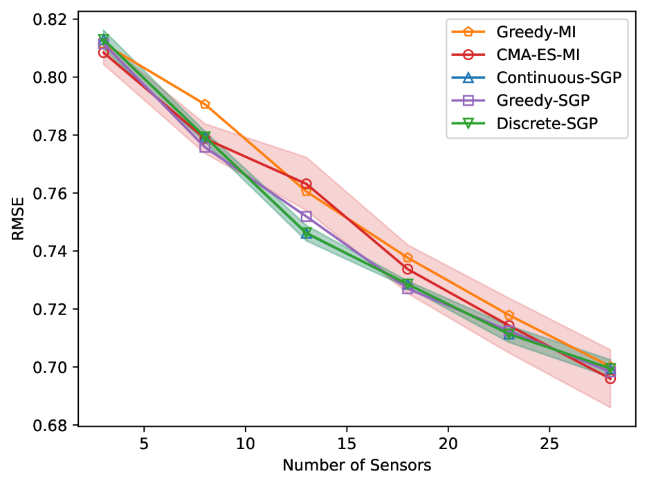
(a) Temperature dataset

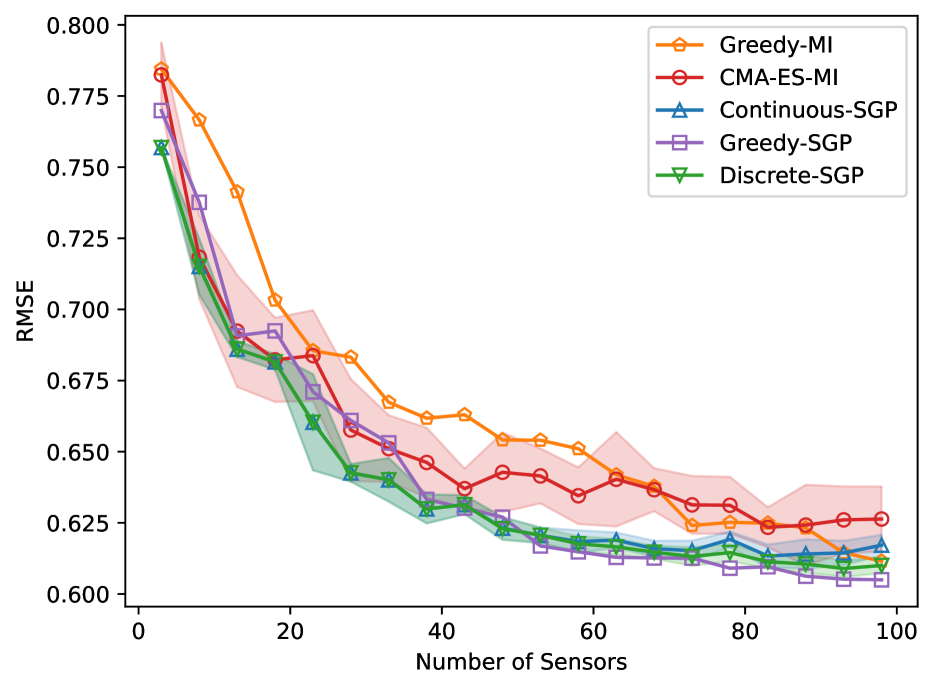
(b) Precipitation dataset

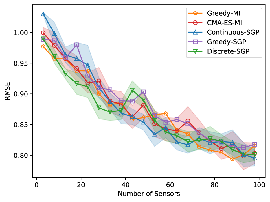
(c) Soil dataset

(d) Salinity dataset

Figure 1: The mean and standard deviation of the RMSE vs number of sensors for the Intel, precipitation, soil, and salinity datasets (lower is better).

(a) Temperature dataset

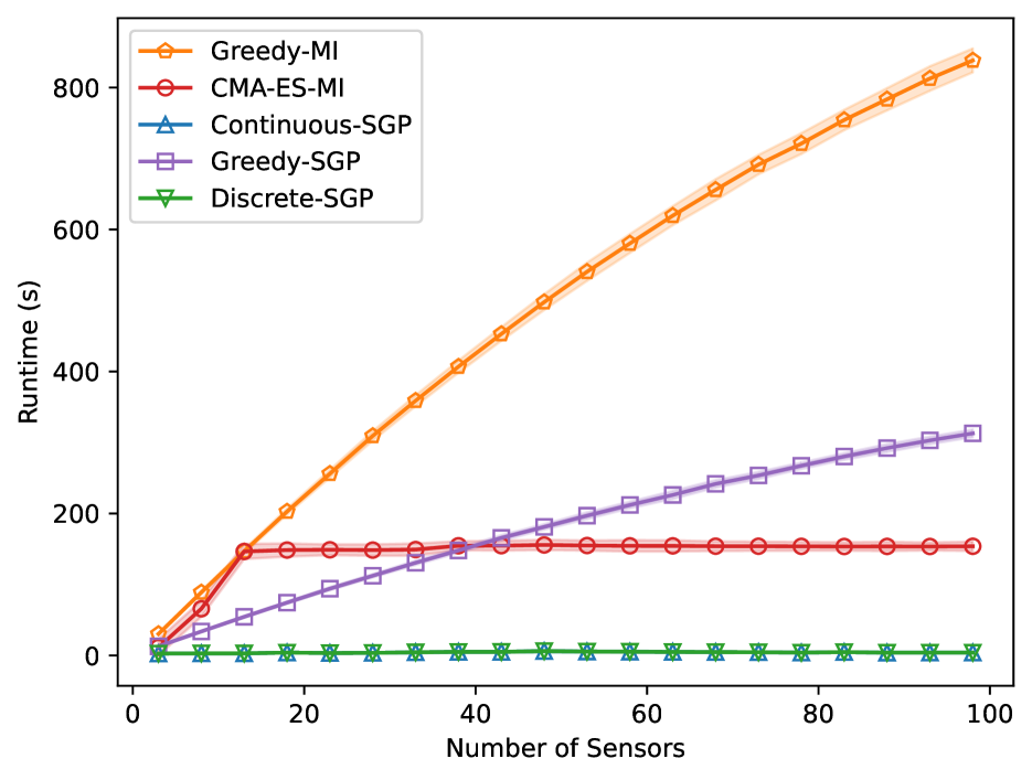
(b) Precipitation dataset

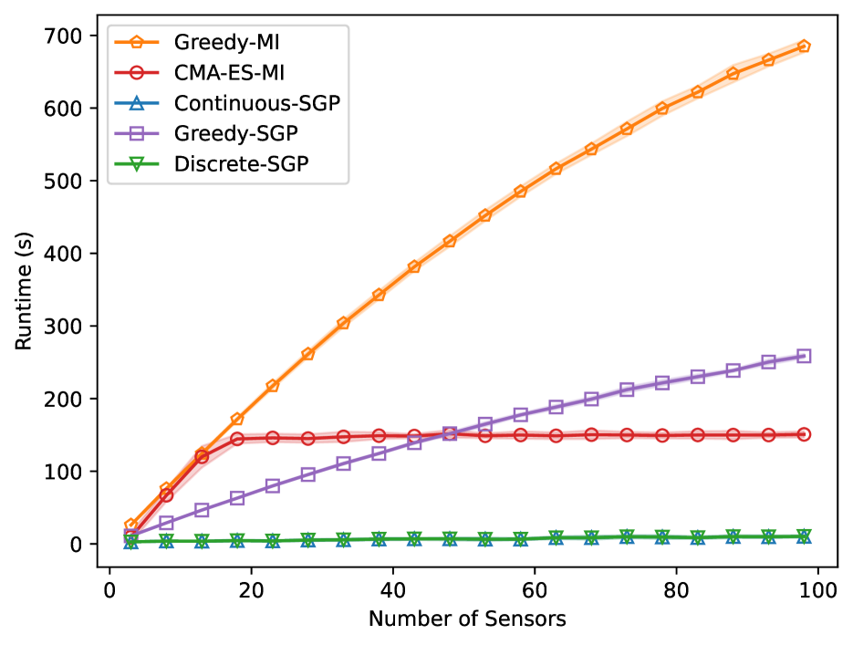
(c) Soil dataset

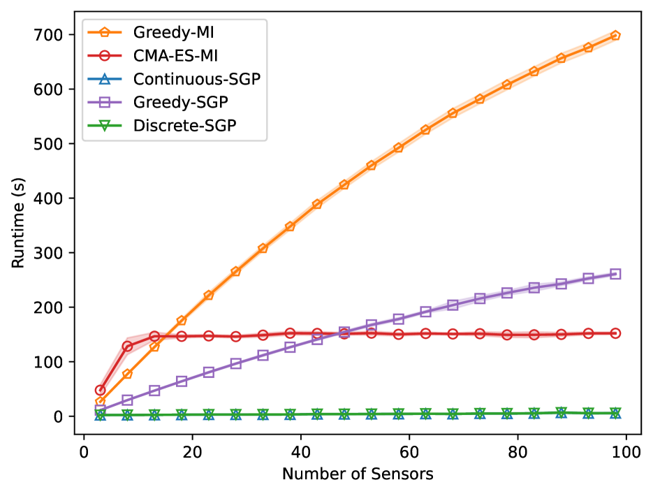
(d) Salinity dataset

Figure 2: The mean and standard deviation of the Runtime vs number of sensors for the Intel, precipitation, soil, and salinity datasets (lower is better).

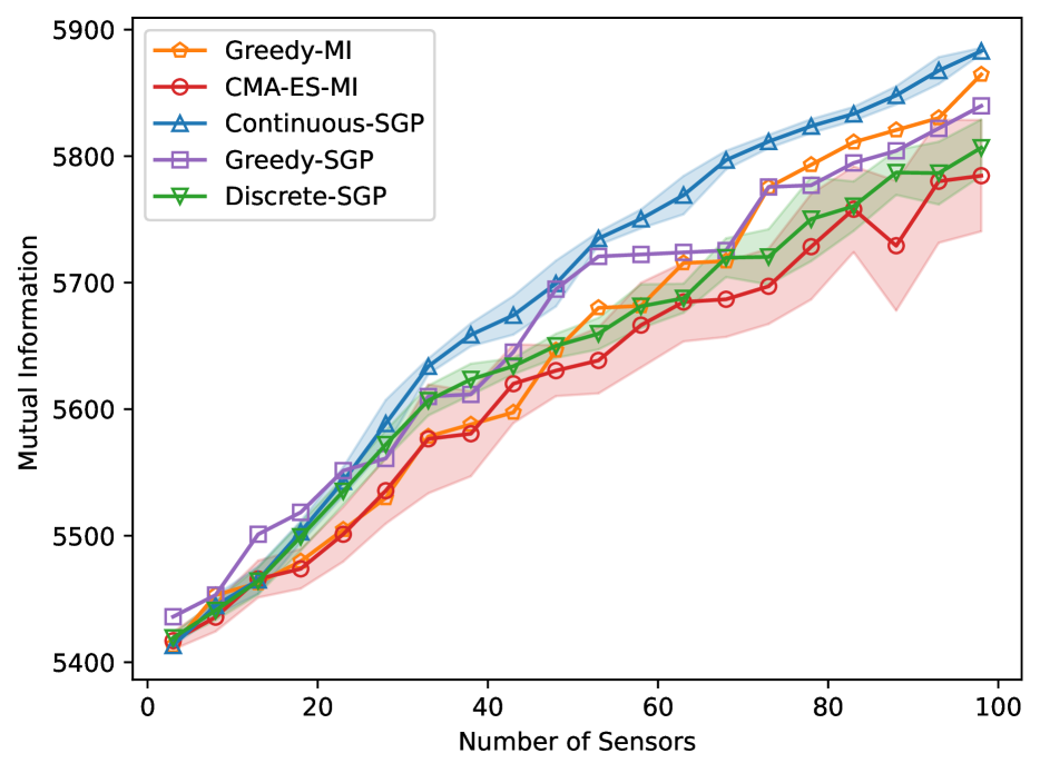
(a) Soil dataset MI

(b) Soil dataset ELBO

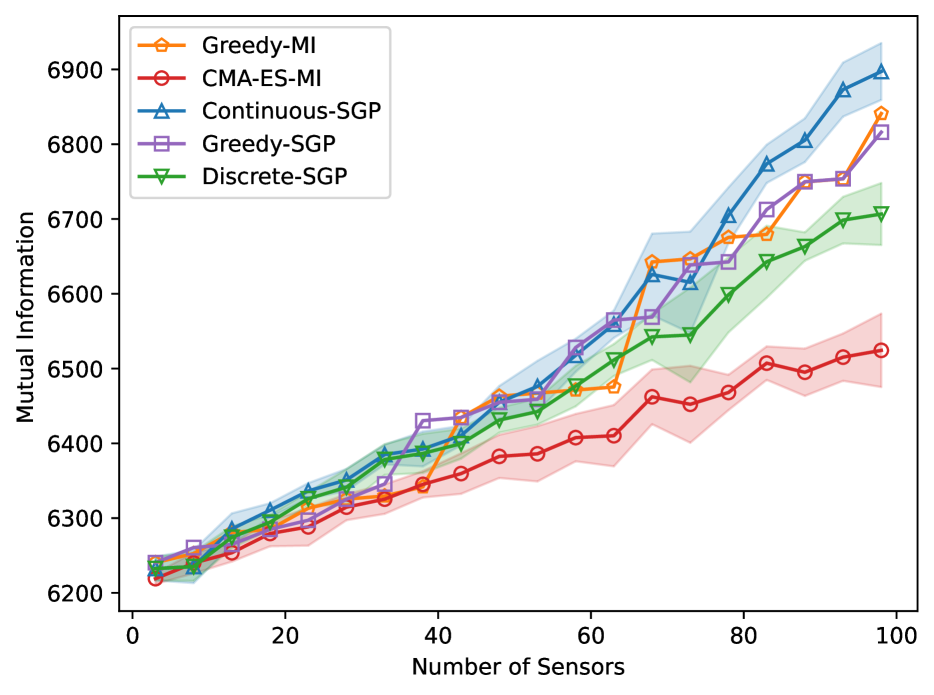
(c) Salinity dataset MI

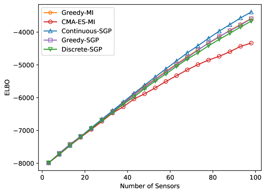
(d) Salinity dataset ELBO

Figure 3: Comparison of the MI and SVGP’s lower bound (ELBO) for the soil and salinity datasets. The mean and standard deviation of the MI vs number of sensors (a), (c) and SVGP’s lower bound (ELBO) vs number of sensors (b), (d).

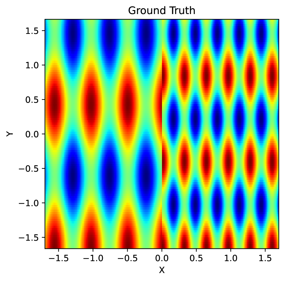
(a)

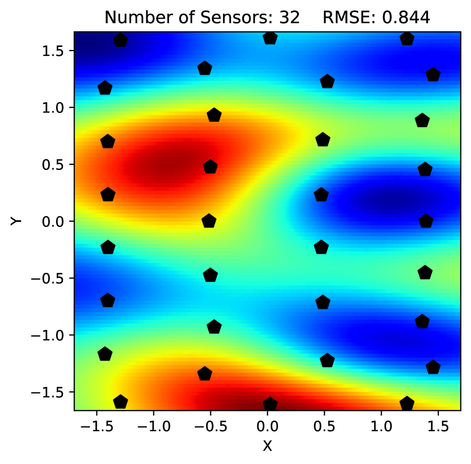
(b)

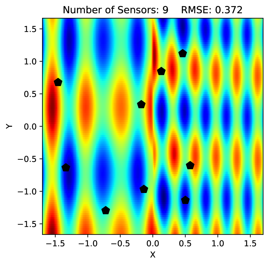
(c)

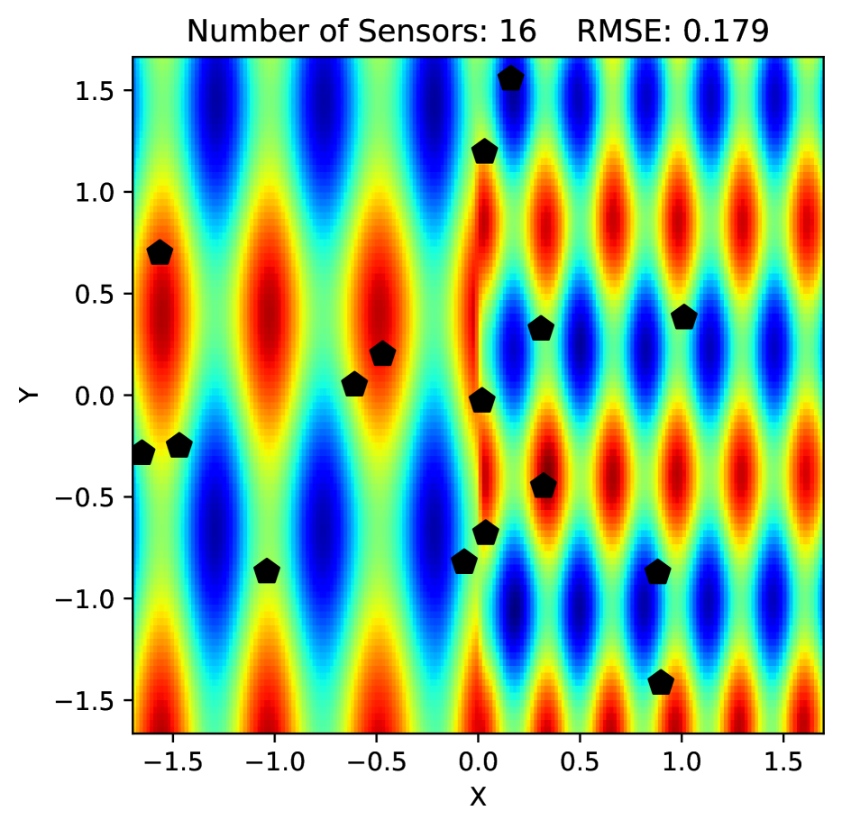
(d)

Figure 4: A non-stationary environment. (a) Ground truth. Reconstructions from the Continuous-SGP solutions for (b) 32 sensing locations with a stationary RBF kernel, and (c) 9 and (d) 16 sensing locations with the neural kernel. The black pentagons represent the solution placements.

We demonstrate our methods on four datasets—Intel lab temperature [Bodik et al., 2004], precipitation [Bretherton et al., 1999], soil moisture [Hain, 2013], and ROMS ocean salinity [Shchepetkin and McWilliams, 2005]. The datasets are representative of real-world sensor placement problems and some of these have been previously used as benchmarks [Krause et al., 2008]. We used an RBF kernel [Rasmussen and Williams, 2005] in these experiments.

The Intel lab temperature dataset contains indoor temperature data collected from 54 sensors deployed in the Intel Berkeley Research lab. The precipitation dataset contains daily precipitation data from 167 sensors around Oregon, U.S.A, in 1994. The US soil moisture dataset contains moisture readings from the continental USA, and the ROMS dataset contains salinity data from the Southern California Bight region. We uniform sampled 150 candidate sensor placement locations in the soil and salinity datasets.

For each dataset, we used a small portion of the data to learn the kernel parameters. and used a Gaussian process (GP) to reconstruct the data field in the environment from each method’s solution placements. The GP was initialized with the learned kernel function, and the solution sensing locations and their corresponding ground truth labels were used as the training set in the GP. We evaluated our data field reconstructions using the root-mean-square error (RMSE).

We benchmarked our approaches—Continuous-SGP (Section 5.1), Greedy-SGP (Section 5.2), and Discrete-SGP (Section 5.3). We also evaluated the performance of the approach in [Krause et al., 2008], which maximizes mutual information (MI) using the greedy algorithm (Greedy-MI) in discrete environments, and we used the covariance matrix adaptation evolution strategy (CMA-ES) to maximize MI (CMA-ES-MI) as another baseline as it can handle continuous environments. We chose these baselines as they have also been show to perform well on sensor placement problems. All methods considered the sparsely labeled sensor placement problem, i.e., only a small portion of labeled data was available to learn the kernel parameters.

We computed the solution sensor placements for 3 to 100 sensors (in increments of 5) for all the datasets, except for the Intel dataset, which was tested for up to 30 placement locations since it has only 54 placement locations in total. The experiments were repeated 10 times and we report the mean and standard deviation of the RMSE and runtime results in Figures 1 and 2. We see that our approaches’ RMSE results are consistently on par or better that the baseline Greedy-MI and CMA-ES-MI approaches.

Moreover, our approaches are substantially faster than the baseline approaches. Our Continuous-SGP approach is up to $6$ times faster than the baselines in the temperature dataset, up to $50$ times faster in the precipitation dataset, and up to $43$ times faster in the soil and salinity datasets. Our SGP-based approaches select sensing locations that reduce the RMSE by maximizing the SGP’s ELBO, which requires inverting only an $m\times m$ covariance matrix ($m\ll|\mathcal{S}|$, where $|\mathcal{S}|$ is the number of candidate locations). In contrast, both the baselines maximize MI, which requires inverting up to an $|\mathcal{S}|\times|\mathcal{S}|$ covariance matrix to place each sensor, which takes $\mathcal{O}(|\mathcal{S}|^{3})$ time. As such, the computational cost difference is further exacerbated in the precipitation, soil, and salinity datasets, which have three times as many candidate locations as the temperature data.

Also, the Continuous-SGP method consistently generates high quality results in our experiments; which is consistent with the findings of [Bauer et al., 2016], who showed that SVGP’s are able to recover the full GP posterior in regression tasks. Solving the assignment problem in our Discrete-SGP approach to map the Continuous-SGP solution to the discrete candidate set incurs a one-time $\mathcal{O}(m^{3})$ computation time that is negligible. Therefore our gradient-based approaches—Continuous-SGP and Discrete-SGP—converge at almost the same rate. Yet the Discrete-SGP retains the solution quality of the Continuous-SGP solution.

The labeled data locations in the soil and salinity datasets used to train our kernel function were not aligned with our candidate locations for the discrete approaches. We chose this setup to demonstrate that we can learn the kernel parameters even if the data is not aligned with the candidate locations, or is from a different environment altogether.

In Figure 3 we show the MI and SVGP’s lower bound (ELBO) between the solution placements and the environments (2500 uniformly sampled locations). The label dependent data fit term in the ELBO was disabled to generate the shown results. Although the ELBO values differ from MI, they closely approximate the relative trends of the MI values. This validates our claim that the SVGP’s ELBO behaves similarly to MI while being significantly cheaper to compute.

When using stationary kernels, our approach and approaches that maximize MI generate solution placements that are equally spaced. However, the solution placements are more informative when using non-stationary kernels. The following experiment demonstrates our approach in a non-stationary environment. We used a neural kernel [Remes et al., 2018] to learn the non-stationary correlations in the environment (Figure 4). We see that our placements from the SGP approach with the neural kernel are not uniformly distributed and are able to achieve near-perfect reconstructions of the environment. Please refer to the Supplementary for further details and experiments.

8 Conclusion

We addressed the sensor placement problem for monitoring correlated data. We formulated the problem as a regression problem using SGPs and showed that training SGPs on unlabeled data gives us ideal sensor placements in continuous spaces, thereby opening up the vast GP and SGP literature to the sensor placement problem and its variants involving constraints, non-point sensors, etc. The method also enables us to leverage the convergence rate proofs of SGPs. Furthermore, we presented an approach that uses the assignment problem to map the continuous domain solutions to discrete domains efficiently, giving us computationally efficient discrete solutions compared to the greedy approach. Our experiments on four real-world datasets demonstrated that our approaches result in both MI and reconstruction quality being on par or better than the existing approaches while substantially reducing the computation time.

A key advantage of our approach is its differentiability with respect to the sensing locations. We leverage this property in concurrent work to generalize our sensor placement approach to robotic informative path planning. Since GP-based approaches rely on having accurate kernel function parameters, we aim to develop online approaches to address this in our future work.

References

- [Bai et al., 2006] Bai, X., Kumar, S., Xuan, D., Yun, Z., and Lai, T. H. (2006). Deploying Wireless Sensors to Achieve Both Coverage and Connectivity. In Proceedings of the 7th ACM International Symposium on Mobile Ad Hoc Networking and Computing, page 131–142, New York, NY, USA.
- [Bauer et al., 2016] Bauer, M., van der Wilk, M., and Rasmussen, C. E. (2016). Understanding Probabilistic Sparse Gaussian Process Approximations. In Advances in Neural Information Processing Systems, page 1533–1541, Red Hook, NY, USA.
- [Bishop, 2006] Bishop, C. (2006). Pattern Recognition and Machine Learning. Springer, New York.
- [Bodik et al., 2004] Bodik, P., Hong, W., Guestrin, C., Madden, S., Paskin, M., and Thibaux, R. (2004). Intel lab data. Online dataset.
- [Breitenmoser et al., 2010] Breitenmoser, A., Schwager, M., Metzger, J.-C., Siegwart, R., and Rus, D. (2010). Voronoi coverage of non-convex environments with a group of networked robots. In 2010 IEEE International Conference on Robotics and Automation, pages 4982–4989.
- [Bretherton et al., 1999] Bretherton, C., Widmann, M., Dymnikov, V., Wallace, J., and Bladé, I. (1999). The effective number of spatial degrees of freedom of a time-varying field. Journal of Climate, 12(7):1990–2009.
- [Bui et al., 2017] Bui, T. D., Yan, J., and Turner, R. E. (2017). A Unifying Framework for Gaussian Process Pseudo-Point Approximations Using Power Expectation Propagation. Journal of Machine Learning Research, 18(104):1–72.
- [Buisson-Fenet et al., 2020] Buisson-Fenet, M., Solowjow, F., and Trimpe, S. (2020). Actively Learning Gaussian Process Dynamics. In Bayen, A. M., Jadbabaie, A., Pappas, G., Parrilo, P. A., Recht, B., Tomlin, C., and Zeilinger, M., editors, Proceedings of the 2nd Conference on Learning for Dynamics and Control, volume 120 of Proceedings of Machine Learning Research, pages 5–15. PMLR.
- [Burkard et al., 2012] Burkard, R., Dell’Amico, M., and Martello, S. (2012). Assignment Problems: revised reprint. SIAM, Philadelphia, USA.
- [Burt et al., 2019] Burt, D., Rasmussen, C. E., and Van Der Wilk, M. (2019). Rates of Convergence for Sparse Variational Gaussian Process Regression. In Chaudhuri, K. and Salakhutdinov, R., editors, Proceedings of the 36th International Conference on Machine Learning, volume 97, pages 862–871. PMLR.
- [Cortes et al., 2004] Cortes, J., Martinez, S., Karatas, T., and Bullo, F. (2004). Coverage control for mobile sensing networks. IEEE Transactions on Robotics and Automation, 20(2):243–255.
- [de Berg et al., 2008] de Berg, M., Cheong, O., van Kreveld, M., and Overmars, M. (2008). Computational Geometry: Algorithms and Applications. Springer-Verlag, Berlin, third edition.
- [Francis et al., 2019] Francis, G., Ott, L., Marchant, R., and Ramos, F. (2019). Occupancy map building through Bayesian exploration. The International Journal of Robotics Research, 38(7):769–792.
- [Hain, 2013] Hain, C. (2013). NASA SPoRT-LiS Soil Moisture Products.
- [Hamelijnck et al., 2021] Hamelijnck, O., Wilkinson, W. J., Loppi, N. A., Solin, A., and Damoulas, T. (2021). Spatio-Temporal Variational Gaussian Processes. In Beygelzimer, A., Dauphin, Y., Liang, P., and Vaughan, J. W., editors, Advances in Neural Information Processing Systems.
- [Hensman et al., 2013] Hensman, J., Fusi, N., and Lawrence, N. D. (2013). Gaussian Processes for Big Data. In Proceedings of the Twenty-Ninth Conference on Uncertainty in Artificial Intelligence, page 282–290, Arlington, Virginia, USA. AUAI Press.
- [Hitz et al., 2017] Hitz, G., Galceran, E., Garneau, M.-E., Pomerleau, F., and Siegwart, R. (2017). Adaptive Continuous-Space Informative Path Planning for Online Environmental Monitoring. Journal of Field Robotics, 34(8):1427–1449.
- [Hoang et al., 2015] Hoang, T. N., Hoang, Q. M., and Low, B. K. H. (2015). A Unifying Framework of Anytime Sparse Gaussian Process Regression Models with Stochastic Variational Inference for Big Data. In Bach, F. and Blei, D., editors, Proceedings of the 32nd International Conference on Machine Learning, volume 37, pages 569–578, Lille, France. PMLR.
- [Husain and Caselton, 1980] Husain, T. and Caselton, W. F. (1980). Hydrologic Network Design Methods and Shannon’s Information Theory. IFAC Proceedings Volumes, 13(3):259–267. IFAC Symposium on Water and Related Land Resource Systems, Cleveland, OH, USA, May 1980.
- [Jakkala and Akella, 2022] Jakkala, K. and Akella, S. (2022). Probabilistic Gas Leak Rate Estimation Using Submodular Function Maximization With Routing Constraints. IEEE Robotics and Automation Letters, 7(2):5230–5237.
- [Krause et al., 2008] Krause, A., Singh, A., and Guestrin, C. (2008). Near-Optimal Sensor Placements in Gaussian Processes: Theory, Efficient Algorithms and Empirical Studies. Journal of Machine Learning Research, 9(8):235–284.
- [Ma et al., 2017] Ma, K.-C., Liu, L., and Sukhatme, G. S. (2017). Informative Planning and Online Learning with Sparse Gaussian Processes. In 2017 IEEE International Conference on Robotics and Automation (ICRA), pages 4292–4298.
- [Quinonero-Candela et al., 2007] Quinonero-Candela, J., Rasmussen, C. E., and Williams, C. K. I. (2007). Approximation Methods for Gaussian Process Regression. In Large-Scale Kernel Machines, pages 203–223. MIT Press.
- [Ramsden, 2009] Ramsden, D. (2009). Optimization approaches to sensor placement problems. PhD thesis, Department of Mathematical Sciences, Rensselaer Polytechnic Institute.
- [Rasmussen and Williams, 2005] Rasmussen, C. E. and Williams, C. K. I. (2005). Gaussian Processes for Machine Learning. MIT Press, Cambridge, USA.
- [Remes et al., 2018] Remes, S., Heinonen, M., and Kaski, S. (2018). Neural non-stationary spectral kernel. ArXiv.
- [Sadeghi et al., 2022] Sadeghi, A., Asghar, A. B., and Smith, S. L. (2022). Distributed multi-robot coverage control of non-convex environments with guarantees. IEEE Transactions on Control of Network Systems, pages 1–12.
- [Salam and Hsieh, 2019] Salam, T. and Hsieh, M. A. (2019). Adaptive sampling and reduced-order modeling of dynamic processes by robot teams. IEEE Robotics and Automation Letters, 4(2):477–484.
- [Schwager et al., 2017] Schwager, M., Vitus, M. P., Powers, S., Rus, D., and Tomlin, C. J. (2017). Robust adaptive coverage control for robotic sensor networks. IEEE Transactions on Control of Network Systems, 4(3):462–476.
- [Shchepetkin and McWilliams, 2005] Shchepetkin, A. F. and McWilliams, J. C. (2005). The regional oceanic modeling system (ROMS): a split-explicit, free-surface, topography-following-coordinate oceanic model. Ocean Modelling, 9(4):347–404.
- [Shewry and Wynn, 1987] Shewry, M. C. and Wynn, H. P. (1987). Maximum entropy sampling. Journal of Applied Statistics, 14(2):165–170.
- [Snelson and Ghahramani, 2006] Snelson, E. and Ghahramani, Z. (2006). Sparse Gaussian Processes using Pseudo-inputs. In Weiss, Y., Schölkopf, B., and Platt, J., editors, Advances in Neural Information Processing Systems, volume 18. MIT Press.
- [Suryan and Tokekar, 2020] Suryan, V. and Tokekar, P. (2020). Learning a Spatial Field in Minimum Time With a Team of Robots. IEEE Transactions on Robotics, 36(5):1562–1576.
- [Titsias, 2009] Titsias, M. (2009). Variational Learning of Inducing Variables in Sparse Gaussian Processes. In van Dyk, D. and Welling, M., editors, Proceedings of the Twelth International Conference on Artificial Intelligence and Statistics, pages 567–574, Florida, USA. PMLR.
- [Whitman et al., 2021] Whitman, J., Maske, H., Kingravi, H. A., and Chowdhary, G. (2021). Evolving Gaussian Processes and Kernel Observers for Learning and Control in Spatiotemporally Varying Domains: With Applications in Agriculture, Weather Monitoring, and Fluid Dynamics. IEEE Control Systems, 41:30–69.
- [Wilkinson et al., 2021] Wilkinson, W. J., Särkkä, S., and Solin, A. (2021). Bayes-Newton Methods for Approximate Bayesian Inference with PSD Guarantees. CoRR, abs/2111.01721.
- [Wu and Zidek, 1992] Wu, S. and Zidek, J. V. (1992). An entropy-based analysis of data from selected NADP/NTN network sites for 1983–1986. Atmospheric Environment. Part A. General Topics, 26(11):2089–2103.
- [Zhu et al., 2021] Zhu, H., Chung, J. J., Lawrance, N. R., Siegwart, R., and Alonso-Mora, J. (2021). Online Informative Path Planning for Active Information Gathering of a 3D Surface. In 2021 IEEE International Conference on Robotics and Automation (ICRA), pages 1488–1494.