Monitoring of the polarized H₂O maser emission around the massive protostars W75N(B)-VLA 1 and W75N(B)-VLA 2.

Abstract

Context. Several radio sources have been detected in the high-mass star-forming region W75N(B), among them the massive young stellar objects VLA 1 and VLA 2 are of great interest. These are thought to be in different evolutionary stages. In particular, VLA 1 is at the early stage of the photoionization and it is driving a thermal radio jet, while VLA 2 is a thermal, collimated ionized wind surrounded by a dusty disk or envelope. In both sources 22 GHz H₂O masers have been detected in the past. Those around VLA 1 show a persistent linear distribution along the thermal radio jet and those around VLA 2 have instead traced the evolution from a non-collimated to a collimated outflow over a period of $\sim$20 years. The magnetic field inferred from the H₂O masers showed an orientation rotation following the direction of the major-axis of the shell around VLA 2, while it is immutable around VLA 1.

Aims. By monitoring the polarized emission of the 22 GHz H₂O masers around both VLA 1 and VLA 2 over a period of six years, we aim to determine whether the H₂O maser distributions show any variation over time and whether the magnetic field behaves accordingly.

Methods. The European VLBI Network was used in full polarization and phase-reference mode in order to determine the absolute positions of the 22 GHz H₂O masers with a beam size of $\sim 1$ mas and to determine both the orientation and the strength of the magnetic field. We observed four epochs separated by two years from 2014 to 2020.

Results. We detected polarized emission from the H₂O masers around both VLA 1 and VLA 2 in all the epochs. By comparing the H₂O masers detected in the four epochs, we find that the masers around VLA 1 are tracing a nondissociative shock originating from the expansion of the thermal radio jet, while the masers around VLA 2 are tracing an asymmetric expansion of the gas that is halted in the northeast where the gas likely encounters a very dense medium. We also found that the magnetic field inferred from the H₂O masers in each epoch can be considered as a portion of a quasi-static magnetic field estimated in that location rather than in that time. This allowed us to study locally the morphology of the magnetic field around both VLA 1 and VLA 2 in a larger area by considering the vectors estimated in all the epochs as a whole. We find that the magnetic field in VLA 1 is along the jet axis and bends toward north and south at the northeast and southwest ends of the jet, respectively, reconnecting with the large-scale magnetic field. The magnetic field in VLA 2 is perpendicular to the expansion directions till it encounters the denser matter in the northeast, here the magnetic field is parallel to the expansion direction and agrees with the large-scale magnetic field. We also measured the magnetic field strength along the line of sight in three of the four epochs, whose values are $-764\leavevmode\nobreak\ \rm{mG}<B_{\rm{||}}^{\rm{VLA\,1}}<-676$ mG and $-355\leavevmode\nobreak\ \rm{mG}<B_{\rm{||}}^{\rm{VLA\,2}}<-2426$ mG.

1 Introduction

All stars in the sky are generally divided into two main groups according to their mass: low-mass stars ($M<8$ M_⊙) and high-mass stars ($M>8$ M_⊙). While for the first group the formation process is quite well established, for the high-mass stars there are still several open questions that need to be addressed (e.g., Tan et al. 2014; Motte et al. 2018). However, based on observational constraints, an evolutionary scenario of high-mass star formation (HMSF) was proposed by Motte et al. (2018). This is summarized in the following. High-mass stars form in molecular complexes, in particular in parsec-scale massive clumps/clouds that first undergo a global controlled collapse forming low-mass prestellar cores. This first phase is known as starless massive dense cores (MDCs). After about 10⁴ years, low-mass prestellar cores become protostars with growing mass. This phase is called protostellar MDC phase. Only after $\sim 10^{5}$ years more we have the high-mass protostellar phase where, thanks to the gas flow streams generated by the global collapse, the protostars become high-mass protostars, even though they still harbor low-mass stellar embryos. At this stage of the evolution the high-mass protostars are still quiet in the infrared (IR) and if their accretion rates are efficient and strong they drive outflows. In this phase the accretion disks are already formed. As soon as the stellar embryos reach more than 8 M_⊙ the high-mass protostars become IR-bright and they develop ultra-compact H ii region (UCH ii) that are quenched by infalling gas or confined to the photoevaporating disks. Finally, we have the H ii region phase that lasts about $10^{5}-10^{6}$ years. In this phase, the ultraviolet radiation from the stellar embryos produces the H ii region and the gas accretion toward the newborn star first slows down and then stops by terminating the main accretion phase. The high-mass star is formed.
The great importance that the magnetic field has in several phases of HMSF has been showed through magnetohydrodynamical (MHD) simulations (e.g., Myers et al. 2014; Kuiper et al. 2016; Matsushita et al. 2018; Machida & Hosokawa 2020; Rosen & Krumholz 2020; Oliva & Kuiper 2022). Despite the observational difficulties, which are due to the low number of high-mass protostars that are usually found densely clustered in molecular clouds and to their long distances to the Sun, measurements of the morphology and strength of magnetic fields close to high-mass protostars are possible. These can be obtained by observing the polarized emission of dust and molecular lines with the Atacama Large Millimeter Array (ALMA; e.g., Dall’Olio et al. 2019; Sanhueza et al. 2021), and by observing the polarized maser emission with the very long baseline interferometry (VLBI) technique (e.g., Surcis et al. 2011a, b, 2014, 2022). A relevant star-forming region where it is possible to measure the magnetic field close to high-mass young stellar objects (YSOs) in different evolutionary phases is W75N(B).
The active high-mass star-forming region (HMSFR) W75N is part of the Cygnus X complex (Westerhout 1958; Harvey et al. 1977; Habing & Israel 1979) at a distance of 1.30$\pm$0.07 kpc (Rygl et al. 2012). Haschick et al. (1981) identified three compact radio regions within W75N at a spatial resolution of $\sim 1^{\prime\prime}\!\!.5$: W75N(A), W75N(B), and W75N(C). In 1994, Hunter et al. further mapped the continuum emission of W75N(B) at a resolution of $\sim 0^{\prime\prime}\!\!.5$ revealing the presence of three very compact subregions (Ba, Bb, and Bc). For the first time Hunter et al. (1994) also underlined the great importance of the region for understanding the star formation process thanks to its significant activity. The subregions Ba and Bb were renamed as VLA 1 and VLA 3 in 1997 when Torrelles et al. (1997) imaged them at a resolution of $\sim 0^{\prime\prime}\!\!.1$ with the Very Large Array (VLA). Torrelles et al. (1997) also imaged for the first time another weaker and more compact radio source between VLA 1 and VLA 3, called VLA 2. While VLA 1 and VLA 3 showed a well elongated radio continuum emission along northeast-southwest and northwest-southeast directions, respectively, that were consistent with the morphology of thermal radio jets, VLA 2 showed a quasi-circular morphology that was supposed to be an UCH ii. Despite their small separation (VLA 2 is only $\sim 0^{\prime\prime}\!\!.8$, $\sim 1000$ au at 1.3 kpc, from VLA 1), the three radio sources are thought to be massive YSOs (Shepherd et al. 2003) at three different evolutionary stages, with VLA 1 the most evolved and VLA 2 the least evolved (Torrelles et al. 1997). In addition, Shepherd et al. (2003) report a systemic velocity for W75N(B) of $V_{\rm{lsr}}=+10.0$ km s^-1, which can also be considered as the systemic velocity for VLA 1, VLA 2, and VLA 3. Five more new radio sources were identified in W75N(B) thanks to high sensitive observations made with the upgraded VLA. They are VLA 4, that is about $\sim 1^{\prime\prime}\!\!.5$ south of Bc (Carrasco-González et al. 2010), VLA [NE] ($\sim 8^{\prime\prime}$ northeast of VLA 2), VLA [SW] ($\sim 6^{\prime\prime}$ southwest of VLA 2), and Bd ($\sim 0.5^{\prime\prime}$ northeast of VLA 4; Rodríguez-Kamenetzky et al. 2020). Thanks to ALMA observations at 1.3 mm (spatial resolution of $\sim 1.2^{\prime\prime}$), Rodríguez-Kamenetzky et al. (2020) were able to associate VLA [NE] and VLA [SW] with the millimeter cores MM3 and MM2, respectively, indicating that they are also embedded YSOs. Furthermore, VLA 1, VLA 2, and VLA 3 are also associated with a millimeter core (MM1) but VLA 4, Bc, and Bd are not, which suggests that they are not embedded YSOs but shock-ionized gas (Rodríguez-Kamenetzky et al. 2020). In addition, the multi wavelength observations made by Carrasco-González et al. (2015) with the VLA showed that VLA 2 changed its morphology between 1996 and 2014 from a compact roundish source ($\leq 160$ au; Torrelles et al. 1997) to an extended source that is elongated in the northeast-southwest direction ($220\times\leq 160$ au, position angle of PA=65^∘), while VLA 1 still shows an unchanged morphology since 1996 (Rodríguez-Kamenetzky et al. 2020). The spectral index analysis indicates that VLA 2 is a thermal, collimated ionized wind surrounded by a dusty disk or envelope (Carrasco-González et al. 2015), VLA 1 is at the early stage of the photoionization and it is driving a thermal radio jet, and VLA 3 is also driving a thermal radio jet whose shocks are traced by the obscured Herbig-Haro (HH) objects Bc and VLA 4 (Rodríguez-Kamenetzky et al. 2020).
A large-scale high-velocity CO-outflow, with an extension greater than 3 pc (PA=66^∘) and with a total molecular mass greater than 255 M_⊙, was detected from W75N(B) (e.g., Hunter et al. 1994; Davis et al. 1998; Shepherd et al. 2003; Makin & Froebrich 2018). Shepherd et al. (2003) found that the entire CO emission of W75N uncovers a complex morphology of multiple, overlapping outflows. In particular, they suggest that VLA 2 may drive the large-scale CO-outflow, while VLA 1 and VLA 3 are instead the centers of two additional, more compact outflows (extension of $\sim$0.21 pc and $\sim$0.15 pc, respectively). However, this is not clear yet and the main powering source of the large-scale CO-outflow remains undetermined (e.g., Qiu et al. 2008). In addition, Shepherd et al. (2003) also determined that more than 10% of the molecular gas in W75N is outflowing material, and the combined outflow energy is roughly half the gravitational binding energy of the cloud thus preventing its further collapse.

Table 1: Observational details.

(1)	(2)	(3)	(4)	(5)	(6)	(7)	(8)	(9)	(10)	(11)	(12)
Observation	Antennas	Bandwidth	Spectral	Source	Restoring	Position	Peak	rms	$\sigma_{\rm{s.-n.}}$	$P_{\rm{l}}$	Polarization
date			channels	name	Beam size	Angle	intensity (I)				angle
		(MHz)			(mas $\times$ mas)	(∘)	($\frac{\rm{Jy}}{\rm{beam}}$)	($\frac{\rm{mJy}}{\rm{beam}}$)	($\frac{\rm{mJy}}{\rm{beam}}$)	(%)	(∘)
17 June 2014	Ef, On, Nt, Tr, Ys, Mh	4	2048	W75N(B)	$1.1\times 0.8$	$-60.02$	-	13	25	-	-
				J2040+4527	$1.1\times 0.7$	$-62.40$	0.029	0.6	-	-	-
				J2202+4216	$1.5\times 0.8$	$-52.68$	1.868	2.5	-	7.0	$-64\pm 8$
12 June 2016	Ef, Jb, Mc, Nt, Sr, Ys,	4	2048	W75N(B)	$1.9\times 1.2$	$-86.02$	-	11	73	-	-
	Mh			J2040+4527	$1.0\times 0.7$	$-86.84$	0.026	0.7	-	-	-
				J2202+4216	$1.5\times 1.0$	$+74.56$	0.685	1.5	-	3.1	$-61\pm 12$
				3C48	$1.5\times 0.9$	$-59.93$	0.016	1.1	-	¡21	$-$
09 June 2018	Ef, Jb, Mc, On, Nt, Tr,	8	4096	W75N(B)	$1.2\times 1.0$	$+86.92$	-	14	28	-	-
	Sr, Ys, Mh			J2040+4527	$1.1\times 0.8$	$-79.82$	0.021	0.4	-	-	-
				J2202+4216	$1.2\times 0.8$	$-61.91$	0.765	1.7	-	4.0	$+5\pm 1$
				3C48	$1.8\times 0.7$	$-42.47$	0.125	0.5	-	4.2	$-70\pm 1$
25 Oct. 2020	Ef, Jb, Mc, On, Tr, Sr,	8	4096	W75N(B)	$1.4\times 1.0$	$-53.96$	-	13	12	-	-
	Ys, Mh			J2040+4527	$1.3\times 0.9$	$-56.63$	0.034	0.6	-	-	-
				J2202+4216	$1.6\times 1.0$	$-75.93$	1.011	2.2	-	3.8	$+15\pm 1$
				3C48	$2.2\times 1.1$	$-38.84$	0.027	0.3	-	6.4	$-70\pm 1$

The great interest that W75N(B) has aroused in the past is also due to the presence of several maser species (OH, CH₃OH, and H₂O) around the two sources VLA 1 and VLA 2 (e.g., Haschick et al. 1981; Hunter et al. 1994; Torrelles et al. 1997; Lekht & Krasnov 2000; Minier et al. 2000; Surcis et al. 2009; Fish et al. 2011; Kang et al. 2016; Colom et al. 2018, 2021). OH masers are distributed throughout the region with the majority of the maser spots associated with VLA 1 (Hutawarakorn et al. 2002; Fish et al. 2005). Nevertheless, VLA 2 is the site of the most intensive OH flare ever registered in a star-forming region (1000 Jy, Alakoz et al. 2005; Slysh et al. 2010), while other OH maser emission sites are situated on a ring structure around VLA 1, VLA 2, and VLA 3 (Hutawarakorn et al. 2002). In 2011, Fish et al. measured the proper motions of the OH masers showing that most of those near VLA 1 (located $\sim 1^{\prime\prime}$ northwest) are moving northward ($V<+5$ km s^-1) and those associated with VLA 2, and located southwest, are moving both toward southwest and southeast ($V<+5$ km s^-1). The detection of OH maser Zeeman-pairs provided measurements of magnetic field strength between 6 and 8 mG close to VLA 1, where the 22 GHz H₂O maser are detected, and up to about 17 mG around VLA 2 (Fish et al. 2011). However, higher values (40-70 mG, Slysh & Migenes 2006; Slysh et al. 2010) were measured during the strong OH maser flare. The 6.7 GHz CH₃OH masers are only associated with VLA 1 and they are distributed parallel to the thermal radio jet of VLA 1 (Minier et al. 2000, 2001; Surcis et al. 2009). No CH₃OH masers were detected around VLA 2 (Surcis et al. 2009; Rygl et al. 2012) till 2014, when three maser spots were detected in the southwest of the source (Carrasco-González et al. 2015). Thanks to the polarized emission of the CH₃OH masers, Surcis et al. (2009) were able to measure a magnetic field oriented southwest - northeast, that is perfectly aligned with VLA 1, and whose strength on the line of the sight was found to be $|B_{||}|>10$ mG (Surcis et al. 2019).
The 22 GHz H₂O masers have been widely studied and monitored both with single dishes and interferometers, revealing a high intensity variations, with extreme maser flares (up to 10³ Jy), and important variation in the maser distribution (e.g., Lekht & Sorochenko 1984; Lekht 1994; Lekht & Krasnov 2000; Torrelles et al. 2003; Surcis et al. 2011a; Kim et al. 2013; Surcis et al. 2014; Krasnov et al. 2015; Kim & Kim 2018). The H₂O masers are associated with VLA 1 and VLA 2, and only one maser was associated with VLA 3 in 1996 (Torrelles et al. 1997), but it has never been detected again (e.g., Torrelles et al. 2003; Surcis et al. 2014). Over a period of 16 years, VLBI observations have showed that the evolution of the H₂O masers around VLA 1 and VLA 2, despite their close separation, is completely different. Whereas the H₂O masers around VLA 1 are always linearly distributed ($\rm{PA}\approx 43$^∘) along the thermal radio jet, those detected around VLA 2 are instead tracing an expanding shell (expanding velocity of $\sim$30 km s^-1, Surcis et al. 2014) that evolved from a quasi-circular (Torrelles et al. 2003; Surcis et al. 2011a) to an elliptical structure (Kim et al. 2013; Surcis et al. 2014) following the morphology change in the continuum emission observed by Carrasco-González et al. (2015). Therefore, in VLA 2 the H₂O masers might be tracing the evolution from a non-collimated to a collimated outflow (Surcis et al. 2014). Furthermore, Surcis et al. (2014) also showed that the magnetic field around VLA 1 has not changed from 2005 to 2012 and it is always oriented along the direction of the thermal radio jet. Whereas, the orientation of the magnetic field around VLA 2 changed in a way that is consistent with the new direction of the major-axis of the shell-like structure that is now aligned with the thermal radio jet of VLA 1.

Figure 1: Contour maps of the phase-reference calibrator J2040+4527 in the EVN epochs 2014.46, 2016.45, 2018.44, and 2020.82 from left to right, respectively. Contours are 4, 8, 16, and 32 times 0.6 mJy beam^-1. The restoring beam is overplotted on the bottom left corner of each panel (see Table 1).

Table 2: Absolute position of the reference maser feature.

(1)	(2)	(3)	(4)	(6)	(7)	(8)		(9)	(10)	(11)
epoch	Reference	$V_{\rm{lsr}}$	$\alpha_{2000}$	$\varepsilon_{\rm{rms}}$	$\varepsilon_{\rm{gauss}}^{\alpha}$	$\Delta\alpha$		$\delta_{2000}$	$\varepsilon_{\rm{gauss}}^{\delta}$	$\Delta\delta$
	maser
		(km/s)	($\rm{{}^{h}:\leavevmode\nobreak\ ^{m}:\leavevmode\nobreak\ ^{s}}$)	(mas)	(mas)	(mas)	(s)	($\rm{{}^{\circ}:\,^{\prime}:\,^{\prime\prime}}$)	(mas)	(′′)
2014.46	VLA1.1.15	10.45	20:38:36.43399	0.003	0.006	$\pm$0.9	$\pm$0.00008	+42:37:34.8710	0.04	$\pm$0.0009
2016.45	VLA1.2.07	10.92	20:38:36.43403	0.029	0.05	$\pm$1.2	$\pm$0.00011	+42:37:34.8667	0.04	$\pm$0.0010
2018.44	VLA1.3.04	8.63	20:38:36.43201	0.018	0.04	$\pm$0.9	$\pm$0.00008	+42:37:34.8588	0.03	$\pm$0.0009
2020.82	VLA1.4.05	9.87	20:38:36.43111	0.029	0.06	$\pm$1.0	$\pm$0.00009	+42:37:34.8794	0.05	$\pm$0.0009

The peculiarity of the H₂O maser shell expansion with the contemporary variation of the magnetic field around VLA 2, together with the presence of a close-by immutable VLA 1 source, made W75N(B) one of the most interesting case where to investigate the evolution of early massive YSOs. For this reason that we performed every two years VLBI monitoring observations of 22 GHz H₂O maser emission in full polarization mode from 2014 to 2020 for a total of four epochs. Here, we report in Sect. 3 the results of the monitoring observations, that are described in Sect. 2. We discuss the magnetic fields around VLA 1 and VLA 2 in Sect. 4, and we finally present a full picture of the two massive YSOs in Sect. 5.

Table 3: Comparison of 22 GHz H₂O maser parameters between epochs 2014.46, 2016.45, 2018.44, and 2020.82.

	VLA 1				VLA 2
	2014.46	2016.45	2018.44	2020.82	2014.46	2016.45	2018.44	2020.82
Number of maser features	28	20	20	10	43	37	44	39
$V_{\rm{lsr}}$ range (km s-1)	$[+7.9;+19.7]$	$[+2.7;+16.4]$	$[+7.8;+15.0]$	$[+8.8;+26.4]$	$[-11.6;+21.2]$	$[-15.6;+20.7]$	$[-15.9;+28.2]$	$[-1.0;+27.2]$
$I$ range (Jy beam-1)	$[0.43;1205.52]$	$[0.24;1619.87]$	$[2.08;446.25]$	$[0.14;302.47]$	$[0.21;31.70]$	$[0.23;90.99]$	$[0.04;128.02]$	$[0.05;285.16]$
$\langle\Delta v_{\rm{L}}\rangle$ (km s-1)	$1.3$	$1.1$	$1.0$	$1.7$	$0.7$	$0.7$	$0.7$	$0.7$
	Polarization
$P_{\rm{l}}$ range (%)	$[0.4;15.6]$	$[0.7;2.2]$	$[0.7;10.6]$	$[0.1;0.3]$	$[0.9;4.6]$	$[0.6;2.7]$	$[1.0;2.3]$	$[0.2;1.9]$
$P_{\rm{V}}$ range (%)	$-$	$3.5$	$1.6$	$-$	$-$	$[4.9;7.8]$	$[1.5;2.9]$	$1.3$
	Intrinsic characteristics
$\Delta V_{\rm{i}}$ range (km s-1)	$[0.4;4.2]$	$[3.8;4.3]$	$[0.4;3.9]$	$2.6$	$[1.6;1.9]$	$[0.4;4.2]$	$[0.8;3.6]$	$[2.6;3.8]$
$T_{\rm{b}}\Delta\Omega$ range (log K sr)	$[7.0;9.4]$	$[6.8;9.3]$	$[8.9;10.5]$	$10.6$	$[8.9;9.2]$	$[6.1;9.4]$	$[6.0;10.5]$	$[8.2;8.4]$
$\langle\Delta V_{\rm{i}}\rangle$ (km s-1)	$3.0^{+0.2}_{-0.3}$	$2.8^{+0.3}_{-0.2}$	$2.7^{+0.5}_{-1.4}$	$2.6^{+0.1}_{-0.3}$	$1.6^{+0.2}_{-0.2}$	$2.9^{+0.2}_{-0.2}$	$2.1^{+0.8}_{-0.4}$	$2.9^{+0.1}_{-0.4}$
$\langle T_{\rm{b}}\Delta\Omega\rangle$ (log K sr)	$8.7^{+0.8}_{-0.9}$	$8.7^{+1.2}_{-0.9}$	$9.1^{+0.6}_{-0.3}$	$10.5^{+0.1}_{-0.4}$	$9.2^{+0.3}_{-1.2}$	$9.1^{+0.4}_{-1.9}$	$11.0^{+0.1}_{-4.2}$	$8.3^{+0.8}_{-0.8}$
$T$ (K)	$3600^{+496}_{-684}$	$3136^{+708}_{-432}$	$2916^{+1180}_{-2240}$	$2704^{+212}_{-588}$	$1024^{+272}_{-240}$	$3364^{+480}_{-448}$	$1764^{+1600}_{-608}$	$3364^{+236}_{-864}$
$\Gamma+\Gamma_{\nu}$	$20$	$18$	$16$	$15$	$7$	$18$	$10$	$18$
	Magnetic field
$\chi$ range (∘)	$[-62;+48]$	$[-76;-11]$	$[-88;+88]$	$[-67;-5]$	$[-47;-31]$	$[-77;+88]$	$[-89;+90]$	$[-54;+40]$
$\theta$ range (∘)	$[+75;+90]$	$+90$	$[+62;+90]$	$[+5;+54]$	$[+79;+86]$	$[+76;+90]$	$[+14;+90]$	$[+66;+90]$
$\Phi_{\rm{B}}$ range (∘)	$[-42;+68]$	$[+14;+18]$	$[-4;+88]$	$[-5;-67]$	$[+43;+51]$	$[-3;+45]$	$[-25;+85]$	$[-64;+80]$
$|B_{||}|$ range (mG)	$-$	$676$	$[733;764]$	$-$	$-$	$[1498;2426]$	$[355;439]$	$452$
$\langle\chi\rangle$ (∘)	$-47\pm 30$	$-60\pm 16$	$-87\pm 5$	$-32\pm 44$	$-40\pm 7$	$-74\pm 19$	$+76\pm 12$	$-73\pm 62$
$\langle\theta\rangle$ (∘)	$90^{+21}_{-21}$	$90^{+19}_{-19}$	$+78^{+11}_{-11}$	$+55^{+2}_{-48}$	$86^{+3}_{-13}$	$90^{+18}_{-18}$	$90^{+37}_{-37}$	$90^{+49}_{-49}$
$\langle\Phi_{\rm{B}}\rangle$ (∘)	$+43\pm 30$	$+30\pm 16$	$-10\pm 36$	$-32\pm 44$	$+50\pm 7$	$+16\pm 19$	$-29\pm 36$	$+61\pm 31$
$\langle|B_{||}|\rangle$ (mG)	$-$	$676\pm 102$	$748\pm 22$	$-$	$-$	$1755\pm 656$	$399\pm 59$	$452\pm 68$
$\langle|B|\rangle$ (mG)	$-$	$>2076$	$3598\pm 106$	$-$	$-$	$>5679$	$>663$	$>598$
Arithmetic mean of $|B_{||}|$ (mG)	$-$	$676$	$748$	$-$	$-$	$1962$	$397$	$452$

2 Observations and analysis

W75N(B) was observed at 22 GHz in full polarization spectral mode with several European VLBI Network (EVN) antennas on four epochs separated by two years (see Table 1). The observations were carried out in June 2014 (epoch 2014.46), 2016 (epoch 2016.45), and 2018 (epoch 2018.44) and in October 2020 (epoch 2020.82), for a total observation time per epoch of 12 h. The bandwidth was 4 MHz in epochs 2014.46 and 2016.45, providing a local standard of rest velocity ($V_{\rm{lsr}}$) range of $\sim 55$ km s^-1 (after calibration ranging from $-15.7$ km s^-1 to $+31.7$ km s^-1), and 8 MHz in epochs 2018.44 and 2020.82 (after calibration ranging from $-30.3$ km s^-1 to $+48.1$ km s^-1). We observed with a bandwidth two times wider in the last two epochs to search for maser emission at velocities $<-15.7$ km s^-1, as indicated by the results obtained in epoch 2016.45 (see Sec. A.2 and Table 13). To measure the absolute positions of the H₂O masers, the observations were conducted in phase-reference mode (with cycles phase-calibrator – target of 45 sec – 45 sec). The phase-reference calibrator was J2040+4527 (separation $=2^{\circ}\!\!.856$). The data were correlated with the EVN software correlator (SFXC; Keimpema et al. 2015) at the Joint Institute for VLBI ERIC (JIVE) using 2048 channels in epochs 2014.46 and 2016.45, and 4096 channels in epochs 2018.44 and 2020.82, generating all 4 polarization combinations (RR, LL, RL, and LR) with a spectral resolution in all epochs of $\sim$2 kHz ($\sim$0.03 km s^-1).
The data were calibrated using the Astronomical Image Processing Software package (AIPS) by following the standard calibration procedure (e.g., Surcis et al. 2011a). Specifically, the bandpass, the delay, the phase, and the polarization calibration were performed in all epochs on the calibrator J2202+4216. Then we performed the fringe-fitting and the self-calibration on the brightest maser feature of each epoch (reference maser features VLA1.1.15, VLA1.2.07, VLA1.3.04, and VLA1.4.05 in Tables 10, 12, 14, and 16, respectively; for the notation definition see Sect. 3). The I, Q, U, and V Stokes cubes were then imaged using the AIPS task IMAGR. Afterward, the Q and U cubes were combined to produce cubes of linearly polarized intensity ($POLC=\sqrt{Q^{2}+U^{2}-\sigma_{P}^{2}}$) and polarization angle ($POLA=1/2\times\leavevmode\nobreak\ atan(U/Q)$). The polarized intensity cubes were corrected according to the noise $\sigma_{P}=\sqrt{[(Q\times\sigma_{Q})^{2}+(U\times\sigma_{U})^{2}]/(Q^{2}+U^{2})}$, where $\sigma_{Q}$ and $\sigma_{U}$ are the noise of the Q and U Stokes cubes, respectively. The formal error on $POLA$ due to the thermal noise is given by $\sigma_{POLA}=0.5\leavevmode\nobreak\ (\sigma_{P}/POLC)\times(180^{\circ}/\pi)$ (Wardle & Kronberg 1974).
To measure the absolute positions of the H₂O maser features, we self-calibrated, in all four epochs, the phase-reference source J2040+4527 and the amplitude and phase solutions were applied only to the uncalibrated peak channel of the brightest maser feature of each epoch. We show the contours maps of J2040+4527 in Fig.1 and the absolute positions, with their uncertainties, of the reference maser feature of each epoch are listed in Table 2. The uncertainties of the absolute positions of the reference maser features are estimated by adding quadratically the systematic errors ($\varepsilon_{sys}=0.028$ mas) due to the source elevation limit and the separation between the calibrator and the target (Reid & Honma 2014, maximum and minimum elevation of W75N(B) at each station and in all epochs were $\sim 80$^∘ and $\sim 35$^∘, respectively), the errors due to the thermal noise ($\varepsilon_{\rm{rms}}$), the errors of the Gaussian fit of the peak spot of the reference maser feature ($\varepsilon_{\rm{gauss}}$), and the errors of $\alpha_{2000}$ and $\delta_{2000}$ of J2040+4527 (0.68 mas and 0.80 mas, respectively, Petrov et al. 2011). The later is usually unnecessary in relative astrometry studies, as the one presented here, however due to the large time interval between the EVN epochs we include it in our analysis to account for possible variation of the calibrator position from one epoch to the others. Another source of uncertainty that is taken into consideration here is that due to the identification of the maser features, that is to account for the maser spots scatter of each maser features (see Surcis et al. 2011a, hereafter S+11a), and it is equal to half of the restoring beam of W75N(B).

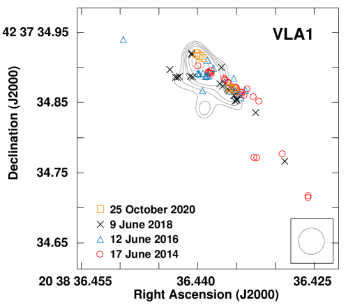
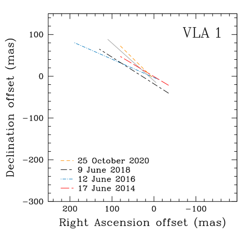
Figure 2: Comparison of the H₂O maser features detected toward VLA 1 (left panel) in the four EVN epochs (2014.46, 2016.45, 2018.44, and 2020.82) and superimposed to the uniform-weighted continuum map at Q-band (central frequency 44 GHz) of the thermal radio jet driven by VLA 1 obtained with the VLA by Rodríguez-Kamenetzky et al. (2020). The light gray contours are 5, 6, 7, 8, 10, 12, 14 times $\sigma=100\leavevmode\nobreak\ \rm{\mu Jy\leavevmode\nobreak\ beam^{-1}}$ and the VLA beam is shown on the bottom right corner. The positions of the maser features are corrected assuming the proper motion of the region W75N(B) equal to the median proper motion measured for the 6.7 GHz CH₃OH maser features by Rygl et al. (2012), $\langle\mu_{\rm{\alpha}}\rangle=(-1.97\pm 0.10)\leavevmode\nobreak\ \rm{mas\leavevmode\nobreak\ yr^{-1}}$ and $\langle\mu_{\rm\delta}\rangle=(-4.16\pm 0.15)\leavevmode\nobreak\ \rm{mas\leavevmode\nobreak\ yr^{-1}}$. In addition, the positions of the maser features associated with VLA 1 and detected in the last three epochs have been further corrected considering the proper motion of VLA 1 within W75N(B). This proper motion is $\langle\mu_{\rm{\alpha}}\rangle^{\rm{VLA\,1}}=(-6.3\pm 0.4)\leavevmode\nobreak\ \rm{mas\leavevmode\nobreak\ yr^{-1}}$ and $\langle\mu_{\rm\delta}\rangle^{\rm{VLA\,1}}=(+5.0\pm 0.4)\leavevmode\nobreak\ \rm{mas\leavevmode\nobreak\ yr^{-1}}$ (see Appendix B). The size of the symbols are ten times the uncertainties of the absolute positions of the maser features (see Table 2). For clarity we show in the right panel the linear fit of the maser features for each epoch, the length of the segments correspond to the position of the maser features used in the fitting. The reference position is $\alpha_{2000}=20^{\rm{h}}38^{\rm{m}}36^{\rm{s}}\!.43399$ and $\delta_{2000}=+42^{\circ}37^{\prime}34^{\prime\prime}\!\!.8710$. The parameters of the linear fit are reported in Table 6. The solid light-gray line indicates the orientation of the thermal radio jet (PA=+42^∘$\pm$5^∘; Rodríguez-Kamenetzky et al. 2020).

We had to use different approaches than we did in the past to calibrate the linear polarization angles of the H₂O maser features. This is because the last National Radio Astronomy Observatory (NRAO) POLCAL observations of J2202+4216 were made in May/June 2012. For epoch 2014.46, we assumed that the magnetic field orientation on the plane of the sky around VLA 1 has not changed from the last VLBI epoch (i.e., 2012.54, Surcis et al. 2014 hereafter S+14), as it was the case between epochs 2005.89 and 2012.54 (S+14). We aligned the H₂O maser features detected toward W75N(B) in epoch 2012.54, for which the absolute positions were unknown, with those in epoch 2014.46 by associating the maser feature VLA1.1.21 ($V_{\rm{lsr}}=11.37$ km s^-1; Table 10) with the maser feature VLA1.28 ($V_{\rm{lsr}}=11.35$ km s^-1; S+14), because both are spatially coincident and have similar radial velocities. As a consequence we found that the maser feature VLA1.1.05 (Table 10) can be considered to be part of the same maser clump gas of VLA1.07 (S+14), although they are not exactly the same maser feature. Therefore, we can assume that VLA1.1.05 has a mean linear polarization angle ($\chi$) equal to -25^∘, which is the linear polarization angle measured in the maser clump gas of VLA1.07 by S+14. We were thus able to estimate the polarization angles of the H₂O maser features in epoch 2014.46 with a systemic error of no more than $\sim$ 8^∘. For epoch 2016.46, we calibrated the linear polarization angles of the H₂O maser features by rotating the linear polarization angle measured for J2202+4216 from our EVN data to the one measured on 1^st June 2016 by one of the Korean VLBI Network (KVN) antennas ($\chi_{\rm{J2202+4216,KVN}}=-61^{\circ}\pm 12^{\circ}$ calibrated by using 3C286, private communication). In this case the systemic error was of no more than $\sim$ 12^∘. In this epoch, we also tried to calibrate the linear polarization angles by observing the well known polarization calibrator 3C48, but the rms was not sufficient to detect the linear polarization intensity above $3\sigma$ (see Table 1). Thanks to the wider bandwidth in the last two epochs (2018.44 and 2020.82), we were instead able to calibrate the linear polarization angles by using the polarization calibrator 3C48. We assumed for 3C48 a polarization angle at K-band equal to $-70$^∘ (Perley & Butler 2013).
Similarly to S+14, we analyzed the polarimetric data following the procedure reported in S+11a. Therefore, we first identified the H₂O maser features and then we measured the mean linear polarization fraction ($P_{\rm{l}}$) and the mean linear polarization angle ($\chi$) for each identified H₂O maser feature considering only the consecutive channels (more than two) across the total intensity spectrum for which the polarized intensity is $\geq 10\leavevmode\nobreak\ \rm{rms}$. Afterward, by using the full radiative transfer method (FRTM) code for 22 GHz H₂O masers (Vlemmings et al. 2006), which is based on the model for unsaturated 22 GHz H₂O masers of Nedoluha & Watson (1992), we modeled the observed total intensity and linear polarization spectra of the linearly polarized maser features by gridding the intrinsic maser linewidth ($\Delta V_{\rm{i}}$) between 0.4 and 4.5 km s^-1, in steps of 0.025 km s^-1, using a least square fitting routine ($\chi^{2}$-model) with an upper limit of the emerging brightness temperature ($T_{\rm{b}}\Delta\Omega$, where $\Delta\Omega$ is the maser beaming) of $10^{11}$ K sr  (for more details see Appendix A of Vlemmings et al. 2006). In this way we were able to obtain as outputs of the FRTM code the values of $T_{\rm{b}}\Delta\Omega$ and $\Delta V_{\rm{i}}$ that produce the best fit models for our linearly polarized maser features. Because the FRTM code  is based on a model for unsaturated H₂O maser, it cannot properly disentangle the values of $T_{\rm{b}}\Delta\Omega$ and $\Delta V_{\rm{i}}$ in the case of saturated maser features and therefore it provides only a lower limit for $T_{\rm{b}}\Delta\Omega$ and an upper limit for $\Delta V_{\rm{i}}$. An upper limit for $T_{\rm{b}}\Delta\Omega$ below which the maser features can be considered unsaturated is $T_{\rm{b}}\Delta\Omega$$<6.7\times 10^{9}$ K sr (Surcis et al. 2011b). Then, from $T_{\rm{b}}\Delta\Omega$ and $P_{\rm{l}}$ we could estimate the angle between the maser propagation direction and the magnetic field ($\theta$) from which the 90^∘ ambiguity of the magnetic field orientation with respect to the linear polarization vectors can be solved.

Table 4: Linear fit parameters of H₂O maser features along VLA 1 and around VLA 2.

(1)	(2)	(3)	(4)	(5)	(6)		(7)	(8)
Epoch	$m$	$q$	PA	$\rho$	Proper Motion		$\langle V\rangle$	$V_{\rm{max}}$
			(∘)		($\rm{mas\leavevmode\nobreak\ yr^{-1}}$)	(km s-1)	(km s-1)	(km s-1)
VLA 1
2014.46	$0.60\pm 0.03$	$-0.65\pm 0.72$	$+59\pm 2$	$+0.98$	$-$	$-$	+11.7	+16.8
2016.45	$0.44\pm 0.06$	$-3.11\pm 2.95$	$+66\pm 3$	$+0.87$	$-$	$-$	+11.2	+16.4
2018.44	$0.64\pm 0.10$	$-18.49\pm 5.10$	$+57\pm 6$	$+0.84$	$-$	$-$	+11.3	+15.0
2020.82	$0.99\pm 0.02$	$-6.76\pm 0.90$	$+45\pm 1$	$+1.00$	$-$	$-$	+18.5	+26.3
VLA 2 - zone 2
2014.46	$-$	$-$	$-$	$-$	$-$	$-$	$-$	$-$
2016.45	$0.04\pm 0.01$	$-628\pm 10$	$+87\pm 1$	$+1.00$	$-$	$-$	+2.0	+2.3
2018.44	$-0.08\pm 0.01$	$-554\pm 10$	$-85\pm 1$	$-1.00$	$3.8^{+15.6}_{-2.1}$	$23.4^{+96.2}_{-12.9}$	+2.7	+3.5
2020.82	$0.30\pm 0.04$	$-750\pm 19$	$+73\pm 2$	$+0.95$	$4.3^{+22.3}_{-1.2}$	$26.5^{+137.5}_{-7.4}$	+4.5	+9.3
VLA 2 - zone 4
2014.46	$-$	$-$	$-$	$-$	$-$	$-$	$-$	$-$
2016.45	$1.26\pm 0.32$	$-1358\pm 138$	$+38\pm 18$	$+0.91$	$-$	$-$	+18.3	+20.7
2018.44	$-7.33\pm 6.50$	$+2219\pm 2686$	$-8\pm 12$	$-0.62$	$-$	$-$	+23.1	+28.2
2020.82	$-6.15\pm 4.40$	$+1545\pm 1677$	$-9\pm 10$	$-0.57$	$12.5^{+0.9}_{-5.8}$	$77.1^{+5.5}_{-35.8}$	+23.3	+27.2

Indeed, if $\theta>\theta_{\rm{crit}}=55$^∘ the magnetic field appears to be perpendicular to the linear polarization vectors; otherwise, it is parallel (Goldreich et al. 1973). Nedoluha & Watson (1992) found that $T_{\rm{b}}\Delta\Omega$ scaled linearly with $\Gamma+\Gamma_{\nu}$, which are the maser decay rate and cross-relaxation rate, respectively. As explained in Surcis et al. (2011a), $\Gamma_{\nu}$ varies with the temperature and $\Gamma=1\leavevmode\nobreak\ \rm{s^{-1}}$ for the H₂O maser emission, therefore in our fit we consider a value of $\Gamma+\Gamma_{\nu}=1\leavevmode\nobreak\ \rm{s^{-1}}$ that allows us to adjust the fitted $T_{\rm{b}}\Delta\Omega$ values by simply scaling it according to the real $\Gamma+\Gamma_{\nu}$ value as described in Anderson & Watson (1993). Note that $\Delta V_{\rm{i}}$ and $\theta$  do not need to be adjusted. The errors of $T_{\rm{b}}\Delta\Omega$, $\Delta V_{\rm{i}}$, and $\theta$ were determined by analyzing the probability distribution function of the full radiative transfer $\chi^{2}$-model fits. In case a maser feature is also circularly polarized, we can use the best estimates of $T_{\rm{b}}\Delta\Omega$ and $\Delta V_{\rm{i}}$ in the FRTM code to produce $I$ and $V$ models that we used to fit the $V$ spectra of the circularly polarized maser features from which we can measure the Zeeman splitting. Due to the typical weak circularly polarized emission of H₂O masers ($<1\%$), it is important to consider the self noise ($\sigma_{\rm{s.-n.}}$) produced by the maser features in their channels to determine whether the circularly polarized emission is real. The self-noise becomes important when the power contributed by the astronomical maser is a significant portion of the total received power (Sault 2012). Therefore, a detection of circularly polarized emission has been considered real only when the $V$ peak intensity of a maser feature is both $>3\leavevmode\nobreak\ \rm{rms}$ and $>3\leavevmode\nobreak\ \sigma_{\rm{s.-n.}}$ (see Table 1).

3 Results

We report in Table 3 the number of H₂O maser features detected around VLA 1 and VLA 2 in the four EVN epochs with their corresponding local standard of rest velocity ($V_{\rm{lsr}}$) and peak intensity ($I$) ranges, the mean linewidth of the maser features ($\langle\Delta v_{\rm{L}}\rangle$), the ranges of $P_{\rm{l}}$ and of the circular polarization fraction ($P_{\rm{V}}$), the ranges of $\chi$, and all the outputs of the FRTM code ($T_{\rm{b}}\Delta\Omega$, $\Delta V_{\rm{i}}$, and $\theta$) with the derived magnetic field parameters. These are the ranges of the estimated orientation of the magnetic field on the plane of the sky ($\Phi_{\rm{B}}$) and its error-weighted value ($\langle\Phi_{\rm{B}}\rangle$), the range of the magnetic field strength along the line of sight in absolute values ($|B_{||}|$) and their error-weighted values ($\langle|B_{||}|\rangle$), and the error-weighted values of the estimated 3D magnetic field strength ($\langle|B|\rangle$). In addition, we report the detailed results obtained from the four EVN epochs with their plots and Tables in Appendix A. We should mention here that the detected H₂O maser features are called throughtout the paper as VLA1.x.yy and VLA2.x.yy, where x is a number from 1 to 4 indicating the EVN epoch from the first (2014.46) to the fourth (2020.82) and yy is the number of the H₂O maser feature counted from west to east in each epoch. Maser features with the same yy value but with different x value are not necessarily related to each others, that is they are not necessarily the same maser feature detected in different epochs.
The main objective of our monitoring project is to determine whether the 22 GHz H₂O maser distributions (Sect. 3.1), and the maser features characteristics such intensity (Sect. 3.2) and polarization (Sect. 3.3), around VLA 1 and VLA 2 show any variation over time and how the magnetic field behaves accordingly. To do this we have to correct the positions of the detected H₂O maser features from epoch 2016.45 to epoch 2020.82 by considering the proper motion of the entire region with respect to the Earth and assuming epoch 2014.46 as the reference epoch. Rygl et al. (2012) measured the median proper motion of the 6.7 GHz CH₃OH maser features associated with VLA 1 and VLA 2. They assumed that this motion represents the proper motion of the entire region W75N(B). The components of this proper motion along right ascension and declination are $\langle\mu_{\rm{\alpha}}\rangle=(-1.97\pm 0.10)\leavevmode\nobreak\ \rm{mas\leavevmode\nobreak\ yr^{-1}}$ and $\langle\mu_{\rm\delta}\rangle=(-4.16\pm 0.15)\leavevmode\nobreak\ \rm{mas\leavevmode\nobreak\ yr^{-1}}$. We therefore corrected the positions of the H₂O maser features of the last three EVN epochs by assuming that both VLA 1 and VLA 2 moved from epoch 2014.45 with a proper motion equal to that measured by Rygl et al. (2012). Furthermore, a comparison of the absolute positions of the continuum emission of VLA 1 and VLA 2 at K-band, as measured by Torrelles et al. (1997, epoch 1996.96), Carrasco-González et al. (2015) and Rodríguez-Kamenetzky et al. (2020, epoch 2014.20) with the VLA, has showed that, while VLA 2 does not show any further motion within the region W75N(B), VLA 1 does actually move. The proper motion of VLA 1 within W75N(B) is $\langle\mu_{\rm{\alpha}}\rangle^{\rm{VLA\,1}}=(-6.3\pm 0.4)\leavevmode\nobreak\ \rm{mas\leavevmode\nobreak\ yr^{-1}}$ and $\langle\mu_{\rm\delta}\rangle^{\rm{VLA\,1}}=(+5.0\pm 0.4)\leavevmode\nobreak\ \rm{mas\leavevmode\nobreak\ yr^{-1}}$ (see Appendix B). Therefore, before comparing the maser features around VLA 1 we must apply a further correction to their positions.
Unfortunately, we cannot compare the maser distributions of the EVN epochs with those observed previously with the VLBA in epochs 2005.89 and 2012.54, because we do not have any information on the absolute positions of the maser features in those epochs (; ). Nevertheless, when necessary refer to Table A.3 of S+14 for the parameters of the VLBA epochs 2005.89 and 2012.54.

3.1 Spatial and velocity distribution of the H₂O masers

3.1.1 VLA 1

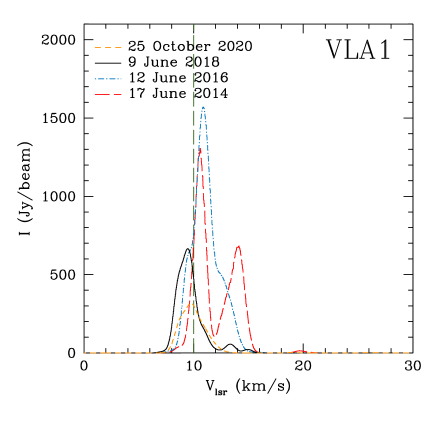
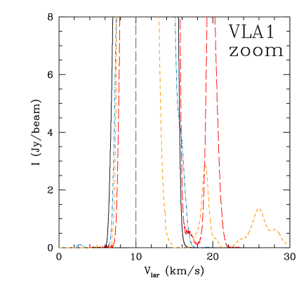
Figure 3: Comparison of the total sum of the H₂O maser spectra detected toward VLA 1 with the EVN in epochs 2014.46, 2016.45, 2018.44, and 2020.82. The vertical dashed dark-green line indicates the assumed systemic velocity of the region ($V_{\rm{lsr}}=+10.0$ km s^-1, Shepherd et al. 2003).

The number of 22 GHz H₂O maser features detected around VLA 1 has decreased from the EVN epoch 2014.46 to the EVN epoch 2020.82 (see Table 3). If we plot all the H₂O maser features detected in all the four EVN epochs, after correcting their positions as reported above, we see that these are always distributed along the radio continuum emission of VLA 1 presented by Rodríguez-Kamenetzky et al. (2020). This continuum emission was obtained at a resolution of tens of milliarcseconds by observing with the VLA a wide range of frequencies ($4-48$ GHz) in 2014. Rodríguez-Kamenetzky et al. (2020) concluded that VLA 1 is at the early stage of photoionization and it is driving a thermal radio jet at scale of about 0.1 arcsec ($\approx 130$ au). In Fig. 2 we overplot the H₂O maser features detected in the four EVN epochs to the continuum emission measured at Q-band by Rodríguez-Kamenetzky et al. (2020). The velocities of all the H₂O maser features are not showed in this figure, however, they are shown in the left panels of Fig. 13, where every EVN epoch is reported in a different panel. In order to better visualize the accordance of the maser features distribution with the position angle of the thermal radio jet, we make a linear fit of the maser features in each epoch. The results of these fits are shown in the right panel of Fig. 2 and their parameters are reported in Table 6. For the linear fit of epoch 2014.46, we do not consider the group of five maser features located south because their positions would strongly affect the position angle of the fitting line. This is not the case for the northeast and southeast maser features of epochs 2016.45 and 2018.44, respectively, which we indeed include in our linear fits. We see that the position angle of the fitted lines (see Fig. 2 and Table 6 for comparison) are consistent with the position angle of the thermal radio jet (solid gray line in Fig. 2, PA=+42^∘$\pm$5^∘; Rodríguez-Kamenetzky et al. 2020).

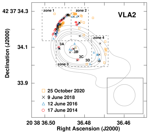
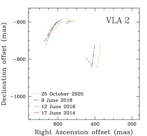
Figure 4: Comparison of the H₂O maser features detected toward VLA 2 (left panel) in the four EVN epochs (2014.46, 2016.45, 2018.44, and 2020.82) and superimposed to the natural-weighted continuum map at K-band (central frequency 22 GHz) of the thermal, collimated ionized wind emitted by VLA 2 obtained with the VLA by Carrasco-González et al. (2015). The light gray contours are 5, 10, 15, 20, 25, 50, and 75 times $\sigma=10\leavevmode\nobreak\ \rm{\mu Jybeam^{-1}}$ and the VLA beam is shown on the bottom right corner. The positions of the maser features are corrected assuming the proper motion of the subregion W75N(B) equal to the median proper motion measured for the 6.7 GHz CH₃OH maser features by Rygl et al. (2012), $\langle\mu_{\rm{\alpha}}\rangle=(-1.97\pm 0.10)\leavevmode\nobreak\ \rm{mas\leavevmode\nobreak\ yr^{-1}}$ and $\langle\mu_{\rm\delta}\rangle=(-4.16\pm 0.15)\leavevmode\nobreak\ \rm{mas\leavevmode\nobreak\ yr^{-1}}$. The size of the symbols are ten times the uncertainties of the absolute positions of the maser features (see Table 2). For clarity we show in the right panel the parabolic fit of the maser features of zone 1 and the linear fit of the maser features of zone 2 (north features) and zone 4 for each epoch. The reference position is $\alpha_{2000}=20^{\rm{h}}38^{\rm{m}}36^{\rm{s}}\!.43399$ and $\delta_{2000}=+42^{\circ}37^{\prime}34^{\prime\prime}\!\!.8710$. The parameters of the linear and parabolic fits are reported in Tables 6 and 7, respectively.

We note that the mean velocities along the line of sight of the maser features ($\langle V\rangle$, Col. 7 of Table 6) in the first three epochs, which are all around +11.5 km s^-1, and their similar maximum line of sight velocities ($V_{\rm{max}}\approx+16$ km s^-1, Col. 8 of Table 6) are largely different than those of epoch 2020.82 ($\langle V\rangle=+18.5$ km s^-1 and $V_{\rm{max}}=+26.3$ km s^-1). These differences might be explained either with an acceleration of the motion of VLA 1 along the line of sight and away from us, or with the variation of the masing conditions. Even though a combination of the two seems to be the case (see Fig. 3). In addition, we also note that the maser velocities are spatially mixed on the plane of the sky in each epoch.

3.1.2 VLA 2

The number of 22 GHz H₂O maser features detected around VLA 2 in the four EVN epochs ranges between 37 and 44 (see Table 3), which is roughly half of the number of maser features detected in the two previous VLBA epochs (88 and 68 in 2005.89 and 2012.54, respectively; S+14). These differences might not be because of the sensitivity of the EVN observations, which was better than that of the VLBA epochs (see Table 1 and ; ), but of the maser activity of the region. The maser distribution in the four EVN epochs is consistent with the elliptical shell observed for the first time by Kim et al. (2013) and confirmed by S+14. S+14 also measured a mean expansion velocity of the maser shell on the plane of the sky, which begun to expand in 1999 when the shell was quasi-circular and continued by becoming elliptical in 2007 (Torrelles et al. 2003; S+11a; Kim et al. 2013), of 4.9 $\rm{mas\,yr^{-1}}$ (30 km s^-1 at a distance of 1.3 kpc). However, the previous observations could not be properly compared because only those presented in Kim et al. (2013) were made in phase-reference mode and therefore the absolute positions of most of the maser features in the other epochs were unknown. For estimating the expansion velocity, S+14 assumed that the center of the shells coincides in the different epochs and consequently the measured expansion is radial. Since we were able to measure the absolute positions of the maser features in the four EVN epochs, we are now able to properly measure the expansion velocity. Nevertheless, we can compare our expansion velocities only in magnitude and not in direction with that measured by S+14. We plot all the H₂O maser features detected with the EVN

Table 5: Polynomial fit parameters of the H₂O maser features of zones 1 of VLA 2.

(1)	(2)	(3)	(4)	(5)	(6)
Epoch	$a$	$b$	$c$	$R^{2}$	Proper Motion
					($\rm{mas\leavevmode\nobreak\ yr^{-1}}$)	(km s-1)
2014.46	$-0.00757$	$8.08$	$-2714$	$0.85$	$-$	$-$
2016.45	$-0.0204$	$23.9$	$-7595$	$0.89$	$-$	$-$
2018.44	$-0.0118$	$13.3$	$-4332$	$0.96$	$-$	$-$
2020.82	$-0.00669$	$6.93$	$-2365$	$0.94$	$-$	$-$
					$-2.5$	$-15.4$

and overplotted to the continuum emission at K-band (Carrasco-González et al. 2015) in the left panel of Fig. 4. Here, we group the maser features in four different zones. As for VLA 1, the velocities of all the H₂O maser features detected in VLA 2 are showed in the right panels of Fig. 13.

Zone 1. This is located northeast. Interestingly, while S+14 found expanding motions, our data now shows the opposite trend, with apparent motions toward the central source. Indeed, the maser features seem to not trace an expansion, but they actually seem to ”bounce”. The maser features of epoch 2014.46 are generally slightly at northeast of those of epochs 2016.45 and 2018.44, which are more northeast than those of epoch 2020.82. This apparent ”bouncing” could be interpreted as evidence that the outflowing gas, where the masers arise, encounters an obstacle, as already proposed by Kim & Kim (2018). This obstacle can be either a much denser medium that stops the expansion of the gas (case A) or the absence of physical conditions, such as density and temperature, for producing the H₂O maser emission (case B). In case A, the impact of the gas with a denser medium might have produced an additional slow inward shock that pumped the maser features in the four EVN epochs. To estimate the proper motion of the gas on the plane of the sky due to this inward shock we fit the maser features of zone 1 with polynomials of second order, one per EVN epoch, and the results are shown in the right panel of Fig. 4 and the parameters are listed in Table 7. In addition in Fig. 5 we show the areas where the maser features considered in the polynomial fit are located. We note that only the areas of epochs 2014.46 and 2020.82 do not overlap and therefore their polynomial fits can be used to estimate the proper motion.

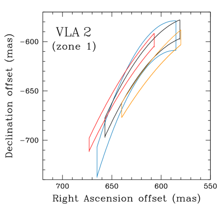
Figure 5: Each area represents the area in each epoch where the maser features considered in the polynomial fit (see Fig. 4 and Table 7) are located. The colors correspond to those used in Fig. 4.

Hence, we estimate the proper motion by measuring a mean distance between the curves of epochs 2014.46 and 2020.82 and the resulting velocity is equal to -2.5 $\rm{mas\,yr^{-1}}$ that corresponds to $\sim-15.4$ km s^-1 at a distance of 1.3 kpc, the minus sign indicates that the motion is opposite to the expansion measured by S+14. Although case A can be plausible, we should note that the curvature of the maser distribution in zone 1 is opposite than one would expect (see right panel of Fig. 4). In case B, the physical conditions of the gas in the northeast are not suitable for the maser emission and what we observe are maser features pumped by different outward shocks in each epoch. However, both cases are questioned by the presence of the broad maser feature VLA2.4.39 ($I=1.94$ Jy beam^-1, $\Delta v_{\rm{L}}=1.65$ km s^-1; see Table 17) that is located farther northeast of all the other maser features of zone 1. This maser feature shows physical parameters, such as the velocity ($V_{\rm{lsr}}=+16.35$ km s^-1), consistent with those of the other maser features of the zone. However, the presence of this isolated maser feature can also be justified by the presence of a belt of gas, between VLA2.4.39 and the other maser features, where the maser conditions are not met. Therefore, if the shock that pumped VLA2.4.39 is the same that pumped the maser features in the EVN epoch 2014.46, we can estimate the proper motion due to this shock. VLA2.4.39 is at about 53 mas from the front of the maser features detected in epoch 2014.46, therefore the proper motion is $7.9$ $\rm{mas\,yr^{-1}}$ that corresponds to $\sim 49$ km s^-1 at a distance of 1.3 kpc. This is higher than the expansion velocity measured by S+14 and the proper motions measured by Kim et al. (2013), $\sim 20-30$ km s^-1.

Table 6: Individual H₂O maser features around VLA 2 for which the velocity of the pumping shock is measured.

(1)	(2)	(3)	(4)	(5)
Epoch	maser	$V_{\rm{lsr}}$	Peak	Proper motion
	feature		Intensity (I)
		(km s-1)	(Jy beam-1)	($\rm{mas\,yr^{-1}}$)	(km s-1)
VLA 2 - zone 2 - below linear fit
2014.46	VLA2.1.04	$+4.26$	$5.78\pm 0.02$	$-$	$-$
2016.45	VLA2.2.07	$+5.63$	$0.67\pm 0.02$	$4.8$	$29.6$
2018.44	VLA2.3.06	$+6.27$	$5.86\pm 0.03$	$4.5$	$27.8$
2020.82	VLA2.4.13	$+0.65$	$0.38\pm 0.05$	$4.7$	$29.0$
				$4.6$	$28.4$
VLA 2 - zone 3 - group 3A
2014.46	VLA2.1.22	$+5.61$	$2.77\pm 0.01$	$-$	$-$
2016.45	VLA2.2.18	$+5.87$	$1.58\pm 0.02$	$2.0$	$12.3$
2018.44	VLA2.3.32	$+5.90$	$0.90\pm 0.02$	$2.0$	$12.3$
				$2.0$	$12.3$
VLA 2 - zone 3 - group 3B
2014.46	VLA2.1.09	$+21.19$	$0.27\pm 0.01$	$-$	$-$
2016.45	VLA2.2.12	$+13.45$	$10.42\pm 0.52$	$5.0$	$30.8$
2018.44	VLA2.3.13	$+12.80$	$9.10\pm 0.10$	$7.5$	$46.2$
				$6.2$	$38.3$
VLA 2 - zone 3 - group 3C
2014.46	VLA2.1.03	$+14.90$	$20.80\pm 0.25$	$-$	$-$
2018.44	VLA2.3.09	$+14.69$	$4.77\pm 0.13$	$1.3$	$8.0$

In 2015, Carrasco-González et al. presented the most recent continuum maps of VLA 2, which were obtained by observing four different frequency bands (C, U, K, and Q) with the VLA in 2014. From these new maps it was possible to verify the variation of collimation of the outflow emitted from VLA 2 as traced by the H₂O maser features from 1999 to 2012 (S+14). We can therefore compare our maser distributions with the VLA continuum emission at K-band (see Fig. 4). The asymmetric morphology of the K-band continuum emission, which shows a weaker emission toward southwest and none toward northeast, suggests the presence of an obstacle toward northeast as we supposed above. This obstacle might be an inhomogeneity within the dusty disk or envelope supposed by Carrasco-González et al. (2015). In particular, the distribution of the maser features of zone 1 seems to be the continuation toward northwest of the last external contour of the continuum emission at 50 $\mu$Jy beam^-1(see Fig. 4), even though no continuum emission is detected where these maser features arise.
We note that the velocity range of the maser features of zone 1 in the four EVN epochs ($-11$ km s^-1$<V_{\rm{lsr}}^{\rm{2014.46}}<+17$ km s^-1, $-16$ km s^-1$<V_{\rm{lsr}}^{\rm{2016.45}}<+17$ km s^-1, $-16$ km s^-1$<V_{\rm{lsr}}^{\rm{2018.44}}<+16$ km s^-1, and $+6$ km s^-1$<V_{\rm{lsr}}^{\rm{2020.82}}<+17$ km s^-1) is similar to that covered in the VLBA epoch 2012.54 ($-10$ km s^-1$<V_{\rm{lsr}}^{\rm{2012.54}}<+18$ km s^-1; S+14), even though the range observed in the EVN epoch 2020.82 shows only redshifted velocities. This might suggest that the maser features of zone 1 traced the same shock, that moved outward, from 2012.54 to 2018.44, and then they quenched any time between 2018.44 to 2020.82. We also note that, in the first three EVN epochs, the blue- and redshifted maser features do not follow any particular spatial distribution, that is blue- and redshifted maser features are spatially coincident and do not show any velocity gradient. This might further indicate that the gas expands along the walls of the denser medium when encountering it. Consequently, the maser features in the last EVN epoch (2020.82) might trace a different shock that still move outward rather than inward, according to the morphology of the maser distribution. This might exclude the possible inward shock supposed above when we discussed case A.

Zone 2. The low number of H₂O maser features of zone 2 (northwest, see Fig. 4) detected from the VLBA epoch 2012.54 to the EVN epoch 2018.44 and their total H₂O maser intensity (see Sect. 3.2.2) indicate a low maser activity in this zone since the appearance of the elliptical maser distribution. However, the maser features detected in the last EVN epoch 2020.82 are in number about three times more and their total H₂O maser intensity is almost ten times higher than previously detected (see Sect. 3.2.2), suggesting a sudden increment of the maser activity as never observed before in the northeast part of the maser distribution, neither when the distribution was quasi-circular (Torrelles et al. 1997, 2003; S+11a) nor afterward (Kim et al. 2013; ; ). Comparing only the EVN epochs, we note that all the maser features in zone 2 north of declination 42^∘37’34.​​”2 in Fig. 4 have a velocity range between $-1$ km s^-1 and +9 km s^-1, that is, they are all blueshifted, with the exception of VLA2.4.12 that shows a redshifted velocity of $V_{\rm{lsr}}=+12.77$ km s^-1. The rest of the maser features of zone 2 (south of declination 42^∘37’34.​​”2 in Fig. 4), which are the only ones detected on the continuum emission at K-band (see Fig. 4), show much higher redshifted velocities (+15 km s^-1$<V_{\rm{lsr}}<+23$ km s^-1). Differently from zone 1, we see that the maser features in zone 2 detected in one epoch are always detected outward with respect the previous epoch. To better estimate the apparent motion between different epochs, we make a linear fit of the maser features in each epoch. In particular, we are able to measure the expansion velocity of the north maser features in zone 2 by considering the distance of the median point of the line of one epoch from the line of the next epoch. The results are reported in Table 6 and in the right panel of Fig. 4. The expansion velocities on the plane of the sky measured between the epochs 2016.45 and 2018.44 (3.8 $\rm{mas\,yr^{-1}}$) and between epochs 2018.44 and 2020.82 (4.3 $\rm{mas\,yr^{-1}}$) are consistent with the expansion velocity of 30 km s^-1 (4.9 $\rm{mas\,yr^{-1}}$) measured by S+14. In zone 2 it is also possible to identify four maser features, each detected in a different EVN epoch, located below the linear fits and at the center of the dashed rectangle that highlights zone 2 in Fig. 4, that apparently seem to trace an outward motion. These maser features are VLA2.1.04, VLA2.2.07, VLA2.3.06, and VLA2.4.13 (see Table 8). Although these maser features have different line of sight velocities (see Col.3 of Table 8), we can estimate the expansion velocity between the four EVN epochs by assuming that the shock that pumped them is the same. We find a proper motion of 4.8 $\rm{mas\,yr^{-1}}$ ($\sim 30$ km s^-1 at 1.3 kpc) between the epochs 2014.46 and 2016.45, 4.5 $\rm{mas\,yr^{-1}}$ ($\sim 28$ km s^-1) between epochs 2016.45 and 2018.44, and 4.7 $\rm{mas\,yr^{-1}}$ ($\sim 29$ km s^-1) between the epochs 2018.44 and 2020.82 (see Table 8). The mean proper motion between epochs 2014.46 and 2020.82 is equal to 4.6 $\rm{mas\,yr^{-1}}$ ($\sim 28$ km s^-1) that is again consistent with the expansion velocity measured by S+14 on the plane of the sky, that is 30 km s^-1. The consistency of the expansion velocities measured from the maser features of zone 2 with that measured previously by S+14 is a further clue of the presence, since epoch 2014.46, of an obstacle in front of the expanding gas in zone 1 that is absent in front of the gas in zone 2 that can freely expand.

Zone 3. The H₂O maser features of zone 3 are all located toward the bright core of the continuum emission observed by Carrasco-González et al. (2015, see Fig. 4) and show velocities in the range between +1 km s^-1 and +22 km s^-1. We note that the blueshifted maser features are always located outward than the redshifted in all the epochs. Looking at Fig. 4 we can divide the maser features in zone 3 in four groups: one in the east (group 3A), one in the center (group 3B), one in the south (group 3C), and the fourth in the southwest (group 3D). Group 3B coincides with the peak of the continuum emission at K-band ($\sim 800$ $\mu$Jy beam^-1), groups 3A and 3C are located between the contours at 25$\sigma$ (250 $\mu$Jy beam^-1) and 50$\sigma$ (500 $\mu$Jy beam^-1) of Fig. 4, while group 3D between the contours at 20$\sigma$ (200 $\mu$Jy beam^-1) and 25$\sigma$ (250 $\mu$Jy beam^-1). For the first three groups (3A-3C), we can identify maser features with similar velocity in at least two epochs and we are therefore able to estimate their proper motions. In particular, we identify in group 3A a maser feature in three consecutive epochs (from 2014.46 to 2018.44) corresponding to VLA2.1.22, VLA2.2.18, and VLA2.3.32 (see Table 8). We measured a constant velocity of $\sim$12 km s^-1 (2.0 $\rm{mas\,yr^{-1}}$) pointing slightly toward southwest between epochs 2014.46 and 2016.45 and between epochs 2016.45 and 2018.44 (see Table 8). The maser features VLA2.1.03 and VLA2.3.09 of group 3C can be considered tracing the same gas and therefore the estimated proper motion is $\sim$8 km s^-1 (1.3 $\rm{mas\,yr^{-1}}$; see Table 8). Both proper motions of groups 3A and 3C are much lower than that measured by S+14. The identification of common maser features with similar $V_{\rm{lsr}}$ in group 3B is very difficult. However, we can identify three maser features by considering their relative position in Fig 4. These are VLA2.1.09, VLA2.2.12, and VLA2.3.13 (see Table 8). The proper motion is then $\sim$31 km s^-1 (5.0 $\rm{mas\,yr^{-1}}$) between epochs 2014.46 and 2016.45, and $\sim$46 km s^-1 (7.5 $\rm{mas\,yr^{-1}}$) between epochs 2016.45 and 2018.44 (see Table 8). The mean proper motion between epochs 2014.46 and 2018.44 is about 38 km s^-1 (6.2 $\rm{mas\,yr^{-1}}$) that is slightly higher than the expansion velocity of 30 km s^-1 measured by S+14.

Zone 4. This zone is located southwest and the H₂O maser features distribution is roughly aligned north-south as observed previously (Torrelles et al. 2003; Kim et al. 2013;S+14). No H₂O maser emission was detected toward this zone in the EVN epoch 2014.46. A comparison with the continuum emission at K-band reported by Carrasco-González et al. (2015) reveals that the maser features of zone 4, which are all redshifted (+16 km s^-1$<V_{\rm{lsr}}<+29$ km s^-1), are all associated with the weak continuum emission at around 200-300 $\mu$Jy beam^-1 (see Fig. 4). The results of the linear fit of the maser features are reported in Table 6 and displayed in the right panel of Fig. 4. Because the linear fit of epoch 2016.45 crosses that of epoch 2018.44 (see right panel of Fig. 4), we can estimate an expansion velocity on the plane of the sky only between epochs 2018.44 and 2020.82. This is the largest ever measured toward the maser features around VLA 2 and its value is equal to 12.7 $\rm{mas\,yr^{-1}}$ ($\sim$78 km s^-1). This high velocity might suggest that the gas does not encounter any dense matter toward southwest that could slow it down.

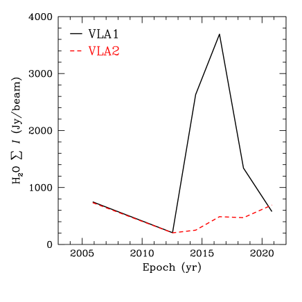
Figure 6: Comparison of the total sum of the H₂O maser intensity ($I$) measured toward VLA 1 and VLA 2 with the VLBI in epochs 2005.89 (VLBA, S+11a, ), 2012.54 (VLBA, S+14, ), 2014.46 (EVN), 2016.45 (EVN), 2018.44 (EVN), and 2020.82 (EVN). The lowest intensities coincide with the minimum of activity registered toward W75N(B) by the 22-m Pushchino telescope in May-July 2012 (Krasnov et al. 2015).

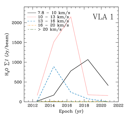
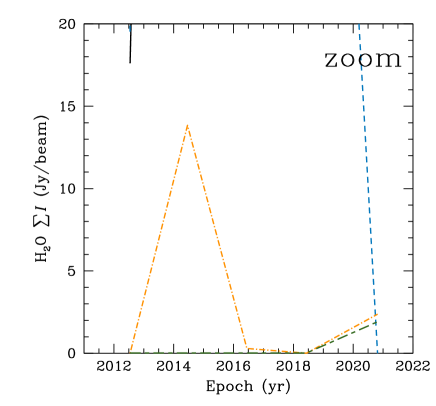
Figure 7: Comparison of the total sum of the H₂O maser intensity ($I$) for five different ranges of velocities in VLA 1 as measured in epochs 2012.54 (VLBA, S+14, ), 2014.46 (EVN), 2016.45 (EVN), 2018.44 (EVN), and 2020.82 (EVN).

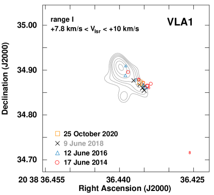
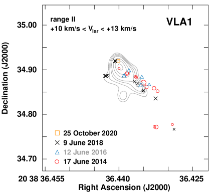
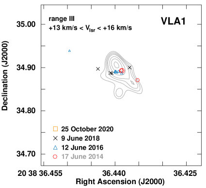
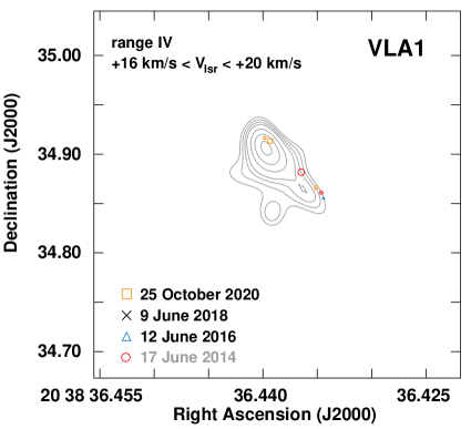
Figure 8: Comparison of the H₂O maser features detected for five different ranges of velocities in VLA 1 in the four EVN epochs 2014.46, 2016.45, 2018.44, and 2020.82. The size of the symbols are scaled logarithmically according to their peak intensities. The epoch for which the maximum of the intensities is registered for each velocities range is colored in light gray. The assumed velocity of the region is $V_{\rm{lsr}}=+10.0$ km s^-1 (Shepherd et al. 2003).

3.2 Intensity variability

3.2.1 VLA 1

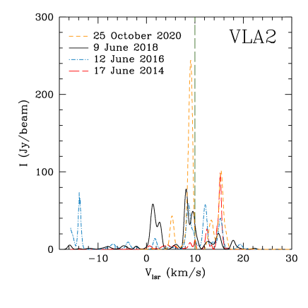
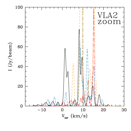
Figure 9: Comparison of the total sum of the H₂O maser spectra detected toward VLA 2 with the EVN in epochs 2014.46, 2016.45, 2018.44, and 2020.82. The vertical dashed dark-green line indicates the assumed systemic velocity of the region ($V_{\rm{lsr}}=+10.0$ km s^-1, Shepherd et al. 2003).

The total H₂O maser intensity ($\sum{I}$) of the maser features first had an increment between the VLBA epoch 2012.54 (S+14) and the EVN epoch 2016.45 and then it decreased again till the last EVN epoch 2020.82. This variation of the intensity can be seen in Fig. 6, where we also show the intensities measured in epochs 2005.89 and 2012.54 with the VLBA (; ). The lowest intensity was measured in 2012.54 ($\sum I=206.31$ Jy beam^-1) by S+14 and it coincides with the minimum of activity registered toward W75N(B) by the 22-m Pushchino telescope in May-July 2012 (Krasnov et al. 2015). The H₂O maser features cover a large line of sight velocity range from +7.8 km s^-1 to +26.4 km s^-1 over the four EVN epochs and, as mentioned before, with maser features with line of sight velocities $\geq+20$ km s^-1 detected only in epoch 2020.82 (see Table 3 and Fig. 3). We therefore compare the intensities for five different ranges of velocities along the line of sight (ranges I-V) in Fig. 7 and we plot the corresponding maser features superimposed to the continuum emission at Q-band (Rodríguez-Kamenetzky et al. 2020) in the five panels of Fig. 8. We note that each range of velocities has the maximum of total intensity at different epochs (the corresponding epoch is colored in light gray in Fig. 8). In particular the maximum is reached earlier for the ranges with the highest velocities, except for the maser features with velocities $\geq+20$ km s^-1 (range V) that are detected only in epoch 2020.82. Indeed, we see that $\sum{I}$ of the maser features with +7.8 km s^-1$<V_{\rm{lsr}}<+10$ km s^-1(range I), which are the only blueshifted features with respect to the systemic velocity of the region ($V_{\rm{lsr}}=+10.0$ km s^-1; Shepherd et al. 2003), and with +10 km s^-1$<V_{\rm{lsr}}<+13$ km s^-1 (range II) show the maximum in epochs 2018.44 and 2016.45, respectively. Whereas the ranges +13 km s^-1$<V_{\rm{lsr}}<+16$ km s^-1 (range III) and +16 km s^-1$<V_{\rm{lsr}}<+20$ km s^-1 (range IV) show their maximum in epoch 2014.46. Furthermore, we note that the maser features of ranges I, II, which are respectively within $\mp$3 km s^-1 from the systemic velocity, and IV are mainly located along the southwestern tail of the thermal radio jet at Q-band, and in particular the intensity of ranges I and II reaches its maximum when the maser features are along this tail (see Fig. 8). A few maser features of ranges II and IV are close to the position of the strong core of the continuum emission at Q-band and these all but one are detected in the last two epochs, the one is detected in epoch 2014.46 (range II). Most of the maser features of range III are instead aligned east-west below the core of the continuum emission at Q-band and its intensity reaches the maximum in epoch 2014.46. The most redshifted maser features (range V) are the weakest ones among all of those detected in the VLBA and EVN epochs, this can be due to the fact that they have arisen only recently. These maser features are located in the very west edge of the southern tail and slightly north of the core. The spatial coincidence of the blue- and redshifted maser features of ranges I and II may suggest that the maser features are tracing the central part of one of the lobes of the thermal jet, and that this has such an inclination that the maser features located on the surface closer to us appear slightly blueshifted, while those located on the opposite surface appear slightly redshifted.

3.2.2 VLA 2

The total intensity of the H₂O maser emission almost constantly increased between the VLBA epoch 2012.54 and the EVN epoch 2020.82 (see Fig. 6). This reflects the fact that the maser features in the four EVN epochs, although half in number, are actually brighter than those detected in the two previous VLBA epochs (see Table 3 and ; ). We show the total sum of the H₂O maser spectra detected towards VLA 2 in the four EVN epochs in Fig. 9, from where the complexity of the H₂O maser emission around VLA 2 is further confirmed.
We compare the $\sum{I}$ for the four zones (see Sect. 3.2.2) in Fig. 10. Here we see that zone 1 in the four EVN epochs shows increments of intensity between epochs 2014.46 and 2016.45, and between epochs 2018.44 and 2020.82, with a slight decrement between epochs 2016.45 and 2018.44. The increments of total intensity are due to the high intensity of individual maser features rather than to their number (see Tables 11, 13, 15, and 17), indicating that the masing conditions are more favorable inward than outward. Also the maser features of zone 2 show an increment of $\sum{I}$ between epochs 2018.44 and 2020.82 similar to that of zone 1 between the same two epochs, this is 127 Jy beam^-1 for zone 1 and 137 Jy beam^-1 for zone 2.

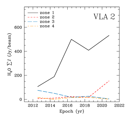
Figure 10: Comparison of the total H₂O maser intensity in the four zones of VLA 2 (see Fig.4) measured in epochs 2012.54 (VLBA, S+14, ), 2014.46 (EVN), 2016.45 (EVN), 2018.44 (EVN), and 2020.82 (EVN).

In zone 3, we instead observe a decrement of $\sum{I}$ between the VLBA epoch 2012.54 and the four EVN epochs. We detected the brightest maser features in the EVN epoch 2014.46 toward south (VLA2.1.01 and VLA2.1.03, each with $\rm{I}\approx 21$ Jy beam^-1) while the rest of the maser features of zone 3 show a maser intensity $\rm{I}<13$ Jy beam^-1 in all four EVN epochs, with the brightest of them detected toward the center of the continuum emission. The trend of $\sum{I}$ in zone 4 between epochs 2016.45 and 2020.82 is identical to that observed for the maser features of zone 3.

3.3 Maser polarization

The analysis of the polarized emission from the H₂O maser features detected in the four EVN epochs allow us to compare, in addition to the magnetic field that we will present in Section 4, some physical parameters of the maser features and of the gas where they arise.

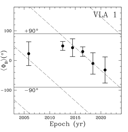
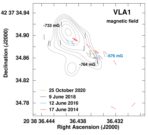
Figure 11: Multi-epoch comparison of $\langle\Phi_{\rm{B}}\rangle$ angles for VLA 1 (left panel). The epochs are 2005.89 (VLBA, S+11a, ), 2012.54 (VLBA, S+14, ), 2014.46 (EVN), 2016.45 (EVN), 2018.44 (EVN), and 2020.82 (EVN). The two horizontal solid black lines indicates the $\pm 90$^∘ angles. The dashed gray lines represents the best linear fit results of the data considering that the position angle of a magnetic field vector has contemporary multiple values equal to $\langle\Phi_{\rm{B}}\rangle=\langle\Phi_{\rm{B}}\rangle\pm 180$^∘. The slopes of these lines are $m_{\rm{VLA\,1}}=(-15^{\circ}\!.38\pm 1^{\circ}\!.80)\leavevmode\nobreak\ \rm{yr^{-1}}$. Right panel: Magnetic field vectors and strength along the line of sight (next to the corresponding maser feature) as estimated from all the linearly and circularly polarized maser features detected around VLA 1 during the four EVN epochs (2014.46, 2016.45, 2018.44, and 2020.82). The vectors are superimposed to the uniform-weighted continuum map at Q-band (central frequency 44 GHz) of the thermal jet driven by VLA 1 (Rodríguez-Kamenetzky et al. 2020). For more details see caption of Fig. 2.

3.3.1 VLA 1

We note that the highest values of $P_{\rm{l}}$ were measured in epochs 2014.46 (15.6%) and 2018.44 (10.6%) and the corresponding maser features are located far southwest of the continuum emission at Q-band (2014.46) and at west of the bright core of this continuum emission (2018.44). Whereas the lowest values of $P_{\rm{l}}$ are all measured in epoch 2020.82 (see Table 3).
As described in Sect. 2, we can estimate some intrinsic characteristics of the maser features by modeling the linearly polarized emission with the FRTM code. The averaged intrinsic linewidth is larger in epoch 2014.46 ($\langle\Delta V_{\rm{i}}\rangle$$=3.0^{+0.2}_{-0.3}$ km s^-1) and then consistently decreases, to reach a minimum value of $2.6^{+0.1}_{-0.3}$ km s^-1 in epoch 2020.82. This implies that the gas temperature of the region $T$ has also decreased from epoch 2014.46 to epoch 2020.82. Indeed, from the equation $T\approx 100\cdot(\langle\Delta V_{\rm{i}}\rangle/0.5)^{2}$ (Nedoluha & Watson 1992), that is valid if the broadening of the maser line due to the turbulence is negligible, we have that $T_{\rm{2014.46}}=3600^{+496}_{-684}$ K and $T_{\rm{2020.82}}=2704^{+212}_{-588}$ K. If the H₂O masers are pumped by nondisocciative shocks the gas can reach temperatures around 4000 K and above this threshold the H₂O molecule is dissociated (Kaufman & Neufeld 1996). However, the estimated high temperatures indicate that the contribution of the turbulence to $\Delta V_{\rm{i}}$ is not actually negligible. However, if we assume that this contribution is constant in time and everywhere in the source we can still qualitatively compare the estimated temperatures between the different epochs. The averaged emerging brightness temperature ($\langle T_{\rm{b}}\Delta\Omega\rangle$) instead increases from epoch 2014.46 to epoch 2020.82 (see Table 3), this might indicate that the saturation level of the maser features increases from one epoch to the other. This is related to the efficiency of the pumping mechanism. Indeed the saturation regime is reached when the stimulated emission rate becomes larger than the decay rate to the upper level of the maser transition, in other words the pumping mechanism is not able anymore to provide enough population inversion between the maser levels. In the case of the H₂O maser the pumping mechanism is due to the shocks produced by the outflow hitting the surrounding matter. Therefore, the shocks should have lost part of their energy from one epoch to the other, which might also be suggested by the estimated gas temperature.
Circular polarization was measured only in epochs 2016.45 and 2018.44 (see Appendix A) when the total H₂O maser intensity reached its highest values. From the three circularly polarized maser features, we measure a magnetic field strength along the line of sight between $-676\pm 102$ mG (epoch 2016.45; see Table 12) and $-764\pm 22$ mG (epoch 2018.44; see Table 14), which are consistent with what S+11a and S+14 measured in the previous two VLBA epochs ($-400\leavevmode\nobreak\ \rm{mG}<B_{\rm{||}}^{\rm{2005.89}}<+810$ mG and $-540\leavevmode\nobreak\ \rm{mG}<B_{\rm{||}}^{\rm{2012.54}}<+18$ mG). We note that the positive and negative signs of $B_{\rm{||}}$ indicate that the magnetic field is pointing away and toward the observer, respectively.

3.3.2 VLA 2

We note that all the linearly polarized maser features in the four EVN epochs, but VLA2.1.24 ($P_{\rm{l}}=4.6\leavevmode\nobreak\ \%$), show a $P_{\rm{l}}$ in the range between 0.2% and 2.7% (see Table 3). The outputs of the FRTM code provides consistent $T_{\rm{b}}\Delta\Omega$ values in all EVN epochs, only four and one maser features show $T_{\rm{b}}\Delta\Omega$ on the order of $10^{6}$ and $10^{10}$ K sr respectively, and consistent $\Delta V_{\rm{i}}$ in three of the four EVN epochs. In epoch 2014.46 we have $\Delta V_{\rm{i}}$$<2$ km s^-1 while in the other three EVN epochs $\Delta V_{\rm{i}}$$>2$ km s^-1 with a few exceptions (VLA2.2.22, VLA2.3.21, and VLA2.3.23). As we already made previously for VLA 1 (Sect. 3.3.1), and keeping in mind that the values do not actually indicate the actual temperature of the gas, we can estimate the mean temperature from the $\Delta V_{\rm{i}}$ values and we then have $T_{\rm{2014.46}}=1024^{+272}_{-240}$ K, $T_{\rm{2016.45}}=3364^{+480}_{-448}$ K, $T_{\rm{2018.44}}=1764^{+1600}_{-608}$ K, and $T_{\rm{2020.82}}=3364^{+236}_{-864}$ K. We note that all the linearly polarized maser features in epoch 2014.46 are located northeast, where the expanding gas is supposed to encounter a denser medium.
We were also able to measure $B_{\rm{||}}$ from the circularly polarized maser emission of a total of five maser features in the three EVN epochs 2016.45 ($-1498\pm 225$ mG and $-2426\pm 364$ mG, Table 13), 2018.44 ($-355\pm 69$ mG and $+439\pm 66$ mG, Table 15), and 2020.82 ($-452\pm 68$ mG, Table 17), all of them are located north - northeast. These values are larger than those measured in epochs 2005.89 ($-186\leavevmode\nobreak\ \rm{mG}<B_{\rm{||}}^{\rm{2005.89}}<+957$ mG; S+11a) and 2012.54 ($-152\leavevmode\nobreak\ \rm{mG}<B_{\rm{||}}^{\rm{2005.89}}<-103$ mG; S+14) with the VLBA.

4 Magnetic Field

We discuss the magnetic field around VLA 1 and VLA 2 in Sects. 4.1 and  4.2, respectively. Here, we are able to estimate and compare the orientation of the magnetic field from the linear polarization vectors measured in the four EVN epochs. We determine for each epoch the error-weighted orientation of the magnetic field ($\langle\Phi_{\rm{B}}\rangle$), which are listed in Table 3. We note that the position angle of a magnetic field vector on the plane of the sky has three values contemporary: $\Phi_{\rm{B}}$ and $\Phi_{\rm{B}}\pm 180$^∘. Therefore, we can state that the magnetic field vectors have a sort of periodicity of 180^∘ that exists only as a consequence of how $\Phi_{\rm{B}}$ is defined on the plane of the sky: positive if measured counterclockwise from north and negative if measured clockwise from north.

4.1 VLA 1

We plot $\langle\Phi_{\rm{B}}\rangle$ as function of time in the left panel of Fig. 11, as measured in the two previous VLBA epochs (2005.89 and 2012.54) and in the four EVN epochs. Here, we also show a 180^∘-periodicity linear fit (dashed gray lines) that has a slope of $m_{\rm{VLA\,1}}=(-15^{\circ}\!.38\pm 1^{\circ}\!.80)\leavevmode\nobreak\ \rm{yr^{-1}}$. However, the apparent rotation is not due to calibration uncertainties (see Table 1) or to maser polarization variability, which can influence the relation between the magnetic field orientation and the polarization vectors only if the H₂O maser features are highly saturated (this is not our case), but it is simply the consequence of averaging the $\Phi_{\rm{B}}$ angles that are estimated from linear polarization vectors measured in different locations along VLA 1, where the magnetic field is actually differently oriented. Therefore, a punctual comparison between the magnetic field vectors measured in the different epochs is necessary. However, this cannot be done with common polarized maser features detected in consecutive epochs because of the maser variability on short timescales. Instead, what we can do is a comparison of all the magnetic field vectors estimated in all the epochs. Indeed, we plot each single magnetic field vector estimated from all the linearly polarized maser features detected in the four EVN epochs in the right panel of Fig. 11. Here, we can see that the magnetic field vectors estimated in similar location, but in different epochs, seem to represent a quasi-static magnetic field. We can therefore consider the magnetic field vectors estimated from the H₂O maser features in one epoch as representative of the magnetic field in those locations rather than in that time. Consequently, we can gather the magnetic field vectors of all the EVN epochs and consider them as measurements done at the same time. This allows us to compare the magnetic field with the continuum emission at Q-band (see Fig. 11). The magnetic field vectors seem to follow the morphology of the continuum emission, in particular the internal vectors are in accordance with the radio continuum contours (right panel of Fig. 11). This suggests that the magnetic field is along the thermal jet and it bends toward south at the southwest end of the thermal jet, and toward north at the northeast end. In addition, we note that the magnetic field orientation in the northeast and in the far southwest coincides with that of the large-scale magnetic field vectors reported by (Palau et al. 2021, their Fig.2) who showed the 1.3 mm polarized continuum emission of W75N(B) as observed by Alves et al. (in preparation).

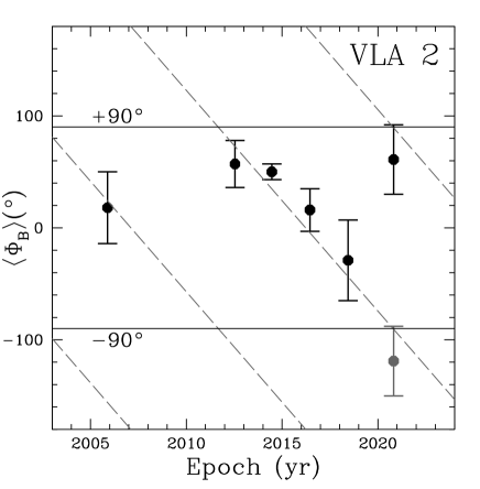
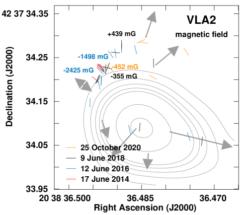
Figure 12: Multi-epoch comparison of $\langle\Phi_{\rm{B}}\rangle$ angles for VLA 2 (left panel). The epochs are 2005.89 (VLBA, S+11a, ), 2012.54 (VLBA, S+14, ), 2014.46 (EVN), 2016.45 (EVN), 2018.44 (EVN), and 2020.82 (EVN). The gray point indicates the $\langle\Phi_{\rm{B}}\rangle$ angle measured in 2020.82 after a rotation of 180^∘, considering that $\langle\Phi_{\rm{B}}\rangle=\langle\Phi_{\rm{B}}\rangle\pm 180$^∘. The two horizontal solid black lines indicates the $\pm 90$^∘ angles. The dashed gray lines represents the best linear fit results of the data considering that the position angle of a magnetic field vector has contemporary multiple values equal to $\langle\Phi_{\rm{B}}\rangle=\langle\Phi_{\rm{B}}\rangle\pm 180$^∘. The slopes of these lines are $m_{\rm{VLA\,2}}=(-19^{\circ}\!.73\pm 1^{\circ}\!.89)\leavevmode\nobreak\ \rm{yr^{-1}}$. Right panel: Magnetic field vectors and strength along the line of sight (next to the corresponding maser feature) as estimated from the linearly and circularly polarized maser features detected around VLA 2 during the four EVN epochs (2014.46, 2016.45, 2018.44, and 2020.82) and superimposed to the natural-weighted continuum maps at K-band (central frequency 22 GHz) of the thermal, collimated ionized wind emitted by VLA 2 (Carrasco-González et al. 2015). For more details see caption of Fig. 4. The arrows represent the direction of the proper motions on the plane of the sky reported in Tables 6, 7, and 8, and the arrows length is proportional to their magnitudes. The double arrow in the northeast indicates the uncertainties of the motion direction, due to the presence of an inward motion (case A) or of an outward motion (case B) of the gas as explained in Sect. 3.1.2.

The three circularly polarized maser features are associated with the ends of the thermal jet as observed at Q-band (see Fig. 11) and the estimated magnetic field points toward us (see Sect. 3.3.1). The 3D magnetic field strength can be estimated from $|B|=\langle|B_{||}|\rangle/\rm{cos}\langle\theta\rangle$ (if $\theta\neq\pm 90$^∘), where $\langle|B_{||}|\rangle$ and $\langle\theta\rangle$ are the error-weighted mean values of $|B_{||}|$ and $\theta$, respectively. We must note that the magnetic field derived from the circularly polarized emission of the H₂O maser features can be very high because these masers probe shocked gas, so it is not representative of the whole region. We then have in the two EVN epochs $|B|^{\rm{2016.45}}>2.0$ G, which is a lower limit obtained by considering $\theta=71$^∘, and $\langle|B|^{\rm{2018.44}}\rangle=3.6$ G. Both these values are much larger than what was measured on average in the VLBA epochs ($\langle|B|^{\rm{2005.89}}\rangle\approx 0.7$ G and $\langle|B|^{\rm{2012.54}}\rangle>0.1$ G; ; ). The differences might be due to the increment of the magnetic field strength or to the hydrogen number density of the 22 GHz H₂O maser. In the latter case, by considering the relation $|B|\propto n_{\rm{H_{2}}}^{0.65}$ (Crutcher et al. 2010), we can estimate an increment of $n_{\rm{H_{2}}}^{\rm{H_{2}O}}$ of one order of magnitude between the VLBA epoch 2005.89 and the EVN epoch 2018.44.

4.2 VLA 2

Similarly to VLA 1, we observe an apparent clockwise rotation of $\langle\Phi_{\rm{B}}\rangle$ from the VLBA epoch 2015.89 to the EVN epoch 2020.82 (see left panel of Fig. 12). In this case we notice that $\langle\Phi_{\rm{B}}\rangle$ measured in the EVN epoch 2020.82 is on a different 180^∘-periodicity line with respect to those of the previous EVN epochs. The slope of the 180^∘-periodicity lines is $m_{\rm{VLA\,2}}=(-19^{\circ}\!.73\pm 1^{\circ}\!.89)\leavevmode\nobreak\ \rm{yr^{-1}}$, which might indicate that the rotation in VLA 2 is faster than in VLA 1. As explained in the case of VLA 1, the apparent rotation of $\langle\Phi_{\rm{B}}\rangle$ can be affected by the location of each maser feature for which we are able to estimate the magnetic field vectors and it cannot therefore be taken at face value. Indeed, despite our earlier claims (S+14), we now think there is no evidence for such a rotation. A comparison of the magnetic field vectors estimated in the four EVN epochs is reported on the right panel of Fig. 12. Two main aspects can be observed here, firstly almost all the magnetic field vectors are located northeast and secondly the magnetic field vectors estimated in one epoch can be considered representative of a quasi-static magnetic field in those locations rather than in that time. The magnetic field is generally, within the errors, perpendicular to the expansion velocities of the gas, which are represented with arrows in Fig. 12, all around VLA 2 and it is parallel only in the northeast where the expanding gas encounters the denser matter. The fact that the magnetic field vectors are along the shock front is not surprising. Indeed, H₂O masers arise behind fast C- or J-type shocks (e.g., Kaufman & Neufeld 1996; Hollenbach et al. 2013) that, while propagating in the ambient medium, alter the initial magnetic field configuration. As explained in details in Goddi et al. (2017), the magnetic field component perpendicular to the shock velocity is compressed and might dominate the parallel component, that remains unaffected, consequently the resulting magnetic field probed by the H₂O maser features might be expected to be along the shock front. The sudden change of the orientation of the magnetic field vectors in the northeast cannot be explained with the typical 90^∘-flip because the estimated $\theta$ angles of those H₂O maser features are much greater than 55^∘ (see Sect. 2). Therefore, this can be justified with a variation of the ratio between the perpendicular and the parallel components of the magnetic field with respect to the expanding velocity. In other words, even though the shock is still able to pump the H₂O molecules in order to produce the maser emission, it is not able anymore to compress enough the perpendicular component of the magnetic field in order to make it dominating over the parallel component. This can be considered a further clue in favor of the presence of a very dense gas in the northeast where the magnetic field is oriented northeast-southwest.

Table 7: Comparison of the hydrogen number densities of the gas in the northeast (zone 1) of VLA 2.

(1)	(2)	(3)	(4)	(5)
Epoch	Maser	$|B|$	$n_{\rm{H_{2}}}$	$n_{\rm{H_{2}}}$
	feature	(G)	equation	($\rm{cm^{-3}}$)
2005.89	VLA 2.16, VLA 2.17	3.4	$n_{1}$	$1.2\cdot 10^{9}$
	VLA 2.22, VLA 2.24
2012.54	VLA2.44	1.5	$n_{2}=0.3\cdot n_{1}$	$3.6\cdot 10^{8}$
2016.45	VLA2.2.27	27.8	$n_{3}=89\cdot n_{2}$	$3.2\cdot 10^{10}$
2018.44	VLA2.3.39	$0.6$	$n_{4}=0.003\cdot n_{3}$	$10^{8}$
2020.82	VLA2.4.27	$0.6$	$n_{5}=n_{4}$	$10^{8}$

We also compare the magnetic field vectors with the morphology of the continuum emission at K-band obtained by Carrasco-González et al. (2015) with the VLA in Fig. 12. Here, we see that some vectors seems to follow the morphology of the continuum emission suggesting a possible correlation between the magnetic field orientation and the shaping of the continuum emission. In addition, the orientation of the magnetic field vectors in the northeast of VLA 2 agree well to the values reported by Palau et al. (2021) at large scales ($\sim 1.3^{\prime\prime}$), using submillimeter continuum data, indicating that the magnetic field at small scales might connect with the magnetic field at large scales.
To properly compare the magnetic field strength measured in different epochs, we need to estimate $|B|$ (see Sect. 4.1). We have $|B_{\rm{VLA2.2.17}}|=9.5$ G and $|B_{\rm{VLA2.2.27}}|=27.8$ G in epoch 2016.45, $|B_{\rm{VLA2.3.14}}|>0.7$ G and $|B_{\rm{VLA2.3.39}}|>0.6$ G in epoch 2018.44 (we assume a lower value of $\theta=53$^∘, see Table 3), and $|B_{\rm{VLA2.4.27}}|=0.6$ G in epoch 2020.82. As we already mentioned in Sect.4.1, a variation of the magnetic field strength might largely be due to a variation of $n_{\rm{H_{2}}}$ of the gas where the H₂O maser features arise. This variation follows the empirical equation of Crutcher et al. (2010) that is reported in Sect. 4.1. Considering the measurements of $B$ made in the northeast of VLA 2 (zone 1), we can estimate $n_{\rm{H_{2}}}$ of the gas in the five epochs by assuming that the lowest value must be at least $10^{8}\leavevmode\nobreak\ \rm{cm^{-3}}$, which is the lowest limit for having H₂O maser emission at 22 GHz (Elitzur et al. 1989) and this can be assumed for the epoch with the weakest magnetic field strength that we measured. These values are reported in Table 9, where we name the $n_{\rm{H_{2}}}$ of the gas as $n_{1}-n_{5}$ from epoch 2005.89 to epoch 2020.82, respectively. We note that $n_{\rm{H_{2}}}$ decreases from the VLBA epoch 2005.89 to the VLBA epoch 2012.54, when the morphology of the maser feature distribution changed from quasi-circular to elliptical (Kim et al. 2013; S+14). This might be due to the dilution of the gas. Furthermore, in this transition we also observe a change of sign of the magnetic field from positive to negative and it therefore indicates that the magnetic field changes its pointing direction from away to toward the observer. From the VLBA epoch 2012.54 to the EVN epoch 2016.45, when the expansion of the gas in the northeast continues, $n_{\rm{H_{2}}}$ increases to the highest possible value for having H₂O maser emission and this might be due to the encounter of the expanding gas with the denser medium. This might be a further indication that the absence of H₂O maser emission farther in the northeast is due to the presence of a too high density medium (case A in Sect. 3.1.2). Finally, $n_{\rm{H_{2}}}$ shows the lowest possible value in the EVN epochs 2018.44 and 2020.82 when the H₂O masers are probing the gas in the same region as they did in the VLBA epoch 2012.54. This suggests that in this zone not only the maser features in the EVN epoch 2020.82 are pumped by a different shock, as we supposed in Sect. 3.1.2, but that likely all the maser features in all the EVN epochs are pumped by different shocks in this zone.

5 Discussion

In this section, we put together all the pieces of information that we have presented in previous sections to provide a full picture of both VLA 1 and VLA 2.

5.1 VLA 1

We can state that the 22 GHz H₂O maser features around VLA 1 are probing the passage throughout the gas where the masers arise of a nondissociative shock. This shock is produced by the expansion of a thermal jet from VLA 1. The magnetic field is along the axis of the thermal jet, pointing toward us, and it bends toward south and north at the southwest and northeast ends of the thermal jet, respectively, following the large-scale magnetic field morphology (Palau et al. 2021). From the different maser and gas characteristics observed between the VLBA and EVN epochs, we can also conclude that the compression shock probed by the maser features in the recent epochs is a different one than that probed in the past. It is also possible that the maser features in the six epochs were pumped by a series of shocks rather than a single one. The presence of more shocks might be justified by episodic variations in the velocity of the jet as observed for instance in the intermediate-mass protostar in the Serpens star-forming region (Rodríguez-Kamenetzky et al. 2022).

5.2 VLA 2

In VLA 2 we have an asymmetric expansion of the gas on the plane of the sky that depends on the particular direction of the motion. Indeed, the expansion of the gas is prevented by the presence of a dense gas in the northeast, in the northwest the gas is moving outward with a velocity around 26-28 km s^-1, in the center the motion is toward southeast with a velocity around 38 km s^-1, in the east the motion of the gas is toward south with a velocity of 12 km s^-1, in the south the gas is expanding southward with a velocity of 8 km s^-1, and in the southwest the gas is the fastest one with a westward velocity of 78 km s^-1. If we average the magnitude of all the velocities that we estimated we get $|V|\approx 33$ km s^-1 that is similar to the symmetric expanding velocity of 30 km s^-1 measured by S+14, who considered the fitted ellipses centered to a common center. Furthermore, the maser features in the northeast show both blue- and redshifted $V_{\rm{lsr}}$ without an ordered spatial distribution suggesting that the gas is moving along the walls of the dense core that the gas encounters. In the northwest and southeast the masers show blueshifted velocities, that is the gas is moving toward us, while in the center and southwest the masers are all redshifted, that is the gas is moving away from us. The comparison with the K-band continuum emission (Carrasco-González et al. 2015, see Figs. 4 and 12) suggests that the gas in the southwest can expand without encountering any obstacle, while in the north there might be a very dense medium, maybe this is part of the envelope supposed by Carrasco-González et al. (2015), that is able to slow down the expanding gas in the northwest and to stop completely the expansion in the northeast. The presence of this denser medium is also responsible to alter the morphology and strength of the magnetic field. The magnetic field is generally perpendicular to the proper motions all around VLA 2, but in the northeast it becomes parallel and stronger after encountering the denser medium. This might be the consequence of the inefficiency of the compression of the gas due to the passage of the shock that now it is not able to make the perpendicular component of the magnetic field, with respect to the expansion direction, dominating over the parallel component. Furthermore, the magnetic field morphology in the northeast region of VLA 2 agrees with the large-scale magnetic field reported by Palau et al. (2021). Regarding the 3D magnetic field strength, we have that it is higher than previously measured only in epoch 2016.45 where the maser features are detected in the northeast high density region of VLA 2.

6 Summary

We observed the polarized emission of 22 GHz H₂O maser around the radio sources VLA 1 and VLA 2, which are located in the HMSFR W75N(B), with the EVN on four epochs, separated by two years from 2014 to 2020. We detected linearly and circularly polarized emission in all epoch but one (epoch 2014.46) around both the radio sources. The comparison of the maser distributions and the magnetic fields among the four EVN epochs shows that:

• The 22 GHz H₂O maser emission does not probe the magnetic field as it is in a single observing epoch, but it probes a portion of a quasi-static magnetic field in the region where the maser arises. That is, the magnetic field vectors estimated in one epoch must be considered as a measurement of the magnetic field in those locations rather than in that time. Therefore, mapping the magnetic field in different epochs with the 22 GHz H₂O maser allow us to reconstruct the magnetic field in a larger area.
  

• In VLA 1 the 22 GHz H₂O maser features are probing the passage of a nondissociative shock produced by the expansion of the thermal radio jet of VLA 1. The magnetic field is along the axis of the thermal radio jet and bends toward south and north at the southwest and northeast ends of the jet. The magnetic field strength along the line of sight measured from the Zeeman splitting of the maser line is in the range $-764\leavevmode\nobreak\ \rm{mG}<B_{\rm{||}}^{\rm{EVN}}<-676$ mG and is consistent with previous VLBA measurements.
  

• The 22 GHz H₂O maser features around VLA 2 are tracing an asymmetric expansion of the gas that is actually halted in the northeast where the gas likely encounters a very dense medium. The inferred magnetic field vectors are almost all perpendicular to the proper motion, but in the northeast, where the expanding gas encounters the supposed denser medium, the vectors become parallel to the expansion direction. The magnetic field strengths along the line of sight are all measured in the north-northeast and their values are in the range $-355\leavevmode\nobreak\ \rm{mG}<B_{\rm{||}}^{\rm{EVN}}<-2426$ mG, that is larger than previously measured with the VLBA.

In conclusion, W75N(B) is one of the best HMSF laboratory that, thanks to the presence of multiple YSOs at different evolutionary stages, can play a crucial role in sheding light on the formation process of high-mass stars. In addition, the importance of VLBI monitoring observations of polarized maser emission in reconstructing the morphology of magnetic field close to massive YSOs was demonstrated.

Acknowledgments. We wish to thank the anonymous referee for the useful suggestions that have improved the paper. The European VLBI Network is a joint facility of independent European, African, Asian, and North American radio astronomy institutes. Scientific results from data presented in this publication are derived from the following EVN project code(s): ES074. G.S. thanks Jorge Cantó for the useful discussion and suggestions. J.M.T. acknowledges partial support from the PID2020-117710GB-100 grant funded by MCIN/AEI/10.13039/501100011033, and by the program Unidad de Excelencia María de Maeztu CEX2020-001058-M. J.F.G. acknowledges support from grants PID2020-114461GB-I00 and CEX2021-001131-S, funded by MCIN/ AEI /10.13039/50110001103. S.C. acknowledges support from UNAM, and CONACyT, México. This work was partially supported by FAPESP (Fundação de Amparo à Pesquisa do Estado de São Paulo) under grant 2021/01183-8.

Appendix A Detailed Results.

We report here the detailed results obtained for each EVN epoch, from epoch 2014.46 (Section A.1) to epoch 2020.82 (Section A.4). In Fig. 13 we show the 22 GHz H₂O maser distributions around VLA 1 and VLA 2 for the four epochs. In Tables 10–17 we list all the H₂O maser features detected towards VLA 1 and VLA 2 in the four EVN epochs. The Tables are organized as follows. The name of the feature is reported in Col. 1. The position offset with respect to the reference maser feature are reported in Cols. 2 and 3, and in Col. 4, when it is the case, we report the zone to which the maser feature belongs to. The peak intensity, the LSR velocity, and the FWHM of the total intensity spectra of the maser features, that are obtained using a Gaussian fit, are reported in Cols. 5, 6, and 7, respectively. The linear polarization fraction and the linear polarization angles are instead reported in Cols. 8 and 9, respectively. The best-fitting results obtained by using the FRTM code are reported in Cols. 10 (the intrinsic linewidth), 11 (the emerging brightness temperature), and 14 (the angle between the magnetic field and the maser propagation direction). The later is used to solve the 90^∘ ambiguity of the magnetic field orientation with respect to the linear polarization vector (see Sect. 2). The circular polarization fraction and the estimated magnetic field strength along the line of sight are finally reported in Cols. 12 and 13, respectively.

A.1 Epoch 2014.46

We detected 28 and 43 H₂O maser features around VLA 1 and VLA 2, respectively (see Tables 10 and 11). The maser features around VLA 1 have $V_{\rm{lsr}}$ ranging from +7 km s^-1 and +20 km s^-1, with peak intensities in the range $0.4$ Jy beam^-1$<I\lesssim 1200$ Jy beam^-1. The distribution is still linear from southwest to northeast as previously observed (; ), although we did not detect any maser of groups A and C as defined by S+11a and indicated in Fig. 13. The overall maser distribution around VLA 2, with H₂O maser features with $-12$ km s^-1$<V_{\rm{lsr}}<+22$ km s^-1 and $0.2$ Jy beam^-1$<I<32$ Jy beam^-1, is identical to the distribution detected by Kim & Kim (2018) with the KVN & VERA Array (KaVA) and it is similar to the elliptical distribution observed in 2012.54 by S+14, even though no maser feature was detected in the west-southwest. Actually, we note that most of the maser features (72%, 31/43) are detected along the arc structure in the north, which is less rounded than that observed in 2012.54 (S+14).
We detected linearly polarized emission toward twelve and five maser features in VLA 1 ($P_{\rm{l}}=0.4\%-15.6\%$) and VLA 2 ($P_{\rm{l}}=0.9\%-4.6\%$), respectively. The maser feature VLA1.1.03 shows the highest mean linear polarization fraction measured among the four epochs, i.e. $P_{\rm{l}}=15.6\%$, but it is much lower than the highest $P_{\rm{l}}$ ever measured toward W75N(B) ($P_{\rm{l}}=25.7\%$, S+11a). The error-weighted linear polarization angles are $\langle\chi\rangle_{\rm{VLA\,1}}=-47$^∘$\pm 30$^∘ and $\langle\chi\rangle_{\rm{VLA\,2}}=-40$^∘$\pm 7$^∘. The FRTM code was able to properly fit eight and four H₂O maser features in VLA 1 and VLA 2, respectively, and for all of them it provided $\theta$ angles much greater than 55^∘ indicating that the magnetic field is perpendicular to the linear polarization vectors. No circular polarization was detected at 3$\sigma_{\rm{s.-n.}}$, which implies an upper limit for the brightest maser feature VLA1.1.15 of $P_{\rm{V}}<0.01\%$ (see Table 1).

A.2 Epoch 2016.45

We list in Tables 12 and 13 the 20 ($0.2$ Jy beam^-1$<I<1620$ Jy beam^-1) and 37 ($0.2$ Jy beam^-1$<I<91$ Jy beam^-1) H₂O maser features detected toward VLA 1 and VLA 2, respectively. All the maser features detected around VLA 1, but one, have LSR velocities between +7.8 km s^-1 and +16.4 km s^-1. The maser feature VLA1.2.16 ($I=0.24$ Jy beam^-1) is the most blueshifted H₂O maser feature ever detected toward VLA 1, with $V_{\rm{lsr}}=+2.68$ km s^-1. The maser distribution around VLA 1 is still linear and only VLA1.2.20 is located about 100 mas northeast of an area of $70\leavevmode\nobreak\ \rm{mas}\times 60$ mas where all the other maser features arose. The elliptical distribution of the H₂O maser features around VLA 2 ($-16$ km s^-1$<V_{\rm{lsr}}<+21$ km s^-1) is also confirmed. In this epoch, we detected six maser features (VLA2.2.01–VLA2.2.06) in the southwest, these are all redshifted ($V_{\rm{lsr}}>15$ km s^-1, see Fig. 13). One of the maser feature (VLA2.2.37) was actually partially detected because the 2-MHz bandwidth did not cover the entire line emission, and we are therefore able to provide only a lower limit of the peak intensity ($I>30$ Jy beam^-1). This detection led us to double the observed bandwidth in the next two EVN epochs to recover the maser emission at $V_{\rm{lsr}}<-15.7$ km s^-1 (see Sect. 2).
Seven and 13 H₂O maser features associated with VLA 1 ($P_{\rm{l}}=0.7\%-2.2\%$) and VLA 2 ($P_{\rm{l}}=0.6\%-2.7\%$) showed linearly polarized emission, respectively. The error-weighted linear polarization angles are $\langle\chi\rangle_{\rm{VLA\,1}}=-60$^∘$\pm 16$^∘ and $\langle\chi\rangle_{\rm{VLA\,2}}=-74$^∘$\pm 19$^∘. We were able to properly fit with the FRTM code about 40% (3 out of 7) of the linearly polarized maser features in VLA 1 and $\sim$70% (9 out of 13) of those in VLA 2. We got $\theta>55$^∘ for all of them, and the magnetic field is therefore perpendicular to the linear polarization vectors. In this epoch we were also able to measure circular polarization toward three maser features, one in VLA 1 (VLA1.2.01, $P_{\rm{V}}=3.5\%$) and two in VLA 2 (VLA2.2.17 and VLA2.2.27, $P_{\rm{V}}=4.9\%$ and 7.8%, respectively). Their spectra are shown in Fig. 14, where the best-fit model obtained from the FRTM code are overplotted as thick red lines. We note that $P_{\rm{V}}$ of VLA2.2.27 is the highest ever measured toward both sources VLA 1 and VLA 2, while the other two maser features have $P_{\rm{V}}$ consistent with previous detections (; ).

A.3 Epoch 2018.44

Toward VLA 1 we detected 20 H₂O maser features in the velocity range $+7.7$ km s^-1$\leq V_{\rm{lsr}}\leq+15.0$ km s^-1 and with peak intensities between 2 Jy beam^-1 and 450 Jy beam^-1 (see Table 14). These maser features are linearly distributed from southwest to northeast ($\sim 270$ au) and are associated only with group B of S+11a. We detected 44 H₂O maser features ($0.04$ Jy beam^-1$\leq I\leq 128$ Jy beam^-1) elliptically distributed around VLA 2 and with a wide range of velocities ($-16.0$ km s^-1$<V_{\rm{lsr}}<+28.3$ km s^-1; see Table 15).
The FRTM code was able to properly fit all the maser features that showed linearly polarized emission, these are 12 in VLA 1 ($P_{\rm{l}}=0.7\%-10.6\%$) and 10 in VLA 2 ($P_{\rm{l}}=1.0\%-2.3\%$). The error-weighted linear polarization angles are $\langle\chi\rangle_{\rm{VLA\,1}}=-87$^∘$\pm 5$^∘ and $\langle\chi\rangle_{\rm{VLA\,2}}=+76$^∘$\pm 12$^∘. Differently from the previous two EVN epochs, the magnetic field is not always perpendicular to the linear polarization vectors. Indeed, for two maser features in VLA 1 (VLA1.3.06 and VLA1.3.07) and two in VLA 2 (VLA2.3.23 and VLA2.3.28) the FRTM code provided such $\theta$ angle values that the magnetic field is more likely parallel than perpendicular. To determine the relative orientation of the magnetic field, we consider the associated errors $\varepsilon^{\rm{\pm}}$ of $\theta$, where the plus and minus signs indicate the positive and negative errors respectively, and in particular the quantities $\theta^{\rm{\pm}}=\theta+\varepsilon^{\rm{\pm}}$. If $|\theta^{\rm{+}}-55$^∘$|<|\theta^{\rm{-}}-55$^∘$|$ the magnetic field is more likely parallel to the linear polarization vectors, while if $|\theta^{\rm{+}}-55$^∘$|>|\theta^{\rm{-}}-55$^∘$|$ the magnetic field is more likely perpendicular (e.g., Surcis et al. 2015). We also detected circularly polarized emission toward two maser features in VLA 1 (VLA.1.3.04 and VLA.1.3.16) and two maser features in VLA 2 (VLA2.3.14 and VLA2.3.39). Whereas we were able to fit the $V$ spectra of VLA.1.3.04 and VLA.1.3.16 with the model obtained by using the outputs of the FRTM code, we had to find the best models for VLA2.3.14 and VLA2.3.39 by considering the values of $T_{\rm{b}}\Delta\Omega$ and $\Delta V_{\rm{i}}$ that best fit their total intensity spectra. This was necessary because both VLA2.3.14 and VLA2.3.39 did not show any linearly polarized emission and therefore we could not use the FRTM code to determine them. In particular, we found that the best estimates of $T_{\rm{b}}\Delta\Omega$ and $\Delta V_{\rm{i}}$ are equal to $10^{6}$ K sr and 1.4 km s^-1 for VLA2.3.14, respectively, and $T_{\rm{b}}\Delta\Omega$$\leavevmode\nobreak\ =3.2\times 10^{9}$ K sr and $\Delta V_{\rm{i}}$$\leavevmode\nobreak\ =2.0$ km s^-1 for VLA2.3.39. The results of the fit can be seen in Fig. 14.

A.4 Epoch 2020.82

In the fourth and last EVN epoch, we detected 10 and 39 H₂O maser features toward VLA 1 and VLA 2 (see Tables 16 and 17), respectively. The maser features in VLA 1 ($0.1$ Jy beam^-1$<I<303$ Jy beam^-1) are compactly located around the two brightest maser features VLA1.4.05 ($V_{\rm{lsr}}=9.87$ km s^-1) and VLA1.4.10 ($V_{\rm{lsr}}=10.87$ km s^-1), which are about 47 mas apart ($\sim 60$ au, see Fig. 13) and are associated with group B of S+11a. The 70% of the H₂O maser features detected along VLA 1 have velocities in the range $+18.9$ km s^-1$<V_{\rm{lsr}}<+26.4$ km s^-1. The last time that H₂O maser emission with $V_{\rm{lsr}}>+19$ km s^-1 was detected toward VLA 1 was in 2005 (S+11a), but those maser features were associated only with group A of S+11a and they were at $\sim 500$ mas ($\sim 650$ au) northeast of group B. The H₂O maser features elliptically distributed around VLA 2 covers the smallest range of velocities ($-1.0$ km s^-1$<V_{\rm{lsr}}<+27.2$ km s^-1) and the largest range of peak intensities ($0.05$ Jy beam^-1$\leq I<286$ Jy beam^-1) among the four EVN epochs.
The highest linear polarization fraction of epoch 2020.82 was measured in VLA 2 and its value is $P_{\rm{l}}=1.9\%$. In particular, we detected linearly polarized emission toward a total of 7 maser features, two in VLA 1 and five in VLA 2 (see Tables 16 and 17). The FRTM code properly fit all of them, providing $\theta$ angles for VLA1.4.02 and VLA1.4.05 lower than 55^∘ which implies a magnetic field parallel to the linear polarization vectors. In the case of VLA2.4.31 we have that the magnetic field is more likely parallel, indeed for this feature we have $|\theta^{\rm{+}}-55$^∘$|<|\theta^{\rm{-}}-55$^∘$|$, while for all the other four linearly polarized maser features in VLA 2 the magnetic field is perpendicular to the linear polarization vectors (see Table 17). Only one maser feature shows circular polarization (VLA2.4.27, $P_{\rm{V}}=1.3\%$), but because it does not show any linear polarization we had to determine the best estimates of $T_{\rm{b}}\Delta\Omega$ and $\Delta V_{\rm{i}}$ for modeling its $V$ spectra (see Fig. 14). These values are $10^{8}$ K sr and $3.0$ km s^-1, respectively.

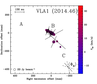
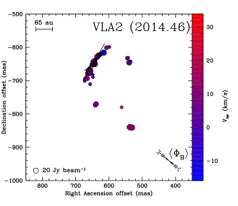
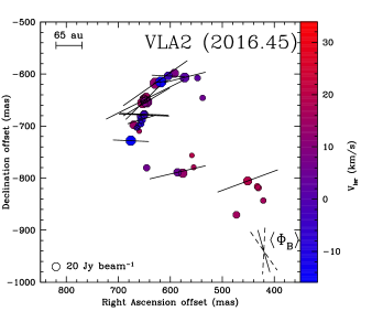
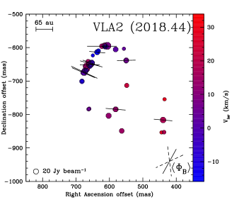
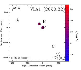
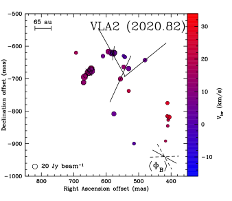
Figure 13: A close-up view of the 22 GHz H₂O maser features detected around the radio sources VLA 1 (left panels) and VLA 2 (right panels) in epochs 2014.46 (top panels), 2016.45, 2018.44, and 2020.82 (bottom panels). The reference positions are reported in Table 2. The letters A, B, and C indicate the position of the three maser groups identified around VLA 1 by S+11a and they are reported here only for reference. The octagonal symbols are the identified maser features scaled logarithmically according to their peak intensity (Tables 10-17). Maser LSR radial velocities are indicated by color (the assumed systemic velocity of the region is $V_{\rm{lsr}}=+10.0$ km s^-1; Shepherd et al. 2003). The linear polarization vectors, scaled logarithmically according to the polarization fraction $P_{\rm{l}}$, are overplotted. In the bottom-right corner of all panels the error-weighted orientation of the magnetic field ($\langle\Phi_{\rm{B}}\rangle$) is also reported; the two dashed segments indicate the uncertainties.

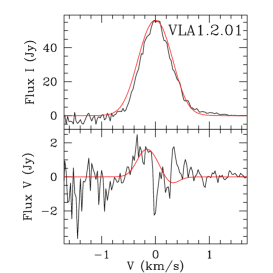
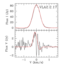
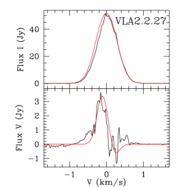
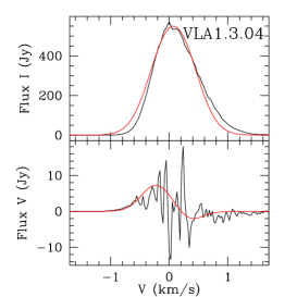
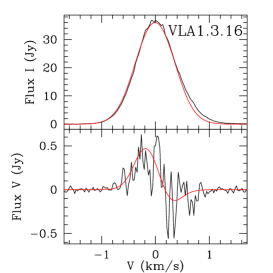
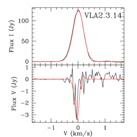
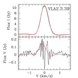
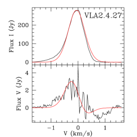
Figure 14: Total intensity spectra (I, upper panel) and circular polarization intensity spectra (V, lower panel) for the H₂O masers VLA1.2.01, VLA2.2.17, VLA2.2.27, VLA1.3.04, VLA1.3.16, VLA2.3.14, VLA2.3.39, and VLA2.4.27 (see Tables 12, 13, 14, 15, and 17). The thick red lines are the best-fit models of I and V emission obtained using the outputs of the FRTM code for 22 GHz H₂O masers (see Sect. 2), in particular these models are used to fit the spectra (for more details see S+11a). The maser features were centered on zero velocity.

Table 8: Parameters of all the 22 GHz H₂O maser features detected around VLA1 (epoch 2014.46).

(1)	(2)	(3)	(4)	(5)	(6)	(7)	(8)	(9)	(10)	(11)	(12)	(13)	(14)
Maser	RA	Dec	Zone	Peak	$V_{\rm{lsr}}$	$\Delta v\rm{{}_{L}}$	$P_{\rm{l}}$	$\chi$	$\Delta V_{\rm{i}}$	$T_{\rm{b}}\Delta\Omega$	$P_{\rm{V}}$	$B_{||}$	$\theta$
feature	offset	offset		Intensity (I)
	(mas)	(mas)		(Jy/beam)	(km/s)	(km/s)	(%)	(∘)	(km/s)	(log K sr)	($\%$)	(mG)	(∘)
VLA1.1.01	-101.803	-153.618	-	$0.43\pm 0.03$	8.37	$0.38$	$-$	$-$	$-$	$-$	$-$	$-$	$-$
VLA1.1.02	-101.761	-156.307	-	$0.57\pm 0.04$	8.48	$0.44$	$-$	$-$	$-$	$-$	$-$	$-$	$-$
VLA1.1.03	-64.879	-93.826	-	$2.59\pm 0.17$	12.77	$0.52$	$15.6\pm 2.0$	$+48\pm 3$	$<0.4$	$8.5^{+0.6}_{-1.1}$	$-$	$-$	$90^{+7}_{-7}$
VLA1.1.04	-31.619	-19.016	-	$15.85\pm 0.15$	12.61	$2.88$	$10.1\pm 2.5$	$-62\pm 1$	$2.7^{+0.4}_{-0.3}$	$7.0^{+1.3}_{-1.1}$	$-$	$-$	$90^{+13}_{-13}$
VLA1.1.05	-28.672	-99.377	-	$86.37\pm 1.06$	10.61	$2.31$	$2.3\pm 0.6$	$-25\pm 4$	$0.5$	$9.4^{+0.2}_{-0.1}$	$-$	$-$	$90^{+17}_{-17}$
VLA1.1.06	-24.588	-99.083	-	$8.37\pm 0.34$	11.35	$1.45$	$-$	$-$	$-$	$-$	$-$	$-$	$-$
VLA1.1.07	-23.703	-12.516	-	$74.21\pm 0.79$	10.98	$0.58$	$-$	$-$	$-$	$-$	$-$	$-$	$-$
VLA1.1.08	-14.778	-1.484	-	$23.15\pm 0.04$	8.63	$0.57$	$1.3\pm 0.1$	$-39\pm 3$	$3.2^{+0.2}_{-0.4}$	$9.1^{+0.6}_{-0.1}$	$-$	$-$	$75^{+14}_{-36}$
VLA1.1.09	-10.610	-10.700	-	$1.71\pm 0.02$	7.90	$2.81$	$-$	$-$	$-$	$-$	$-$	$-$	$-$
VLA1.1.10	-7.621	-6.420	-	$61.34\pm 0.35$	9.77	$2.10$	$-$	$-$	$-$	$-$	$-$	$-$	$-$
VLA1.1.11	-6.821	-9.647	-	$44.38\pm 0.13$	12.48	$1.22$	$0.7\pm 0.1$	$-45\pm 5$	$-$	$-$	$-$	$-$	$-$
VLA1.1.12	-5.810	-6.111	-	$34.60\pm 0.21$	9.56	$0.58$	$-$	$-$	$-$	$-$	$-$	$-$	$-$
VLA1.1.13	-4.084	-9.914	-	$0.54\pm 0.01$	16.77	$3.61$	$-$	$-$	$-$	$-$	$-$	$-$	$-$
VLA1.1.14	1.684	1.221	-	$9.01\pm 0.20$	9.53	$0.87$	$-$	$-$	$-$	$-$	$-$	$-$	$-$
VLA1.1.15	0	0	-	$1205.52\pm 1.05$	10.45	$0.92$	$0.4\pm 0.1$	$-32\pm 5$	$-$	$-$	$-$	$-$	$-$
VLA1.1.16	2.779	-0.122	-	$49.67\pm 0.21$	13.03	$1.55$	$0.5\pm 0.1$	$-34\pm 5$	$2.9^{+0.1}_{-0.2}$	$8.7^{+0.5}_{-0.1}$	$-$	$-$	$80^{+10}_{-37}$
VLA1.1.17	11.662	7.095	-	$5.72\pm 0.04$	8.90	$1.65$	$-$	$-$	$-$	$-$	$-$	$-$	$-$
VLA1.1.18	12.673	8.083	-	$14.22\pm 0.10$	9.29	$1.08$	$-$	$-$	$-$	$-$	$-$	$-$	$-$
VLA1.1.19	16.251	11.299	-	$9.16\pm 0.26$	11.37	$0.97$	$-$	$-$	$-$	$-$	$-$	$-$	$-$
VLA1.1.20	16.378	10.674	-	$13.52\pm 0.02$	19.67	$1.87$	$0.7\pm 0.1$	$-41\pm 5$	$-$	$-$	$-$	$-$	$-$
VLA1.1.21	17.767	13.378	-	$8.08\pm 0.25$	11.37	$0.77$	$-$	$-$	$-$	$-$	$-$	$-$	$-$
VLA1.1.22	36.250	24.662	-	$21.39\pm 0.37$	9.79	$1.38$	$-$	$-$	$-$	$-$	$-$	$-$	$-$
VLA1.1.23	36.418	20.989	-	$15.00\pm 0.10$	12.27	$2.05$	$-$	$-$	$-$	$-$	$-$	$-$	$-$
VLA1.1.24	37.639	20.233	-	$62.51\pm 0.14$	12.58	$0.72$	$0.6\pm 0.1$	$-22\pm 4$	$3.8^{+0.1}_{-0.3}$	$7.6^{+0.5}_{-0.2}$	$-$	$-$	$80^{+10}_{-31}$
VLA1.1.25	38.397	21.591	-	$680.26\pm 0.61$	14.14	$1.36$	$0.6\pm 0.1$	$-35\pm 2$	$-$	$-$	$-$	$-$	$-$
VLA1.1.26	40.418	21.824	-	$134.29\pm 0.25$	13.19	$0.68$	$0.5\pm 0.1$	$-40\pm 4$	$4.2^{+0.1}_{-0.2}$	$8.7^{+0.3}_{-0.2}$	$-$	$-$	$86^{+4}_{-12}$
VLA1.1.27	40.460	22.739	-	$42.89\pm 0.24$	13.19	$0.83$	$1.3\pm 0.1$	$-23\pm 2$	$4.0^{+0.3}_{-0.3}$	$9.1^{+1.0}_{-3.1}$	$-$	$-$	$87^{+3}_{-23}$
VLA1.1.28	54.943	31.521	-	$3.67\pm 0.13$	12.50	$0.88$	$-$	$-$	$-$	$-$	$-$	$-$	$-$

Table 9: Parameters of all the 22 GHz H₂O maser features detected around VLA2 (epoch 2014.46).

(1)	(2)	(3)	(4)	(5)	(6)	(7)	(8)	(9)	(10)	(11)	(12)	(13)	(14)
Maser	RA	Dec	Zone	Peak	$V_{\rm{lsr}}$	$\Delta v\rm{{}_{L}}$	$P_{\rm{l}}$	$\chi$	$\Delta V_{\rm{i}}$	$T_{\rm{b}}\Delta\Omega$	$P_{\rm{V}}$	$B_{||}$	$\theta$
feature	offset	offset		Intensity (I)
	(mas)	(mas)		(Jy/beam)	(km/s)	(km/s)	(%)	(∘)	(km/s)	(log K sr)	($\%$)	(mG)	(∘)
VLA2.1.01	531.033	-840.988	3	$21.02\pm 0.13$	12.48	$0.66$	$-$	$-$	$-$	$-$	$-$	$-$	$-$
VLA2.1.02	535.453	-643.040	2	$0.89\pm 0.01$	5.87	$1.00$	$-$	$-$	$-$	$-$	$-$	$-$	$-$
VLA2.1.03	537.137	-839.603	3	$21.13\pm 0.25$	14.90	$0.65$	$-$	$-$	$-$	$-$	$-$	$-$	$-$
VLA2.1.04	539.369	-646.263	2	$5.87\pm 0.02$	4.26	$2.12$	$-$	$-$	$-$	$-$	$-$	$-$	$-$
VLA2.1.05	540.927	-646.011	2	$2.11\pm 0.01$	3.13	$0.66$	$-$	$-$	$-$	$-$	$-$	$-$	$-$
VLA2.1.06	541.979	-631.249	2	$0.27\pm 0.01$	6.29	$0.53$	$-$	$-$	$-$	$-$	$-$	$-$	$-$
VLA2.1.07	544.758	-632.530	2	$1.13\pm 0.02$	7.37	$0.56$	$-$	$-$	$-$	$-$	$-$	$-$	$-$
VLA2.1.08	545.895	-631.870	2	$0.22\pm 0.01$	6.21	$0.45$	$-$	$-$	$-$	$-$	$-$	$-$	$-$
VLA2.1.09	561.935	-779.900	3	$0.27\pm 0.01$	21.19	$0.66$	$-$	$-$	$-$	$-$	$-$	$-$	$-$
VLA2.1.10	598.985	-598.778	1	$0.49\pm 0.02$	7.21	$0.62$	$-$	$-$	$-$	$-$	$-$	$-$	$-$
VLA2.1.11	607.153	-600.987	1	$1.85\pm 0.09$	12.27	$0.59$	$-$	$-$	$-$	$-$	$-$	$-$	$-$
VLA2.1.12	615.784	-615.742	1	$14.16\pm 0.02$	-11.59	$0.55$	$-$	$-$	$-$	$-$	$-$	$-$	$-$
VLA2.1.13	617.426	-614.739	1	$0.26\pm 0.01$	-6.03	$0.79$	$-$	$-$	$-$	$-$	$-$	$-$	$-$
VLA2.1.14	622.226	-617.950	1	$0.72\pm 0.01$	1.52	$1.10$	$-$	$-$	$-$	$-$	$-$	$-$	$-$
VLA2.1.15	624.246	-620.457	1	$0.55\pm 0.01$	-0.74	$0.92$	$-$	$-$	$-$	$-$	$-$	$-$	$-$
VLA2.1.16	625.552	-621.185	1	$1.16\pm 0.01$	0.37	$0.78$	$-$	$-$	$-$	$-$	$-$	$-$	$-$
VLA2.1.17	629.846	-625.595	1	$0.75\pm 0.01$	2.34	$0.66$	$-$	$-$	$-$	$-$	$-$	$-$	$-$
VLA2.1.18	632.414	-623.024	1	$2.76\pm 0.02$	14.98	$0.45$	$-$	$-$	$-$	$-$	$-$	$-$	$-$
VLA2.1.19	634.351	-629.128	1	$1.02\pm 0.01$	6.11	$0.69$	$-$	$-$	$-$	$-$	$-$	$-$	$-$
VLA2.1.20	635.951	-628.952	1	$10.24\pm 0.02$	15.24	$0.43$	$-$	$-$	$-$	$-$	$-$	$-$	$-$
VLA2.1.21	638.561	-770.130	3	$5.25\pm 0.05$	8.90	$0.55$	$-$	$-$	$-$	$-$	$-$	$-$	$-$
VLA2.1.22	640.793	-772.827	3	$2.81\pm 0.01$	5.61	$0.53$	$-$	$-$	$-$	$-$	$-$	$-$	$-$
VLA2.1.23	642.687	-650.074	1	$14.99\pm 0.71$	10.08	$1.85$	$-$	$-$	$-$	$-$	$-$	$-$	$-$
VLA2.1.24	643.529	-640.629	1	$4.68\pm 0.15$	15.24	$0.42$	$4.6\pm 1.2$	$-31\pm 5$	$-$	$-$	$-$	$-$	$-$
VLA2.1.25	643.698	-645.699	1	$1.62\pm 0.01$	16.85	$0.52$	$-$	$-$	$-$	$-$	$-$	$-$	$-$
VLA2.1.26	644.245	-642.471	1	$25.15\pm 0.14$	15.27	$0.45$	$0.9\pm 0.2$	$-42\pm 6$	$1.6^{+0.1}_{-0.2}$	$8.9^{+0.3}_{-1.2}$	$-$	$-$	$79^{+11}_{-17}$
VLA2.1.27	645.213	-652.153	1	$2.48\pm 0.07$	9.19	$0.57$	$-$	$-$	$-$	$-$	$-$	$-$	$-$
VLA2.1.28	645.466	-647.984	1	$0.22\pm 0.01$	16.67	$0.44$	$-$	$-$	$-$	$-$	$-$	$-$	$-$
VLA2.1.29	645.887	-644.447	1	$25.57\pm 0.11$	15.40	$0.46$	$1.5\pm 0.7$	$-47\pm 4$	$1.6^{+0.1}_{-0.3}$	$9.2^{+0.3}_{-2.1}$	$-$	$-$	$79^{+11}_{-44}$
VLA2.1.30	645.971	-653.091	1	$0.99\pm 0.04$	8.56	$0.73$	$-$	$-$	$-$	$-$	$-$	$-$	$-$
VLA2.1.31	646.097	-646.828	1	$6.83\pm 0.22$	15.88	$0.48$	$1.4\pm 0.2$	$-41\pm 6$	$1.6^{+0.2}_{-0.2}$	$9.2^{+0.3}_{-1.2}$	$-$	$-$	$86^{+3}_{-13}$
VLA2.1.32	648.371	-689.751	1	$0.23\pm 0.13$	-3.85	$0.76$	$-$	$-$	$-$	$-$	$-$	$-$	$-$
VLA2.1.33	648.539	-682.083	1	$0.21\pm 0.01$	-5.51	$0.55$	$-$	$-$	$-$	$-$	$-$	$-$	$-$
VLA2.1.34	650.139	-651.642	1	$6.93\pm 0.06$	15.59	$0.46$	$-$	$-$	$-$	$-$	$-$	$-$	$-$
VLA2.1.35	656.202	-678.604	1	$3.28\pm 0.01$	0.68	$0.86$	$-$	$-$	$-$	$-$	$-$	$-$	$-$
VLA2.1.36	656.875	-710.316	1	$0.40\pm 0.01$	-6.14	$0.49$	$-$	$-$	$-$	$-$	$-$	$-$	$-$
VLA2.1.37	656.918	-668.846	1	$1.61\pm 0.04$	15.45	$0.50$	$-$	$-$	$-$	$-$	$-$	$-$	$-$
VLA2.1.38	656.918	-670.769	1	$31.70\pm 0.20$	15.09	$2.12$	$0.9\pm 0.1$	$-39\pm 9$	$1.9^{+0.1}_{-0.3}$	$8.9^{+0.5}_{-0.3}$	$-$	$-$	$79^{+12}_{-36}$
VLA2.1.39	660.580	-672.241	1	$17.93\pm 0.45$	14.56	$0.39$	$-$	$-$	$-$	$-$	$-$	$-$	$-$
VLA2.1.40	663.654	-678.890	1	$4.59\pm 0.35$	13.43	$0.38$	$-$	$-$	$-$	$-$	$-$	$-$	$-$
VLA2.1.41	665.380	-693.222	1	$4.19\pm 0.13$	12.48	$0.68$	$-$	$-$	$-$	$-$	$-$	$-$	$-$
VLA2.1.42	671.653	-695.343	1	$1.35\pm 0.02$	7.98	$0.62$	$-$	$-$	$-$	$-$	$-$	$-$	$-$
VLA2.1.43	673.295	-701.130	1	$0.30\pm 0.01$	5.05	$0.65$	$-$	$-$	$-$	$-$	$-$	$-$	$-$

Table 10: Parameters of all the 22 GHz H₂O maser features detected around VLA1 (epoch 2016.45).

(1)	(2)	(3)	(4)	(5)	(6)	(7)	(8)	(9)	(10)	(11)	(12)	(13)	(14)
Maser	RA	Dec	Zone	Peak	$V_{\rm{lsr}}$	$\Delta v\rm{{}_{L}}$	$P_{\rm{l}}$	$\chi$	$\Delta V_{\rm{i}}$	$T_{\rm{b}}\Delta\Omega$	$P_{\rm{V}}$	$B_{||}$	$\theta$
feature	offset	offset		Intensity (I)
	(mas)	(mas)		(Jy/beam)	(km/s)	(km/s)	(%)	(∘)	(km/s)	(log K sr)	($\%$)	(mG)	(∘)
VLA1.2.01	-18.441	1.366	-	$57.07\pm 1.42$	12.29	0.66	$2.2\pm 0.2$	$-72\pm 10$	$3.8^{+0.1}_{-0.5}$	$9.3^{+0.5}_{-1.6}$	$3.5$	$-676\pm 102$	$90^{+11}_{-11}$
VLA1.2.02	-11.915	-9.304	-	$0.29\pm 0.02$	16.40	0.76	$-$	$-$	$-$	$-$	$-$	$-$	$-$
VLA1.2.03	-9.052	-3.773	-	$659.23\pm 2.17$	9.48	0.66	$0.7\pm 0.1$	$-73\pm 4$	$3.9^{+0.2}_{-0.7}$	$9.2^{+0.4}_{-1.2}$	$-$	$-$	$-$
VLA1.2.04	-4.210	0.237	-	$13.25\pm 0.42$	7.82	1.99	$-$	$-$	$-$	$-$	$-$	$-$	$-$
VLA1.2.05	-3.873	0.980	-	$47.27\pm 0.64$	8.98	0.75	$1.3\pm 0.1$	$-76\pm 15$	$4.3^{+0.1}_{-0.6}$	$6.8^{+0.2}_{-0.7}$	$-$	$-$	$90^{+11}_{-11}$
VLA1.2.06	-1.810	18.555	-	$134.08\pm 1.61$	10.14	0.70	$-$	$-$	$-$	$-$	$-$	$-$	$-$
VLA1.2.07	0	0	-	$1619.87\pm 4.42$	10.92	1.19	$0.8\pm 0.1$	$-59\pm 3$	$-$	$-$	$-$	$-$	$-$
VLA1.2.08	11.452	12.955	-	$25.57\pm 0.86$	9.27	1.14	$-$	$-$	$-$	$-$	$-$	$-$	$-$
VLA1.2.09	26.945	32.818	-	$330.99\pm 2.28$	10.35	0.58	$-$	$-$	$-$	$-$	$-$	$-$	$-$
VLA1.2.10	33.892	21.893	-	$24.05\pm 0.72$	13.43	3.68	$-$	$-$	$-$	$-$	$-$	$-$	$-$
VLA1.2.11	35.366	44.006	-	$10.46\pm 0.23$	9.00	1.21	$-$	$-$	$-$	$-$	$-$	$-$	$-$
VLA1.2.12	36.124	22.461	-	$35.42\pm 1.19$	9.29	0.81	$-$	$-$	$-$	$-$	$-$	$-$	$-$
VLA1.2.13	37.723	21.629	-	$412.53\pm 1.48$	12.69	1.10	$1.0\pm 0.1$	$-65\pm 16$	$-$	$-$	$-$	$-$	$-$
VLA1.2.14	38.144	21.221	-	$98.05\pm 4.33$	10.82	1.31	$1.2\pm 0.4$	$-11\pm 14$	$-$	$-$	$-$	$-$	$-$
VLA1.2.15	41.765	25.604	-	$28.31\pm 0.73$	13.40	0.80	$-$	$-$	$-$	$-$	$-$	$-$	$-$
VLA1.2.16	42.691	0.790	-	$0.24\pm 0.02$	2.68	0.49	$-$	$-$	$-$	$-$	$-$	$-$	$-$
VLA1.2.17	47.112	24.559	-	$150.64\pm 0.68$	13.51	1.05	$2.1\pm 0.5$	$-56\pm 3$	$-$	$-$	$-$	$-$	$-$
VLA1.2.18	48.923	25.745	-	$35.99\pm 0.84$	13.56	0.91	$-$	$-$	$-$	$-$	$-$	$-$	$-$
VLA1.2.19	49.301	24.933	-	$4.04\pm 0.64$	15.72	1.05	$-$	$-$	$-$	$-$	$-$	$-$	$-$
VLA1.2.20	155.146	73.784	-	$3.72\pm 0.21$	13.64	1.09	$-$	$-$	$-$	$-$	$-$	$-$	$-$

Table 11: Parameters of all the 22 GHz H₂O maser features detected around VLA2 (epoch 2016.45).

(1)	(2)	(3)	(4)	(5)	(6)	(7)	(8)	(9)	(10)	(11)	(12)	(13)	(14)
Maser	RA	Dec	Zone	Peak	$V_{\rm{lsr}}$	$\Delta v\rm{{}_{L}}$	$P_{\rm{l}}$	$\chi$	$\Delta V_{\rm{i}}$	$T_{\rm{b}}\Delta\Omega$	$P_{\rm{V}}$	$B_{||}$	$\theta$
feature	offset	offset		Intensity (I)
	(mas)	(mas)		(Jy/beam)	(km/s)	(km/s)	(%)	(∘)	(km/s)	(log K sr)	($\%$)	(mG)	(∘)
VLA2.2.01	420.978	-843.044	4	$0.77\pm 0.02$	16.40	0.51	$-$	$-$	$-$	$-$	$-$	$-$	$-$
VLA2.2.02	421.399	-843.182	4	$0.76\pm 0.02$	16.50	0.55	$-$	$-$	$-$	$-$	$-$	$-$	$-$
VLA2.2.03	430.619	-818.573	4	$1.21\pm 0.02$	18.59	0.82	$-$	$-$	$-$	$-$	$-$	$-$	$-$
VLA2.2.04	432.598	-816.361	4	$1.17\pm 0.02$	20.67	0.71	$-$	$-$	$-$	$-$	$-$	$-$	$-$
VLA2.2.05	451.207	-805.458	4	$9.17\pm 0.04$	19.40	0.63	$1.6\pm 0.3$	$-70\pm 8$	$3.9^{+0.2}_{-0.3}$	$9.3^{+0.1}_{-2.3}$	$-$	$-$	$82^{+6}_{-12}$
VLA2.2.06	472.848	-870.491	3	$2.55\pm 0.17$	15.51	0.60	$-$	$-$	$-$	$-$	$-$	$-$	$-$
VLA2.2.07	537.853	-645.912	2	$0.68\pm 0.02$	5.63	0.80	$-$	$-$	$-$	$-$	$-$	$-$	$-$
VLA2.2.08	547.705	-607.678	2	$1.01\pm 0.02$	2.29	0.43	$-$	$-$	$-$	$-$	$-$	$-$	$-$
VLA2.2.09	555.073	-779.221	3	$0.44\pm 0.02$	17.27	0.65	$-$	$-$	$-$	$-$	$-$	$-$	$-$
VLA2.2.10	558.609	-756.298	3	$0.31\pm 0.03$	19.51	0.49	$-$	$-$	$-$	$-$	$-$	$-$	$-$
VLA2.2.11	572.419	-606.586	2	$21.72\pm 0.08$	1.71	0.54	$1.1\pm 0.2$	$-76\pm 10$	$3.6^{+0.1}_{-0.5}$	$9.0^{+0.8}_{-0.3}$	$-$	$-$	$76^{+15}_{-34}$
VLA2.2.12	575.913	-790.714	3	$10.59\pm 0.52$	13.45	0.61	$-$	$-$	$-$	$-$	$-$	$-$	$-$
VLA2.2.13	586.144	-788.815	3	$4.67\pm 0.02$	4.87	0.71	$1.4\pm 0.2$	$-77\pm 9$	$-$	$-$	$-$	$-$	$-$
VLA2.2.14	592.038	-598.564	1	$10.02\pm 0.25$	8.08	0.61	$-$	$-$	$-$	$-$	$-$	$-$	$-$
VLA2.2.15	604.037	-603.630	1	$7.59\pm 0.04$	-3.85	0.81	$0.9\pm 0.1$	$+87\pm 7$	$4.0^{+0.1}_{-0.2}$	$6.1^{+1.6}_{-0.1}$	$-$	$-$	$90^{+13}_{-13}$
VLA2.2.16	618.310	-615.192	1	$73.11\pm 0.28$	-13.88	0.68	$0.6\pm 0.1$	$-82\pm 5$	$4.2^{+0.1}_{-0.6}$	$8.7^{+0.1}_{-1.5}$	$-$	$-$	$90^{+30}_{-30}$
VLA2.2.17	629.004	-617.607	1	$84.57\pm 0.94$	12.11	0.65	$2.2\pm 0.4$	$-55\pm 5$	$3.5^{+0.1}_{-0.6}$	$9.4^{+0.4}_{-2.0}$	$4.9$	$-1498\pm 225$	$81^{+9}_{-10}$
VLA2.2.18	645.508	-780.159	3	$1.61\pm 0.02$	5.87	0.66	$-$	$-$	$-$	$-$	$-$	$-$	$-$
VLA2.2.19	645.718	-653.431	1	$90.99\pm 0.40$	8.71	0.53	$1.3\pm 0.6$	$-59\pm 7$	$-$	$-$	$-$	$-$	$-$
VLA2.2.20	646.560	-644.295	1	$7.34\pm 0.14$	15.56	0.47	$-$	$-$	$-$	$-$	$-$	$-$	$-$
VLA2.2.21	647.908	-653.736	1	$30.24\pm 1.18$	9.69	0.55	$-$	$-$	$-$	$-$	$-$	$-$	$-$
VLA2.2.22	648.834	-648.983	1	$5.75\pm 0.07$	15.74	0.51	$2.7\pm 0.7$	$-63\pm 19$	$<0.4$	$8.5^{+0.5}_{-1.0}$	$-$	$-$	$90^{+19}_{-19}$
VLA2.2.23	650.181	-677.208	1	$4.29\pm 0.02$	-2.16	0.64	$1.2\pm 0.3$	$+88\pm 7$	$3.6^{+0.1}_{-0.6}$	$9.1^{+0.1}_{-2.1}$	$-$	$-$	$90^{+15}_{-15}$
VLA2.2.24	650.771	-678.692	1	$4.99\pm 0.04$	-3.85	0.63	$1.2\pm 0.1$	$+88\pm 7$	$3.6^{+0.4}_{-0.1}$	$9.1^{+0.3}_{-0.1}$	$-$	$-$	$85^{+4}_{-9}$
VLA2.2.25	651.360	-646.961	1	$3.63\pm 0.12$	14.48	0.48	$-$	$-$	$-$	$-$	$-$	$-$	$-$
VLA2.2.26	651.907	-648.590	1	$2.83\pm 0.15$	14.40	0.79	$-$	$-$	$-$	$-$	$-$	$-$	$-$
VLA2.2.27	653.255	-655.125	1	$52.19\pm 0.23$	15.19	0.63	$1.2\pm 0.1$	$-45\pm 3$	$3.7^{+0.2}_{-0.2}$	$9.1^{+0.3}_{-0.1}$	$7.8$	$-2426\pm 364$	$85^{+6}_{-9}$
VLA2.2.28	655.570	-687.443	1	$7.77\pm 0.04$	-6.90	1.14	$0.8\pm 0.2$	$-77\pm 9$	$-$	$-$	$-$	$-$	$-$
VLA2.2.29	656.202	-695.667	1	$1.08\pm 0.02$	-8.88	0.59	$-$	$-$	$-$	$-$	$-$	$-$	$-$
VLA2.2.30	656.875	-689.842	1	$0.23\pm 0.02$	-5.11	0.86	$-$	$-$	$-$	$-$	$-$	$-$	$-$
VLA2.2.31	659.865	-709.724	1	$0.35\pm 0.02$	16.85	0.49	$-$	$-$	$-$	$-$	$-$	$-$	$-$
VLA2.2.32	659.612	-681.156	1	$0.23\pm 0.02$	0.71	0.83	$-$	$-$	$-$	$-$	$-$	$-$	$-$
VLA2.2.33	661.212	-698.853	1	$0.58\pm 0.02$	-4.61	0.88	$-$	$-$	$-$	$-$	$-$	$-$	$-$
VLA2.2.34	663.485	-703.415	1	$0.54\pm 0.02$	-4.59	0.76	$-$	$-$	$-$	$-$	$-$	$-$	$-$
VLA2.2.35	665.085	-703.720	1	$0.38\pm 0.03$	-3.61	0.62	$-$	$-$	$-$	$-$	$-$	$-$	$-$
VLA2.2.36	670.348	-697.502	1	$7.46\pm 0.30$	13.95	0.49	$-$	$-$	$-$	$-$	$-$	$-$	$-$
VLA2.2.37	676.032	-728.066	1	$>30$	-15.62	2.70	$0.9\pm 0.1$	$+88\pm 3$	$-$	$-$	$-$	$-$	$-$

Table 12: Parameters of all the 22 GHz H₂O maser features detected around VLA1 (epoch 2018.44).

(1)	(2)	(3)	(4)	(5)	(6)	(7)	(8)	(9)	(10)	(11)	(12)	(13)	(14)
Maser	RA	Dec	Zone	Peak	$V_{\rm{lsr}}$	$\Delta v\rm{{}_{L}}$	$P_{\rm{l}}$	$\chi$	$\Delta V_{\rm{i}}$	$T_{\rm{b}}\Delta\Omega$	$P_{\rm{V}}$	$B_{||}$	$\theta$
feature	offset	offset		Intensity (I)
	(mas)	(mas)		(Jy/beam)	(km/s)	(km/s)	(%)	(∘)	(km/s)	(log K sr)	($\%$)	(mG)	(∘)
VLA1.3.01	-68.500	-88.299	-	$2.13\pm 0.14$	12.90	0.82	$-$	$-$	$-$	$-$	$-$	$-$	$-$
VLA1.3.02	-27.156	-18.986	-	$36.76\pm 0.53$	10.74	0.92	$-$	$-$	$-$	$-$	$-$	$-$	$-$
VLA1.3.03	-0.463	-1.347	-	$17.56\pm 0.12$	11.82	1.29	$1.1\pm 0.1$	$-83\pm 2$	$<0.4$	$9.0^{+0.3}_{-0.3}$	$-$	$-$	$90^{+7}_{-7}$
VLA1.3.04	0	0	-	$446.25\pm 4.18$	8.63	1.10	$0.7\pm 0.1$	$-88\pm 6$	$3.6^{+0.1}_{-0.6}$	$9.1^{+0.4}_{-0.3}$	$1.6$	$-764\pm 115$	$68^{+18}_{-33}$
VLA1.3.05	2.147	-2.552	-	$2.08\pm 0.10$	11.98	1.45	$-$	$-$	$-$	$-$	$-$	$-$	$-$
VLA1.3.06	3.705	5.379	-	$283.86\pm 1.56$	9.58	1.14	$0.8\pm 0.1$	$+88\pm 5$	$3.9^{+0.2}_{-0.3}$	$9.1^{+0.8}_{-0.2}$	$-$	$-$	$\mathbf{63^{+11}_{-40}}$
VLA1.3.07	3.705	5.184	-	$265.98\pm 1.73$	9.56	1.15	$0.9\pm 0.1$	$+81\pm 6$	$3.8^{+0.1}_{-0.7}$	$9.4^{+0.4}_{-0.7}$	$-$	$-$	$\mathbf{62^{+3}_{-43}}$
VLA1.3.08	10.526	12.749	-	$21.66\pm 0.18$	7.77	1.16	$-$	$-$	$-$	$-$	$-$	$-$	$-$
VLA1.3.09	12.673	14.587	-	$11.87\pm 0.31$	11.45	0.80	$1.0\pm 0.1$	$-82\pm 3$	$1.5^{+0.1}_{-0.3}$	$9.0^{+0.3}_{-0.1}$	$-$	$-$	$85^{+5}_{-12}$
VLA1.3.10	19.872	18.551	-	$8.22\pm 0.14$	10.77	1.60	$-$	$-$	$-$	$-$	$-$	$-$	$-$
VLA1.3.11	21.514	45.429	-	$21.83\pm 0.16$	14.96	0.92	$10.6\pm 0.2$	$+86\pm 6$	$1.1^{+0.3}_{-0.3}$	$10.5^{+0.1}_{-0.3}$	$-$	$-$	$90^{+6}_{-6}$
VLA1.3.12	23.703	22.160	-	$67.31\pm 1.06$	9.98	1.01	$0.8\pm 0.3$	$+88\pm 7$	$3.2^{+0.1}_{-0.5}$	$8.9^{+0.2}_{-1.9}$	$-$	$-$	$90^{+41}_{-41}$
VLA1.3.13	62.479	31.822	-	$7.38\pm 0.18$	13.59	1.88	$-$	$-$	$-$	$-$	$-$	$-$	$-$
VLA1.3.14	63.532	63.618	-	$4.04\pm 0.31$	11.32	0.93	$-$	$-$	$-$	$-$	$-$	$-$	$-$
VLA1.3.15	63.827	65.319	-	$48.05\pm 0.57$	10.66	0.94	$1.1\pm 0.1$	$-86\pm 7$	$2.7^{+0.2}_{-0.2}$	$9.0^{+0.5}_{-0.3}$	$-$	$-$	$82^{+7}_{-13}$
VLA1.3.16	65.721	32.665	-	$29.64\pm 0.23$	13.30	1.10	$0.9\pm 0.1$	$-88\pm 4$	$3.6^{+0.1}_{-0.5}$	$8.9^{+0.3}_{-0.2}$	$1.6$	$-733\pm 113$	$82^{+7}_{-13}$
VLA1.3.17	81.467	32.475	-	$4.71\pm 0.39$	11.09	0.82	$-$	$-$	$-$	$-$	$-$	$-$	$-$
VLA1.3.18	84.120	31.231	-	$33.10\pm 0.42$	11.11	0.80	$1.1\pm 0.1$	$-85\pm 4$	$1.6^{+0.1}_{-0.4}$	$9.0^{+0.4}_{-0.1}$	$-$	$-$	$82^{+8}_{-31}$
VLA1.3.19	86.856	31.273	-	$11.23\pm 0.55$	10.80	0.87	$1.7\pm 0.1$	$-88\pm 7$	$1.8^{+0.1}_{-0.3}$	$9.3^{+0.3}_{-0.1}$	$-$	$-$	$78^{+1}_{-7}$
VLA1.3.20	94.814	42.259	-	$18.33\pm 0.22$	13.38	0.99	$1.0\pm 0.1$	$-88\pm 6$	$2.8^{+0.2}_{-0.2}$	$9.0^{+0.2}_{-0.2}$	$-$	$-$	$84^{+6}_{-11}$

Table 13: Parameters of all the 22 GHz H₂O maser features detected around VLA2 (epoch 2018.44).

(1)	(2)	(3)	(4)	(5)	(6)	(7)	(8)	(9)	(10)	(11)	(12)	(13)	(14)
Maser	RA	Dec	Zone	Peak	$V_{\rm{lsr}}$	$\Delta v\rm{{}_{L}}$	$P_{\rm{l}}$	$\chi$	$\Delta V_{\rm{i}}$	$T_{\rm{b}}\Delta\Omega$	$P_{\rm{V}}$	$B_{||}$	$\theta$
feature	offset	offset		Intensity (I)
	(mas)	(mas)		(Jy/beam)	(km/s)	(km/s)	(%)	(∘)	(km/s)	(log K sr)	($\%$)	(mG)	(∘)
VLA2.3.01	434.956	-754.345	4	$0.04\pm 0.01$	28.23	0.55	$-$	$-$	$-$	$-$	$-$	$-$	$-$
VLA2.3.02	436.429	-852.776	4	$1.06\pm 0.02$	18.59	0.73	$-$	$-$	$-$	$-$	$-$	$-$	$-$
VLA2.3.03	439.334	-816.387	4	$15.90\pm 0.06$	17.88	0.75	$1.2\pm 01$	$+85\pm 3$	$2.7^{+0.2}_{-0.5}$	$9.4^{+0.5}_{-0.6}$	$-$	$-$	$70^{+15}_{-36}$
VLA2.3.04	443.923	-853.413	4	$0.04\pm 0.01$	27.59	0.77	$-$	$-$	$-$	$-$	$-$	$-$	$-$
VLA2.3.05	548.252	-713.097	2	$2.18\pm 0.02$	22.25	0.60	$-$	$-$	$-$	$-$	$-$	$-$	$-$
VLA2.3.06	549.642	-638.168	2	$5.95\pm 0.03$	6.27	0.62	$1.2\pm 0.1$	$-89\pm 4$	$2.5^{+0.2}_{-0.2}$	$8.7^{+0.5}_{-1.0}$	$-$	$-$	$90^{+13}_{-13}$
VLA2.3.07	549.894	-639.736	2	$2.55\pm 0.03$	5.92	0.62	$-$	$-$	$-$	$-$	$-$	$-$	$-$
VLA2.3.08	556.546	-603.367	2	$0.58\pm 0.01$	3.53	0.50	$-$	$-$	$-$	$-$	$-$	$-$	$-$
VLA2.3.09	563.156	-848.869	3	$4.85\pm 0.13$	14.69	0.56	$-$	$-$	$-$	$-$	$-$	$-$	$-$
VLA2.3.10	581.302	-784.256	3	$6.26\pm 0.15$	14.80	0.94	$1.3\pm 0.2$	$+85\pm 11$	$3.4^{+0.2}_{-0.3}$	$6.0^{+2.0}_{-0.2}$	$-$	$-$	$90^{+11}_{-11}$
VLA2.3.11	581.429	-605.461	2	$6.23\pm 0.11$	1.79	0.49	$-$	$-$	$-$	$-$	$-$	$-$	$-$
VLA2.3.12	582.186	-784.851	3	$3.86\pm 0.17$	13.43	0.73	$-$	$-$	$-$	$-$	$-$	$-$	$-$
VLA2.3.13	602.311	-803.642	3	$9.25\pm 0.10$	12.80	0.63	$-$	$-$	$-$	$-$	$-$	$-$	$-$
VLA2.3.14	606.185	-594.807	1	$128.02\pm 1.00$	8.19	0.47	$-$	$-$	$-$	$-$	$2.9$	$+439\pm 66$	$-$
VLA2.3.15	607.827	-596.924	1	$0.40\pm 0.01$	-3.37	0.69	$-$	$-$	$-$	$-$	$-$	$-$	$-$
VLA2.3.16	613.005	-597.683	1	$2.62\pm 0.02$	-4.87	0.70	$-$	$-$	$-$	$-$	$-$	$-$	$-$
VLA2.3.17	613.089	-592.804	1	$4.30\pm 0.06$	12.38	0.53	$-$	$-$	$-$	$-$	$-$	$-$	$-$
VLA2.3.18	614.226	-598.274	1	$0.35\pm 0.02$	-5.66	1.08	$-$	$-$	$-$	$-$	$-$	$-$	$-$
VLA2.3.19	615.868	-593.662	1	$4.33\pm 0.07$	12.03	0.86	$-$	$-$	$-$	$-$	$-$	$-$	$-$
VLA2.3.20	616.036	-593.086	1	$2.23\pm 0.10$	13.72	0.65	$-$	$-$	$-$	$-$	$-$	$-$	$-$
VLA2.3.21	622.562	-595.924	1	$4.46\pm 0.12$	15.19	0.51	$2.3\pm 0.5$	$+90\pm 7$	$1.6^{+0.1}_{-0.4}$	$6.0^{+2.3}_{-0.2}$	$-$	$-$	$90^{+17}_{-17}$
VLA2.3.22	632.835	-609.512	1	$1.13\pm 0.01$	-13.88	0.79	$-$	$-$	$-$	$-$	$-$	$-$	$-$
VLA2.3.23	636.540	-613.735	1	$8.40\pm 0.04$	-15.85	0.58	$1.0\pm 0.1$	$+85\pm 4$	$0.8^{+0.1}_{-0.1}$	$10.5^{+0.1}_{-0.2}$	$-$	$-$	$\mathbf{14^{+37}_{-1}}$
VLA2.3.24	638.561	-614.048	1	$1.34\pm 0.02$	-11.77	1.02	$-$	$-$	$-$	$-$	$-$	$-$	$-$
VLA2.3.25	649.760	-623.409	1	$0.48\pm 0.01$	-12.09	0.62	$-$	$-$	$-$	$-$	$-$	$-$	$-$
VLA2.3.26	652.076	-644.253	1	$2.34\pm 0.02$	-4.24	0.67	$-$	$-$	$-$	$-$	$-$	$-$	$-$
VLA2.3.27	653.970	-646.782	1	$48.41\pm 0.19$	2.74	0.62	$1.1\pm 0.5$	$+70\pm 6$	$2.9^{+0.1}_{-0.5}$	$8.2^{+0.4}_{-1.7}$	$-$	$-$	$90^{+54}_{-54}$
VLA2.3.28	654.391	-648.689	1	$21.67\pm 0.12$	1.74	0.67	$1.6\pm 0.2$	$+75\pm 6$	$3.4^{+0.3}_{-0.5}$	$8.5^{+0.1}_{-2.28}$	$-$	$-$	$\mathbf{58^{+32}_{-46}}$
VLA2.3.29	658.138	-656.162	1	$1.68\pm 0.02$	-4.63	1.18	$-$	$-$	$-$	$-$	$-$	$-$	$-$
VLA2.3.30	658.560	-651.417	1	$61.99\pm 1.22$	9.74	0.67	$1.3\pm 1.2$	$+90\pm 27$	$3.6^{+0.1}_{-0.5}$	$6.2^{+0.7}_{-0.2}$	$-$	$-$	$90^{+62}_{-62}$
VLA2.3.31	659.023	-649.757	1	$15.90\pm 0.42$	10.56	0.47	$-$	$-$	$-$	$-$	$-$	$-$	$-$
VLA2.3.32	660.580	-782.860	3	$0.91\pm 0.02$	5.90	1.04	$-$	$-$	$-$	$-$	$-$	$-$	$-$
VLA2.3.33	662.349	-784.054	3	$0.98\pm 0.02$	5.21	0.67	$-$	$-$	$-$	$-$	$-$	$-$	$-$
VLA2.3.34	663.780	-642.242	1	$3.84\pm 0.11$	15.54	0.49	$-$	$-$	$-$	$-$	$-$	$-$	$-$
VLA2.3.35	666.938	-664.009	1	$7.33\pm 0.13$	7.21	0.60	$-$	$-$	$-$	$-$	$-$	$-$	$-$
VLA2.3.36	669.043	-668.186	1	$0.94\pm 0.02$	0.13	0.50	$-$	$-$	$-$	$-$	$-$	$-$	$-$
VLA2.3.37	669.885	-668.453	1	$4.71\pm 0.03$	-2.08	0.62	$-$	$-$	$-$	$-$	$-$	$-$	$-$
VLA2.3.38	670.390	-657.791	1	$1.94\pm 0.04$	14.24	0.40	$-$	$-$	$-$	$-$	$-$	$-$	$-$
VLA2.3.39	670.769	-655.510	1	$10.93\pm 0.13$	14.67	0.55	$-$	$-$	$-$	$-$	$1.5$	$-355\pm 69$	$-$
VLA2.3.40	675.232	-666.389	1	$3.59\pm 0.04$	8.74	0.91	$-$	$-$	$-$	$-$	$-$	$-$	$-$
VLA2.3.41	675.358	-673.714	1	$53.39\pm 0.40$	1.21	0.64	$2.2\pm 0.2$	$+65\pm 1$	$2.4^{+0.2}_{-0.4}$	$9.5^{+0.7}_{-1.2}$	$-$	$-$	$73^{+15}_{-34}$
VLA2.3.42	677.969	-675.056	1	$7.74\pm 0.22$	1.21	0.64	$1.8\pm 0.1$	$+67\pm 7$	$2.6^{+0.2}_{-0.2}$	$8.7^{+0.7}_{-1.0}$	$-$	$-$	$90^{+17}_{-17}$
VLA2.3.43	681.758	-700.119	1	$0.73\pm 0.01$	-7.95	3.32	$-$	$-$	$-$	$-$	$-$	$-$	$-$
VLA2.3.44	682.431	-700.844	1	$3.69\pm 0.02$	-7.87	1.14	$-$	$-$	$-$	$-$	$-$	$-$	$-$

Table 14: Parameters of all the 22 GHz H₂O maser features detected around VLA1 (epoch 2020.82).

(1)	(2)	(3)	(4)	(5)	(6)	(7)	(8)	(9)	(10)	(11)	(12)	(13)	(14)
Maser	RA	Dec	Zone	Peak	$V_{\rm{lsr}}$	$\Delta v\rm{{}_{L}}$	$P_{\rm{l}}$	$\chi$	$\Delta V_{\rm{i}}$	$T_{\rm{b}}\Delta\Omega$	$P_{\rm{V}}$	$B_{||}$	$\theta$
feature	offset	offset		Intensity (I)
	(mas)	(mas)		(Jy/beam)	(km/s)	(km/s)	(%)	(∘)	(km/s)	(log K sr)	($\%$)	(mG)	(∘)
VLA1.4.01	-8.378	-6.729	-	$0.37\pm 0.02$	19.03	0.55	$-$	$-$	$-$	$-$	$-$	$-$	$-$
VLA1.4.02	-5.894	-3.410	-	$114.86\pm 3.00$	8.84	1.22	$0.3\pm 0.1$	$-67\pm 19$	$2.6^{+0.1}_{-0.9}$	$10.6^{+0.1}_{-0.1}$	$-$	$-$	$\mathbf{54^{+2}_{-48}}$
VLA1.4.03	-5.852	-3.094	-	$0.31\pm 0.03$	25.91	3.36	$-$	$-$	$-$	$-$	$-$	$-$	$-$
VLA1.4.04	0	-2.228	-	$0.44\pm 0.01$	20.32	0.64	$-$	$-$	$-$	$-$	$-$	$-$	$-$
VLA1.4.05	0	0	-	$302.47\pm 2.59$	9.87	0.97	$0.1\pm 0.1$	$-5\pm 15$	$2.6^{+0.1}_{-0.9}$	$10.6^{+0.1}_{-0.1}$	$-$	$-$	$\mathbf{5^{+51}_{-1}}$
VLA1.4.06	38.271	40.607	-	$1.79\pm 0.02$	18.98	0.59	$-$	$-$	$-$	$-$	$-$	$-$	$-$
VLA1.4.07	40.923	44.167	-	$1.10\pm 0.03$	26.01	3.43	$-$	$-$	$-$	$-$	$-$	$-$	$-$
VLA1.4.08	43.786	43.541	-	$0.25\pm 0.02$	18.98	0.58	$-$	$-$	$-$	$-$	$-$	$-$	$-$
VLA1.4.09	46.523	47.241	-	$0.14\pm 0.02$	26.35	4.20	$-$	$-$	$-$	$-$	$-$	$-$	$-$
VLA1.4.10	46.817	47.165	-	$160.64\pm 1.83$	10.87	1.59	$-$	$-$	$-$	$-$	$-$	$-$	$-$

Table 15: Parameters of all the 22 GHz H₂O maser features detected around VLA2 (epoch 2020.82).

(1)	(2)	(3)	(4)	(5)	(6)	(7)	(8)	(9)	(10)	(11)	(12)	(13)	(14)
Maser	RA	Dec	Zone	Peak	$V_{\rm{lsr}}$	$\Delta v\rm{{}_{L}}$	$P_{\rm{l}}$	$\chi$	$\Delta V_{\rm{i}}$	$T_{\rm{b}}\Delta\Omega$	$P_{\rm{V}}$	$B_{||}$	$\theta$
feature	offset	offset		Intensity (I)
	(mas)	(mas)		(Jy/beam)	(km/s)	(km/s)	(%)	(∘)	(km/s)	(log K sr)	($\%$)	(mG)	(∘)
VLA2.4.01	406.368	-818.092	4	$0.42\pm 0.04$	27.14	0.61	$-$	$-$	$-$	$-$	$-$	$-$	$-$
VLA2.4.02	408.642	-826.874	4	$0.35\pm 0.02$	21.22	0.61	$-$	$-$	$-$	$-$	$-$	$-$	$-$
VLA2.4.03	410.242	-845.112	4	$0.37\pm 0.01$	18.43	0.65	$-$	$-$	$-$	$-$	$-$	$-$	$-$
VLA2.4.04	411.168	-775.082	4	$0.08\pm 0.01$	27.09	0.55	$-$	$-$	$-$	$-$	$-$	$-$	$-$
VLA2.4.05	411.926	-815.075	4	$0.05\pm 0.01$	27.22	0.52	$-$	$-$	$-$	$-$	$-$	$-$	$-$
VLA2.4.06	417.020	-891.735	4	$0.17\pm 0.02$	18.66	0.56	$-$	$-$	$-$	$-$	$-$	$-$	$-$
VLA2.4.07	480.258	-642.651	2	$1.57\pm 0.18$	5.63	1.60	$1.9\pm 0.6$	$-54\pm 14$	$2.6^{+0.4}_{-0.2}$	$8.4^{+0.4}_{-0.8}$	$-$	$-$	$90^{+38}_{-38}$
VLA2.4.08	514.318	-899.658	3	$0.46\pm 0.05$	1.10	1.29	$-$	$-$	$-$	$-$	$-$	$-$	$-$
VLA2.4.09	530.696	-737.679	2	$0.68\pm 0.02$	21.69	0.45	$-$	$-$	$-$	$-$	$-$	$-$	$-$
VLA2.4.10	531.033	-668.739	2	$8.68\pm 0.31$	5.31	0.54	$-$	$-$	$-$	$-$	$-$	$-$	$-$
VLA2.4.11	542.611	-633.331	2	$0.86\pm 0.05$	0.84	0.48	$-$	$-$	$-$	$-$	$-$	$-$	$-$
VLA2.4.12	546.231	-663.677	2	$1.85\pm 0.21$	12.77	0.55	$-$	$-$	$-$	$-$	$-$	$-$	$-$
VLA2.4.13	546.779	-629.688	2	$0.39\pm 0.05$	0.65	0.46	$-$	$-$	$-$	$-$	$-$	$-$	$-$
VLA2.4.14	556.209	-700.676	2	$10.30\pm 0.46$	15.40	0.55	$1.5\pm 0.5$	$-28\pm 17$	$2.9^{+0.4}_{-0.2}$	$8.3^{+0.4}_{-1.3}$	$-$	$-$	$90^{+31}_{-31}$
VLA2.4.15	574.355	-619.995	2	$6.80\pm 0.11$	9.29	2.71	$-$	$-$	$-$	$-$	$-$	$-$	$-$
VLA2.4.16	575.155	-621.258	2	$3.53\pm 0.09$	4.79	0.52	$-$	$-$	$-$	$-$	$-$	$-$	$-$
VLA2.4.17	576.418	-808.151	3	$3.66\pm 0.25$	5.00	0.60	$-$	$-$	$-$	$-$	$-$	$-$	$-$
VLA2.4.18	577.724	-621.490	2	$49.34\pm 0.51$	5.31	0.56	$0.2\pm 0.1$	$-10\pm 22$	$3.6^{+0.1}_{-0.5}$	$8.3^{+0.6}_{-1.0}$	$-$	$-$	$74^{+14}_{-36}$
VLA2.4.19	579.281	-621.262	2	$1.05\pm 0.02$	6.26	0.55	$-$	$-$	$-$	$-$	$-$	$-$	$-$
VLA2.4.20	583.281	-618.427	2	$6.63\pm 0.09$	5.34	0.55	$1.9\pm 0.7$	$+26\pm 27$	$2.7^{+0.3}_{-0.3}$	$8.3^{+0.4}_{-1.3}$	$-$	$-$	$90^{+54}_{-54}$
VLA2.4.21	584.039	-621.773	2	$0.14\pm 0.01$	-1.03	0.45	$-$	$-$	$-$	$-$	$-$	$-$	$-$
VLA2.4.22	584.081	-620.522	2	$50.25\pm 1.80$	9.21	0.46	$-$	$-$	$-$	$-$	$-$	$-$	$-$
VLA2.4.23	593.259	-616.524	2	$11.69\pm 0.23$	12.90	0.55	$-$	$-$	$-$	$-$	$-$	$-$	$-$
VLA2.4.24	610.184	-630.386	1	$1.47\pm 0.02$	6.47	0.61	$-$	$-$	$-$	$-$	$-$	$-$	$-$
VLA2.4.25	644.329	-668.327	1	$4.41\pm 0.23$	16.45	0.47	$-$	$-$	$-$	$-$	$-$	$-$	$-$
VLA2.4.26	644.792	-670.151	1	$0.76\pm 0.02$	16.93	0.37	$-$	$-$	$-$	$-$	$-$	$-$	$-$
VLA2.4.27	646.897	-675.522	1	$285.16\pm 4.13$	9.24	0.61	$-$	$-$	$-$	$-$	$1.3$	$-452\pm 68$	$-$
VLA2.4.28	646.939	-668.846	1	$19.99\pm 0.29$	16.29	0.55	$-$	$-$	$-$	$-$	$-$	$-$	$-$
VLA2.4.29	648.623	-671.463	1	$11.60\pm 0.26$	16.14	0.55	$-$	$-$	$-$	$-$	$-$	$-$	$-$
VLA2.4.30	653.507	-681.347	1	$8.14\pm 0.26$	14.87	0.96	$-$	$-$	$-$	$-$	$-$	$-$	$-$
VLA2.4.31	653.844	-679.752	1	$136.56\pm 1.49$	15.40	0.58	$0.15\pm 0.03$	$+40\pm 17$	$3.8^{+0.1}_{-0.3}$	$8.2^{+0.8}_{-0.3}$	$-$	$-$	$\mathbf{66^{+9}_{-43}}$
VLA2.4.32	653.844	-683.891	1	$2.40\pm 0.09$	14.19	0.42	$-$	$-$	$-$	$-$	$-$	$-$	$-$
VLA2.4.33	659.949	-680.241	1	$0.83\pm 0.08$	14.53	0.48	$-$	$-$	$-$	$-$	$-$	$-$	$-$
VLA2.4.34	663.022	-691.490	1	$3.26\pm 0.08$	10.26	2.85	$-$	$-$	$-$	$-$	$-$	$-$	$-$
VLA2.4.35	664.412	-690.178	1	$4.98\pm 0.07$	14.37	0.49	$-$	$-$	$-$	$-$	$-$	$-$	$-$
VLA2.4.36	667.611	-694.836	1	$47.57\pm 0.61$	13.45	0.70	$-$	$-$	$-$	$-$	$-$	$-$	$-$
VLA2.4.37	669.127	-710.930	1	$2.83\pm 0.21$	12.58	0.54	$-$	$-$	$-$	$-$	$-$	$-$	$-$
VLA2.4.38	670.221	-711.891	1	$5.64\pm 0.25$	12.55	0.38	$-$	$-$	$-$	$-$	$-$	$-$	$-$
VLA2.4.39	693.378	-620.022	1	$1.94\pm 0.08$	16.35	1.65	$-$	$-$	$-$	$-$	$-$	$-$	$-$

Appendix B Proper motion estimate of VLA 1.

To properly compare the positions of the H₂O maser features detected in the four EVN epochs with the continuum emissions of VLA 1 and VLA 2 observed in 2014, we must verify if the two massive YSOs have any proper motion within the region W75N(B). We report in Table 18 the absolute positions of the three massive YSOs VLA 1, VLA 2, and VLA 3 as measured at K-band with the VLA by Torrelles et al. (1997), Carrasco-González et al. (2015), and Rodríguez-Kamenetzky et al. (2020) in epochs 1996.96 and 2014.20. These positions were obtained by deconvolving the data of the two epochs with the same restoring circular beam of $0.\!\!^{\prime\prime}12$, as already done by Carrasco-González et al. (2015) and Rodríguez-Kamenetzky et al. (2020), and by fitting the emission with a Gaussian fit. Furthermore, as already done for the maser features of the last three EVN epochs, the positions of the three YSOs of epoch 2014.20 are also corrected assuming the proper motion of the region W75N(B) equal to the median proper motion measured for the 6.7 GHz CH₃OH maser features by Rygl et al. (2012), $\langle\mu_{\rm{\alpha}}\rangle=(-1.97\pm 0.10)\leavevmode\nobreak\ \rm{mas\leavevmode\nobreak\ yr^{-1}}$ and $\langle\mu_{\rm\delta}\rangle=(-4.16\pm 0.15)\leavevmode\nobreak\ \rm{mas\leavevmode\nobreak\ yr^{-1}}$.
We plot in the three panels of Fig. 15 the corrected positions of the three massive YSOs for the two epochs with the relative errors due to the thermal noise and to the Gaussian fit errors ($\Delta\alpha$, $\Delta\delta$), which are represented by squares, and with the restoring circular beam centered on each position (circles). We note from Fig. 15 that the positions of VLA 2 and VLA 3 in both epochs are consistent within the beam and from Table 17 that the position shifts between the two epochs are similar suggesting a possible systematic uncertainty. We cannot verify if this uncertainty is real or not because the structure of the two sources varied between the two epochs, in particular that of VLA 2. We can therefore assume that VLA 2 and VLA 3 did not move within W75N(B) over 17.24 years and that the positions of the H₂O maser features in VLA 2 in the last three EVN epochs do not need further corrections.
It is evident from both Fig. 15 and Table 17 that VLA 1 actually moved within W75N(B) between the two epochs. From the shift reported in Table 17 we measure a proper motion of VLA 1 within W75N(B) of $\langle\mu_{\rm{\alpha}}\rangle^{\rm{VLA\,1}}=(-6.3\pm 0.4)\leavevmode\nobreak\ \rm{mas\leavevmode\nobreak\ yr^{-1}}$ ($-38.9\pm 2.5$ km s^-1) and $\langle\mu_{\rm\delta}\rangle^{\rm{VLA\,1}}=(+5.0\pm 0.4)\leavevmode\nobreak\ \rm{mas\leavevmode\nobreak\ yr^{-1}}$ ($+30.9\pm 2.5$ km s^-1) along right ascension and declination, respectively. This motion might suggest that VLA 1 is a runaway protostar, but to verify this possibility it is necessary to carry-on ad-hoc multi epoch observations. Nevertheless, we decide to correct the positions of the H₂O maser features detected in the last three EVN epochs and associated with VLA 1 accordingly to the estimated proper motion of VLA 1.

Table 16: Absolute positions of the massive YSOs VLA 1 and VLA 2 in epochs 1996.96 and 2014.20.

(1)	(2)	(3)	(4)	(5)	(6)	(7)	(8)
epoch	$\alpha_{1950}$	$\delta_{1950}$	$\alpha_{2000}$	$\delta_{2000}$	$\Delta\alpha$	$\Delta\delta$	Ref.
	($\rm{{}^{h}:\leavevmode\nobreak\ ^{m}:\leavevmode\nobreak\ ^{s}}$)	($\rm{{}^{\circ}:\,^{\prime}:\,^{\prime\prime}}$)	($\rm{{}^{h}:\leavevmode\nobreak\ ^{m}:\leavevmode\nobreak\ ^{s}}$)	($\rm{{}^{\circ}:\,^{\prime}:\,^{\prime\prime}}$)	(mas)	(mas)
VLA 1
1996.96	20:36:50.0056	+42:26:58.507	20:38:36.4528	+42:37:34.850	7	7	(1)
2014.20			20:38:36.440	+42:37:34.865	0.2	0.2	(2)
2014.20*			20:38:36.443	+42:37:34.936			-
VLA 2
1996.96	20:36:50.0405	+42:26:58.783	20:38:36.4882	+42:37:34.128	7	7	(1)
2014.20			20:38:36.484	+42:37:34.086	1	1	(3)
2014.20*			20:38:36.487	+42:37:34.158			-
VLA 3
1996.96	20:36:50.0406	+42:26:58.095	20:38:36.4886	+42:37:33.440	1	1	(1)
2014.20			20:38:36.485	+42:37:33.400	0.1	0.1	(3)
2014.20*			20:38:36.488	+42:37:33.472			-

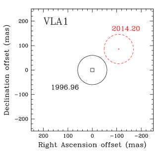
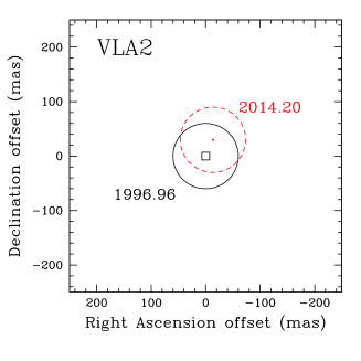
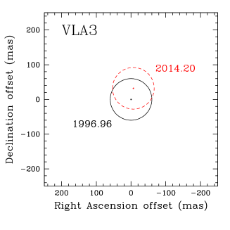
Figure 15: Comparison of the positions of the continuum emission at K-band of VLA 1 (left panel), VLA 2 (central panel), and VLA 3 (right panel) as observed in epoch 1996.96 (solid black; Torrelles et al. 1997) and epoch 2014.20 (dashed red; Carrasco-González et al. 2015; Rodríguez-Kamenetzky et al. 2020). The squares represent the uncertainties of the peaks positions (see Table 18) and the circles are the restoring circular beam of $0.\!\!^{\prime\prime}12$ used to properly compare the two epochs. Each panel is centered at the corresponding position of the YSO in epoch 1996.96 (see Table 18). The positions of epoch 2014.20 are corrected for the proper motion of the region W75N(B) as measured by Rygl et al. (2012), $\langle\mu_{\rm{\alpha}}\rangle=(-1.97\pm 0.10)\leavevmode\nobreak\ \rm{mas\leavevmode\nobreak\ yr^{-1}}$ and $\langle\mu_{\rm\delta}\rangle=(-4.16\pm 0.15)\leavevmode\nobreak\ \rm{mas\leavevmode\nobreak\ yr^{-1}}$.

Table 17: Shift of the positions of the three massive YSOs.

(1)	(2)	(3)
YSO	$\Delta(\alpha^{2014.20^{*}}-\alpha^{1996.96})$	$\Delta(\delta^{2014.20^{*}}-\delta^{1996.96})$
	(mas)	(mas)
VLA 1	$-108\pm 7$	$+86\pm 7$
VLA 2	$-13\pm 7$	$+30\pm 7$
VLA 3	$-7\pm 1$	$+32\pm 1$

References

- Alakoz et al. (2005) Alakoz, A. V., Slysh, V. I., Popov, M. V., & Val’tts, I. E. 2005, Astronomy Letters, 31, 375
- Anderson & Watson (1993) Anderson, N. & Watson, W. D. 1993, ApJ, 407, 620
- Carrasco-González et al. (2010) Carrasco-González, C., Rodríguez, L. F., Anglada, G., et al. 2010, Science, 330, 1209
- Carrasco-González et al. (2015) Carrasco-González, C., Torrelles, J. M., Cantó, J., et al. 2015, Science, 348, 114
- Colom et al. (2021) Colom, P., Ashimbaeva, N. T., Lekht, E. E., et al. 2021, Astronomy Reports, 65, 45
- Colom et al. (2018) Colom, P., Lekht, E. E., Pashchenko, M. I., Rudnitskii, G. M., & Tolmachev, A. M. 2018, Astronomy Reports, 62, 440
- Crutcher et al. (2010) Crutcher, R. M., Wandelt, B., Heiles, C., Falgarone, E., & Troland, T. H. 2010, ApJ, 725, 466
- Dall’Olio et al. (2019) Dall’Olio, D., Vlemmings, W. H. T., Persson, M. V., et al. 2019, A&A, 626, A36
- Davis et al. (1998) Davis, C. J., Moriarty-Schieven, G., Eislöffel, J., Hoare, M. G., & Ray, T. P. 1998, AJ, 115, 1118
- Elitzur et al. (1989) Elitzur, M., Hollenbach, D. J., & McKee, C. F. 1989, ApJ, 346, 983
- Fish et al. (2011) Fish, V. L., Gray, M., Goss, W. M., & Richards, A. M. S. 2011, MNRAS, 417, 555
- Fish et al. (2005) Fish, V. L., Reid, M. J., Argon, A. L., & Zheng, X.-W. 2005, ApJS, 160, 220
- Goddi et al. (2017) Goddi, C., Surcis, G., Moscadelli, L., et al. 2017, A&A, 597, A43
- Goldreich et al. (1973) Goldreich, P., Keeley, D. A., & Kwan, J. Y. 1973, ApJ, 179, 111
- Habing & Israel (1979) Habing, H. J. & Israel, F. P. 1979, ARA&A, 17, 345
- Harvey et al. (1977) Harvey, P. M., Campbell, M. F., & Hoffmann, W. F. 1977, ApJ, 211, 786
- Haschick et al. (1981) Haschick, A. D., Reid, M. J., Burke, B. F., Moran, J. M., & Miller, G. 1981, ApJ, 244, 76
- Hollenbach et al. (2013) Hollenbach, D., Elitzur, M., & McKee, C. F. 2013, ApJ, 773, 70
- Hunter et al. (1994) Hunter, T. R., Taylor, G. B., Felli, M., & Tofani, G. 1994, A&A, 284, 215
- Hutawarakorn et al. (2002) Hutawarakorn, B., Cohen, R. J., & Brebner, G. C. 2002, MNRAS, 330, 349
- Kang et al. (2016) Kang, J.-h., Byun, D.-Y., Kim, K.-T., et al. 2016, ApJS, 227, 17
- Kaufman & Neufeld (1996) Kaufman, M. J. & Neufeld, D. A. 1996, ApJ, 456, 250
- Keimpema et al. (2015) Keimpema, A., Kettenis, M. M., Pogrebenko, S. V., et al. 2015, Experimental Astronomy, 39, 259
- Kim et al. (2013) Kim, J.-S., Kim, S.-W., Kurayama, T., et al. 2013, ApJ, 767, 86
- Kim & Kim (2018) Kim, S.-W. & Kim, J.-S. 2018, in Astrophysical Masers: Unlocking the Mysteries of the Universe, ed. A. Tarchi, M. J. Reid, & P. Castangia, Vol. 336, 325–326
- Krasnov et al. (2015) Krasnov, V. V., Lekht, E. E., Rudnitskii, G. M., Pashchenko, M. I., & Tolmachev, A. M. 2015, Astronomy Letters, 41, 517
- Kuiper et al. (2016) Kuiper, R., Turner, N. J., & Yorke, H. W. 2016, ApJ, 832, 40
- Lekht (1994) Lekht, E. E. 1994, Astronomy Letters, 20, 395
- Lekht & Krasnov (2000) Lekht, E. E. & Krasnov, V. V. 2000, Astronomy Letters, 26, 38
- Lekht & Sorochenko (1984) Lekht, E. E. & Sorochenko, R. L. 1984, Pisma v Astronomicheskii Zhurnal, 10, 737
- Machida & Hosokawa (2020) Machida, M. N. & Hosokawa, T. 2020, MNRAS, 499, 4490
- Makin & Froebrich (2018) Makin, S. V. & Froebrich, D. 2018, ApJS, 234, 8
- Matsushita et al. (2018) Matsushita, Y., Sakurai, Y., Hosokawa, T., & Machida, M. N. 2018, MNRAS, 475, 391
- Minier et al. (2000) Minier, V., Booth, R. S., & Conway, J. E. 2000, A&A, 362, 1093
- Minier et al. (2001) Minier, V., Conway, J. E., & Booth, R. S. 2001, A&A, 369, 278
- Motte et al. (2018) Motte, F., Bontemps, S., & Louvet, F. 2018, ARA&A, 56, 41
- Myers et al. (2014) Myers, A. T., Klein, R. I., Krumholz, M. R., & McKee, C. F. 2014, MNRAS, 439, 3420
- Nedoluha & Watson (1992) Nedoluha, G. E. & Watson, W. D. 1992, ApJ, 384, 185
- Oliva & Kuiper (2022) Oliva, A. & Kuiper, R. 2022, arXiv e-prints, arXiv:2210.01492
- Palau et al. (2021) Palau, A., Zhang, Q., Girart, J. M., et al. 2021, ApJ, 912, 159
- Perley & Butler (2013) Perley, R. A. & Butler, B. J. 2013, ApJS, 206, 16
- Petrov et al. (2011) Petrov, L., Kovalev, Y. Y., Fomalont, E. B., & Gordon, D. 2011, AJ, 142, 35
- Qiu et al. (2008) Qiu, K., Zhang, Q., Megeath, S. T., et al. 2008, ApJ, 685, 1005
- Reid & Honma (2014) Reid, M. J. & Honma, M. 2014, ARA&A, 52, 339
- Rodríguez-Kamenetzky et al. (2020) Rodríguez-Kamenetzky, A., Carrasco-González, C., Torrelles, J. M., et al. 2020, MNRAS, 496, 3128
- Rodríguez-Kamenetzky et al. (2022) Rodríguez-Kamenetzky, A. R., Carrasco-González, C., Rodríguez, L. F., et al. 2022, ApJ, 931, L26
- Rosen & Krumholz (2020) Rosen, A. L. & Krumholz, M. R. 2020, AJ, 160, 78
- Rygl et al. (2012) Rygl, K. L. J., Brunthaler, A., Sanna, A., et al. 2012, A&A, 539, A79
- Sanhueza et al. (2021) Sanhueza, P., Girart, J. M., Padovani, M., et al. 2021, ApJ, 915, L10
- Sault (2012) Sault, R. 2012, EVLA Memo, 159
- Shepherd et al. (2003) Shepherd, D. S., Testi, L., & Stark, D. P. 2003, ApJ, 584, 882
- Slysh et al. (2010) Slysh, V. I., Alakoz, A. V., & Migenes, V. 2010, MNRAS, 404, 1121
- Slysh & Migenes (2006) Slysh, V. I. & Migenes, V. 2006, MNRAS, 369, 1497
- Surcis et al. (2011a) Surcis, G., Vlemmings, W. H. T., Curiel, S., et al. 2011a, A&A, 527, A48, (S+11a)
- Surcis et al. (2009) Surcis, G., Vlemmings, W. H. T., Dodson, R., & van Langevelde, H. J. 2009, A&A, 506, 757
- Surcis et al. (2011b) Surcis, G., Vlemmings, W. H. T., Torres, R. M., van Langevelde, H. J., & Hutawarakorn Kramer, B. 2011b, A&A, 533, A47
- Surcis et al. (2014) Surcis, G., Vlemmings, W. H. T., van Langevelde, H. J., et al. 2014, A&A, 565, L8, (S+14)
- Surcis et al. (2019) Surcis, G., Vlemmings, W. H. T., van Langevelde, H. J., Hutawarakorn Kramer, B., & Bartkiewicz, A. 2019, A&A, 623, A130
- Surcis et al. (2022) Surcis, G., Vlemmings, W. H. T., van Langevelde, H. J., Hutawarakorn Kramer, B., & Bartkiewicz, A. 2022, A&A, 658, A78
- Surcis et al. (2015) Surcis, G., Vlemmings, W. H. T., van Langevelde, H. J., et al. 2015, A&A, 578, A102
- Tan et al. (2014) Tan, J. C., Beltrán, M. T., Caselli, P., et al. 2014, in Protostars and Planets VI, ed. H. Beuther, R. S. Klessen, C. P. Dullemond, & T. Henning, 149
- Torrelles et al. (1997) Torrelles, J. M., Gómez, J. F., Rodríguez, L. F., et al. 1997, ApJ, 489, 744
- Torrelles et al. (2003) Torrelles, J. M., Patel, N. A., Anglada, G., et al. 2003, ApJ, 598, L115
- Vlemmings et al. (2006) Vlemmings, W. H. T., Diamond, P. J., van Langevelde, H. J., & Torrelles, J. M. 2006, A&A, 448, 597
- Wardle & Kronberg (1974) Wardle, J. F. C. & Kronberg, P. P. 1974, ApJ, 194, 249
- Westerhout (1958) Westerhout, G. 1958, Bull. Astron. Inst. Netherlands, 14, 215