The metal-weak Milky Way stellar disk hidden in the Gaia-Sausage-Enceladus debris: the APOGEE DR17 view.
Abstract
We have for the first time identified the early stellar disk in the Milky Way by using a combination of elemental abundances and kinematics. Using data from APOGEE DR17 and Gaia we select stars in the Mg-Mn-Al-Fe plane with elemental abundances indicative of accreted origin and find stars with both halo-like and disk-like kinematics. The stars with halo-like kinematics lie along a lower sequence in [Mg/Fe], while the stars with disk-like kinematics lie along a higher sequence. Through with asteroseismic observations, we determine the stars with halo-like kinematics are old, 9–11 Gyr and that the more evolved stellar disk is about 1–2 Gyr younger.
We show that the in situ fraction of stars on deeply bound orbits is not small, in fact the inner Galaxy likely harbours a genuine in-situ population together with an accreted one.
In addition, we show that the selection of Gaia-Sausage-Enceladus in the -plane is not very robust. In fact, radically different selection criteria give almost identical elemental abundance signatures for the accreted stars.
1 Introduction
The formation and evolution of the Milky Way can be studied via the ages, elemental abundances and kinematics of its stars (Freeman & Bland-Hawthorn, 2002). The stars present in the stellar components of the Galaxy are thought to have formed via two main processes: in situ formation and accretion. In situ stars would have formed in the body of the main progenitor of the galaxy and the accreted stars fin the galaxies that later merged with the main progenitor. The accreted stars would have chemical signatures different from those formed in situ since they have formed in shallower potential wells. However, some of the oldest stars formed in a Milky Way-like progenitor may occupy the same elemental abundance space as the accreted stars (Horta et al., 2022).
The Milky Way halo is thought to comprise stars formed in the early Milky Way as well as stars formed in nearby low-mass dwarf galaxies that have been accreted over time (Di Matteo et al., 2019; Helmi, 2020; Forbes, 2020; Hammer et al., 2023). Historically, these accreted stellar populations have been identified as spatial overdensities or kinematically associated stars (Helmi et al., 1999; Belokurov et al., 2006; Belokurov, 2013; Helmi, 2020) and have mainly been limited to mergers that have not yet dissolved into the Milky Way field populations. Following Gaia Data Release 1 (DR1, Gaia Collaboration et al., 2016a) and Data Release 2 (DR2, Gaia Collaboration et al., 2018a), substantial accreted material was identified in the Milky Way.
The most prominent, newly discovered stellar population is the Gaia-Sausage-Enceladus (Helmi et al., 2018; Belokurov et al., 2018; Myeong et al., 2019; Naidu et al., 2020). Apart from the Gaia-Sausage-Enceladus, several other debris have been identified using Gaia data (e.g. Myeong et al., 2019; Koppelman et al., 2019; Naidu et al., 2020). Most of these newly identified populations generally have metallicities lower than those of the Milky Way disk and bulge (see e.g. Malhan et al., 2022, Fig. 7 for some examples).
On a larger scale, it was found that the high velocity Milky Way halo has a dual sequence in the colour-magnitude diagram (Gaia Collaboration et al., 2018b). Helmi et al. (2018); Haywood et al. (2018); Sahlholdt et al. (2019a); Gallart et al. (2019) show that for stars with large transversal velocities (defined as km s-1), these two populations show different metallicity distribution functions, tentatively different elemental abundance trends, and different ages pointing to different origins, potentially we are seeing an in situ population (the red sequence) and an accreted population (the blue sequence). In addition, Belokurov et al. (2020) identified a structure they dubbed the Splash, which they take to be the result of the merger of the Gaia-Sausage-Enceladus. This merger perturbed stars in the existing stellar disk creating a heated component. Belokurov et al. (2020) identify the Splash as stars with km s-1 and [Fe/H] dex.
Di Matteo et al. (2019) argue that there is no in situ halo just an accreted one. In this interpretation, the two sequences in the halo colour-magnitude diagram are the cumulative accreted populations and the heated early disk. However, Amarante et al. (2020) provide simulations that show that it is feasible to create something akin to the Splash without any merger taking place. They argue for a formation of stars in a heated medium. It appears that observational data has not yet been sufficient to distinguish between different formation scenarios.
Although many accreted stellar populations have been identified in the Milky Way halo through their kinematics, the main criteria distinguishing stars as having formed outside the Milky Way is a difference in the elemental abundances. The elemental abundance ratios measured in the atmospheres of low-mass stars have long been used as a tool to probe the evolutionary history of galaxies. Not only does the abundance of individual elements increase over time as evolved stars contribute enriched material to the interstellar medium, but the star forming conditions of a given galaxy will affect the elemental abundance trends measured in its stellar populations.
Theoretically, it is well understood that the enrichment of -elements is dependent on the star formation rate (Matteucci, 2012). This is confirmed in observations of Local Group dwarf galaxies where star formation proceeds more slowly (Tolstoy et al., 2009). However, recently other elements have empirically been found to show significant differences in stars formed in high-mass or low-mass stellar systems. The APOGEE survey (Majewski et al., 2017) has provided aluminum abundance measurements for stars in the Milky Way and nearby dwarf galaxies. From this dataset, it has been shown that the accreted Gaia-Sausage-Enceladus stellar population and nearby dwarf galaxies have [Al/Fe] abundance ratios dex lower than the Milky Way disk across a large [Fe/H] range (e.g. Hasselquist et al., 2021; Horta et al., 2022).
Hawkins et al. (2015) and Das et al. (2020) suggest that the Mg-Mn-Al-Fe-plane could have high diagnostic power for identifying accreted populations in the Milky Way. Observational studies have found that many of the kinematically identified accreted stellar populations in the Milky Way lie within the proposed accreted region of this Mg-Mn-Al-Fe-plane (e.g. Feuillet et al., 2021; Horta et al., 2022). Initial attempts to understand this plane using chemical evolution models have found a difference in the expected distribution of low-mass Gaia-Sausage-Enceladus-like galaxies, present day dwarf galaxies and Milky Way-like galaxies. Horta et al. (2021); Fernandes et al. (2023) provide chemical evolution models in the Mg-Mn-Al-Fe-plane for these different types of galaxies.
In this paper we use the latest APOGEE dataset combined with astrometry from Gaia and the Mg-Mn-Al-Fe-plane to explore a subset of stars that have elemental abundances indicative of accreted or early Milky Way origin.
This paper is organised as follows: Section 2 describes our selection of data from APOGEE DR17 and Gaia. Section 4 discusses the chemical signatures of accreted populations, in particular the Mg-Mn-Al-Fe-plane and potential problems using this plane related to our shortcomings in deriving elemental abundances reliably. Section 3 defines our samples using the Mg-Mn-Al-Fe-plane while Sect. 5 explores the kinematic and chemical properties of specific samples. Section 6 attempts to date the different samples using ages available in the literature while Sect. 7 provides a discussion. The paper concludes with a summary in Sect. 8.
2 Data
We use data from the 17th Data Release (DR17) of the high-resolution spectroscopic SDSS APOGEE survey (Majewski et al., 2017; Abdurro’uf et al., 2022)111The data was retrieved from the SDSS-IV archive at https://www.sdss4.org/dr17/irspec/spectro_data/. combined with the Gaia Early Data Release 3 (Gaia EDR3, Gaia Collaboration et al., 2016b, 2021) astrometric data222For the purpose of the analysis present in this paper there is no difference between using EDR3 and DR3 for Gaia as the astrometric solution is the same. Gaia parameters additional to those provided by APOGEE were queried via the ESA archive https://gea.esac.esa.int/archive/. To ensure robust stellar parameters, elemental abundances, and kinematic measurements, we impose the selection criteria listed in Table 1.
| APOGEE DR17 | ||
| Flag | Criterium | |
| SNREV | 80 | |
| TEFF | 6000 | |
| TEFF | 4000 | |
| LOGG | 2.8 | |
| FE_H_FLAG | = | 0 |
| MG_FE_FLAG | = | 0 |
| MN_FE_FLAG | = | 0 |
| AL_FE_FLAG | = | 0 |
| STARFLAG | VERY_BRIGHT_NEIGHBOR or PERSIST_HIGH | |
| ASPCAPFLAG | STAR_BAD, CHI2_BAD, M_H_BAD, or CHI2_WARN | |
| EXTRATARG | DUPLICATE | |
| Gaia | ||
| Property | Criterium | |
| 0.2 | ||
| Additional selection for sample with no RC stars | ||
| Property | Criterium | |
| LOGG | 2 | |
| LOGG | 1 | |
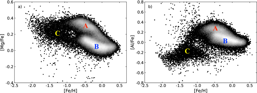
The sample is limited to giants to avoid an apparently anomalous feature in the [Al/Fe] vs [Fe/H] distribution of metal-rich dwarf stars. Although we focus mainly on lower metallicity stars in this work, aluminum is one of the four diagnostic elements used in our analysis and high data quality is important. The limits on effective temperature ensure only giants with reliable elemental abundance measurements are included. For more details on the APOGEE DR17 data quality see the SDSS DR17 documentation available on the web333https://www.sdss.org/dr17/ and a detailed discussion of DR16 in Jönsson et al. (2020). In addition, the sample is cleaned of stars in fields targeting known star clusters and dwarf galaxies. A full list of the field and program names removed can be found in App. A.1. This constitutes our full sample. In what follows we, following Weinberg et al. (2019), often limit the data set further to exclude red clump stars, i.e. .
The [Mg/Fe] and [Al/Fe] abundance distributions as a function of [Fe/H] of the full sample are shown in Fig. 1. In Fig. 1 we have indicated the classical thick disk sequence with a A in red and the classical thin with a B in blue. An additional low-[Mg/Fe] component can be seen at the lower metallicities, which has been identified by previous studies as a signature of an accreted population (Nissen & Schuster, 2010; Hayes et al., 2018; Haywood et al., 2018; Helmi et al., 2018). In Fig. 1 we indicate the position of this sequence with a C in yellow. These stars also have [Al/Fe] lower than the Milky Way disk, another potential signature of an accreted origin (Hawkins et al., 2015; Horta et al., 2021; Feuillet et al., 2021).
Full kinematics and 3D positions are calculated for the sample using Astropy (Astropy Collaboration et al., 2013, 2018) and galpy (Bovy, 2015). Input data used are Gaia astrometric measurements and magnitudes, photogeometric distances derived by Bailer-Jones et al. (2021), and APOGEE spectroscopic radial velocity measurements. We use the actionAngleStaeckel approximation (Bovy & Rix, 2013; Binney, 2012) with the MWPotential14 Milky Way potential (Bovy & Rix, 2013), delta of 0.4, and default values for all other parameters.
We estimated the uncertainties in the kinematics through a Monte Carlo analysis using 10 000 iterations. For each iteration, full kinematics were calculated using parameters drawn from an uncertainty distribution. A Gaussian distribution was used for the distance and radial velocity. For the RA proper motion and Dec proper motion, a multivariate Gaussian distribution was used accounting for the Gaia covariance in RA proper motion, Dec proper motion, and parallax as well as the uncertainty in the individual parameter. The uncertainty in the kinematic parameters for each star were taken to be the standard deviation in each parameter over the 10 000 iterations.
As the main focus of this paper in on a few subsamples, we calculate kinematic uncertainties for all of Sample I (see below) and a representative selection of Sample III. We find the largest kinematic uncertainties in stars on high-energy, low- orbits as these stars tend to be at larger distances. However, the typical uncertainties are less than 10% in all kinematic parameters and do not affect our conclusions. Effects of select kinematics are discussed where relevant in the text and the distributions of kinematic uncertainties are shown in Appendix B.
3 Defining and naming stellar samples selected in the Mg-Mn-Al-Fe-plane
In this section we make an empirical definition of the samples we wish to study. These definitions are based on the appearance of the data in the Mg-Mn-Al-Fe-plane. In Sect. 4 we will ascertained that the division of Milky Way stars into two samples using the Mg-Mn-Al-Fe-plane is robust against shortcomings in the elemental abundance analysis . We thus proceed with a discussion of how to best define and name our samples.
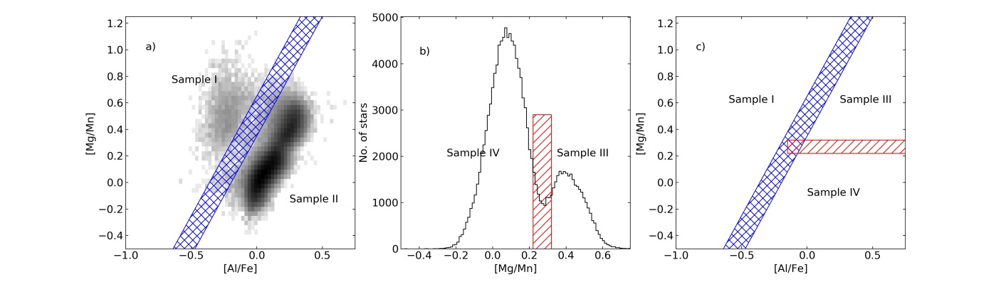
Figure 2 a) empirically defines our cut in the Mg-Mn-Al-Fe-plane, splitting the sample into two (Sample I and Sample II). The validity of the diagonal cut is extensively discussed in Sect. 4. Figure 2 b) shows a histogram of [Mg/Mn] for the stars in Sample II. We see a clear dip in the number counts (also visible in the 2D histogram in panel a). We define a cut such that stars with [Mg/Mn] 0.32 is one sample (Sample III) and stars with [Mg/Mn] 0.22 another (Sample IV). Table 2 summarises our empirical definitions of the samples. The current study is mainly concerned with Sample I and to some extent Sample III. We plan to return to the full Sample II and also Sample IV in other studies, but we show the full sample selection here for completeness. We are thus left with four different samples, where Sample III and IV are subsets of Sample II. Sample Ia and Ib are defined in Sect. 5.1.
Naming these samples is somewhat problematic. One option would be to call them halo, thick and thin disk or accreted and in-situ populations. However, it is likely that the thick disk (and halo) overlap to some larger or smaller extent with the Splash (Belokurov et al., 2020). Another option would be to follow Horta et al. (2021) and refer to the stars to the left of the diagonal cut as accreted stars. We are quite certain we will find some accreted stars there, but are all stars accreted?
Our aim is to investigate how these samples interact and how the Milky Way was assembled. By giving the samples names we may inadvertently guide our thinking. To avoid this we have opted to simply refer to the samples defined in the Mg-Mn-Al-Fe-plane as Sample I, II, III and IV (compare Fig. 2). If sub-samples are defined to these major samples, for example by imposing a kinematic constraint, they will be given a letter in addition to identify them (e.g. Sample Ia). The median uncertainty in for Sample I is 0.06. We note that we have left a substantial gap in the selection of Sample Ia and Ib.
| Name | Selection criteria |
|---|---|
| Sample I: | |
| S I | [Mg/Mn] [Al/Fe] |
| S Ia | plus |
| S Ib | plus |
| Sample II: | |
| S II | [Mg/Mn] [Al/Fe] |
| Sample III: | |
| S III | [Mg/Mn] [Al/Fe] |
| and [Mg/Mn] 0.32 | |
| Sample IV: | |
| S IV | [Mg/Mn] [Al/Fe] |
| and [Mg/Mn] 0.22 |
4 Chemical signatures of accreted stellar populations
It has long been understood that the elemental abundance ratios as observed in the stellar atmospheres of long-lived stars hold information about the conditions in the gas from which the stars formed (Lambert, 1989; McWilliam, 1997). By analysing the spectra of such stars we can trace the chemical evolution of a stellar population over time or we can use the abundance ratios as indications of the relative stellar ages. Different elements are released to the inter-stellar medium by stars with different masses and therefore on different timescales (see e.g. Arnett, 1996; Nomoto et al., 1997; Kobayashi et al., 2020). Comparing the elemental abundances therefore gives a timing of the events.
Stellar systems of different mass and gas densities will evolve on different timescales. This means that smaller galaxies, like the Magellanic Clouds and the dwarf spheroidal (dSph) galaxies, are expected to show different elemental abundance trend. This is born out by observations (see e.g. Tolstoy et al., 2009; Hasselquist et al., 2021). This in turn means that stellar populations accreted to the Milky Way should show elemental abundance trends that differ from those seen for stars formed in the main body of the Milky Way. Hereafter, we will refer to those stars as “in situ” stars while stars now present in the Milky Way that formed in (smaller) systems that have been accreted at some point onto the main body of the Milky Way will be referred to as “accreted”.
It is interesting to consider which elements will give us the best possibilities to identify accreted stellar populations. The best elements to use will depend on several factors, beyond those of purely chemical evolution concern, such as availability of atomic lines of sufficient strength (but not too strong), our ability to model the strengths of lines in the stellar spectra as a function of the elemental abundance, e.g., due to deviation from local thermal equilibrium.
Much focus has been attached to the -elements as it was early understood that they should show different trends depending on the star formation rate in the system (McWilliam, 1997, and references therein) and since such elements have atomic lines of good strength across the optical spectrum. Another focus has been the neutron-capture elements as they show distinct patterns for very metal-poor stars and for metal-poor stars in present day dSph galaxies (Bonifacio et al., 2009; Koch et al., 2013; Roederer et al., 2016). The neutron-capture elements are, however, difficult to study as in many stars the available lines are weak. Several of the spectral lines arising from these elements also have complex structures including hyper-fine-splitting and NLTE effects (see e.g. Battistini & Bensby, 2016, and references therein) making them difficult to analyse.
Here we follow upon the work of Hawkins et al. (2015) and explore the possibilities to use the elemental abundances of magnesium, manganese, aluminum and iron to identify accreted stars.
4.1 Exploring the Mg-Mn-Al-Fe-plane
Hawkins et al. (2015) and later Das et al. (2020) proposed to use the Mg-Mn-Al-Fe-plane to identify stellar populations formed in smaller systems and later accreted onto the main body of the Milky Way. Later works show that this works well for example in identifying the Gaia-Sausage-Enceladus members (Feuillet et al., 2021). To the best of our understanding, the works by Hawkins et al. (2015) and Das et al. (2020) were essentially empirical, inspired by the large and high quality dataset from APOGEE DR14. Horta et al. (2021) made a first theoretical illustration of how this plane can work to identify different stellar population. For completeness and because of the importance of these findings for our work we here repeat some of the arguments from Horta et al. (2021) for and against using the Mg-Mn-Al-Fe-plane to identify accreted stellar populations in the Milky Way.
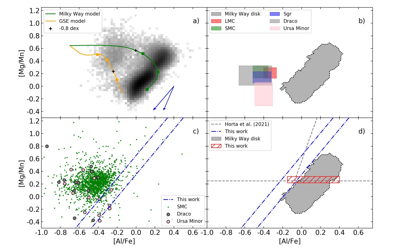
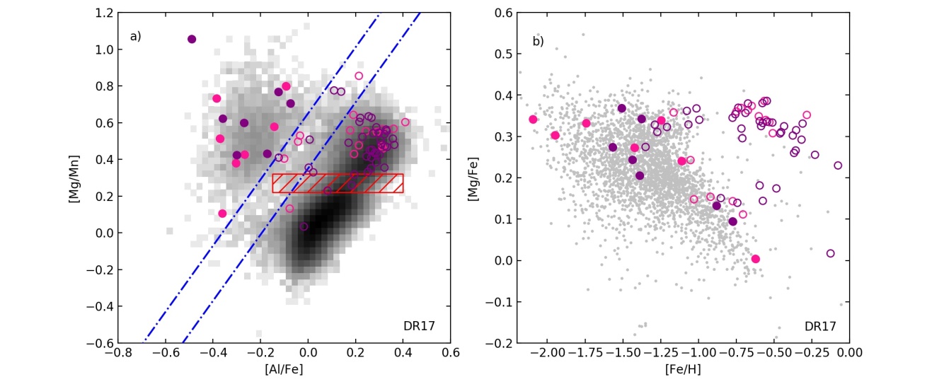
We start by exploring the Mg-Mn-Al-Fe-plane. Figure 3 a) shows the density map in this plane of the data selected in Sect. 2. We note that the stars are not evenly distributed. We see a lighter, round concentration centered at ([Al/Fe],[Mg/Mn]) = (–0.3,+0.5) dex and a more elongated structure to the right. In between these structures there is a clear depression in the number densities. We will, Hawkins et al. (2015) and Das et al. (2020) did, use this lack of stars as a natural place to separate traditional halo and disk stars. The stars in the structure to the right may also show two rather than a single structure with one round concentration at (0.3,0.45) and a more elongated structure below. We will return to these features in more detail in future studies.
The figure also shows evolutionary tracks for two different systems; the Milky Way and the Gaia-Sausage-Enceladus. The trends shown are replications from Horta et al. (2021), their Fig. 1. Horta et al. (2021) uses the Milky Way solar neighborhood chemical evolution model as their fiducial model (shown here in red) that is representative of in situ chemical evolution. The model shown in blue is tailored to represent the Gaia-Sausage-Enceladus progenitor. The latter then shows what an accreted stellar population may look like. For each model the following time stamps are indicated by filled circles: 300 Myr, 1 Gyr, and 5 Gyr. In addition the point when each model has reached a chemical enrichment of –0.8 dex is indicated. Further details on the model parameters can be found in Andrews et al. (2017) and Horta et al. (2021). As can be understood from these model predictions, the region to the left will inevitably include both accreted stars as well as in situ stars if the in situ population has a reasonably large amount of metal-poor stars. On the other hand if the in situ population mainly forms from gas that is already enriched then the region to the left will essentially be void of in situ stars.
Figure 3 b) shows where stars in different known systems fall. The Milky Way disk is shown by using the APOGEE DR17 data selected as disk stars for this study (shown as contours, see Fig. 4). In addition, data from APOGEE DR17 for the Large Magellanic Cloud (LMC), the Small Magellanic Cloud (SMC), the core and tidal stream of the Sagittarius (Sgr) dwarf spheroidal galaxy, and the Draco and Ursa Minor dSph galaxies are shown as coloured boxes. The selection of the stars in these galaxies are described in Appendix A.2. The centres of the boxes are the mean values of [Mg/Mn] and [Al/Fe] for the data for each galaxy and the size of the boxes is simply half of the standard deviation for each data set around their mean values. As can be seen, the Milky Way stellar disk (the heaviest system) has the highest [Al/Fe] values whilst lighter systems have lower [Al/Fe] values. Specifically, the SMC is lower in [Al/Fe] than the LMC. The Milky Way disk spans a large range in [Mg/Mn] while the other systems have a somewhat smaller range.
The smaller systems all have [Al/Fe] systematically lower than the Milky Way disk, indicating that it is not unreasonable to assume that stars from a systems that has formed in relative isolation and then accreted onto the main body of the Milky Way will be possible to identify thanks to their low [Al/Fe]. This is further supported by the models from Horta et al. (2021) and Fernandes et al. (2023) that show that a lighter system will reach a maximum [Al/Fe] value that is smaller than the main body of the Milky Way disk. See also Fernandes et al. (2023) for a full characterization of low-mass systems in APOGEE.
Figure 3 c) shows the full data-set used to calculate the boxes in Fig. 3 b) for SMC, and the Draco and Ursa Minor dSph galaxies. As can be seen scatter is relatively high for the two dSph galaxies whilst the data is more compactly distributed for SMC. The two lines illustrate the cut that we use to separate traditional halo from disk (Fig. 2). Dwarf galaxies surviving to this day are clearly on the left-hand side of these cuts and illustrate that we may reasonably assume to find accreted stars in those regions.
Figure 3 d) replicates the cuts used by Horta et al. (2021) to divide the plane into Accreted and In situ high- and low- stars (their nomenclature). We also show the cuts used in this study defined in Sect. 3. The main difference is that we divide the sample not considering any selection based on other elemental abundances (i.e. ). The near vertical cut that separate the samples differ somewhat between the two studies but the general idea is the same. In our selection, we also leave a gap in order to provide clean samples, while Horta et al. (2021) prefers a single cut with no gap. Horta et al. (2021) discuss how, based on their models, a Milky Way-sized galaxy will inevitably create some stars with high [Mg/Mn] and low [Al/Fe] that will contaminate any accreted population identified in the Mg-Mn-Al-Fe-plane (compare Fig. 3 a).
4.2 Comments on NLTE and 3D effects on the elemental abundances
In the vast majority of studies of stellar elemental abundances the abundances are derived under assumption of Local Thermal Equilibrium (LTE). Our understanding of how to treat departures from LTE (NLTE) has been growing for a long time and is now commonly implemented in small studies as well as in large spectroscopic surveys. Departures from LTE can have a significant effects, in particular when studying stars which span a wide range of [Fe/H]-values (see e.g. Bergemann et al., 2012; Lind et al., 2012). The stars in the samples we are studying are giant stars. For the most evolved stars, the assumption of plane parallel model atmospheres is also under question (Heiter & Eriksson, 2006) as well as the possibility that the stellar atmosphere is not homogenous but instead a full 3D modeling is necessary.
In large spectroscopic surveys it is difficult to take full account of NLTE and 3D effects, mainly because the calculation of these effects are time consuming. However, recently first instances of including e.g. departure from the LTE assumption have been performed in the 2nd and 3rd data release from the GALAH survey (Buder et al., 2018, 2021). In the future, more surveys will undoubtedly do so.
In APOGEE DR17, NLTE corrections have been applied to the magnesium abundance measurements following Osorio et al. (2020), but not for aluminum, iron, or manganese. This means that it is important for us to check whether the abundance measurements used in our study may be effected by NLTE and/or 3D effects to such a degree that our conclusions fail. Below we discuss possible effects on the two elemental abundance ratios that we consider in this work.
4.2.1 NLTE and 3D effects on [Al/Fe]
Nordlander & Lind (2017) studies NLTE and 3D effects on the derivation of [Al/Fe] in late type stars. They show that corrections can be substantial for some stars whilst for others the corrections are minor. In addition, the corrections vary significantly for a given star depending on which atomic lines are being used.
APOGEE uses three near-infrared Al I lines to derive the aluminum abundances. The lines in the APOGEE linelist by Shetrone et al. (2015); Smith et al. (2021) are listed as 16723.5, 16755, and 16768. Å. These are given as measured in vacuum, whilst the lines listed as APOGEE lines in Nordlander & Lind (2017) are given as 16718.9, 16750.5, and 16763.3 Å, which are measured in air. The line at 16750.5 Å (air) also has hyperfine splitting. This leads Nordlander & Lind (2017) to recommend that this line should not be used in derivation of aluminum abundances for metal-poor cool giant stars such as Arcturus.
For Arcturus, a red giant, with (/[Fe/H]) = (4247/1.59/–0.52), Nordlander & Lind (2017) find that average 3D and NLTE together gives a correction of about (–0.2,–0.3, -0.1 ) dex for the three lines used in APOGEE (as read from their Fig. 10). This should be compared to an average using all available lines across the optical and near-infrared stellar spectrum which give a difference of –0.13 dex (their Table 1). They also analyse HD 122563, another metal-poor giant, (/[Fe/H]) = (4608/1.61/–2.64). In this star the Al I lines are weak because the star is so metal-poor and they can therefore only analyse the lines at 16718.9 and 16750.5 Å (air). They find excellent agreement between the [Al/Fe] abundance in HD 122563 derived from these two lines and the blue UV line at 3961 Å, as well as an average difference of +0.09 dex in the sense 1D LTE - 3D NLTE (i.e. the value should be added to the 1D LTE value to achieve the corrected value).
Arcturus and HD 122563 span the full range of [Fe/H] for our sample and have and -values that are representative of our sample. The size of a 3D plus NLTE correction to [Al/H] abundance in Arcturus derived from near-infrared lines should be negative and the size about 0.2 dex. For HD 122563, which is much more metal-poor, the correction is also in the negative sense but less substantial, around 0.1 dex.
Although we do not have the possibility to apply line-by-line NLTE and 3D corrections to the data from APOGEE DR17 the discussion in the preceding text leads us to conclude that for the full sample the maximum corrections to [Al/H] from NLTE and 3D is no more than 0.2 dex (perhaps slightly more) and not less than 0.1 dex.
For optical spectra it is found that NLTE and 3D effects on derived iron abundances are small or negligible for stars around –1 dex and with surface gravities close to 1–2 (Bergemann et al., 2012; Lind et al., 2012; Amarsi et al., 2016). However, more recent studies indicate that the corrections could be larger than previously perceived (Amarsi et al., 2022). For iron lines in the wavelength region covered by APOGEE there exists no full 3D-NLTE calculation that can be trusted (Masseron et al., 2021). NLTE caclulation are readily available and show to be essentially non-existent for the stellar parameter range we are interested in. Taking these aspects into account we find that there is no need to consider NLTE-3D effects for iron for our sample. Hence, the effects for [Al/Fe] are the same as for [Al/H].
4.2.2 NLTE and 3D effects on [Mg/Mn]
For magnesium, we make use of the calculations by Bergemann et al. (2017) and Zhang et al. (2017) to estimate the size of the effects of departures from LTE, as well as 3D effects. Alexeeva et al. (2018) also study departures from LTE for magnesium but they do not include the near-infrared lines used in APOGEE DR17.
Zhang et al. (2017) study NLTE effects on derived magnesium abundances based on Mg I lines in the H-band. Their Table 3 shows that the maximum correction for 1D NLTE for red giant stars is 0.35 dex for [Mg/Fe]. Table 5 in Bergemann et al. (2017) shows that the difference between 1D LTE and 3D NLTE in [Mg/H] from NIR Mg lines is of the order zero.
Departures from 1D LTE for Mn was studied by Bergemann et al. (2019), who found that 3D NLTE Mn abundances derived from the Mn i lines used in APOGEE are, on average, significantly higher than those calculated in 1D LTE: for stars with ([Fe/H]) = (4500/2.0/–1) and (4500/2.0/–2.0) they find a correction of +0.3 and +0.35 dex, respectively (top panel in Fig. 17 in Bergemann et al., 2019).
Combining this information, we conclude that the [Mg/Mn] elemental abundances derived from the NIR Mn i lines used in APOGEE has a negative correction of up to 0.35 dex.
4.2.3 Summary: How well can stellar populations be separated in the Mg-Mn-Al-Fe-plane?
Based on the literature review provided in Sects. 4.2.1 and 4.2.2 we find that for a typical giant star in our sample the NLTE combined with 3D corrections amount to about –0.1 to –0.2 dex in [Al/Fe] and –0.35 dex in [Mg/Mn]. This implies a movement down and to the left in the Mg-Mn-Al-Fe-plane. The slope of the correction is roughly aligned with the empirical, diagonal cut we adopt to split our sample into two (see Fig. 3 and 2). This implies that although stars would collectively move within the diagram if the NLTE and 3D corrections were applied, in fact the gap between the two populations would remain.
We conclude that, in the case of the data selected in this study from APOGEE DR17, we can indeed make use of the Mg-Mn-Al-Fe-plane to separate accreted stars from those formed in the main body of the Galaxy. For individual stars there might be differences but for the populations as such it is sufficient to use the uncorrect elemental abundances from APOGEE DR17.
It is important to remember that this statement is valid for the stars selected for this study, i.e. stars on the Red Giant Branch (compare Table 1). Stars in other evolutionary stages may not be as readily separable and a fresh assessment should be made for each study taking exact atomic lines used in the derivation of the elemental abundances into account.
5 Kinematic properties and elemental abundances for Sample I and III
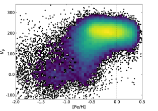
Figure 4 shows the density plot of as a function of [Fe/H] for our full sample. We see that the majority of the stars have a velocity compatible with that of the stellar disk (Bland-Hawthorn & Gerhard, 2016). There is also a prominent downward trend at [Fe/H] of about dex as well as substructure at lower metallicities with kinematics typical of the stellar halo (Bland-Hawthorn & Gerhard, 2016).
In this section we first analyse the kinematical properties of the full sample as well as the chemically defined sub-samples. Secondly, we combine selection in elemental abundance space with the kinematic properties and identify the stellar disk.
5.1 Kinematics of Sample I and III
There are several kinematic spaces used in the literature to analyse the stellar content of the Milky Way halo. The Toomre diagram has been extensively used to make a separation of stellar disk and halo stars (examples include Helmi et al., 2018; Bensby et al., 2014; Nissen & Schuster, 2010). A simple plot of as a function of can help to study the connection between disk and halo (Belokurov et al., 2020). Other quantities such as angular momenta or actions are (near) preserved and can be used to identify, e.g., streams (Helmi et al., 1999).
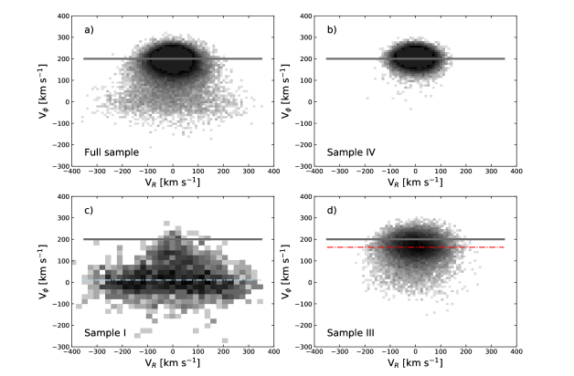
We start by studying our stellar samples defined in the Mg-Mn-Al-Fe-plane in various kinematic spaces. Figure 5 shows as a function of for the full sample and for Sample I, III, and IV as defined in Fig. 2. In each panel the median value for of the full sample is shown as a grey line, whilst the median of the selected sample is shown as a coloured, dashed line. For Sample IV the grey and the coloured lines have the same value. Sample I shows an elongated structure centred at and an extension of stars to higher (pro-grade) -values which is centred at . Sample IV is, as already noted, very similar to the bulk of the full sample, whilst Sample III has a distinctly lower mean -value as well as an extension towards and even negative values (retro-grade).
To summarize, the main sample is well concentrated around (, ) = (0, ) km s-1. When divided into sub-samples using the Mg-Mn-Al-Fe-plane we find that one sample takes up the bulk of the stars centred at the same values as the main sample whilst the other two samples contain the stars making up the down-ward flow of stars towards as well as flaring out to larger (pos/neg) values of . The three samples are distinct in the (, )-plane.
Recently, another depiction of the stellar kinematics has been used – the action diamond (Vasiliev, 2019; Myeong et al., 2019; Lane et al., 2022). The diamond is constructed from the actions and angular momenta of the stellar orbits. On the -axis is and on the -axis . As explained in Lane et al. (2022) this space is particularly intuitive to interpret; the left- and right-hand corners occur when the angular momentum in the -direction and the total action are equal, i.e. a pro- or retro-grade orbit in the plane. The bottom corner contains the stars on purely radial orbits while the top corner gathers the stars on polar orbits.
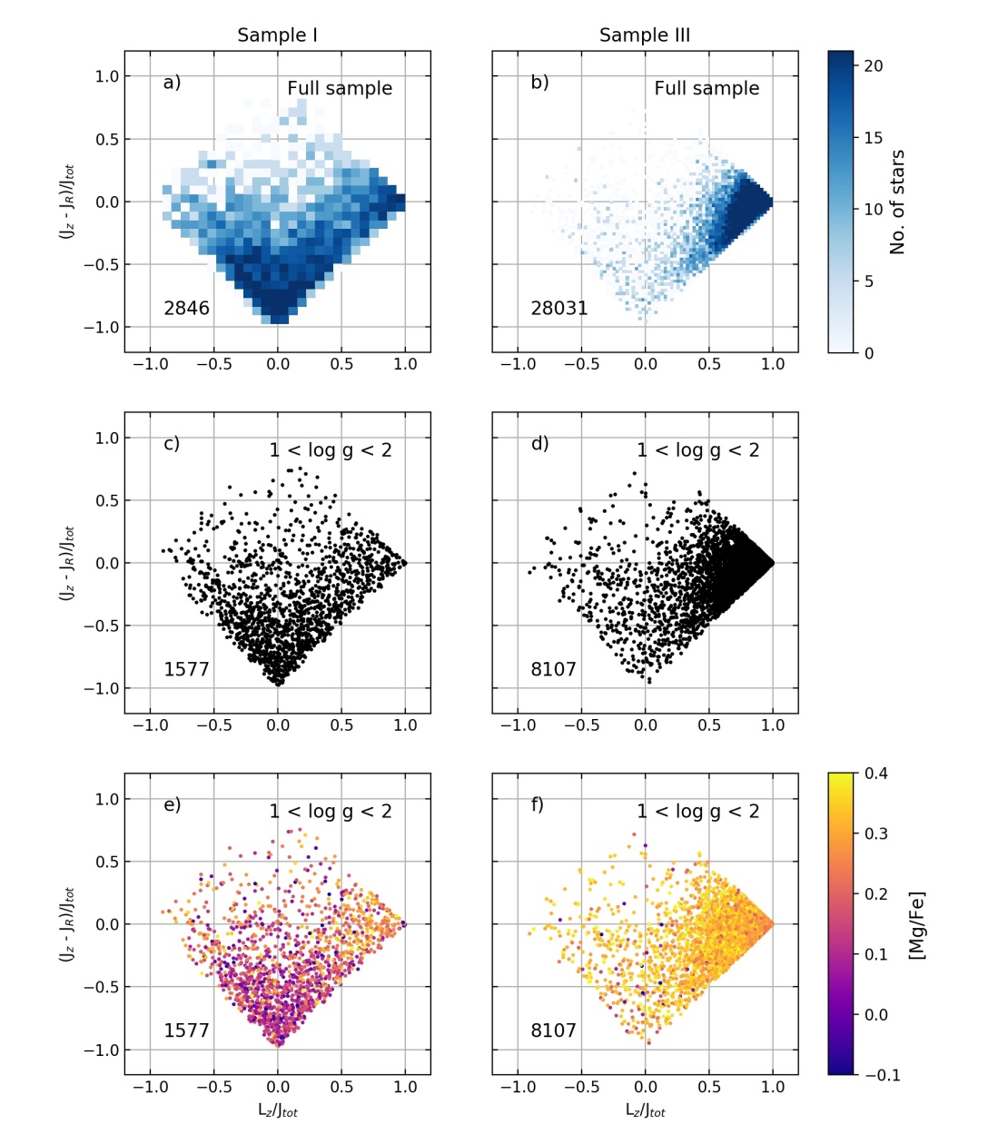
Figure 6 a) and c) show the action diamonds of Sample I for the full sample and for only stars with , respectively. In both cases, the sample is mainly concentrated to the bottom corner. The bottom corner of the action diamond is associated with radial orbits (see Sect. 4.1.1 in Lane et al., 2022). However, the figures also show that there is a smaller concentration of stars in the right hand corner. This corner is associated with pro-grade disk-like orbits. Figure 6 b) and d), show the action diamonds of Sample III for the full sample and for only stars with , respectively. Sample III populates the right-hand corner of the action diamond associated with disk-like orbits (Lane et al., 2022). Fig. 6 e) and f) show the action diamonds of Sample I and III for stars with , colour-coded according to the [Mg/Fe]-ratios of the stars. Sample I shows mainly low(er) [Mg/Fe]-ratio than Sample III. However, the stars in the left- and right-hand corners of the action diamond for Sample I have high-[Mg/Fe] ratios suggesting there may be two stellar populations in Sample I.
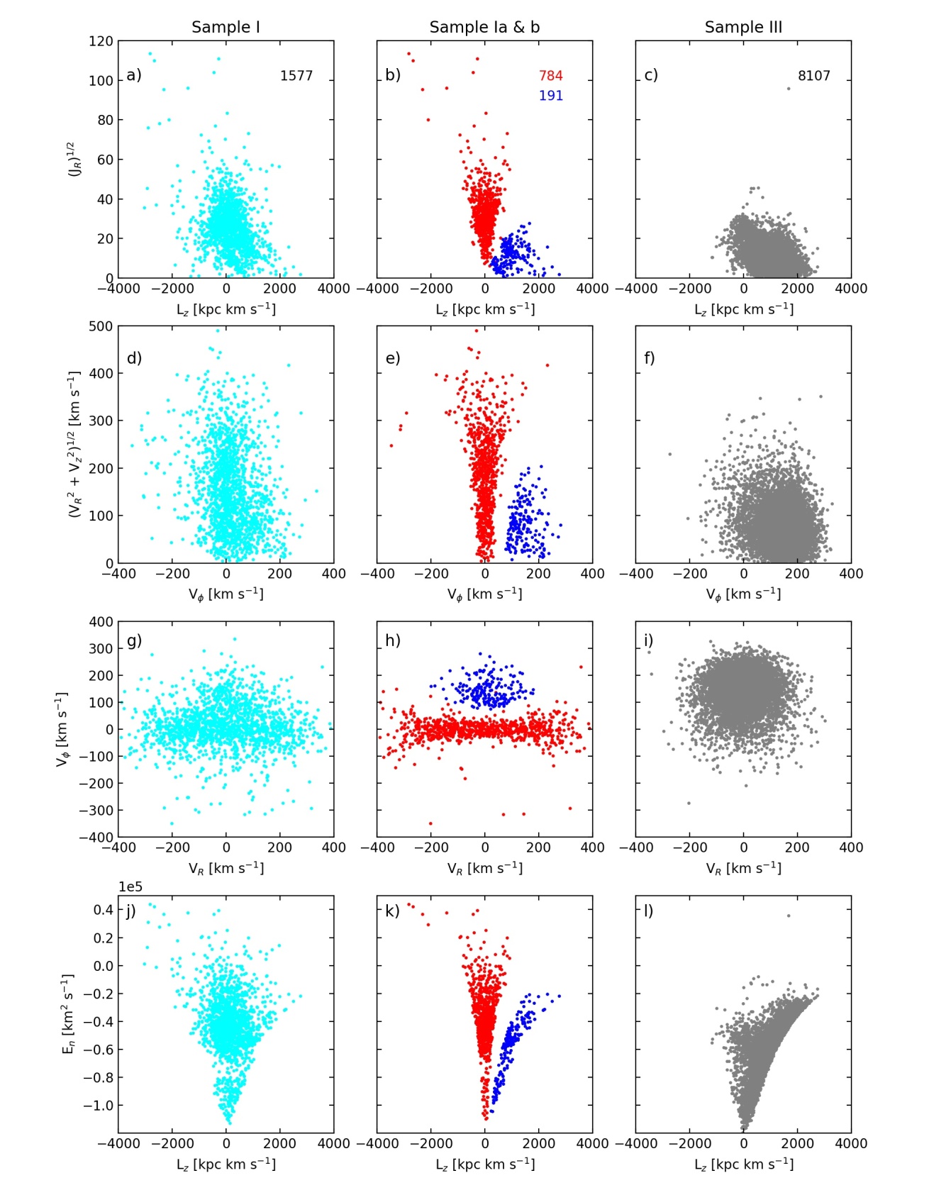
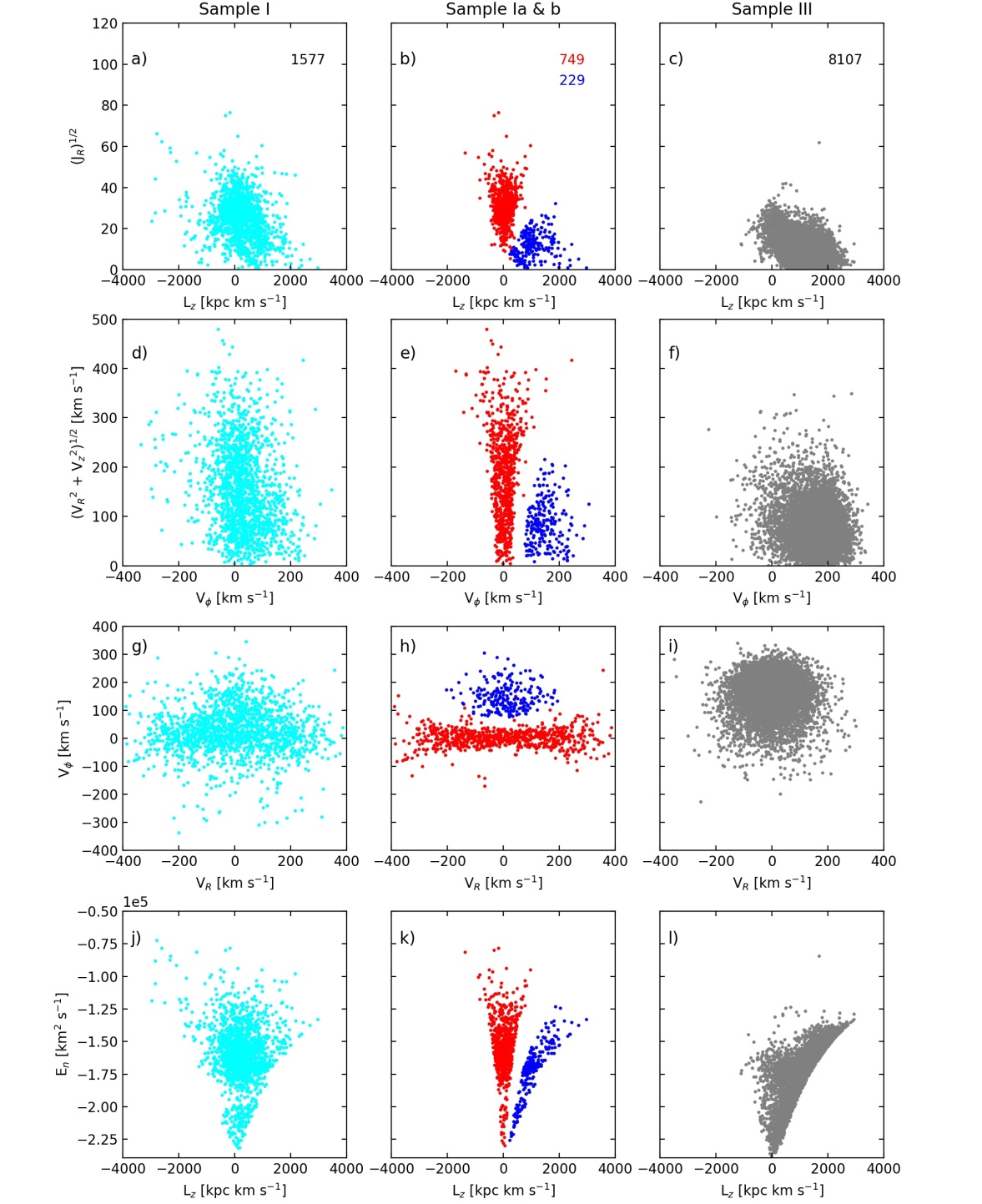
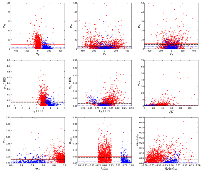
To ensure that our interpretation of the properties of Sample I as seen in the action diamond actually implicates two stellar populations with different kinematical status we show four commonly used kinematic planes. We define two sub-samples in Sample I based on the stars’ . Sample Ia is defined as stars with and Sample Ib stars with . Figure 7 shows the four kinematic spaces for the two new Sample Ia (red) and Ib (blue), as well as Sample I and III. For all samples, only stars with are shown444We note that for the orbital calculations with galpy we have used the MWPotential2014 in Bovy & Rix (2013); Bovy (2015). To be compatible with other studies we also present the same plots using the McMillan (2017) potential in Appendix B. The conclusions remain, the main difference being the values of , which are shifted..
We observe that the kinematical properties of Sample I and III are distinct. Remember that these selections are only based on elemental abundances (Fig 2). Sample I has mainly radial orbits of the type associated with the halo and Sample III can best be described as a somewhat heated disk, with most stars on prograde orbits. Sample Ia and Ib indeed show the expected dichotomy – Sample Ia has a radial orbit (as per design) while Sample Ib clearly is picking up essentially all the disk-like stars in Sample I. Note that there will be a gap between the samples as per the selection.
To summarise, Sample I contains two stellar samples identified in the action diamond, one on radial orbits and one on disk-like pro-grade orbits. Sample III contains an essentially disk, pro-grade stellar sample.
5.2 Chemical properties of Sample I and Sample III
We now turn to the chemical properties of Sample I, Ia, Ib, and III. We start by noting that Fig. 6 e) and f) show that Sample I and Sample III have distinct chemical properties where Sample III contains almost exclusively stars with [Mg/Fe] 0.25. In Sample I, stars with [Mg/Fe] 0.2 are mainly concentrated towards the bottom corner of the action diamond. The right- and left-hand corners are dominated by stars with [Mg/Fe] 0.25 There are also some stars spread into the rest of the action diamond with high [Mg/Fe]-ratios.
To summarise, it appears that the two kinematical sub-samples in Sample I identified in Sect. 5.1 have distinct chemical signatures with the stars on disk-like orbits being elevated in [Mg/Fe] in comparison to the stars with radial, halo-like orbits.
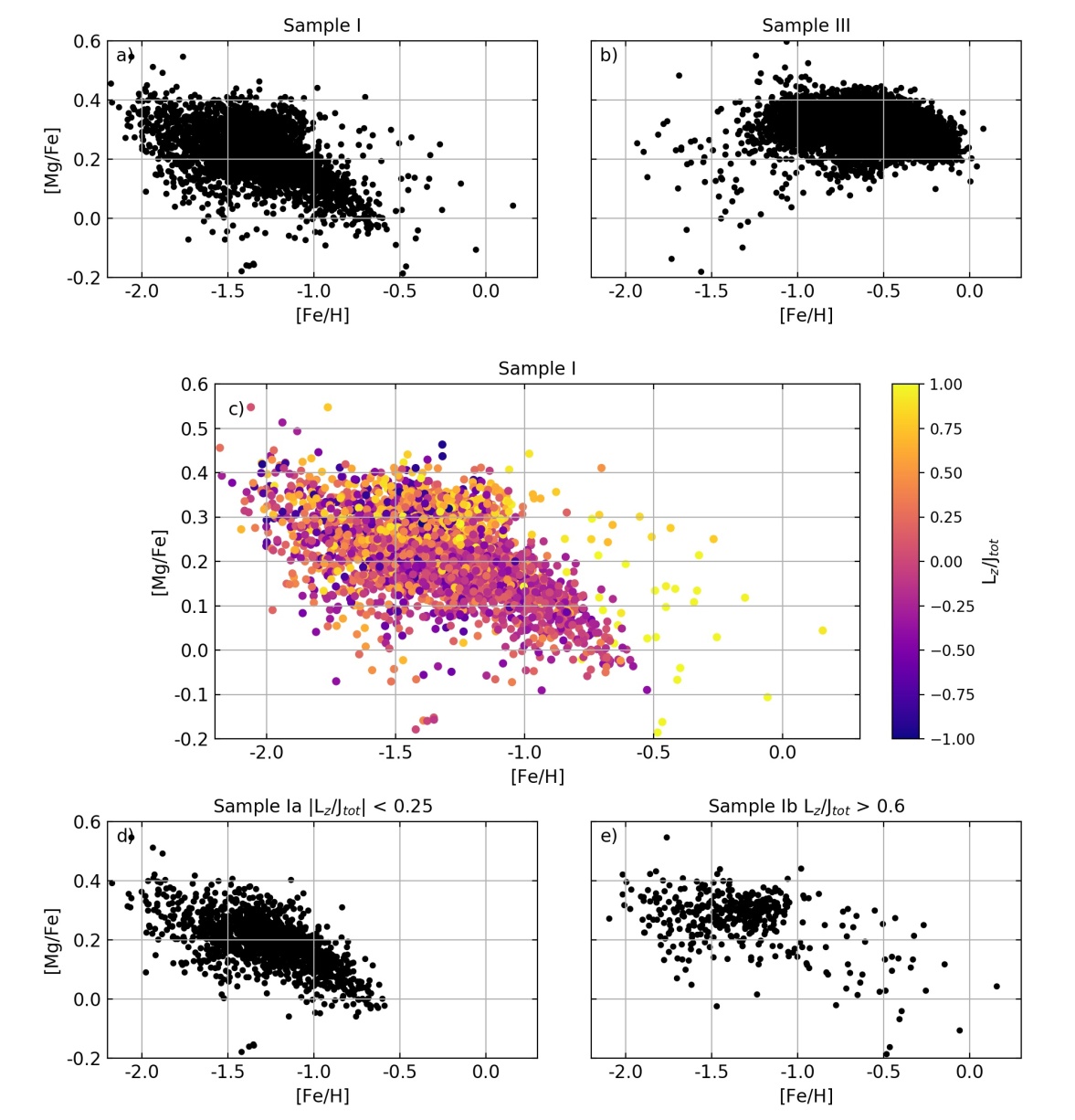
Fig.ure 8 a) and b) show [Mg/Fe] as a function of [Fe/H] for Sample I and III. These are clearly distinct with Sample III being more metal-rich (median [Fe/H] = –0.55) and showing high [Mg/Fe] for all stars. Sample I has lower [Fe/H] (median [Fe/H] = –1.33) and a downward trend for [Mg/Fe], starting from the highest values and continuing down to about 0.0 dex.
Figure 8c) shows the stars in Sample I colour-coded according to . Here we find that almost all stars with positive have high [Mg/Fe]-ratios, while stars with around zero follow the down-ward trend. To more easily see this, Fig. 8 d) and e) show Sample Ia and Ib, i.e. and , respectively. Sample Ib has a high [Mg/Fe]-ratio with only a sprinkle of stars with lower ratios. The sample also stops quite abruptly at [Fe/H] about –1.1 dex. We note that Sample III starts roughly at the same iron abundance as Sample Ib stops, suggesting Sample III could be a later stage evolution of Sample Ib. Figure 19 shows that [Ni/Fe] behaves in the same way as [Mg/Fe]. In fact, the picture is even a bit clearer when using [Ni/Fe].
5.3 Potential selection effects
With large spectroscopic surveys, inevitably the selection function of the survey may influence the perceived properties of a stellar population (Mints & Hekker, 2019; Stonkutė et al., 2016). Preferably it should be possible to correct for the introduced biases or model their effect on the data in order to capture the underlying truth. This, however, can be more or less difficult to do and the examples in the literature are few. In the present work we are foremost concerned with identifying and characterising stellar components with the help of elemental abundance trends. The interpretation of such data does not need a complete sample but it is important to understand if certain parts of the Galaxy or parameter space have been excluded thanks to the selection function of the original survey or via a too vigorous down selection of objects in the study itself.
To ensure that our conclusions are robust we have looked at the spatial properties of our samples and also at what effects the original APOGEE selection function may have on the phase space data we are using.
Spatial properties of our samples
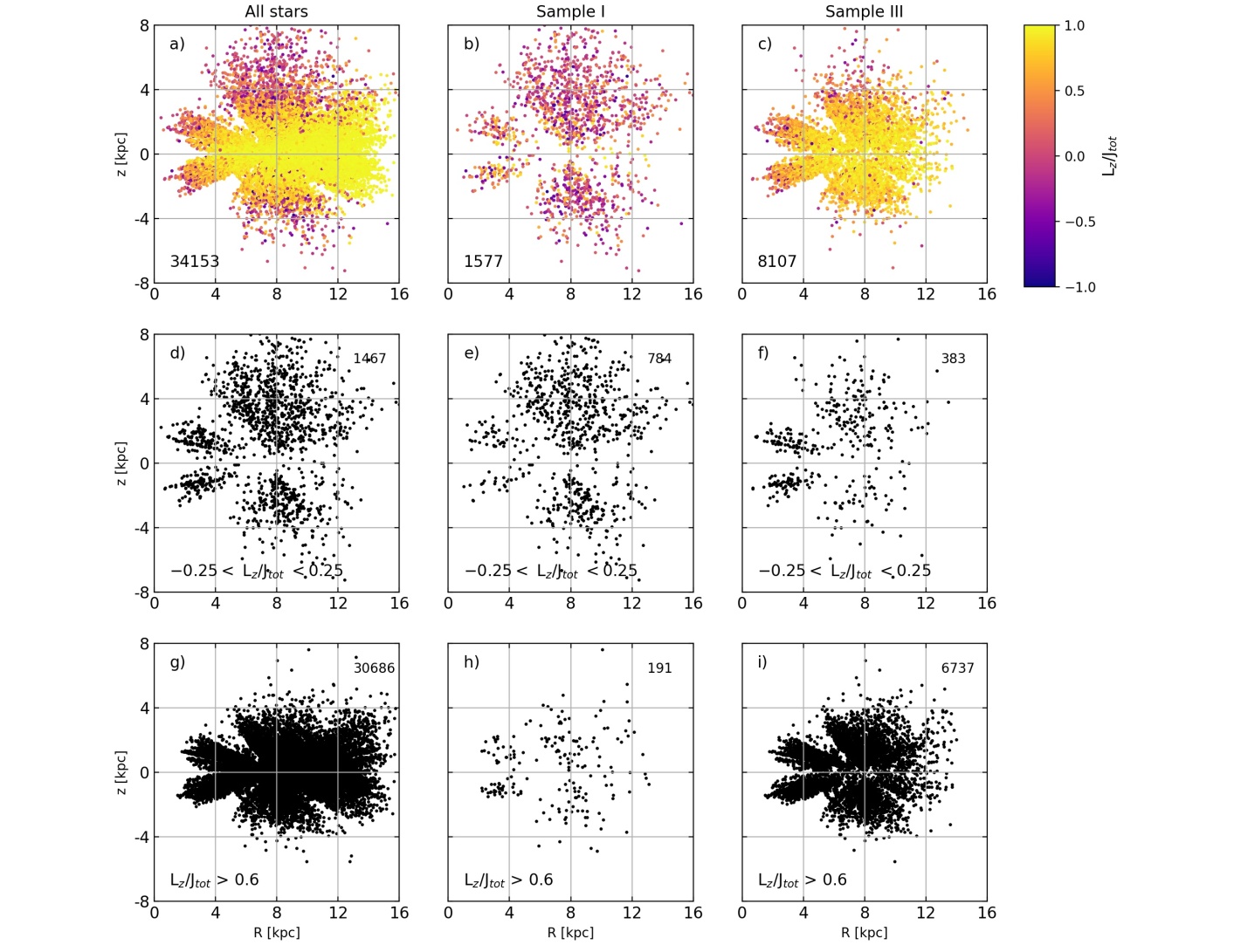
The top-row of Fig. 9 shows the --plane for our full sample, Sample I and III, colour-coded by . Visual inspection shows that Sample I covers the full extent in of the full sample, that it also covers a fair portion of the , but that there is a lack of stars with these chemical signatures in the disk beyond the solar position (Fig. 9 b). Sample III is more confined to the plane ( kpc, Fig. 9c) and covers the disk better than Sample I.
Rows two and three further divide the data into (i.e. halo-like orbits) and (i.e. disk-like orbits). In all three cases this division shows that stars with halo-like orbits occupy the full space spanned by all stars (potentially with some lack of stars outside the solar orbit in the plane) and stars with disk-like orbits are more confined to the plane.
As we observe the same behavior for the full sample and for Sample I and III, we conclude that there is no direct indication that our results should not be valid for the whole Galaxy, i.e. the properties of the stellar populations we observe are not just a local, but a global phenomenon.
Selection effects showing up in the plane
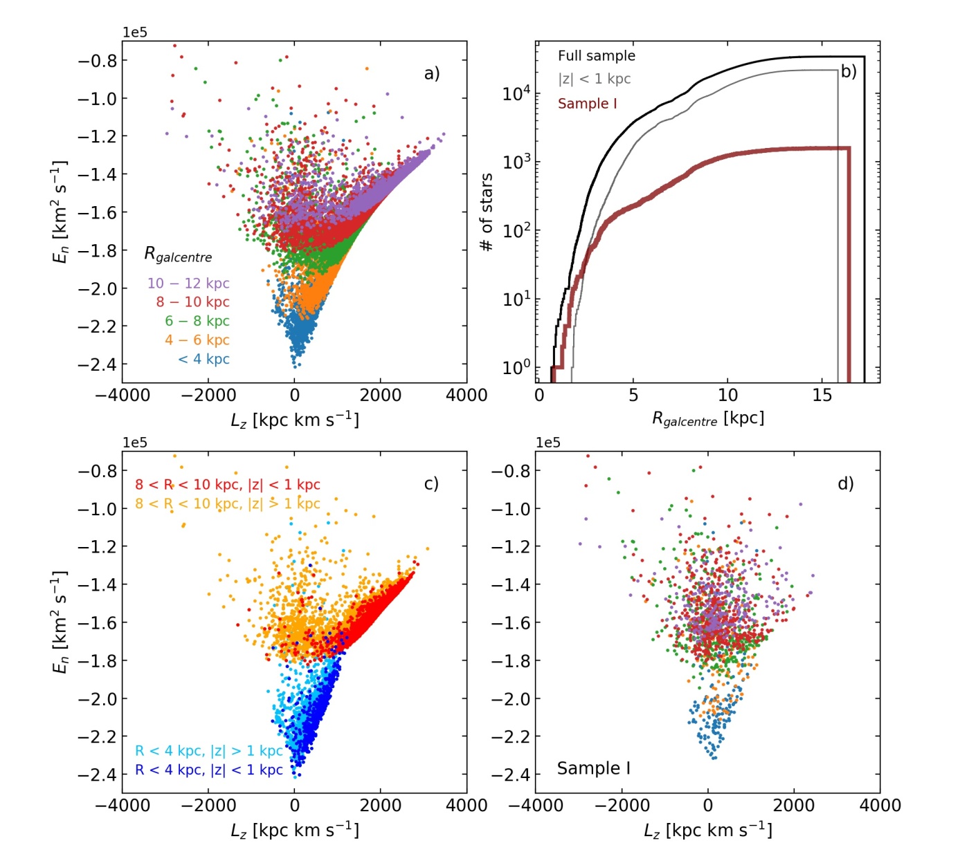
Figures 9 and 10 highlights an underlying selection effect from the original APOGEE DR17 sample. In Fig. 10 a) our sample stars are shown colour-coded according to their galactocentric distances. Stars in the plane at a given distance in a galactic potential follow a certain parabola in the plane (see Fig. 5 in Lane et al., 2022). As expected, stars at a certain radius follow a parabola. The upward scatter in each sample is due to the sampling of stars at different heights above the Galactic plane. This is illustrated in panel c) for two radial bins ( and kpc) where stars with kpc are shown in a fainter colour. At a given these stars are more spread in than stars at lower .
In Fig. 10 d) we show the data for our Sample I. Remember that this sample is simply selected based on the elemental abundances of the stars (Table 2). The plane shows a clear lack of stars for to . Is this gap real or part of a selection effect? In panels a) and d) of Fig. 10 we have colour coded the stars according to their galactocentric distances. We can see that the energies for the gap corresponds to radial distances of about 5 kpc. As discussed in Lane et al. (2022) the observing strategy of APOGEE (for DR16 but also for DR17) includes some extra deep fields towards the Galactic bulge. These result in an excess of stars observed closer to the Galactic center, at a lower than the nominal disk survey (their Fig. 6) If we refer to Fig. 9, we can see that the galactocentric distance of 5 kpc is less populated than other radii thanks to the placement of the two deep pointings at low latitude while the main survey observed at high latitudes reaching well above the Galactic plane. This survey strategy has left a clear gap in stellar distribution seen edge-on. This gap is present in all our samples and is thus not a feature of the selection in the Mg-Mn-Al-Fe-plane.
We can thus assume that our results are not biased, however, we are missing objects around 5 kpc (compare Fig. 10 b). There is no reason to assume these objects do not exist but will be found in future surveys.
6 Dating the stellar components
It would be interesting to date the Sample Ia and Ib to further understand their role in the formation of the Milky Way. We are using RGB stars for our studies and hence it is not feasible to obtain good ages for individual stars using isochrone fitting (Soderblom, 2010; Sahlholdt et al., 2019b). However, asteroseismology offers an alternative possibility to derive ages for RGB stars (see e.g. Miglio et al., 2017, 2021). We searched the literature for ages derived from asteroseismological observations for stars with similar characteristics to those we find in Sample I and found two studies: Montalbán et al. (2021) and Borre et al. (2022). Although these are relatively small studies they can still give us some first hints as to the nature of the ages of our samples and also point to which specific studies would help to better constrain our observations.
We first took a look at the overlap between the two datasets and how many of the stars in the two studies would fall into our Sample I. We found that the overlap is, for the objective of our study and focus on Sample I, sufficiently large that nothing is gained by using both samples and we thus selected Borre et al. (2022) as being the sample with more stars falling in Sample I.
6.1 Data
Borre et al. (2022) studied a sample compiled from a cross-match between asteroseismic data from the Kepler mission, astrometric data from the Gaia mission, elemental abundances from APOGEE DR16, and the Two Micron All Sky Survey (2MASS). For references and details of the selection of stellar data, final target assembly, and calculation of stellar ages and space motions we refer the reader to Sect. 2 in Borre et al. (2022).
In total, Borre et al. (2022) provide ages for 70 stars based on photometric, asterometric, and asteroseismic data (individual frequencies or and ). Here we are interested in the ages provided by this study and less with their target selection. However, it is worth noting that they start from a kinematic selection (defined in ). This results in a large range of [Fe/H] values.
Borre et al. (2022) used elemental abundances from APOGEE 16 (Ahumada et al., 2020). In our work we are using APOGEE DR17 (Abdurro’uf et al., 2022). The exact values of [Fe/H] as well as [/Fe] will to some extent influence the derived stellar ages. Figure 10 in Borre et al. (2022) provide a comparison of [Fe/H] values used in their study and in Montalbán et al. (2021), who use APOGEE DR14, showing offsets ranging from 0 to about 0.2 dex. In the same figure there is also a comparison of the ages derived for the stars which shows the ages to have small differences (from 0 to about 2 Gyr). In all cases, the ages derived in the two studies agree well within the error bars. We conclude that the small offsets in [Fe/H] between APOGEE DR16 used to derived the ages and APOGEE DR17 used in our elemental abundance selection are negligible, and that the choice of Borre et al. (2022) ages over Montalbán et al. (2021) will not influence our conclusions.
The elemental abundances for this sample are shown in Fig.11.
6.2 Age of the stars in Sample I
| Gaia ID | [Fe/H] | [Mg/Fe] | Age | Age error | Ia | |
|---|---|---|---|---|---|---|
| 53635139275591040 | –1.38 | 0.20 | 11.69 | +2.57/–2.82 | +0.038 | ✓ |
| 2099659187162016512 | –1.37 | 0.34 | 11.75 | +1.91/–1.20 | –0.113 | ✓ |
| 2126445115779806976 | –1.43 | 0.24 | 5.54 | +1.88/–3.18 | –0.252 | – |
| 2127447522484965504 | –1.50 | 0.36 | 10.51 | +2.18/–1.82 | –0.480 | – |
| 2133314619611880448 | –1.56 | 0.27 | 10.27 | +1.96/–2.50 | +0.092 | ✓ |
| 2538202737087917184 | –0.87 | 0.13 | 9.85 | +3.40/–3.45 | +0.170 | ✓ |
| 2626567188077168896 | –0.77 | 0.09 | 4.59 | +4.23/–2.19 | –0.026 | ✓ |
In Table 3, we list those stars that fulfill our quality criteria and fall in Sample I (see Table 1 and 2). We note that our quality criteria are more restrictive than those applied in Borre et al. (2022), this is likely partly due to different versions of APOGEE being used. We also consider those stars that would be selected based on their elemental abundances if we disregarded the quality flags we applied.
We find an average of Gyr for the 7 stars that fall in the Sample I region in the Mg-Mn-Al-Fe-plane and fulfill our quality cuts. Two of the stars have young ages, typical of the stellar disk. If those are excluded the age is Gyr. If we use our cut in to consider the stars in Sample Ia (see Sect. 5.1), we are left with five stars that have a mean age of Gyr. If the young star is excluded we obtain a mean age of Gyr.
We can conclude that the stars that fall in Sample I or Sample Ia and fulfill our quality criteria for the elemental abundances have an old age. There are two stars that have young ages. Such stars have been found also in other studies and are sometimes referred to as young -rich stars (Chiappini et al., 2015). One explanation for the presence of such stars is that they are in fact blue stragglers (Jofré et al., 2016).
None of the stars in the seismic sample that fall in the Sample I region in the Mg-Mn-Al-Fe-plane have , i.e. stars in Sample Ib. This means that although we can put an age on Sample Ia we are unable from the presently available stellar ages to derive an age for Sample Ib, i.e. the disk.
7 Discussion
| Panel | Study | Selection ctriteria | Units | ||||
|---|---|---|---|---|---|---|---|
| i) | “Sausage” | km s-1 | |||||
| f) | Helmi et al. (2018) | kpc km s-1 | |||||
| km2 s-1 | |||||||
| c) | Myeong et al. (2019) | ||||||
| h) | Feuillet et al. (2020) | 30 | (kpc km s-1)1/2 | ||||
| 500 | kpc km s-1 | ||||||
| b) | Horta et al. (2022) | kpc km s-1 | |||||
| km2 s-1 | |||||||
| e) | Naidu et al. (2022) | km2 s-1 | |||||
| 0.7 | |||||||
| 5 | kpc | ||||||
| [Mg/Mn] | |||||||
| [Mg/Mn] [Al/Fe] | |||||||
Following the work by Hawkins et al. (2015) and Das et al. (2020) we have explored the ability of the Mg-Mn-Al-Fe-plane to distinguish stars from different stellar populations in the Milky Way. By further combining the elemental abundance data with kinematical properties of the stars we have found that the region with low [Al/Fe]-values (our Sample I) contains stellar populations with kinematical properties associated with the stellar halo and with the stellar disk. Furthermore, we find that those samples differ in their [Mg/Fe] and [Ni/Fe] abundance trends, indicating different origins.
7.1 Gaia-Sausage-Enceladus
When the astrometric data from the ESA Gaia satellite are combined with radial velocities it is possible to study the halo kinematics in great detail. Using different techniques, research teams have found stellar populations, accreted galaxies, and stellar streams.
The Gaia-Sausage-Enceladus and other discreet stellar populations have been found thanks to the astrometric data from the ESA Gaia satellite (Helmi et al., 2018; Belokurov et al., 2018; Helmi, 2020; Naidu et al., 2022; Horta et al., 2022).
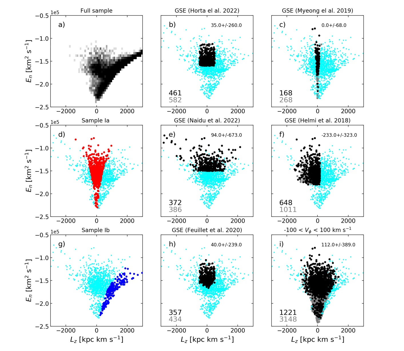
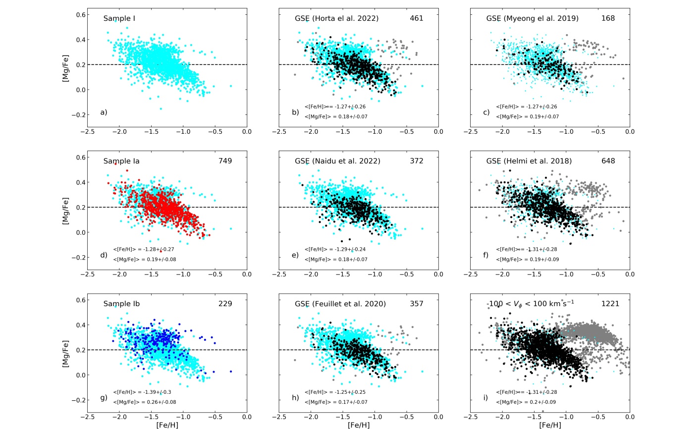
In Table 4 we have, from the literature, collected five different ways of selecting Gaia-Sausage-Enceladus stars. We also include a kind of trivial definition of the Sausage, i.e. km s-1. Figure 12 a) shows a 2D histogram of the plane for our full sample. In all remaining panels, our Sample I is shown in cyan for comparison. Our Sample Ia and Ib are shown in panels d) and g). In the other panels we show the resulting distributions in the plane when we select stars from our main sample according to the six Gaia-Sausage-Enceladus criteria listed in Table 4. We show two selections for each sample. Grey points indicate stars selected from our catalogue only using the criterium listed in Table 4 and the number of selected stars indicated in grey in the lower left-hand corner of each panel. Black points indicate stars that also fall into our Sample I (Table 2) and the number of such stars is indicated in black in the lower left-hand corner of each panel. In the upper right-hand corner of the six Gaia-Sausage-Enceladus panels, the average and associated are shown.
It is interesting to note that the five definitions of Gaia-Sausage-Enceladus taken from the literature show distinctly different distributions in the plane. In all cases, imposing our selection criterium in the Mg-Mn-Al-Fe plane lowers the number of stars but it does not seem to change the distribution in the plane much apart from for the trivial definition shown in panel i), where we can see that the gap is less prominent in the grey points than in the black ones. A similar effect is suggested in panel c) using the criterium from Myeong et al. (2019).
It is immediately obvious that our Sample Ib bears little resemblance in the plane to any of the definitions of the Gaia-Sausage-Enceladus. This is not surprising given that we find it has disk-like kinematics. Our Sample Ia on the other hand occupies many of the same spaces in as the six definitions. The distribution based on selection by Myeong et al. (2019) is the one most similar to our Sample Ia. In general though the literature definitions avoid the lower energies included in Sample Ia. These are only present in the trivial definition and in Myeong et al. (2019). Feuillet et al. (2020) and Horta et al. (2022) have quite similar distributions while Naidu et al. (2022) has a much wider distribution in than the other two. It also reaches higher energies. Finally, we note that the selection criteria defined by Helmi et al. (2018) creates an essential retrograde population, which reaches to quite low energies.
Fig. 13 presents the associated distribution of [Mg/Fe] as a function of [Fe/H] for Sample I, Ia, Ib, and all six definitions of Gaia-Sausage-Enceladus. Colour-coding is the same as in Fig. 12, but here we only print the number of stars fulfilling both the literature criteria and our selection in Mg-Mn-Al-Fe-plane. In addition, each panel shows the average [Fe/H] and [Mg/Fe] for the black points.
There are three immediate observations to be made from these plots: 1) Regardless of selection criteria all selections result in a down-going trend for [Mg/Fe] with increasing [Fe/H]. The trend coincides with our Sample I and even more clearly with Sample Ia. 2) In all cases adding our selection in the Mg-Mn-Al-Fe-plane removes the high [Mg/Fe] stars at higher [Fe/H], i.e. the disk. 3) In all but the trivial case there are stars more enhanced in [Mg/Fe] at a given [Fe/H] in Sample I (cyan). These stars are deselected in all but the trivial case and overlap with our Sample Ib in this plane.
Various investigations have used kinematic criteria and/or various clustering algorithms to identify groups of stars that likely come from a single accreted progenitor. We find that the Mg-Mn-Al-Fe-plane is suitable for identifying stars with halo kinematics and likely accreted origin, but we find that the same region also includes stars with typical disk kinematics. When we study the elemental abundance trends, we find that, regardless of selection method, samples that can be associated with the Gaia-Sausage-Enceladus progenitor show remarkably similar elemental abundance trends but not always the same kinematic characteristics. In particular, the accreted stars appear to be able to have both pro- and retro-grade orbits. It appears remarkable that regardless of criterium used, we recreate the same downward [Mg/Fe] trend first observed by Nissen & Schuster (1997, 2010). Thus it appears that the stars from this merger are well-mixed in kinematics but better distinguished in elemental abundance space.
The Hestia simulations (Libeskind et al., 2020; Khoperskov et al., 2022a, b, c) follow three Local Group pairings of galaxies and their respective merger histories. One important aspect of these simulations is that the galactic potential evolves in the cosmological context. This means that after a smaller galaxy merges with the main progenitor the potential gets deeper with time. The effect is that, regardless of time of merger, all of the major mergers have roughly the same energy today. This means that the – plane is partly degenerate when it comes to picking up individual merger debris. Another important information gleaned from the inspection of the – diagrams for the mergers in the Hestia simulations is the fact that almost all mergers show stars on both pro- and retro-grade orbits. This is very similar to what we find when we are looking at the stars that, in various ways, could be associated with the Gaia-Sausage-Enceladus.
Massari et al. (2019) studied the globular cluster system in the Milky Way and defined the Main Progenitor as the properties traced by globular clusters formed in situ in the stellar disk or the Galactic Bulge. The left panel of Fig. 2 in Massari et al. (2019) shows the – plane of Milky Way globular clusters. It is interesting to note that the clusters associated with the Main Progenitor have a distribution in the – plane that is strongly reminiscent of our Sample Ib. Kruijssen et al. (2019), in a similar manner, used globular clusters to trace early merger events in the Milky Way and identified what they claim to be one such event; the deeply bound Kraken galaxy. We have tentatively looked at the deeply bound portions of our samples, compare also the trivial definition of the Gaia-Sausage-Enceladus presented earlier. We find some similarities in elemental abundance space with our Sample Ib and a Kraken sample.
A recent critique of the practice of using the globular clusters to trace the formation and assembly history of a galaxy can be found in Pagnini et al. (2023). They study the accretion of galaxies and associated globular clusters onto a galaxy where the potential is allowed to change as the main galaxy grows via mergers over cosmic time. In agreement with the main findings of the Hestia simulations, they show that the globular clusters from the merged galaxy do not end up in the same part of the – plane as stars from their host galaxy. Only for small galaxies may there remain some similarities in kinematic properties between the field stars accreted from the smaller galaxy and its globular clusters.
7.2 The chemically unevolved stellar disk
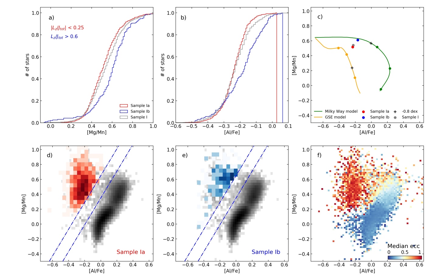
Earlier (Sect.5.1) we found evidence that Sample Ib is part of the disk of the Milky Way and not the halo even though the stars fall in the region of the Mg-Mn-Al-Fe-plane thought to (mainly) harbour halo and/or accreted stars. Figure 14 a) and b) shows the cumulative distributions of [Mn/Mg] and [Al/Fe], respectively, for Sample I, Ia and Ib. It is immediately clear that the kinematically defined sub-samples differ. Sample Ib is more enhanced in both [Mg/Mn] and [A/Fe]. In Fig. 14 c) we compare the median values of the elemental abundances for our three samples with the two chemical evolution models by Horta et al. (2022). Sample Ib lies close to the evolutionary track of the Milky Way model, while the full sample as well as Sample Ia tend more towards the GSE model thus giving further support to our interpretation that Sample Ib really is the (chemical) beginning of the Milky Way disk.
In Fig. 14 d) and e) we look at the distributions of the data for Sample Ia and Ib in the Mg-Mn-Al-Fe-plane using a 2D histogram. We find that not only do their median values differ, but also the distribution of the stars in this plane. Sample Ia shows an elongated, more or less vertical distribution, while Sample Ib shows a horizontal distribution and is a more chemically enriched population. The two kinematically defined sub-samples in Sample I clearly occupy two chemically distinct populations – one seemingly following a trajectory that could describe an accreted dwarf galaxy and the other a trajectory that would connect well to the chemical evolution of the main body of the Milky Way when compared with chemical evolution models.
Finally, we look at some of the kinematic information for our whole sample in Fig. 14 where we show all stars in the Mg-Mn-Al-Fe-Plane binned into a 2D histogram where the colour represents the median eccentricity of the stars in each bin. There are several things to note from this plot. The first one is that the distribution of eccentricity changes between different regions of the plane.
In particular, stars that fall virtually in the same place as Sample Ia have a mean eccentricity of 0.90 (with a =0.10 and median eccentricity uncertainty of 0.03), i.e. radial orbits. Stars in the region occupied by Sample Ib show a lower mean eccentricity of 0.37 (with a =0.16 and median eccentricity uncertainty of 0.01). This carries over into the region where Sample III sits with mean a eccentricity of 0.38 (with a =0.21 and a median eccentricity uncertainty ) and then flows down towards lower [Mg/Mn], decreasing in eccentricity such that Sample IV is almost entirely on circular orbits with a mean eccentricity of 0.15 (with a =0.09).
This figure is a nice illustration that the stars on eccentric orbits, i.e. accreted stars, are found in a particular region of the Mg-Mn-Al-Fe-plane, but that they do not occupy the whole area that is normally assigned to the accreted region. Instead only a specific region is occupied. This shows that although we originally divided our Sample I into two extremes, as concerns their kinematics, we still picked up the major accreted component – presumably the Gaia-Sausage-Enceladus. The stars with disk kinematics in Sample I on the other hand connect kinematically quite well to Sample III which harbours the stars we ordinarily associate with the thick disk, and possibly with the Splash to some extent.
We summarise that the stellar disk extends into the regions in the Mg-Mn-Al-Fe-plane associated with merger debris. The kinematics of the whole plane shows that this part of the stellar disk, the chemically unevolved disk, smoothly connects to the hotter part of the disk that is also significantly chemically enriched.
7.3 Estimating the accreted fraction of stars

If we want to understand how galaxies form and evolve we would like to know how much of the stellar mass has formed in the galaxy itself and how much has been accreted. If stars formed in smaller galaxies have elemental abundance signatures that make them stand out from those stars that have formed in the galaxy itself that would be one way of estimating how many of the stars in a galaxy today have actually formed in other galaxies and this would then give us constraints on galaxy formation in general.
As we have discussed, the Mg-Mn-Al-Fe-plane is a good place to identify stars formed in other galaxies. But, we have also shown that the area associated with the signatures of smaller stellar systems in the Mg-Mn-Al-Fe-plane also contains stars belonging to the (old) disk. This is not unexpected given the modeling results by Horta et al. (2022). However, we think it is still of interest to obtain an upper limit to the number of accreted stars in our sample as well as obtaining maps that show us where the majority of accreted and in situ stars are situated.
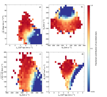
Here we use Sample I in its entirety to represent accreted stars. This thus gives us an over estimate of the fraction of accreted stars as Sample I includes stars on disk orbits. The accreted fraction of stars with a kinematic signature is simply the number of stars in Sample I divided by the total number of stars. Fig. 15 shows our results in four kinematic spaces. In these plots pixels with two or fewer stars have been removed. Figure 16 shows the same type of data but now presented in the action diamond.
We see that the kinematic region associated with the Gaia-Sausage-Enceladus shows up as dark blue regions in all four spaces in Fig. 15 (compare e.g. Feuillet et al., 2021, and Fig. 12) but the action diamond appears to be a lot less sensitive to pick out the accreted stars (see Fig. 16). In Fig. 15 d) we see that for low energies, i.e. tightly bound orbits below km2 s-1, the fraction of accreted stars is about 10–30% for stars on orbits with close to zero. This is interesting as it is indicating that based on the stellar chemical make-up we are seeing stars that have formed in the main galaxy here, i.e. there is not just accreted stars but we are seeing evidence for the main progenitor.
Thus, even though the central parts of the Milky Way may harbor accreted components there is a substantial portion of in situ formed stars that should belong to the initial galaxy. This would agree with our finding that Sample Ib is a disk-like population.
8 Conclusions
We have for the first time identified the early stellar disk in the Milky Way by using a combination of elemental abundances and kinematics.
Stars accreted on to the Milky Way by other (smaller) galaxies merging with our Galaxy can be difficult to find. In particular kinematic signatures may be erasade more quickly and completely than previously though when the evolving Galactic potential is taken into account. Instead, we turn our attention initially to the elemental abundances in the stars.
Hawkins et al. (2015) and Das et al. (2020) empirically found that the elemental abundance plane spanned by [Mg/Mn] and [Al/Fe] could be used to identify accreted stars. Horta et al. (2021) further discussed this possibility underpinning their arguments with chemical evolution models. We re-address the validity of the Mg-Mn-Al-Fe-plane for identifying accreted debris and find that it is useful also when taking issues related to the derivation of elemental abundance, such as departures from LTE, into account. As illustrated in Fig. 3, the selection of clumps of stars in the Mg-Mn-Al-Fe plane is robust against departures from NLTE and 3D for the red giant branch stars used in this study.
We proceed to use this abundance plane to identify the accreted/halo component solely using elemental abundances, which we refer to as Sample I. The kinematical properties of the stars in Sample I contains, as expected, stars with all the kinematic hallmarks of being accreted, but we also find stars on clear disk-like orbits. We also find that the spatial distribution of the stars differ. Stars with disk-like kinematics are (more) confined to the Galactic plane.
We further analyse the properties of the two sub-samples and identify the accreted stars (mainly) with the Gaia-Sausage-Enceladus whilst the disk stars are the start of the main body of the Milky Way disk (as predicted by chemical evolution models). The stars in Sample I with disk-like orbits have higher [Mg/Fe] as a given [Fe/H] than the stars in Sample I with halo-like orbits, see Fig. 8, similar to a thick disk population.
We have thus for the first time identified the early stellar disk by using a combination of elemental abundances and kinematics.
In addition, we show that the selection of Gaia-Sausage-Enceladus in the -plane is not very robust. This is in line with recent numerical simluations which indicate that merger signatures are erased also in this plane (Khoperskov et al., 2022b; Pagnini et al., 2023).
Our study shows the need to carefully combine both elemental abundances and kinematics to make progress understanding the mass accretion and early history of the Milky Way. The latest Gaia data release, as well as the new and upcoming massive spectroscopic surveys (WEAVE, GALAH, APOGEE, SDSS-V, DESI, LAMOST, 4MOST), will provide the necessary data.
Appendix A Additional information on the selection of stars from APOGEE DR17
A.1 APOGEE fields and programs excluded
47TUC |
ANDR* |
BOOTES1 |
Berkeley* |
CARINA |
COL261 |
CygnusX* |
DRACO |
FL_2020 |
FORNAX |
GD1-* |
IC342_NGA |
IC348* |
INTCL_N* |
JHelum* |
LAMBDAORI-* |
LMC* |
M10 |
M107 |
M12-N |
M12-S |
M13 |
M15 |
M2 |
M22 |
M3 |
M3-RV |
M33 |
M35N2158 |
M35N2158_btx |
M4 |
M5 |
M53 |
M54SGRC* |
M55 |
M5PAL5 |
M67* |
M68 |
M71* |
M79 |
M92 |
N1333* |
N1851 |
N188* |
N2204 |
N2243* |
N2264 |
N2298 |
N2420 |
N2808 |
N288 |
N3201* |
N362 |
N4147 |
N5466 |
N5634SGR2 |
N5634SGR2-RV_btx |
N6229 |
N6388 |
N6397 |
N6441 |
N6752 |
N6791 |
N6819* |
N752_btx |
N7789 |
NGC188_btx |
NGC2420_btx |
NGC2632_btx |
NGC6791* |
NGC7789* |
ORION* |
ORPHAN-* |
Omegacen* |
PAL* |
PLEIADES* |
SCULPTOR |
SEXTANS |
SGR* |
SMC* |
Sgr* |
TAUL* |
TRIAND-* |
TRUMP20 |
Tombaugh2 |
URMINOR |
moving_groups |
ruprecht147 |
sgr_tidal* |
Drout_18b |
Fernandez_20a |
Geisler_18a |
beaton_18a |
cluster_gc |
cluster_gc1 |
||
cluster_gc2 |
cluster_oc |
clusters_gc2 |
clusters_gc3 |
geisler_18a |
geisler_19a |
||
geisler_19b |
geisler_20a |
halo2_stream |
halo_dsph |
halo_stream |
kollmeier_19b |
||
magclouds |
monachesi_19b |
sgr |
sgr_tidal |
stream_halo |
stutz_18a |
||
stutz_18b |
stutz_19a |
When creating our catalogue from APOGEE DR17 we de-selected observations beloning to specific objects or programs. In particular we removed open and globular clusters as well as the Magellanic Clouds and other dwarf galaxies in the Local Group. In addition, we removed those programs that targetted specific stellar streams. Tables 5 and 6 list the values of the APOGEE DR17 FIELD and PROGRAMNAME parameters that were excluded when selecting the sample of Milky Way field stars used in our study.
A.2 Dwarf Galaxy membership selection
Below we detail the selection of the member stars for the five dwarf galaxies used in Fig. 3. We require a minimum SNR of 10 for all dwarf galaxy members. We used the 876 Sagittarius core and stream members reported in Hayes et al. (2020) and cross-matched them with APOGEE DR17 to get the updated elemental abundances. Other members of dwarf galaxies were selected using the APOGEE FIELD parameter. A further selection was done based on a combination of radial velocity (RV) and proper motion using limits empirically found to contain the main distribution of member stars. The RV was taken from APOGEE DR17. The proper motions (PMRA, PMDEC) are from Gaia EDR3 as provided in APOGEE DR17. The limits used for LMC and SMC as well as for the Draco and Ursa Minor dSph galaxies are given in Table 7. In the last column in the table we indicate the number of stars selected for each galaxy.
| Galaxy | FIELD | RV | PMRA | PMDEC | N Stars |
|---|---|---|---|---|---|
| LMC | LMC* |
[1.0, 2.3] | [-1.0, 2.0] | 5847 | |
| SMC | SMC* |
[0.2, 1.6] | [-1.7, -0.9] | 1739 | |
| Draco | DRACO |
– | – | 19 | |
| Ursa Minor | URMINOR |
– | 29 |
Appendix B Addition kinematic spaces and uncertainties
In the first part of our analysis we use the MWPotential2014 in Bovy & Rix (2013); Bovy (2015) to calculate orbital parameters for the stars. Later we also use the McMillan (2017) potential in order to be able to apply the same cuts in for example as used in some other studies. For completeness we here show the orbital parameter spaces calculated using the McMillan (2017) potential. Comparing Fig. 17 with those calculated with the MWPotential2014 in Bovy & Rix (2013); Bovy (2015) (Fig. 7) there are hardly any differences apart from the expected shift in . We conclude that our results are robust against whichever commonly used potential is being implemented.
We also calculated uncertainties in the kinematic parameters as described in Section 2. Here we show the distribution of these uncertainties as a function of the given kinematic parameter for Sample Ia (red) and Ib (blue), Fig. 18. We note that Sample Ia represents the largest kinematic uncertainties as this sample is, on average, more distant. The median uncertainty in each parameter for each sample is indicted by the horizontal lines. The median uncertainties in all of Sample I are also shown as the black line. We note that although some individual stars have large uncertainties, the median uncertainties are low, typically %.
Appendix C Additional elemental abundance plots
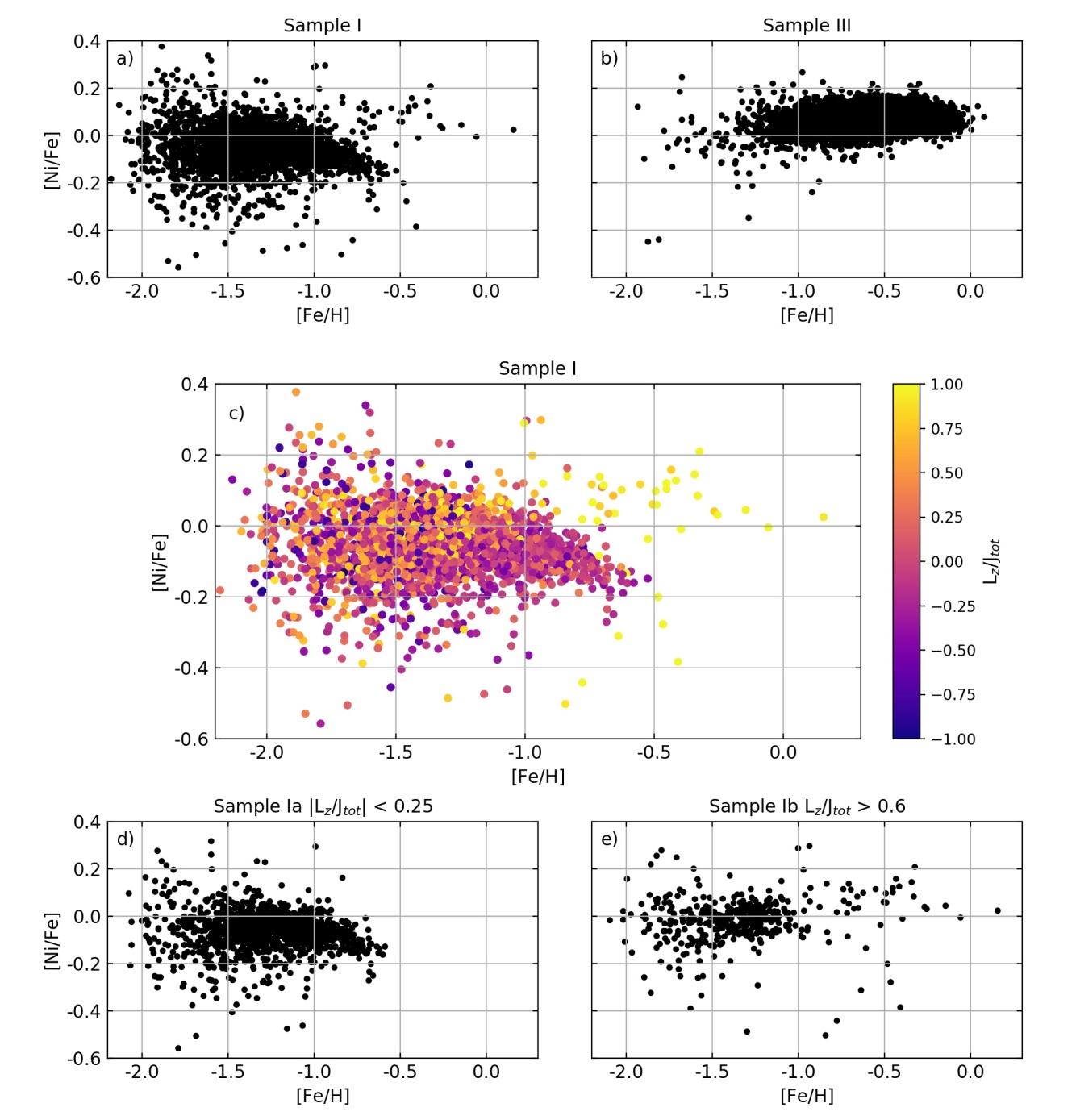
Apart from the -elements, nickel also shows the downward trend characteristic of Gaia-Sausage-Enceladus, as already demonstrated in Nissen & Schuster (1997, 2010). Fig. 19 shows the same elemental abundance plots as shown for [Mg/Fe] in Fig. 8 but for [Ni/Fe]. As can be seen, the resemblance is striking, further indicating that our analysis and conclusions are robust.
Appendix D The age of Sample III based on asteroseismic data
Table 8 provides the date for stars from Borre et al. (2022) that fall in our Sample III and fullfill the quaility criteria we apply (Table 1). The ages are from Borre et al. (2022) while the elemental abundances are taken from APOGEE DR17. We list the KIC/EPIC ID as given in Borre et al. (2022) and provde a cross-match to the Gaia DR3 IDs.
| KIC/EPIC | Gaia ID | [Fe/H] | [Mg/Fe] | Age | Age error |
|---|---|---|---|---|---|
| KIC 2571323 | 2051107025724208256 | –0.77 | 0.34 | 9.81 | 2.87 /–0.96 |
| KIC 2165615 | 2051825277390535552 | –0.73 | 0.36 | 2.45 | 0.67/–0.38 |
| KIC 2301577 | 2052544465376348416 | –0.45 | 0.31 | 3.67 | 0.74/–0.33 |
| KIC 5371173 | 2076546151381304448 | –0.51 | 0.33 | 9.43 | 0.45/–1.12 |
| KIC 7908109 | 2078761117553102208 | –0.75 | 0.35 | 9.80 | 1.50/–0.23 |
| KIC 11774651 | 2087261373224223616 | –0.43 | 0.32 | 13.18 | 0.71/–1.62 |
| KIC 5698156 | 2101432149662610816 | –1.27 | 0.31 | 12.80 | 1.52/–2.15 |
| KIC 5446927 | 2101503690937150464 | –0.74 | 0.13 | 4.90 | 7.37 -3.25 |
| KIC 6267115 | 2104059540072830336 | –0.35 | 0.31 | 8.12 | 1.80 -1.86 |
| KIC 7502070 | 2104862900816530432 | –0.59 | 0.33 | 9.25 | 2.68 -1.43 |
| KIC 7946809 | 2105698602672618752 | –0.54 | 0.33 | 7.04 | 2.88 -2.55 |
| KIC 8544630 | 2106715341689368320 | –0.58 | 0.32 | 8.32 | 1.43 -0.55 |
| KIC 10207078 | 2129106380594661248 | –0.31 | 0.33 | 9.40 | 0.66 -1.10 |
| KIC 12109442 | 2130163625443203328 | –0.54 | 0.38 | 12.05 | 1.76 -2.94 |
| KIC 10398120 | 2130915214660138624 | –0.99 | 0.34 | 8.59 | 1.35 -1.52 |
| KIC 12506245 | 2133443541646852864 | –0.71 | 0.31 | 12.75 | 0.78 -2.86 |
| EPIC 220387868 | 2551830805756981248 | –1.07 | 0.36 | 8.20 | 1.70 -1.88 |
| EPIC 220269276 | 2559320399792228096 | –0.31 | 0.29 | 4.33 | 2.87 -1.53 |
| EPIC 205997746 | 2596851370212990720 | –1.06 | 0.32 | 11.29 | 2.10 -1.90 |
| EPIC 205972576 | 2598768815412715776 | –0.35 | 0.26 | 11.62 | 2.30 -2.66 |
| EPIC 251512185 | 3684177626014911360 | –0.67 | 0.37 | 9.18 | 3.92 -4.38 |
| EPIC 204785972 | 4127168730546419072 | –0.46 | 0.30 | 7.34 | 4.39 -4.25 |
| EPIC 204298932 | 6050297413148822656 | –0.68 | 0.35 | 9.24 | 3.91 -3.11 |
| EPIC 205083494 | 6245695266654085888 | –1.01 | 0.36 | 8.17 | 1.80 -1.80 |
| EPIC 212297999 | 6293687295639821824 | –0.57 | 0.33 | 7.69 | 4.28 -3.30 |
| EPIC 213463719 | 6758726460165845248 | –0.07 | 0.22 | 13.19 | 1.40 -3.65 |
| EPIC 213523425 | 6759483817516180352 | –0.37 | 0.30 | 13.18 | 0.71 -2.35 |
| EPIC 213632986 | 6759511374026333568 | –0.57 | 0.38 | 6.98 | 5.01 -3.53 |
| EPIC 213853964 | 6759619023088186496 | –0.70 | 0.29 | 7.81 | 3.18 -1.98 |
| EPIC 213764390 | 6759773577490110464 | –0.36 | 0.25 | 5.32 | 1.66 -1.41 |
References
- Abdurro’uf et al. (2022) Abdurro’uf, Accetta, K., Aerts, C., et al. 2022, ApJS, 259, 35, doi: 10.3847/1538-4365/ac4414
- Ahumada et al. (2020) Ahumada, R., Prieto, C. A., Almeida, A., et al. 2020, ApJS, 249, 3, doi: 10.3847/1538-4365/ab929e
- Alexeeva et al. (2018) Alexeeva, S., Ryabchikova, T., Mashonkina, L., & Hu, S. 2018, ApJ, 866, 153, doi: 10.3847/1538-4357/aae1a8
- Amarante et al. (2020) Amarante, J. A. S., Beraldo e Silva, L., Debattista, V. P., & Smith, M. C. 2020, ApJ, 891, L30, doi: 10.3847/2041-8213/ab78a4
- Amarsi et al. (2022) Amarsi, A. M., Liljegren, S., & Nissen, P. E. 2022, A&A, 668, A68, doi: 10.1051/0004-6361/202244542
- Amarsi et al. (2016) Amarsi, A. M., Lind, K., Asplund, M., Barklem, P. S., & Collet, R. 2016, MNRAS, 463, 1518, doi: 10.1093/mnras/stw2077
- Andrews et al. (2017) Andrews, B. H., Weinberg, D. H., Schönrich, R., & Johnson, J. A. 2017, ApJ, 835, 224, doi: 10.3847/1538-4357/835/2/224
- Arnett (1996) Arnett, D. 1996, Supernovae and Nucleosynthesis: An Investigation of the History of Matter from the Big Bang to the Present
- Astropy Collaboration et al. (2013) Astropy Collaboration, Robitaille, T. P., Tollerud, E. J., et al. 2013, A&A, 558, A33, doi: 10.1051/0004-6361/201322068
- Astropy Collaboration et al. (2018) Astropy Collaboration, Price-Whelan, A. M., Sipőcz, B. M., et al. 2018, AJ, 156, 123, doi: 10.3847/1538-3881/aabc4f
- Bailer-Jones et al. (2021) Bailer-Jones, C. A. L., Rybizki, J., Fouesneau, M., Demleitner, M., & Andrae, R. 2021, AJ, 161, 147, doi: 10.3847/1538-3881/abd806
- Battistini & Bensby (2016) Battistini, C., & Bensby, T. 2016, A&A, 586, A49, doi: 10.1051/0004-6361/201527385
- Belokurov (2013) Belokurov, V. 2013, New A Rev., 57, 100, doi: 10.1016/j.newar.2013.07.001
- Belokurov et al. (2018) Belokurov, V., Erkal, D., Evans, N. W., Koposov, S. E., & Deason, A. J. 2018, MNRAS, 478, 611, doi: 10.1093/mnras/sty982
- Belokurov et al. (2020) Belokurov, V., Sanders, J. L., Fattahi, A., et al. 2020, MNRAS, 494, 3880, doi: 10.1093/mnras/staa876
- Belokurov et al. (2006) Belokurov, V., Zucker, D. B., Evans, N. W., et al. 2006, ApJ, 642, L137, doi: 10.1086/504797
- Bensby et al. (2014) Bensby, T., Feltzing, S., & Oey, M. S. 2014, A&A, 562, A71, doi: 10.1051/0004-6361/201322631
- Bergemann et al. (2017) Bergemann, M., Collet, R., Amarsi, A. M., et al. 2017, ApJ, 847, 15, doi: 10.3847/1538-4357/aa88cb
- Bergemann et al. (2012) Bergemann, M., Lind, K., Collet, R., Magic, Z., & Asplund, M. 2012, MNRAS, 427, 27, doi: 10.1111/j.1365-2966.2012.21687.x
- Bergemann et al. (2019) Bergemann, M., Gallagher, A. J., Eitner, P., et al. 2019, A&A, 631, A80, doi: 10.1051/0004-6361/201935811
- Binney (2012) Binney, J. 2012, MNRAS, 426, 1324, doi: 10.1111/j.1365-2966.2012.21757.x
- Bland-Hawthorn & Gerhard (2016) Bland-Hawthorn, J., & Gerhard, O. 2016, ARA&A, 54, 529, doi: 10.1146/annurev-astro-081915-023441
- Bonifacio et al. (2009) Bonifacio, P., Spite, M., Cayrel, R., et al. 2009, A&A, 501, 519, doi: 10.1051/0004-6361/200810610
- Borre et al. (2022) Borre, C. C., Aguirre Børsen-Koch, V., Helmi, A., et al. 2022, MNRAS, 514, 2527, doi: 10.1093/mnras/stac1498
- Bovy (2015) Bovy, J. 2015, ApJS, 216, 29, doi: 10.1088/0067-0049/216/2/29
- Bovy & Rix (2013) Bovy, J., & Rix, H.-W. 2013, ApJ, 779, 115, doi: 10.1088/0004-637X/779/2/115
- Buder et al. (2018) Buder, S., Asplund, M., Duong, L., et al. 2018, MNRAS, 478, 4513, doi: 10.1093/mnras/sty1281
- Buder et al. (2021) Buder, S., Sharma, S., Kos, J., et al. 2021, MNRAS, 506, 150, doi: 10.1093/mnras/stab1242
- Chiappini et al. (2015) Chiappini, C., Anders, F., Rodrigues, T. S., et al. 2015, A&A, 576, L12, doi: 10.1051/0004-6361/201525865
- Das et al. (2020) Das, P., Hawkins, K., & Jofré, P. 2020, MNRAS, 493, 5195, doi: 10.1093/mnras/stz3537
- Di Matteo et al. (2019) Di Matteo, P., Haywood, M., Lehnert, M. D., et al. 2019, A&A, 632, A4, doi: 10.1051/0004-6361/201834929
- Fernandes et al. (2023) Fernandes, L., Mason, A. C., Horta, D., et al. 2023, MNRAS, 519, 3611, doi: 10.1093/mnras/stac3543
- Feuillet et al. (2020) Feuillet, D. K., Feltzing, S., Sahlholdt, C. L., & Casagrande, L. 2020, MNRAS, 497, 109, doi: 10.1093/mnras/staa188810.48550/arXiv.2003.11039
- Feuillet et al. (2021) Feuillet, D. K., Sahlholdt, C. L., Feltzing, S., & Casagrande, L. 2021, MNRAS, 508, 1489, doi: 10.1093/mnras/stab2614
- Forbes (2020) Forbes, D. A. 2020, MNRAS, 493, 847, doi: 10.1093/mnras/staa245
- Freeman & Bland-Hawthorn (2002) Freeman, K., & Bland-Hawthorn, J. 2002, ARA&A, 40, 487, doi: 10.1146/annurev.astro.40.060401.093840
- Gaia Collaboration et al. (2016a) Gaia Collaboration, Brown, A. G. A., Vallenari, A., et al. 2016a, A&A, 595, A2, doi: 10.1051/0004-6361/201629512
- Gaia Collaboration et al. (2016b) Gaia Collaboration, Prusti, T., de Bruijne, J. H. J., et al. 2016b, A&A, 595, A1, doi: 10.1051/0004-6361/201629272
- Gaia Collaboration et al. (2018a) Gaia Collaboration, Brown, A. G. A., Vallenari, A., et al. 2018a, A&A, 616, A1, doi: 10.1051/0004-6361/201833051
- Gaia Collaboration et al. (2018b) Gaia Collaboration, Babusiaux, C., van Leeuwen, F., et al. 2018b, A&A, 616, A10, doi: 10.1051/0004-6361/201832843
- Gaia Collaboration et al. (2021) Gaia Collaboration, Brown, A. G. A., Vallenari, A., et al. 2021, A&A, 649, A1, doi: 10.1051/0004-6361/202039657
- Gallart et al. (2019) Gallart, C., Bernard, E. J., Brook, C. B., et al. 2019, Nature Astronomy, 3, 932, doi: 10.1038/s41550-019-0829-5
- Hammer et al. (2023) Hammer, F., Li, H., Mamon, G. A., et al. 2023, MNRAS, 519, 5059, doi: 10.1093/mnras/stac3758
- Hasselquist et al. (2021) Hasselquist, S., Hayes, C. R., Lian, J., et al. 2021, ApJ, 923, 172, doi: 10.3847/1538-4357/ac25f9
- Hawkins et al. (2015) Hawkins, K., Jofré, P., Masseron, T., & Gilmore, G. 2015, MNRAS, 453, 758, doi: 10.1093/mnras/stv1586
- Hayes et al. (2018) Hayes, C. R., Majewski, S. R., Shetrone, M., et al. 2018, ApJ, 852, 49, doi: 10.3847/1538-4357/aa9cec
- Hayes et al. (2020) Hayes, C. R., Majewski, S. R., Hasselquist, S., et al. 2020, ApJ, 889, 63, doi: 10.3847/1538-4357/ab62ad
- Haywood et al. (2018) Haywood, M., Di Matteo, P., Lehnert, M. D., et al. 2018, ApJ, 863, 113, doi: 10.3847/1538-4357/aad235
- Heiter & Eriksson (2006) Heiter, U., & Eriksson, K. 2006, A&A, 452, 1039, doi: 10.1051/0004-6361:20064925
- Helmi (2020) Helmi, A. 2020, ARA&A, 58, 205, doi: 10.1146/annurev-astro-032620-021917
- Helmi et al. (2018) Helmi, A., Babusiaux, C., Koppelman, H. H., et al. 2018, Nature, 563, 85, doi: 10.1038/s41586-018-0625-x
- Helmi et al. (1999) Helmi, A., White, S. D. M., de Zeeuw, P. T., & Zhao, H. 1999, Nature, 402, 53, doi: 10.1038/46980
- Horta et al. (2021) Horta, D., Schiavon, R. P., Mackereth, J. T., et al. 2021, MNRAS, 500, 1385, doi: 10.1093/mnras/staa2987
- Horta et al. (2022) —. 2022, MNRAS, doi: 10.1093/mnras/stac3179
- Jofré et al. (2016) Jofré, P., Jorissen, A., Van Eck, S., et al. 2016, A&A, 595, A60, doi: 10.1051/0004-6361/201629356
- Jönsson et al. (2020) Jönsson, H., Holtzman, J. A., Allende Prieto, C., et al. 2020, AJ, 160, 120, doi: 10.3847/1538-3881/aba592
- Khoperskov et al. (2022a) Khoperskov, S., Minchev, I., Libeskind, N., et al. 2022a, arXiv e-prints, arXiv:2206.04521, doi: 10.48550/arXiv.2206.04521
- Khoperskov et al. (2022b) —. 2022b, arXiv e-prints, arXiv:2206.04522, doi: 10.48550/arXiv.2206.04522
- Khoperskov et al. (2022c) —. 2022c, arXiv e-prints, arXiv:2206.05491. https://arxiv.org/abs/2206.05491
- Kobayashi et al. (2020) Kobayashi, C., Karakas, A. I., & Lugaro, M. 2020, ApJ, 900, 179, doi: 10.3847/1538-4357/abae65
- Koch et al. (2013) Koch, A., Feltzing, S., Adén, D., & Matteucci, F. 2013, A&A, 554, A5, doi: 10.1051/0004-6361/201220742
- Koppelman et al. (2019) Koppelman, H. H., Helmi, A., Massari, D., Price-Whelan, A. M., & Starkenburg, T. K. 2019, A&A, 631, L9, doi: 10.1051/0004-6361/201936738
- Kruijssen et al. (2019) Kruijssen, J. M. D., Pfeffer, J. L., Reina-Campos, M., Crain, R. A., & Bastian, N. 2019, MNRAS, 486, 3180, doi: 10.1093/mnras/sty1609
- Lambert (1989) Lambert, D. L. 1989, in American Institute of Physics Conference Series, Vol. 183, Cosmic Abundances of Matter, ed. C. J. Waddington, 168–199, doi: 10.1063/1.38011
- Lane et al. (2022) Lane, J. M. M., Bovy, J., & Mackereth, J. T. 2022, MNRAS, 510, 5119, doi: 10.1093/mnras/stab3755
- Libeskind et al. (2020) Libeskind, N. I., Carlesi, E., Grand, R. J. J., et al. 2020, MNRAS, 498, 2968, doi: 10.1093/mnras/staa2541
- Lind et al. (2012) Lind, K., Bergemann, M., & Asplund, M. 2012, MNRAS, 427, 50, doi: 10.1111/j.1365-2966.2012.21686.x
- Majewski et al. (2017) Majewski, S. R., Schiavon, R. P., Frinchaboy, P. M., et al. 2017, AJ, 154, 94, doi: 10.3847/1538-3881/aa784d
- Malhan et al. (2022) Malhan, K., Ibata, R. A., Sharma, S., et al. 2022, ApJ, 926, 107, doi: 10.3847/1538-4357/ac4d2a
- Massari et al. (2019) Massari, D., Koppelman, H. H., & Helmi, A. 2019, A&A, 630, L4, doi: 10.1051/0004-6361/201936135
- Masseron et al. (2021) Masseron, T., Osorio, Y., García-Hernández, D. A., et al. 2021, A&A, 647, A24, doi: 10.1051/0004-6361/202039484
- Matteucci (2012) Matteucci, F. 2012, Chemical Evolution of Galaxies, doi: 10.1007/978-3-642-22491-1
- McMillan (2017) McMillan, P. J. 2017, MNRAS, 465, 76, doi: 10.1093/mnras/stw2759
- McWilliam (1997) McWilliam, A. 1997, ARA&A, 35, 503, doi: 10.1146/annurev.astro.35.1.503
- Miglio et al. (2017) Miglio, A., Chiappini, C., Mosser, B., et al. 2017, Astronomische Nachrichten, 338, 644, doi: 10.1002/asna.201713385
- Miglio et al. (2021) Miglio, A., Chiappini, C., Mackereth, J. T., et al. 2021, A&A, 645, A85, doi: 10.1051/0004-6361/202038307
- Mints & Hekker (2019) Mints, A., & Hekker, S. 2019, A&A, 621, A17, doi: 10.1051/0004-6361/201834256
- Montalbán et al. (2021) Montalbán, J., Mackereth, J. T., Miglio, A., et al. 2021, Nature Astronomy, 5, 640, doi: 10.1038/s41550-021-01347-7
- Myeong et al. (2019) Myeong, G. C., Vasiliev, E., Iorio, G., Evans, N. W., & Belokurov, V. 2019, MNRAS, 488, 1235, doi: 10.1093/mnras/stz1770
- Naidu et al. (2020) Naidu, R. P., Conroy, C., Bonaca, A., et al. 2020, ApJ, 901, 48, doi: 10.3847/1538-4357/abaef4
- Naidu et al. (2022) Naidu, R. P., Ji, A. P., Conroy, C., et al. 2022, ApJ, 926, L36, doi: 10.3847/2041-8213/ac5589
- Nissen & Schuster (1997) Nissen, P. E., & Schuster, W. J. 1997, A&A, 326, 751
- Nissen & Schuster (2010) —. 2010, A&A, 511, L10, doi: 10.1051/0004-6361/200913877
- Nomoto et al. (1997) Nomoto, K., Iwamoto, K., Nakasato, N., et al. 1997, Nucl. Phys. A, 621, 467, doi: 10.1016/S0375-9474(97)00291-1
- Nordlander & Lind (2017) Nordlander, T., & Lind, K. 2017, A&A, 607, A75, doi: 10.1051/0004-6361/201730427
- Osorio et al. (2020) Osorio, Y., Allende Prieto, C., Hubeny, I., Mészáros, S., & Shetrone, M. 2020, A&A, 637, A80, doi: 10.1051/0004-6361/201937054
- Pagnini et al. (2023) Pagnini, G., Di Matteo, P., Khoperskov, S., et al. 2023, A&A, 673, A86, doi: 10.1051/0004-6361/202245128
- Roederer et al. (2016) Roederer, I. U., Mateo, M., Bailey, John I., I., et al. 2016, AJ, 151, 82, doi: 10.3847/0004-6256/151/3/82
- Sahlholdt et al. (2019a) Sahlholdt, C. L., Casagrande, L., & Feltzing, S. 2019a, ApJ, 881, L10, doi: 10.3847/2041-8213/ab321e
- Sahlholdt et al. (2019b) Sahlholdt, C. L., Feltzing, S., Lindegren, L., & Church, R. P. 2019b, MNRAS, 482, 895, doi: 10.1093/mnras/sty2732
- Shetrone et al. (2015) Shetrone, M., Bizyaev, D., Lawler, J. E., et al. 2015, ApJS, 221, 24, doi: 10.1088/0067-0049/221/2/24
- Smith et al. (2021) Smith, V. V., Bizyaev, D., Cunha, K., et al. 2021, AJ, 161, 254, doi: 10.3847/1538-3881/abefdc
- Soderblom (2010) Soderblom, D. R. 2010, ARA&A, 48, 581, doi: 10.1146/annurev-astro-081309-130806
- Stonkutė et al. (2016) Stonkutė, E., Koposov, S. E., Howes, L. M., et al. 2016, MNRAS, 460, 1131, doi: 10.1093/mnras/stw1011
- Tolstoy et al. (2009) Tolstoy, E., Hill, V., & Tosi, M. 2009, ARA&A, 47, 371, doi: 10.1146/annurev-astro-082708-101650
- Vasiliev (2019) Vasiliev, E. 2019, MNRAS, 484, 2832, doi: 10.1093/mnras/stz171
- Weinberg et al. (2019) Weinberg, D. H., Holtzman, J. A., Hasselquist, S., et al. 2019, ApJ, 874, 102, doi: 10.3847/1538-4357/ab07c7
- Zhang et al. (2017) Zhang, J., Shi, J., Pan, K., Allende Prieto, C., & Liu, C. 2017, ApJ, 835, 90, doi: 10.3847/1538-4357/835/1/90