Planetary line-to-accretion luminosity scaling relations: Extrapolating to higher-order hydrogen lines

Abstract

Aoyama et al. (2021) provided scaling relations between hydrogen-line luminosities and the accretion luminosity for planetary-mass objects. These fits should be an improvement over blind extrapolations of stellar relations. The fits go up only to the $n=8$ electron energy level, but higher-$n$ Balmer lines have been observed in the near-UV at Delorme 1 (AB)b with UVES (Ringqvist et al., 2023). We extend the scaling relations to higher-$n$ levels for the Balmer and other series by fitting the fit coefficients $(a,b)$ themselves and extrapolating them. Within the assumption of an accretion shock as the source of line emission, these fits should be robust for accreting planetary-mass objects.

9 December 2022 at RNAAS

1 Motivation

Planetary-mass companions have been detected or observed at emission lines (e.g., Haffert et al., 2019; Wu et al., 2022; Betti et al., 2022a, b; Ringqvist et al., 2023). As for Classical T Tauri Stars (CTTSs), the lines trace the accretion process, and should originate from an accretion shock, magnetospheric accretion columns, or both (Aoyama et al., 2021; hereafter Ao21). Empirically, each line luminosity $L_{\mathrm{line}}$ correlates with total accretion luminosity ${L_{\textnormal{acc}}}$, which is set mostly by the accretion rate $\dot{M}$. Thus, emission-line observations yield constraints on the formation mechanism and formation timescale of the accretors.

Different models attempt to convert emission-line luminosities into an accretion rate (Aoyama et al., 2018, 2020; Aoyama & Ikoma, 2019; Ao21; Thanathibodee et al., 2019; Szulágyi & Ercolano, 2020; Dong et al., 2021). A popular approach extrapolates the empirical ${L_{\textnormal{acc}}}$–$L_{\mathrm{line}}$ correlation for CTTSs (e.g., Rigliaco et al., 2012; Alcalá et al., 2017; Komarova & Fischer, 2020) down to planetary masses. In Ao21, we pointed out that at $\mathrm{H}\,\alpha$ luminosities $L_{\textnormal{H}\,\alpha}\lesssim 10^{-6}~{}{L_{\odot}}$ (near the $L_{\textnormal{H}\,\alpha}$ of PDS 70 b; Zhou et al., 2021), extrapolating Rigliaco et al. (2012) predicts more $\mathrm{H}\,\alpha$ emission than incoming energy. Thus, blind extrapolations might be invalid.

In Ao21 we gave $L_{\mathrm{line}}$–${L_{\textnormal{acc}}}$ scaling relations meant to apply at planetary masses. They are based on a simplified model of the accretion geometry but combined with detailed, NLTE hydrogen-line emission calculations (Aoyama et al., 2018). We computed and fit ${L_{\textnormal{acc}}}$ only up to the $n=8$ energy level since the microphysical model follows electron populations only up to a certain level.

UVES observations of Delorme 1 (AB)b (Ringqvist et al., 2023) motivate us to extend the relationships to higher $n$, thinking also of CUBES (Alcalá et al., 2022) or NIR instruments. We fit the fit coefficients of our existing relations and extrapolate them to higher-order lines.

2 Fit of the fit coefficients, and their extrapolation

Figure 1: Fit coefficients of the planetary ${L_{\textnormal{acc}}}$–$L_{\mathrm{line}}$ relation (Eq. (1)) for Lyman ($n_{\mathrm{f}}=1$) to Brackett ($n_{\mathrm{f}}=4$) lines. Circles: direct fits of ${L_{\textnormal{acc}}}$–$L_{\mathrm{line}}$ (Ao21 and see text). Black lines: our fit of the fit coefficients $a$ and $b$ (Eq. (2)). Golden squares: Alcalá et al. (2017) for Balmer lines.

The correlation between ${L_{\textnormal{acc}}}$ and each $L_{\mathrm{line}}$ is usually written as (e.g., Alcalá et al., 2017)

$$\log_{10}\left({L_{\textnormal{acc}}}/{L_{\odot}}\right)=a\times\log_{10}\left(L_{\mathrm{line}}/{L_{\odot}}\right)+b,$$ (1)

with $a$ and $b$ the fit coefficients. In Ao21, we considered a range of planet masses and accretion rates and fit the resulting $L_{\mathrm{line}}({L_{\textnormal{acc}}})$. A hydrogen line is defined by the starting and final electron energy levels, $n_{\mathrm{i}}$ and $n_{\mathrm{f}}$. Since the Aoyama et al. (2018) models go only up to $n=10$, we did not study lines beyond $n_{\mathrm{i}}=8$ to avoid possible “edge effects”. However, higher-level lines are in fact reliable enough (see §3). Therefore we generate $L_{\mathrm{line}}$ as in Ao21 for an ($\dot{M}$, mass) grid for H9, H10, Pa9, Pa10, and Br9, and fit Eq. (1) to obtain their $a$ and $b$.

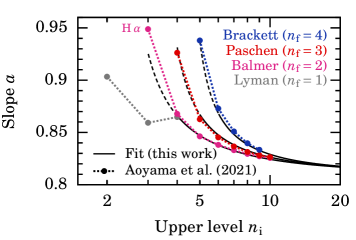
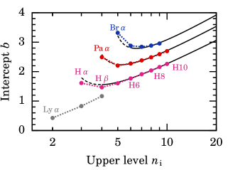
Next, we plot the $a$ and $b$ of all lines as a function of $n_{\mathrm{i}}$ and $n_{\mathrm{f}}$ (Fig. 1). We tried different functional forms, fitting the free parameters through gnuplot. We used only the $n_{\mathrm{f}}=2$–4 series, excluded the first ($\alpha$) transition of each, and weighted by $1/(n_{\mathrm{i}}-n_{\mathrm{f}})$. The goal was to have a reliable extrapolation beyond $n\approx 10$ (from Ao21 or the lines added above). An excellent fit is:

$$a(n_{\mathrm{i}},n_{\mathrm{f}})= 0.811-\frac{1}{9.90n_{\mathrm{f}}-9.5n_{\mathrm{i}}}$$ (2a)

$$b(n_{\mathrm{i}},n_{\mathrm{f}})= \left[1+1.05\ln(n_{\mathrm{i}})+\frac{1}{n_{\mathrm{i}}-n_{\mathrm{f}}}-\frac{1}{n_{\mathrm{f}}}\right]$$

$$\times(1.07+0.0694n_{\mathrm{f}})-1.41.$$ (2b)

Even though we excluded the $\alpha$ lines, their $(a,b)$ predicted by Eq. (2) agree closely with the ones from the direct fits.

Thus, examples of planetary-regime scaling relations extending those of Ao21 are:

$$\log_{10}({L_{\textnormal{acc}}}/{L_{\odot}}) =0.83\log_{10}(L_{\mathrm{H9}}/{L_{\odot}})+2.16$$ (3)

$$\log_{10}({L_{\textnormal{acc}}}/{L_{\odot}}) =0.82\log_{10}(L_{\mathrm{H10}}/{L_{\odot}})+2.27$$ (4)

$$\log_{10}({L_{\textnormal{acc}}}/{L_{\odot}}) =0.82\log_{10}(L_{\mathrm{H11}}/{L_{\odot}})+2.37$$ (5)

$$\log_{10}({L_{\textnormal{acc}}}/{L_{\odot}}) =0.82\log_{10}(L_{\mathrm{H12}}/{L_{\odot}})+2.47$$ (6)

$$\log_{10}({L_{\textnormal{acc}}}/{L_{\odot}}) =0.82\log_{10}(L_{\mathrm{H13}}/{L_{\odot}})+2.56$$ (7)

$$\log_{10}({L_{\textnormal{acc}}}/{L_{\odot}}) =0.82\log_{10}(L_{\mathrm{H14}}/{L_{\odot}})+2.64$$ (8)

$$\log_{10}({L_{\textnormal{acc}}}/{L_{\odot}}) =0.82\log_{10}(L_{\mathrm{H15}}/{L_{\odot}})+2.72$$ (9)

$$\log_{10}({L_{\textnormal{acc}}}/{L_{\odot}}) =0.82\log_{10}(L_{\mathrm{H16}}/{L_{\odot}})+2.80,$$ (10)

$$\log_{10}({L_{\textnormal{acc}}}/{L_{\odot}}) =0.83\log_{10}(L_{\mathrm{Pa9}}/{L_{\odot}})+2.60$$ (11)

$$\log_{10}({L_{\textnormal{acc}}}/{L_{\odot}}) =0.83\log_{10}(L_{\mathrm{Pa10}}/{L_{\odot}})+2.72$$ (12)

$$\log_{10}({L_{\textnormal{acc}}}/{L_{\odot}}) =0.82\log_{10}(L_{\mathrm{Pa11}}/{L_{\odot}})+2.82$$ (13)

$$\log_{10}({L_{\textnormal{acc}}}/{L_{\odot}}) =0.82\log_{10}(L_{\mathrm{Pa12}}/{L_{\odot}})+2.92$$ (14)

$$\log_{10}({L_{\textnormal{acc}}}/{L_{\odot}}) =0.82\log_{10}(L_{\mathrm{Pa13}}/{L_{\odot}})+3.01,$$ (15)

$$\log_{10}({L_{\textnormal{acc}}}/{L_{\odot}}) =0.83\log_{10}(L_{\mathrm{Br9}}/{L_{\odot}})+2.98$$ (16)

$$\log_{10}({L_{\textnormal{acc}}}/{L_{\odot}}) =0.83\log_{10}(L_{\mathrm{Br10}}/{L_{\odot}})+3.08$$ (17)

$$\log_{10}({L_{\textnormal{acc}}}/{L_{\odot}}) =0.83\log_{10}(L_{\mathrm{Br11}}/{L_{\odot}})+3.19$$ (18)

$$\log_{10}({L_{\textnormal{acc}}}/{L_{\odot}}) =0.82\log_{10}(L_{\mathrm{Br12}}/{L_{\odot}})+3.29,$$ (19)

simply evaluating Eq. (2) for $n_{\mathrm{f}}=2$–4 and several $n_{\mathrm{i}}$ as examples. Where $(a,b)$ from direct fits are available, the coefficients match excellently. Especially since the $(a,b)$ capture only an average relation, Eq. (2) can also be used for the Pfund or other series ($n_{\mathrm{f}}\geqslant 5$).

For error propagation, the errorbar on ${L_{\textnormal{acc}}}$ is $\sigma\approx 0.3$ dex as for the other lines (Appendix A of Ao21). The species toolkit includes Eqs. (3)–(19) (Stolker et al., 2020; “Emission line” tutorial at https://species.readthedocs.io).

3 Discussion

A few points deserve discussion:

1. Why does it work?—The lines originate from the shock-heated gas below the shock. There, the cooling is slower than or comparable to the electron transitions from low-$n$ levels. This makes non-equilibrium calculations necessary (Aoyama et al., 2018). However, contrary to the transitions from low-$n$ levels that have a large energy difference, the transitions between high-$n$ levels are faster than the cooling by more than orders of magnitudes. Thus, highly-excited-hydrogen abundances follow the thermal (Boltzmann) distribution, which is monotonic, essentially exponential. At velocities and densities relevant here (Aoyama et al., 2020), electrons with $n\gtrsim 7$ are thermally equilibrated. Correspondingly, the line strength of transitions from those $n$ is a simple function. The limiting behaviour seen in Fig. 1 reflects this.

2. Domain of validity—All slopes in all series converge to $a\approx 0.82$, whereas the intercepts are $b\approx 2$–3, growing roughly logarithmically (Eq. (2)). This increase of $b$ reflects the intuitive result that a diminishing fraction of ${L_{\textnormal{acc}}}$ goes into lines of higher energy within a series ($L_{\mathrm{line}}/{L_{\textnormal{acc}}}\sim 10^{-b}$ since $a\sim 1$). Formally, integrating $L_{\mathrm{line}}$ from $n_{\mathrm{f}}$ to infinity diverges, but actually Eq. (2) will hold only below a maximum $n_{\mathrm{i}}$. The highest observable $n_{\mathrm{i}}$ is likely small than this anyway.

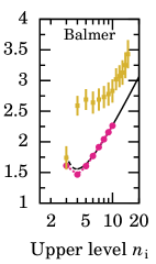
3. Compared to stars?—In the CTTS relations of Alcalá et al. (2017), $a_{\star}\approx 1.0$–1.1 while $b_{\star}\approx 2.8$–3.6, also increasing with $n_{\mathrm{i}}$ (Fig. 1). At $L_{\mathrm{line}}$ values where the stellar and the planetary regimes somewhat overlap, this leads to a major, 1–4 dex discrepancy in ${L_{\textnormal{acc}}}$ between the two approaches (Ao21). In the planetary-shock case, a much smaller fraction of the kinetic energy is converted into line luminosity.

4. Physical context—The fits apply to shock emission, whether from magnetospheric or purely hydrodynamic accretion onto the surface of a planet or its CPD. However, no emission from accretion columns themselves is considered (Ao21). Constraining their temperature structure observationally (Petrov et al., 2014) or theoretically would enable estimating their contribution.

5. Which way forward?—The model of Aoyama et al. (2018) could be extended to calculate directly hydrogen lines involving $n>10$ electrons, but for the purposes of ${L_{\textnormal{acc}}}$–$L_{\mathrm{line}}$ relations our extrapolations should more than suffice. Adding He and metal lines would matter more. At preshock velocities $v_{0}\gtrsim 200$ km s^-1, they and the hydrogen continuum carry a sizeable fraction of the energy (Aoyama et al., 2020), and have been detected (Eriksson et al., 2020; Zhou et al., 2021; Betti et al., 2022a, b; Ringqvist et al., 2023).

4 Summary

In Ao21, we derived ${L_{\textnormal{acc}}}$–$L_{\mathrm{line}}$ scalings for accreting planets. These scalings should replace uncalibrated extrapolations of the stellar relations down to low line luminosities, which can yield unphysical results. Here, we fit the fit coefficients for the Balmer, Paschen, and Brackett series and extrapolated them to higher-level lines. Thanks to the simplicity of the hydrogen atom, we argued that this estimates well the results of detailed calculations, also for higher series. The underlying scenario is a shock in which hydrogen lines carry most of the energy. Thus this extension is valid in the same domain of preshock conditions as the main model: for preshock number densities $n_{0}\sim 10^{9}$–$10^{14}$ cm^-3 and preshock velocities up to $v_{0}\approx 200$ km s^-1 (Aoyama et al., 2020). Eq. (2) can be used to generate scalings easily, with examples in Eqs. (3)–(19). These extended relations allow estimates of the accretion rate of planetary-mass objects from even more hydrogen lines than up to now.

References

- Alcalá et al. (2022) Alcalá, J. M., Cupani, G., Evans, C. J., Franchini, M., & Nisini, B. 2022, Experimental Astronomy, arXiv:2203.15581
- Alcalá et al. (2017) Alcalá, J. M., Manara, C. F., Natta, A., et al. 2017, A&A, 600, A20
- Aoyama & Ikoma (2019) Aoyama, Y., & Ikoma, M. 2019, ApJ, 885, L29
- Aoyama et al. (2018) Aoyama, Y., Ikoma, M., & Tanigawa, T. 2018, ApJ, 866, 84
- Aoyama et al. (2021) Aoyama, Y., Marleau, G.-D., Ikoma, M., & Mordasini, C. 2021, ApJ, 917, L30
- Aoyama et al. (2020) Aoyama, Y., Marleau, G.-D., Mordasini, C., & Ikoma, M. 2020, arXiv e-prints, arXiv:2011.06608
- Betti et al. (2022b) Betti, S. K., Follette, K. B., Ward-Duong, K., et al. 2022a, ApJ, 935, L18
- Betti et al. (2022a) Betti, S. K., Follette, K. B., Ward-Duong, K., et al. 2022b, ApJ, 941, L20
- Dong et al. (2021) Dong, J., Jiang, Y.-F., & Armitage, P. J. 2021, ApJ, 921, 54
- Eriksson et al. (2020) Eriksson, S. C., Asensio Torres, R., Janson, M., et al. 2020, A&A, 638, L6
- Haffert et al. (2019) Haffert, S., Bohn, A., de Boer, J., et al. 2019, Nat. Astron., 3, 749
- Komarova & Fischer (2020) Komarova, O., & Fischer, W. J. 2020, RNAAS, 4, 6
- Petrov et al. (2014) Petrov, P. P., Gahm, G. F., Herczeg, G. J., Stempels, H. C., & Walter, F. M. 2014, A&A, 568, L10
- Rigliaco et al. (2012) Rigliaco, E., Natta, A., Testi, L., et al. 2012, A&A, 548, A56
- Ringqvist et al. (2023) Ringqvist, S. C., Viswanath, G., Aoyama, Y., et al. 2023, A&A, 669, L12
- Stolker et al. (2020) Stolker, T., Quanz, S., Todorov, K., et al. 2020, A&A, 635, A182
- Szulágyi & Ercolano (2020) Szulágyi, J., & Ercolano, B. 2020, ApJ, 902, 126
- Thanathibodee et al. (2019) Thanathibodee, T., Calvet, N., Bae, J., Muzerolle, J., & Hernández, R. F. 2019, ApJ, 885, 94
- Wu et al. (2022) Wu, Y.-L., Bowler, B. P., Sheehan, P. D., et al. 2022, ApJ, 930, L3
- Zhou et al. (2021) Zhou, Y., Bowler, B. P., Wagner, K. R., et al. 2021, AJ, 161, 244