Stability of the Lanczos algorithm on matrices with regular spectral distributions

Abstract

We study the stability of the Lanczos algorithm run on problems whose eigenvector empirical spectral distribution is near to a reference measure with well-behaved orthogonal polynomials. We give a backwards stability result which can be upgraded to a forward stability result when the reference measure has a density supported on a single interval with square root behavior at the endpoints. Our analysis implies the Lanczos algorithm run on many large random matrix models is in fact forward stable, and hence nearly deterministic, even when computations are carried out in finite precision arithmetic. Since the Lanczos algorithm is not forward stable in general, this provides yet another example of the fact that random matrices are far from “any old matrix”, and care must be taken when using them to test numerical algorithms.

1 Introduction

The Lanczos algorithm is unstable in the sense that, even on the simplest problems, the output of the algorithm in finite precision arithmetic may be very different than what would have been obtained in exact arithmetic. Despite this, the Lanczos algorithm is among the most important algorithms in numerical linear algebra and is commonly used for a wide variety of fundamental linear-algebraic tasks including approximating eigenvalues and eigenvectors, the product of a matrix function on a vector, and quadratic forms involving matrix functions. Understanding the behavior of the Lanczos algorithm in finite precision arithmetic has been of interest since the introduction of the algorithm some 70 years ago [lanczos_50, golub_oleary_89, parlett_98, meurant_06, carson_liesen_strakos_22].

Algorithm 1 Lanczos algorithm

1:procedure Lanczos($\mathbf{A},\mathbf{b},k$)

2:     $\mathbf{q}_{0}=\mathbf{b}/\|\mathbf{b}\|$, $\beta_{-1}=0$, $\mathbf{q}_{-1}=\mathbf{0}$

3:     for $n=0,1,\ldots,k-1$ do

4:         $\tilde{\mathbf{q}}_{n+1}=\mathbf{A}\mathbf{q}_{n}-\beta_{n-1}\mathbf{q}_{n-1}$

5:         $\alpha_{n}=\tilde{\mathbf{q}}_{n+1}^{\mathsf{T}}\mathbf{q}_{n}$

6:         $\hat{\mathbf{q}}_{n+1}=\tilde{\mathbf{q}}_{n+1}-\alpha_{n}\mathbf{q}_{i}$

7:         $\beta_{n}=\|\hat{\mathbf{q}}_{n+1}\|$

8:         $\mathbf{q}_{n+1}=\hat{\mathbf{q}}_{n+1}/\beta_{n}$

9:     end for

10:end procedure

Throughout, $\mathbf{A}$ will be an $N\times N$ real symmetric matrix and $\mathbf{b}$ a unit-norm vector of length $N$. From $(\mathbf{A},\mathbf{b})$ we obtain the eigenvector empirical spectral distribution (VESD) defined by

$$\hyperref@@ii[eqn:VESD]{\color[rgb]{0,0,0}\mu_{N}}(\mathrm{d}{x})=\hyperref@@ii[eqn:VESD]{\color[rgb]{0,0,0}\mu_{\textup{VESD}}}(\mathrm{d}{x};\mathbf{A},\mathbf{b}):=\sum_{n=1}^{N}(\mathbf{b}^{\mathsf{T}}\mathbf{u}_{n})^{2}\>\delta_{\lambda_{n}}(\mathrm{d}x),$$ (1.1)

where $(\lambda_{n},\mathbf{u}_{n})$ are the eigenvalue-vector pairs of $\mathbf{A}$ and $\delta_{c}$ is the Dirac delta distribution centered at $c$. We use the former notation when $\mathbf{A}$ and $\mathbf{b}$ are clear from context. When run on $(\mathbf{A},\mathbf{b})$ for $k$ iterations in exact arithmetic, the Lanczos algorithm (Algorithm 1) outputs an orthonormal basis $[\mathbf{q}_{0},\ldots,\mathbf{q}_{k}]$ for the Krylov subspace

$$\operatorname{span}\{\mathbf{b},\mathbf{A}\mathbf{b},\ldots,\mathbf{A}^{k}\mathbf{b}\}$$

and coefficients $(\alpha_{0},\ldots,\alpha_{k-1})$, $(\beta_{0},\ldots,\beta_{k-1})$ for a three-term recurrence satisfied by the basis vectors. In matrix form, this recurrence can be written

$$\mathbf{A}{\mathbf{Q}_{k}}={\mathbf{Q}_{k}}{\mathbf{T}_{k}}+{\beta}_{k-1}{\mathbf{q}}_{k}\mathbf{e}_{k-1}^{\mathsf{T}},$$ (1.2)

where $\mathbf{e}_{k-1}=[0,\ldots,0,1]^{\mathsf{T}}$ and

$$\mathbf{Q}_{k}=\begin{bmatrix}|&|&&|\\ \mathbf{q}_{0}&\mathbf{q}_{1}&\cdots&\mathbf{q}_{k-1}\\ |&|&&|\end{bmatrix},\quad\mathbf{T}_{k}=\operatorname{tridiag}\left(\begin{array}[]{c}\begin{array}[]{cccc}\beta_{0}&\beta_{1}&\cdots&\beta_{k-2}\end{array}\\ \begin{array}[]{ccccc}\alpha_{0}&\alpha_{1}&\cdots&\cdots&\alpha_{k-1}\end{array}\\ \begin{array}[]{cccc}\beta_{0}&\beta_{1}&\cdots&\beta_{k-2}\end{array}\end{array}\right).$$ (1.3)

The Lanczos algorithm run on $(\mathbf{A},\mathbf{b})$ is mathematically equivalent to the Stieltjes procedure for computing the recurrence coefficients for the orthogonal polynomials of the VESD μN [gautschi_04]. It is common to refer to the matrix $\mathbf{T}_{k}$ as the Jacobi matrix associated with μN, and from this point on, we will make no distinction between the Lanczos algorithm in exact arithmetic and Stieltjes procedure. The $k$-point Gaussian quadrature rule for μN will be written as μk, and is equal to the VESD for $(\mathbf{T}_{k},\mathbf{e}_{0})$, where $\mathbf{e}_{0}=[1,0,\ldots,0]^{\mathsf{T}}$. That is,

$${\mu}_{k}(\mathrm{d}{x})=\hyperref@@ii[eqn:VESD]{\color[rgb]{0,0,0}\mu_{\textup{VESD}}}(\mathrm{d}{x};\mathbf{T}_{k},\mathbf{e}_{0}):=\sum_{n=1}^{k}(\mathbf{e}_{0}^{\mathsf{T}}{\mathbf{s}}_{n})^{2}\>\delta_{\theta_{n}}(\mathrm{d}x),$$ (1.4)

where $(\theta_{n},\mathbf{s}_{n})$ are the eigenvalue-vector pairs of $\mathbf{T}_{k}$. Note that Equations 1.1 and 1.4 coincide once $k$ is large enough that the dimension of the Krylov subspace stops growing. This occurs once $k$ is equal to the number of points of support for μN. However, implicit in our analysis, is the assumption $k\ll N$.

When the Lanczos algorithm is run on $(\mathbf{A},\mathbf{b})$ for $k$ iterations in finite precision arithmetic, the vectors $[\overline{\mathbf{q}}_{0},\ldots,\overline{\mathbf{q}}_{k}]$ and coefficients $(\overline{\alpha}_{0},\ldots,\overline{\alpha}_{k-1})$, $(\overline{\beta}_{0},\ldots,\overline{\beta}_{k-1})$ generated by the algorithm may be nothing like their exact arithmetic counterparts. Analogously to Equation 1.4, we define the VESD ¯μk for $(\overline{\mathbf{T}}_{k},\mathbf{e}_{0})$ by

$$\hyperref@@ii[eqn:fp_mu_N^k]{\color[rgb]{0,0,0}\overline{\mu}_{k}}(\mathrm{d}{x})=\hyperref@@ii[eqn:VESD]{\color[rgb]{0,0,0}\mu_{\textup{VESD}}}(\mathrm{d}{x};\overline{\mathbf{T}}_{k},\mathbf{e}_{0}):=\sum_{n=1}^{k}(\mathbf{e}_{0}^{\mathsf{T}}\overline{\mathbf{s}}_{n})^{2}\>\delta_{\overline{\theta}_{n}}(\mathrm{d}x),$$ (1.5)

where $(\overline{\theta}_{n},\overline{\mathbf{s}}_{n})$, $n=1,\ldots,k$ are the eigenvalues-vectors pairs of $\overline{\mathbf{T}}_{k}$, the symmetric tridiagonal matrix with diagonal $(\overline{\alpha}_{0},\ldots,\overline{\alpha}_{k-1})$ and sub/super-diagonals $(\overline{\beta}_{0},\ldots,\overline{\beta}_{k-2})$.

In numerical analysis, there are a number of notions of stability. Arguably, the most common are forward stability and backward stability, which we now describe in the context of the Lanczos algorithm.

Definition 1.1.

The Lanczos algorithm run for $k$ iterations in finite precision arithmetic on an input $(\mathbf{A},\mathbf{b})$ to obtain output $\overline{\mathbf{T}}_{k}$ is

• forward stable if $\overline{\mathbf{T}}_{k}$ is near $\mathbf{T}_{k}$, the output of exact Lanczos run on $(\mathbf{A},\mathbf{b})$, and

• backward stable if $\overline{\mathbf{T}}_{k}$ is the Jacobi matrix for a nearby input $(\mathbf{A}_{*},\mathbf{b}_{*})$; that is, if exact Lanczos run on $(\mathbf{A}_{*},\mathbf{b}_{*})$ produces $\overline{\mathbf{T}}_{k}$.

For the purposes of this paper, nearby is understood to mean differing by an amount with a polynomial dependence on $k$ and the machine precision $\epsilon_{\textup{mach}}$ (in some reasonable metric). Ideally, the dependence on $\epsilon_{\textup{mach}}$ is linear, and when $\epsilon_{\textup{mach}}=0$, the exact arithmetic behavior is recovered. As with most stability analyses of the Lanczos algorithm, the value of our work is not in the numerical value of the bounds themselves, but rather in the intuition the bounds convey. For instance, situations in which our bounds depend exponentially on $k$ provide insight into problems on which the Lanczos algorithm is potentially unstable. In line with this philosophy, we will not attempt to optimize polynomial dependencies in $k$; instead, we aim to minimize the complexity of the statements and proofs of our results.

As noted above, understanding the stability of the Lanczos algorithm in finite precision arithmetic has been an active area of the research for the past half century. Perhaps the most well-known work is that of Paige [paige_71, paige_76, paige_80] (which we discuss further in LABEL:sec:paige) and Greenbaum [greenbaum_89]. In addition, a number of books and notes contain extensive writing on the topic [parlett_98, meurant_06].

Greenbaum’s analysis, which is the preeminent backwards stability analysis of the Lanczos algorithm, proves the existence of a nearby problem $(\mathbf{A}_{*},\mathbf{b}_{*})$ such that, when Lanczos is run on $(\mathbf{A}_{*},\mathbf{b}_{*})$ for $k$ iterations in exact arithmetic, $\overline{\mathbf{T}}_{k}$ is output. Here nearby roughly means (i) every eigenvalue of $\mathbf{A}_{*}$ is near an eigenvalue of $\mathbf{A}$, and (ii) $\hyperref@@ii[eqn:VESD]{\color[rgb]{0,0,0}\mu_{\textup{VESD}}}(\cdot\,;\mathbf{A}_{*},\mathbf{b}_{*})$ is near to $\hyperref@@ii[eqn:VESD]{\color[rgb]{0,0,0}\mu_{N}}=\hyperref@@ii[eqn:VESD]{\color[rgb]{0,0,0}\mu_{\textup{VESD}}}(\cdot\,;\mathbf{A},\mathbf{b})$. This result is very strong in that it applies to any input $(\mathbf{A},\mathbf{b})$. The main drawbacks are that the nearby problem $(\mathbf{A}_{*},\mathbf{b}_{*})$ is of a different dimension than the original problem, and the precise definition of nearby has a sub-linear dependence on the machine precision which is generally believed to be pessimistic. In addition, the proofs of the result are quite technical.

Another important stability result, which seems to have been mostly overlooked by the numerical analysis community, is Knizhnerman’s analysis of the modified Chebyshev moments of ¯μk [knizhnerman_96]. In particular, Knizhnerman shows that the modified Chebyshev moments of ¯μk are near those of μk. This paper extends Knizhnerman’s work.

1.1 Motivation

Testing numerical algorithms on random matrices is a widespread practice. However, as noted by Edelman and Rao [edelman_rao_05],

It is a mistake to link psychologically a random matrix with the intuitive notion of a ‘typical’ matrix or the vague concept of ‘any old matrix’.

In particular, numerical algorithms run on random matrices may fail to capture the typical behavior of the algorithm on an arbitrary matrix. The Lanczos algorithm is a clear example of this. While the algorithm is not forward stable in general, when run on a large random matrix, drawn from a suitable distribution, $\overline{\mathbf{T}}_{k}$ matches closely to $\mathbf{T}_{k}$, at least while number of iterations $k$ is sufficiently small compared to the dimension $N$. We illustrate this phenomenon numerically in Figure 1.

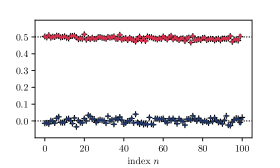
(a) Recurrence coefficients $\overline{\alpha}_{n}$ () and $\overline{\beta}_{n}$ (). Exact arithmetic counterparts shown as pluses () and limiting values shown as dotted lines ().

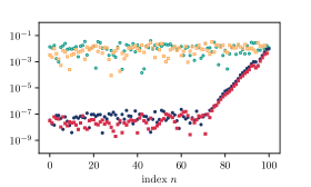
(b) Forward error of recurrence coefficients $|\alpha_{n}-\overline{\alpha}_{n}|$ () and $|\beta_{n}-\overline{\beta}_{n}|$ () and distance to limiting values $|0-\overline{\alpha}_{n}|$ () and $|1/2-\overline{\beta}_{n}|$ ().

Figure 1: Here $(\mathbf{A},\mathbf{b})$ corresponds to a $2000\times 2000$ random matrix, drawn from the Gaussian orthogonal ensemble (see LABEL:sec:wigner), and independent vector. In the large $N$ limit, the VESD of matrices drawn from this ensemble converge to the semicircle distribution on $[-1,1]$ (density $\propto\sqrt{1-x^{2}}$). Therefore the Lanczos coefficients $\alpha_{i}$ and $\beta_{i}$ from the “exact” computation (with reorthogonalization in quadruple precision arithmetic) respectively converge to $1/2$ and $0$; i.e. the Lanczos algorithm exhibits deterministic behavior. In our particular experiment we observe fluctuations on the order of $10^{-2}$ around the limiting values due to finite $N$ effects. Remarkably, the coefficients $\overline{\alpha}_{n}$ and $\overline{\beta}_{n}$ output by the Lanczos algorithm run in single precision floating point arithmetic without reorthogonalization are within the unit roundoff ($\approx 10^{-7}$) of $\alpha_{n}$ and $\beta_{n}$, at least while $n$ is sufficiently small; i.e. the algorithm is forward stable.

The aim of this paper is to provide an intuitive explanation for the observation that the Lanczos algorithm is stable on problems whose VESD are sufficiently regular. More specifically, our approach extends the work of Knizhnerman [knizhnerman_96] to prove the existence of a measure $\mu_{*}$ near to μN whose moments agree with ¯μk through degree $2k-1$, at least when the VESD of $(\mathbf{A},\mathbf{b})$ is sufficiently regular. In fact, under certain regularity conditions, we show there exists a vector $\mathbf{b}_{*}$ near to $\mathbf{b}$ such that Lanczos run on $(\mathbf{A},\mathbf{b}_{*})$ in exact arithmetic for $k$ iterations outputs $\overline{\mathbf{T}}_{k}$. In other words, on a restricted set of inputs, we provide a simpler proof for a stronger version of Greenbaum’s results. We then provide forward stability results by analyzing the orthogonal polynomials of slightly perturbed measures. This shows that, on many large random matrix models, the output of the Lanczos algorithm is nearly deterministic, even when computations are carried out in finite precision arithmetic. Our analysis is accompanied by numerical experiments and several explicit examples.

1.2 Notation

Throughout this work, we use $\Lambda(\mathbf{A})$ to refer to the spectrum of a matrix. For a function $f:U\to\mathbb{C}$ with $S\subseteq U$, we define $\|f\|_{S}:=\sup_{x\in S}|f(x)|$. For a vector $\mathbf{b}$, $\|\mathbf{b}\|$ refers to the Euclidean 2-norm and $\|\mathbf{A}\|$ gives the associated induced operator norm for a matrix $\mathbf{A}$. The $n$-th canonical basis vector, indexed from 0, is $\mathbf{e}_{n}$. The Kolmogorov–Smirnov distance between two measures $\nu_{1}$ and $\nu_{2}$ is $d_{\textup{KS}}(\nu_{1},\nu_{2}):=\sup_{x\in\mathbb{R}}|\nu_{1}((-\infty,x])-\nu_{2}((-\infty,x])$. All measures we consider will be Borel measures. Indeed, all measures will be either fully discrete or have a continuous density.

2 Setup and background

Let $\mu$ be a unit-mass measure with support contained in $[a,b]$. We will refer to $\mu$ as the reference measure, and it will be helpful to think of $\mu$ as near to μN; for instance $\mu=\hyperref@@ii[eqn:VESD]{\color[rgb]{0,0,0}\mu_{N}}$ or $\mu$ being the limiting measure for the VESD of a large random matrix ensemble. In particular, we will typically have $[a,b]\approx[\lambda_{\textup{min}}(\mathbf{A}),\lambda_{\textup{max}}(\mathbf{A})]$. We denote by $\hyperref@@ii[eqn:op]{\color[rgb]{0,0,0}_{n}}=\hyperref@@ii[eqn:op]{\color[rgb]{0,0,0}_{n}}(\cdot\,;\mu)$, $n\geq 0$ the orthonormal polynomials for $\mu$. That is, the $\hyperref@@ii[eqn:op]{\color[rgb]{0,0,0}_{n}}(\cdot\,;\mu)$ satisfy

$$\int\hyperref@@ii[eqn:op]{\color[rgb]{0,0,0}_{n}}(x;\mu)\hyperref@@ii[eqn:op]{\color[rgb]{0,0,0}_{i}}(x;\mu)\mu(\mathrm{d}{x})=\mathds{1}(n=i),$$

where $\mathds{1}(\texttt{true})=1$ and $\mathds{1}(\texttt{false})=0$.

The modified moments of a measure $\nu$ with respect to the orthogonal polynomials of $\mu$ are defined by

$$\hyperref@@ii[eqn:mom]{\color[rgb]{0,0,0}\mathfrak{m}_{n}}(\nu;\mu):=\int\hyperref@@ii[eqn:op]{\color[rgb]{0,0,0}_{n}}(x;\mu)\nu(\mathrm{d}x),\qquad n\geq 0.$$ (2.1)

Clearly $\hyperref@@ii[eqn:mom]{\color[rgb]{0,0,0}\mathfrak{m}_{n}}(\mu;\mu)=\mathds{1}(n=0)$ and $\hyperref@@ii[eqn:mom]{\color[rgb]{0,0,0}\mathfrak{m}_{0}}(\mu;\mu)=\hyperref@@ii[eqn:mom]{\color[rgb]{0,0,0}\mathfrak{m}_{0}}(\hyperref@@ii[eqn:VESD]{\color[rgb]{0,0,0}\mu_{N}};\mu)=\hyperref@@ii[eqn:mom]{\color[rgb]{0,0,0}\mathfrak{m}_{0}}(\hyperref@@ii[eqn:mu_N^k]{\color[rgb]{0,0,0}\mu_{k}};\mu)=\hyperref@@ii[eqn:mom]{\color[rgb]{0,0,0}\mathfrak{m}_{0}}(\hyperref@@ii[eqn:fp_mu_N^k]{\color[rgb]{0,0,0}\overline{\mu}_{k}};\mu)=1$.

As mentioned in the introduction, [knizhnerman_96] shows that the modified moments of μN and ¯μk through degree $2k-1$ are close when $\mu$ is a properly scaled and shifted version of the orthogonality measure for the Chebyshev polynomials of the first kind. A similar statement, with some polynomial losses in $k$, can therefore be expected to hold for any $\mu$ whose orthogonal polynomials have a Chebyshev series representation with reasonable coefficients.

The idea underlying our analysis is to construct a (potentially signed) measure $\mu_{*}$ as a perturbation to the reference measure $\mu$:

$$\mu_{*}(\mathrm{d}{x}):=\left(1+{h}(x)\right)\mu(\mathrm{d}{x}),\quad{h}(x):=\sum_{n=0}^{2k-1}\big{(}\hyperref@@ii[eqn:mom]{\color[rgb]{0,0,0}\mathfrak{m}_{n}}(\hyperref@@ii[eqn:fp_mu_N^k]{\color[rgb]{0,0,0}\overline{\mu}_{k}};\mu)-\hyperref@@ii[eqn:mom]{\color[rgb]{0,0,0}\mathfrak{m}_{n}}(\mu;\mu)\big{)}\hyperref@@ii[eqn:op]{\color[rgb]{0,0,0}_{n}}(x;\mu).$$ (2.2)

This construction ensures $\mu_{*}$ has the same moments as ¯μk through degree $2k-1$ and the same moments as $\mu$ for higher degrees. Indeed, by definition, the pn are orthonormal with respect to $\mu$, so