Dish-TS: A General Paradigm for Alleviating Distribution Shift in
Time Series Forecasting
Abstract
The distribution shift in Time Series Forecasting (TSF), indicating series distribution changes over time, largely hinders the performance of TSF models. Existing works towards distribution shift in time series are mostly limited in the quantification of distribution and, more importantly, overlook the potential shift between lookback and horizon windows. To address above challenges, we systematically summarize the distribution shift in TSF into two categories. Regarding lookback windows as input-space and horizon windows as output-space, there exist (i) intra-space shift, that the distribution within the input-space keeps shifted over time, and (ii) inter-space shift, that the distribution is shifted between input-space and output-space. Then we introduce, Dish-TS, a general neural paradigm for alleviating distribution shift in TSF. Specifically, for better distribution estimation, we propose the coefficient net (Conet), which can be any neural architectures, to map input sequences into learnable distribution coefficients. To relieve intra-space and inter-space shift, we organize Dish-TS as a Dual-Conet framework to separately learn the distribution of input- and output-space, which naturally captures the distribution difference of two spaces. In addition, we introduce a more effective training strategy for intractable Conet learning. Finally, we conduct extensive experiments on several datasets coupled with different state-of-the-art forecasting models. Experimental results show Dish-TS consistently boosts them with a more than 20% average improvement. Code is available at https://github.com/weifantt/Dish-TS.
1 Introduction
Time Series Forecasting (TSF) has been playing an essential role in many applications, such as electricity consumption planning (Akay and Atak 2007), transportation traffic analysis (Ming et al. 2022), weather condition estimation (Abhishek et al. 2012; Han et al. 2021). Following by traditional statistical methods, (e.g., (Holt 1957)), deep learning-based TSF models, (e.g.,, (Salinas et al. 2020; Rangapuram et al. 2018)), have achieved great performance in various areas.
Despite the remarkable success of TSF models, the non-stationarity of time series data has been an under-addressed challenge for accurate forecasting (Hyndman and Athanasopoulos 2018). The non-stationarity, depicting the distribution of series data is shifted over time, can be interpreted as distribution shift in time series (Brockwell and Davis 2009). Such problem results into poor model generalization, thus largely hindering the performance of time series forecasting.
After analyzing numerous series data, we systematically organize distribution shift of TSF into two categories. Considering the lookback windows (‘lookbacks’ for brevity) as input-space of models and horizon windows (‘horizons’ for brevity) as output-space of models111In this paper, we use ‘lookbacks/horizons’, ‘lookback/horizon windows’,‘input/output-space’ interchangeably., there are (i) intra-space shift: time series distribution changes over time, making data within input-space (lookbacks) shifted; (ii) inter-space shift: the distribution is shifted between input-space (lookbacks) and output-space (horizons). Existing works have tried to alleviate distribution shift problem in TSF (Ogasawara et al. 2010; Passalis et al. 2019; Du et al. 2021; Kim et al. 2022). However, most of them exhibit two limitations:
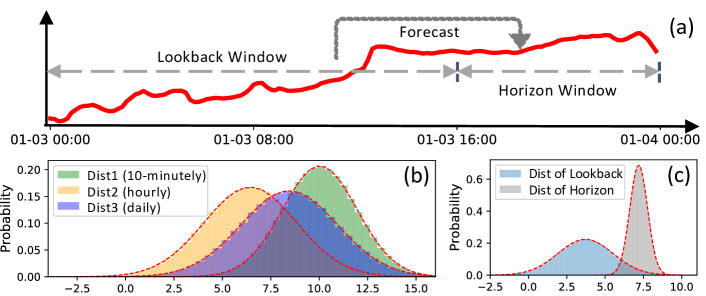
First, the distribution quantification for intra-space in TSF is unreliable. Time series is ideally generated continuously from the true distribution, while the observational data is actually sampled discretely with senors in a certain recording frequency. Existing works always directly normalize or rescale the series (Ogasawara et al. 2010; Passalis et al. 2019; Kim et al. 2022), by quantifying true distribution with fixed statistics (e.g., mean and std.) empirically obtained from observational data, and then normalizing series distribution with these statistics. However, the empirical statistics are unreliable and limited in expressiveness for representing the true distribution behind the data. For example, Figure 1(b) indicates three distributions (depicted by mean and std.) sampled from the same series with different frequencies (i.e., ten-minutely, hourly, daily). Despite coming from the same series, different sampling frequencies provide different statistics, prompting the question: which one best represents the true distribution? Since the recording frequency of time series is determined by sensors, it is difficult to identify what the true distribution is behind the data. Thus, how to properly quantify the distribution, as well as the distribution shift of intra-space, still remains a problem.
Second, the inter-space shift of TSF is neglected. In time series forecasting, considering the input-sequences (lookbacks) and output-sequences (horizons) as two spaces, existing works always assume the input-space and output-space follow the same distribution by default (Ogasawara et al. 2010; Passalis et al. 2019; Du et al. 2021). Though a more recent study, RevIN (Kim et al. 2022), tries to align instances through normalizing the input and denormalizing the output, it still puts a strong assumption that the lookbacks and horizons share the same statistical properties; hence the same distribution. Nonetheless, there is always a variation in distribution between input-space and output-space. As shown in Figure 1(c), the distribution (depicted by mean and std.) between the lookback window and the horizon window exhibits a considerable disparity. The ignorance of inter-space shift overlooks the gap between input- and output-space, thus hindering forecasting performance.
To overcome the above limitations, we propose an effective general neural paradigm, Dish-TS, against Distribution shift in Time Series. Dish-TS is model-agnostic and can be coupled with any deep TSF models. Inspired by (Kim et al. 2022), Dish-TS includes a two-stage process, which normalizes model input before forecasting and denormalizes model output after forecasting. To solve the problem of unreliable distribution quantification, we first propose a coefficient net (Conet) to measure the series distribution. Given any window of series data, Conet maps it into two learnable coefficients: a level coefficient and a scaling coefficient to illustrate series overall scale and fluctuation. In general, Conet can be designed as any neural architectures to conduct any linear/nonlinear mappings, providing sufficient modeling capacity of varied complexities. To relieve the aforementioned intra-space shift and inter-space shift, we organize Dish-TS as a Dual-Conet framework. Specifically, Dual-Conet consists of two separate Conets: (1) BackConet, that produces coefficients to estimate the distribution of input-space (lookbacks), and (2) the HoriConet, that generates coefficients to infer the distribution of output-space (horizons). The Dual-Conet setting captures distinct distributions for input- and output-space respectively, which naturally relieves the inter-space shift.
In addition, Dish-TS is further introduced with an effective prior-knowledge induced training strategy for Conet learning, considering HoriConet needs to infer (or predict) distribution of output-space, which is more intractable due to inter-space shift. Thus, some extra distribution characteristics of output-space is used to provide HoriConet more supervision of prior knowledge. In summary, our contributions are listed:
-
•
We systematically organize distribution shift in time series forecasting as intra-space shift and inter-space shift.
-
•
We propose Dish-TS, a general neural paradigm for alleviating distribution shift in TSF, built upon Dual-Conet with jointly considering intra-space and inter-space shift.
-
•
To implement Dish-TS, we provide a most simple and intuitive instance of Conet design with a prior knowledge-induced training fashion to demonstrate the effectiveness of this paradigm.
-
•
Extensive experiments over various datasets have shown our proposed Dish-TS consistently boost current SOTA models with an average improvement of 28.6% in univariate forecasting and 21.9% in multivariate forecasting.
2 Related Work
Models for Time Series Forecasting.
Time series forecasting (TSF) is a longstanding research topic. At an early stage, researchers have proposed statistical modeling approaches, such as exponential smoothing (Holt 1957) and auto-regressive moving averages (ARMA) (Whittle 1963). Then, more works propose more complicated models: Some researchers adopt a hybrid design (Montero-Manso et al. 2020; Smyl 2020). With the great successes of deep learning, many deep learning models have been developed for time series forecasting (Rangapuram et al. 2018; Salinas et al. 2020; Zia and Razzaq 2020; Cao et al. 2020; Fan et al. 2022). Among them, one most representative one is N-BEATS that (Oreshkin et al. 2020) applies pure fully connected works and achieves superior performance. Transformer (Vaswani et al. 2017) has been also used for series modeling. To improve it, Informer (Zhou et al. 2021) improves in attention computation, memory consumption and inference speed. Recently, Autoformer (Xu et al. 2021) replace attention with auto-correlation to facilitate forecasting.
Distribution Shift in Time Series Forecasting.
Despite of many remarkable models, time series forecasting still suffers from distribution shift considering distribution of real-world series is changing over time (Akay and Atak 2007). To solve this problem, some normalization techniques are proposed: Adaptive Norm (Ogasawara et al. 2010) puts z-score normalization on series by the computed global statistics. Then, DAIN (Passalis et al. 2019) applies nonlinear neural networks to adaptively normalize the series. (Du et al. 2021) proposed Adaptive RNNs to handle the distribution shift in time series. Recently, RevIN (Kim et al. 2022) proposes an instance normalization to reduce series shift. Though DAIN has used simple neural networks for normalization, most works (Ogasawara et al. 2010; Du et al. 2021; Kim et al. 2022) still used static statistics or distance function to describe distribution and normalize series, which is limited in expressiveness. Some other works study time series distribution shift in certain domains such as trading markets (Cao et al. 2022). They hardly consider the inter-space shift between model input-space and output-space.
3 Problem Formulations
Time Series Forecasting.
Let denote the value of a regularly sampled time series at time-step , and the classic time series forecasting formulation is to project historical observations into their subsequent future values , where is the length of lookback windows and is the length of horizon windows. The univariate setting can be easily extended to the multivariate setting. Let stands for distinct time series with the same length , and the multivariate time series forecasting is:
| (1) |
where Gaussian noises exist in the forecasting but dropped for brevity; and are the multivariate lookback window and horizon window respectively; the mapping function can be regarded as a forecasting model parameterized by .
Distribution Shift in Time Series.
As aforementioned, this paper focuses on two kinds of distribution shift in time series. In training forecasting models, one series will be cut into several lookback windows and their corresponding horizon windows . The intra-space shift is defiend as: for any time-step ,
| (2) |
where is a small threshold; is a distance function (e.g., KL divergence); and , standing for the distributions of lookback windows and , are shifted. Note that when most existing works (Ogasawara et al. 2010; Wang et al. 2019; Du et al. 2021; Kim et al. 2022) mention distribution shift in series, they mean our called intra-space shift. In contrast, the inter-space shift is:
| (3) |
where and denotes the distribution of lookback window and horizon window at step , respectively, which is ignored by current TSF models.
4 Dish-TS
In this section, we elaborate on our general neural paradigm, Dish-TS. We start with an overview of this paradigm in Section 4.1. Then, we illustrate the architectures of Dish-TS in Section 4.2. Also, we provide a simple and intuitive instance of Dish-TS in Section 4.3 and introduce a prior knowledge-induced training strategy in Section 4.4, to demonstrate a workable design against the shift in forecasting.
4.1 Overview
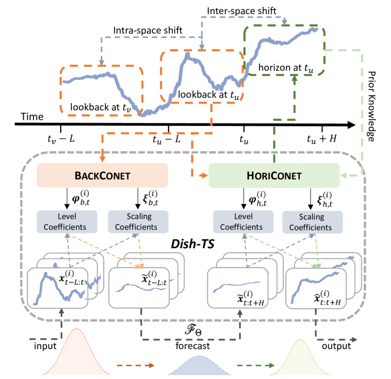
Dish-TS is a simple yet effective, flexible paradigm against distribution shift in time series forecasting. Inspired by (Kim et al. 2022), Dish-TS includes one two-stage process, normalizing before forecasting and denormalizing after forecasting. The paradigm is built upon the coefficient net (Conet), which maps input series into coefficients for distribution measurement. As Figure 2 shows, Dish-TS is organized as a dual-Conet framework, including a BackConet to illustrate input-space (lookbacks) and a HoriConet to illustrate output-space (horizons). Data of lookbacks are transformed by coefficients from BackConet before being taken to any forecasting model ; the output (i.e., forecasting results) are transformed by coefficients from HoriConet to acquire the final predictions. In addition, the HoriConet can be trained in a prior knowledge-induced fashion as a more effective way, especially in long series forecasting.
4.2 Dual-Conet Framework
We introduce Conet and Dual-Conet framework; then we illustrate how forecasting models are integrated into Dual-Conet by a two-stage normalize-denormalize process.
Conet.
Non-stationary time series makes it intractable for accurate predictions. Pilot works (Ogasawara et al. 2010; Du et al. 2021; Kim et al. 2022) measure distribution and its change via statistics (typically mean and std.) or distance function. However, as stated in Section 1, these operations are unreliable quantifications and limited in expressiveness. In this regard, we propose a coefficient net (Conet) for learning better distribution measurement to capture the shift. The general formulation is:
| (4) |
where denotes level coefficient, representing the overall scale of input series in a window ; denotes scaling coefficient, representing fluctuation scale of . In general, Conet could be set as any neural architectures to conduct any linear/nonlinear mappings, which brings sufficient modeling capability and flexibility.
Dual-Conet.
To relieve the aforementioned intra-space shift and inter-space shift in time series, Dish-TS needs to capture the distribution difference among input-space and the difference between input-space and output-space. Inspired by one remarkable model N-BEATS (Oreshkin et al. 2020) that uses ‘backcast’ and ‘forecast’ to conduct backward and forward predictions, we formulate the Dish-TS as a Dual-Conet architecture, including a BackConet for input-space distribution of , and a HoriConet for output-space distribution of . In multivariate forecasting, the two Conets are illustrated as:
| (5) | ||||
where are coefficients for lookbacks, and are coefficients for horizons at time-step , given single -th variate series. Though sharing the same input , the two Conets have distinct targets, where BackConet aims to approximate distribution from input lookback signals, while HoriConet is to infer (or predict) future distribution based on historical observations. This brings additional challenges in training HoriConet, detailed in Section 4.4.
Integrating Dual-Conet into Forecasting.
After acquiring coefficients from Dual-Conet, the coefficients can be integrated into any time series forecasting model to alleviate the two aforementioned shifts through a two-stage normalizing-denormalizing process. Specifically, let represent any forecasting model, the original forecasting process is rewritten as:
| (6) |
where are the final transformed forecasting results after integration with dual conets. Actually, Equation (6) includes a two-stage process with : (i) normalize input lookbacks before forecasting by ; (ii) denormalize model’s direct output after forecasting by . Note that even though the above operations only consider additive and multiplicative transformations, Conet itself could be any complicated linear/nonlinear mappings in the generation of coefficients, which is flexible. Finally, the transformed forecasts are taken to loss optimization.
4.3 A Simple and Intuitive Instance of Conet
Essentially, the flexibility of Dish-TS comes from the specific Conet design, which could be any neural architectures for different modeling capacity. To demonstrate the effectiveness of our framework, we provide a most simple and intuitive instance of Conet design to reduce series shift.
Specifically, given multivariate input , the most intuitive way is to use standard fully connected layers to conduct linear projections. Let stand for two basic learnable vectors of layer of BackConet and HoriConet respectively. Here we consider for simplicity, and then the projection is:
| (7) |
where the level coefficients and are respectively from BackConet and HoriConet to represent the overall scale of input and output ; here denotes a leaky ReLU non-linearity (Maas et al. 2013) is utilized instead of original ReLU that ignores negative data and thus causes information loss. Also, we aim to let scaling coefficients represent the fluctuation for series. Inspired by the calculation of standard deviation where is variable and is mean, we propose the following operation to get scaling coefficients:
| (8) |
where scaling coefficients can actually be seen as the average deviation of with regard to and . The equation (8) is also simple, intuitive and easy to compute, without introducing extra parameters to optimize.
4.4 Prior Knowledge-Induced Training Strategy
As aforementioned, BackConet estimates distribution of input-space , while HoriConet needs to infer distribution of output-space , which is more intractable because of the gap between input- and output-space. The gap is even larger with the increase of horizon length.
To solve this problem, we aim to pour some prior knowledge (i.e., mean of horizons) as soft targets in Dish-TS to assist the learning of HoriConet to generate coefficients . Even though the statistic mean of horizons cannot fully reflect the distribution, it can still demonstrate characteristics of output-space, as discussed in Section 1. Thus, along the line of equation (6), the classic mean square error can be given by , where is the batch size, is randomly-sampled time points to compose batches, and is number of series. With prior knowledge, we rewrite the final optimization loss as:
| (9) |
where the left item is mean square error; the right item is the learning guidance of prior knowledge; is to control weight of prior guidance; is the level coefficients of HoriConet to softly optimize.
| Method | Informer | +Dish-TS | Autoformer | +Dish-TS | N-BEATS | +Dish-TS | |||||||
|---|---|---|---|---|---|---|---|---|---|---|---|---|---|
| Metric | MSE | MAE | MSE | MAE | MSE | MAE | MSE | MAE | MSE | MAE | MSE | MAE | |
| Electricity | 24 | 4.394 | 4.897 | 1.116 | 2.413 | 1.616 | 3.138 | 1.535 | 2.942 | 1.259 | 2.572 | 1.205 | 2.536 |
| 48 | 4.405 | 4.904 | 1.256 | 2.581 | 2.291 | 3.772 | 1.783 | 3.199 | 1.311 | 2.696 | 1.286 | 2.629 | |
| 96 | 3.933 | 4.675 | 1.060 | 2.354 | 2.281 | 3.726 | 1.330 | 2.706 | 1.271 | 2.625 | 1.129 | 2.447 | |
| 168 | 4.083 | 4.747 | 1.015 | 2.301 | 2.072 | 3.502 | 1.162 | 2.413 | 1.520 | 2.879 | 0.985 | 2.261 | |
| 336 | 4.292 | 4.848 | 2.893 | 4.364 | 2.112 | 3.481 | 1.387 | 2.722 | 1.747 | 3.107 | 1.497 | 2.852 | |
| ETTh1 | 24 | 0.427 | 1.536 | 0.339 | 1.343 | 0.420 | 1.505 | 0.344 | 1.350 | 0.406 | 1.479 | 0.320 | 1.279 |
| 48 | 0.855 | 2.272 | 0.570 | 1.824 | 0.767 | 2.172 | 0.588 | 1.885 | 0.598 | 1.841 | 0.569 | 1.815 | |
| 96 | 0.930 | 2.328 | 0.840 | 2.258 | 1.100 | 2.669 | 0.872 | 2.340 | 0.827 | 2.254 | 0.785 | 2.168 | |
| 168 | 0.964 | 2.567 | 0.911 | 2.448 | 1.098 | 2.659 | 0.959 | 2.488 | 1.052 | 2.617 | 0.908 | 2.399 | |
| 336 | 1.146 | 2.829 | 0.993 | 2.520 | 1.230 | 2.796 | 0.936 | 2.454 | 1.117 | 2.639 | 1.011 | 2.550 | |
| ETTm2 | 24 | 1.328 | 2.525 | 0.760 | 1.686 | 1.718 | 2.976 | 0.762 | 1.851 | 0.867 | 1.804 | 0.600 | 1.479 |
| 48 | 1.488 | 2.649 | 1.070 | 2.117 | 3.061 | 4.259 | 1.847 | 3.082 | 1.290 | 2.374 | 1.145 | 2.160 | |
| 96 | 2.952 | 4.324 | 1.631 | 2.771 | 3.113 | 4.309 | 2.385 | 3.648 | 1.707 | 2.922 | 1.605 | 2.747 | |
| 168 | 5.114 | 5.832 | 2.754 | 3.841 | 4.167 | 4.959 | 3.413 | 4.452 | 2.428 | 3.603 | 2.380 | 3.579 | |
| 336 | 5.958 | 6.490 | 4.284 | 5.096 | 5.753 | 5.993 | 4.449 | 5.213 | 3.974 | 4.815 | 3.568 | 4.582 | |
| Weather | 24 | 3.632 | 1.381 | 0.725 | 0.584 | 1.082 | 0.775 | 0.800 | 0.622 | 0.570 | 0.486 | 0.567 | 0.480 |
| 48 | 5.933 | 1.856 | 1.251 | 0.798 | 1.617 | 0.968 | 1.317 | 0.845 | 1.272 | 0.825 | 1.178 | 0.776 | |
| 96 | 6.895 | 2.071 | 1.898 | 1.022 | 1.901 | 1.034 | 1.824 | 1.005 | 1.898 | 0.995 | 1.783 | 0.994 | |
| 168 | 6.786 | 2.045 | 1.932 | 1.042 | 1.970 | 1.046 | 1.847 | 1.008 | 2.571 | 1.210 | 1.848 | 1.024 | |
| 336 | 7.393 | 2.175 | 2.237 | 1.099 | 2.190 | 1.100 | 2.015 | 1.061 | 3.624 | 1.486 | 2.447 | 1.117 | |
-
•
Results of Illness dataset are included Appendix B.1, due to space limit.
5 Experiment
5.1 Experimental Setup
Datasets.
We conduct our experiments on five real-world datasets: (i) Electricity dataset collects the electricity consumption (Kwh) of 321 clients. (ii) ETT dataset includes data of electricity transformers temperatures. We select ETTh1 dataset (hourly) and ETTm2 dataset (15-minutely). (iii) Weather dataset records 21 meteorological features every ten minutes. (iv) Illness dataset includes weekly-recorded influenza-like illness patients data. We mainly follow (Zhou et al. 2021) and (Xu et al. 2021) to preprocess and split data. More details are in Appendix A.1
Evaluation.
To directly reflect distribution shift in time series, all the experiments are conducted on original data without data normalization or scaling. We evaluate time series forecasting performance on the mean squared error (MSE) and mean absolute error (MAE). Note that our evaluations are on original data; thus the reported metrics are scaled for readability. More evaluation details are in Appendix A.2.
Implementation.
All the experiments are implemented with PyTorch (Paszke et al. 2019) on an NVIDIA RTX 3090 24GB GPU. In training, all the models are trained using L2 loss and Adam (Kingma and Ba 2014) optimizer with learning rate of [1e-4, 1e-3]. We repeat three times for each experiment and report average performance. We let lookback/horizon windows have the same length, gradually prolonged from 24 to 336 except for illness dataset that has length limitation. We have also discussed larger lookback length , larger horizon length , and prior guidance rate . Implementation details are included in Appendix A.3.
Baselines.
As aforementioned, our Dish-TS is a general neural framework that can be integrated into any deep time series forecasting models for end-to-end training. To verify the effectiveness, we couple our paradigm with three state-of-the-art backbone models, Informer (Zhou et al. 2021), Autoformer (Xu et al. 2021) and N-BEATS (Oreshkin et al. 2020). More baseline details are in Appendix A.4.
| Method | Informer | +Dish-TS | Autoformer | +Dish-TS | N-BEATS | +Dish-TS | |||||||
|---|---|---|---|---|---|---|---|---|---|---|---|---|---|
| Metric | MSE | MAE | MSE | MAE | MSE | MAE | MSE | MAE | MSE | MAE | MSE | MAE | |
| Electricity | 24 | 0.482 | 0.575 | 0.036 | 0.249 | 0.082 | 0.420 | 0.040 | 0.247 | 0.041 | 0.281 | 0.032 | 0.241 |
| 48 | 0.969 | 1.002 | 0.056 | 0.289 | 0.125 | 0.450 | 0.051 | 0.278 | 0.043 | 0.275 | 0.041 | 0.265 | |
| 96 | 1.070 | 1.046 | 0.084 | 0.325 | 0.363 | 0.642 | 0.064 | 0.285 | 0.067 | 0.324 | 0.058 | 0.286 | |
| 168 | 0.960 | 1.013 | 0.088 | 0.335 | 0.585 | 0.835 | 0.080 | 0.319 | 0.078 | 0.347 | 0.074 | 0.294 | |
| 336 | 1.113 | 1.058 | 0.153 | 0.400 | 0.569 | 0.766 | 0.104 | 0.357 | 0.108 | 0.383 | 0.108 | 0.355 | |
| ETTh1 | 24 | 0.988 | 1.794 | 0.876 | 1.633 | 1.451 | 2.100 | 1.019 | 1.744 | 0.797 | 1.531 | 0.790 | 1.501 |
| 48 | 1.318 | 2.127 | 1.073 | 1.846 | 1.456 | 2.161 | 1.240 | 1.966 | 0.913 | 1.696 | 0.907 | 1.657 | |
| 96 | 2.333 | 2.965 | 1.185 | 2.011 | 1.371 | 2.173 | 1.199 | 1.982 | 1.057 | 1.875 | 0.975 | 1.793 | |
| 168 | 2.778 | 3.234 | 1.273 | 2.085 | 1.267 | 2.146 | 1.148 | 1.991 | 1.038 | 1.893 | 0.994 | 1.858 | |
| 336 | 2.825 | 3.335 | 1.779 | 2.586 | 1.334 | 2.333 | 1.147 | 2.062 | 1.128 | 2.020 | 1.055 | 1.976 | |
| ETTm2 | 24 | 1.352 | 2.443 | 0.608 | 1.594 | 0.834 | 1.882 | 0.676 | 1.701 | 0.643 | 1.609 | 0.634 | 1.587 |
| 48 | 1.781 | 2.973 | 0.736 | 1.767 | 1.165 | 2.269 | 0.823 | 1.903 | 0.808 | 1.829 | 0.785 | 1.793 | |
| 96 | 1.936 | 3.017 | 0.877 | 1.946 | 1.165 | 2.237 | 0.929 | 2.021 | 0.953 | 2.017 | 0.860 | 1.904 | |
| 168 | 2.822 | 3.656 | 1.213 | 2.273 | 1.404 | 2.423 | 1.308 | 2.367 | 1.094 | 2.143 | 1.087 | 2.156 | |
| 336 | 2.778 | 3.638 | 1.620 | 2.637 | 1.795 | 2.739 | 1.603 | 2.624 | 1.498 | 2.543 | 1.448 | 2.522 | |
| Weather | 24 | 3.552 | 2.120 | 2.224 | 1.100 | 4.485 | 2.313 | 2.481 | 1.163 | 2.557 | 1.454 | 2.267 | 1.093 |
| 48 | 4.206 | 2.231 | 3.610 | 1.644 | 6.581 | 2.815 | 4.299 | 1.781 | 5.527 | 2.393 | 4.783 | 1.802 | |
| 96 | 3.064 | 2.042 | 2.507 | 1.457 | 5.812 | 2.569 | 3.280 | 1.806 | 2.539 | 1.566 | 2.280 | 1.367 | |
| 168 | 2.713 | 2.106 | 2.184 | 1.450 | 4.053 | 2.188 | 3.309 | 1.950 | 2.160 | 1.604 | 1.885 | 1.309 | |
| 336 | 3.472 | 2.567 | 2.238 | 1.611 | 3.910 | 2.111 | 3.314 | 1.982 | 2.043 | 1.551 | 1.757 | 1.366 | |
-
•
means N-BEATS is re-implemented for multivariate time series forecasting; see Appendix A.4 for more details.
| Datasets | Electiricity | ETTh1 | ETTm2 | Weather | ||||||||
|---|---|---|---|---|---|---|---|---|---|---|---|---|
| Length | 24 | 168 | 336 | 24 | 168 | 336 | 24 | 168 | 336 | 24 | 168 | 336 |
| RevIN | 0.044 | 0.091 | 0.109 | 1.245 | 1.462 | 1.920 | 0.794 | 1.501 | 1.827 | 3.523 | 3.658 | 3.501 |
| Dish-TS | 0.039 | 0.076 | 0.086 | 1.018 | 1.148 | 1.222 | 0.651 | 1.325 | 1.599 | 2.481 | 3.283 | 3.232 |
| Improve | 11.3% | 15.3% | 21.1% | 18.1% | 21.4% | 36.3% | 17.7% | 11.7% | 12.3% | 29.6% | 10.7% | 7.7% |
5.2 Overall Performance
Univariate time series forecasting. Table 1 demonstrates the overall univariate time series forecasting performance of three state-of-the-art backbones and their Dish-TS equipped versions, where we can easily observe that Dish-TS helps all the backbones achieve much better performance. The most right column of Table 1 shows the average improvement of Dish-TS over baseline models under different circumstances. We can see that Dish-TS can achieve a MSE improvement more than 20% in most cases, up to 50% in some cases. Notably, Informer usually performs worse but can be improved significantly with Dish-TS.
Multivariate time series forecasting. Table 2 demonstrates the overall multivariate time series forecasting performance across four datasets and the results and analysis for Illness dataset are in Appendix B.1. Still, we notice Dish-TS can also improve significantly in the task of multivariate forecasting compared with three backbones. We find out a stable improvement (from 10% to 30%) on ETTh1, ETTm2 and Weather datasets when coupled with Dish-TS. Interestingly, we notice the both original Informer and Autoformer can hardly converge well in Electricity original data. With Dish-TS, the data distribution is normalized for better forecasting.
5.3 Comparison with Normalization Methods
In this section, we further compare performance with the state-of-the-art normalization technique, RevIN (Kim et al. 2022), that handles distribution shift in time series forecasting. Here we don’t consider AdaRNN (Du et al. 2021) because it is not compatible for fair comparisons. Table 3 shows the comparison results in multivariate time series forecasting. We can easily observe though RevIN actually improves performance of vanilla backbone (Autoformer) to some degree, Dish-TS can still achieve more than 10% improvement on average compared with RevIN. A potential reason for this significant improvement of such a simple Conet design is the consideration towards both intra-space shift and inter-space shift.
| Horizon | 336 | 420 | 540 | 600 | 720 |
|---|---|---|---|---|---|
| Electricity | 1.7429 | 1.7859 | 1.7720 | 1.6140 | 1.6023 |
| +Dish-TS | 1.3361 | 1.4507 | 1.4107 | 1.4340 | 1.4785 |
| ETTh1 | 1.0468 | 1.2688 | 1.1696 | 1.3281 | 1.4270 |
| +Dish-TS | 0.9699 | 1.0864 | 1.1361 | 1.1852 | 1.1913 |

5.4 Parameters and Model Analysis
Horizon Analysis.
We aim to discuss the influence of larger horizons (known as long time series forecasting (Zhou et al. 2021)) on the model performance. Interestingly, from Table 4, we find out backbone (N-BEATS) performs even better in Electricity as horizon becomes larger while on other datasets like ETTh1 larger horizons introduce more difficulty in forecasting. However, Dish-TS can still achieve better performance in different settings. Performance on Dish-TS is slowly worse with horizon’s increasing. An intuitive reason is larger horizons include more distribution changes and thus need more complicated modeling.
| Lookback | 48 | 96 | 144 | 192 | 240 |
|---|---|---|---|---|---|
| Electricity | 1.3026 | 1.3673 | 1.2794 | 1.2686 | 0.9494 |
| +Dish-TS | 1.2862 | 0.9682 | 0.7309 | 0.7156 | 0.7605 |
| ETTh1 | 0.5979 | 0.5745 | 0.5459 | 0.5638 | 0.6309 |
| +Dish-TS | 0.5708 | 0.5451 | 0.5202 | 0.5307 | 0.5234 |
Lookback Analysis.
We analyze the influence of lookback length on the model performance. As Table 5 shows, we notice Dish-TS achieves on Electricity and when lookback increases from 48 to 144. This signifies in many cases larger lookback windows bring more historical information to infer the future distribution, thus boosting the prediction performance.
Prior Guidance Rate.
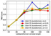
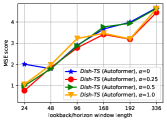
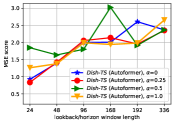
We study the impact of prior guidance on model performance. Figure 3 shows the performance comparison with different guidance weight in Equation (9). From the table, we observe when lookback/horizon is small, the performance gap among different s is less obvious. However, when length is larger (than 168), the prediction error of (no guidance) increases quickly, while other settings achieve less errors. This shows prior knowledge can help better HoriConet learning, especially in the settings of long time series forecasting.
| Model | Dish-TS (Autoformer) | Dish-TS (N-BEATS) | |||||
|---|---|---|---|---|---|---|---|
| Initilize | avg | norm | uniform | avg | norm | uniform | |
| ETTh1 | 24 | 3.439 | 3.658 | 3.532 | 3.196 | 3.230 | 3.292 |
| 96 | 8.794 | 9.381 | 8.774 | 7.878 | 8.067 | 7.851 | |
| 168 | 9.878 | 9.725 | 9.589 | 9.783 | 9.250 | 9.080 | |
| Weather | 24 | 1.579 | 0.835 | 0.799 | 0.650 | 0.579 | 0.566 |
| 96 | 2.127 | 2.056 | 1.823 | 1.915 | 1.814 | 1.782 | |
| 168 | 2.139 | 3.140 | 1.847 | 1.848 | 2.323 | 2.054 | |
Conet Initialization.
We aim to study the impact of Conet initialization on model performance. As mentioned in Section 4.3, we create two learnable vectors for Conets. We consider three strategies to initialize : (i) : with scalar ones; (ii) : with standard normal distribution; (iii) : with random distribution between 0 and 1. From Table 6, we observe three strategies perform similarly in most cases, showing stable performance. We also notice and initialization performs better than , which signifies Dish-TS and the hidden distribution may be better learned when not using initialization.
Computational Consumption.
We record the extra memory consumption of Dish-TS. As shown in Appendix B.3, our simple instance of Dish-TS (referred in Section 4.3) only causes extra 4MiB (or less) memory consumption, which can be ignored in real-world applications.
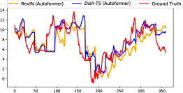
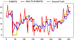
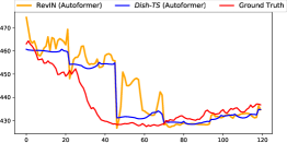
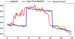
Visualizations.
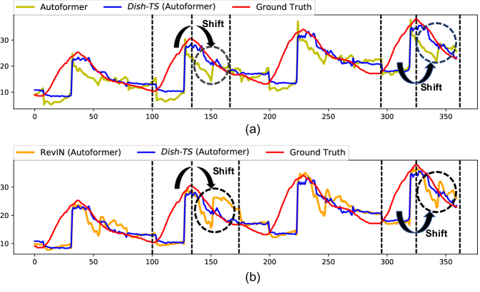
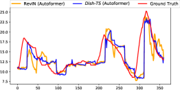
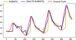
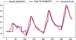
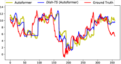
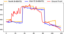
We compare predictions of base model and Dish-TS in Figure 4(a), predictions of RevIN (Kim et al. 2022) and Dish-TS in Figure 4(b). We easily observe when series trend largely changes (could be regarded as the distribution largely changes), both backbone model (Autoformer) and RevIN cannot acquire accurate predictions (in black circles). In contrast, our Dish-TS can still make correct forecasting. We show more visualizations in Appendix B.4.
6 Conclusion Remarks
In this paper, we systematically summarize the distribution shift in time series forecasting as intra-space shift and inter-space shift. We propose a general paradigm, Dish-TS to better alleviate the two shift. To demonstrate the effectiveness, we provide a most simple and intuitive instance of Dish-TS along with a prior knowledge-induced training strategy, to couple with state-of-the-art models for better forecasting. We conduct extensive experiments on several datasets and the results demonstrate a very significant improvement over backbone models. We hope this general paradigm together with such an effective instance of Dish-TS design can facilitate more future research on distribution shift in time series.
| Dataset | Electricity | ETTh1 | ETTm2 | Weather | Illness | |||||
|---|---|---|---|---|---|---|---|---|---|---|
| Metric | MSE | MAE | MSE | MAE | MSE | MAE | MSE | MAE | MSE | MAE |
| Uni-variate | ||||||||||
| Multi-variate | ||||||||||
Appendix A More Experimental Details
A.1 More Dataset Details
We conduct our experiments on the following five real-world datasets:
-
•
Electricity222https://archive.ics.uci.edu/ml/datasets/ElectricityLoadDiagrams20112014 dataset collects the electricity consumption (Kwh) of 321 clients, and raw data is pre-processed following (Xu et al. 2021).
-
•
ETT333https://github.com/zhouhaoyi/ETDataset datasets contain the data of electricity transformers temperatures of 2-years data collected from two counties in China. The experiments are on two granularity versions of raw data, namely ETTh1 dataset (1-hour-level) and ETTm2 dataset (15-minutes-level).
-
•
Weather444https://www.bgc-jena.mpg.de/wetter/ dataset is recorded in ten-minute level in 2020, which contains 21 meteorological indicators, such as air humidity, etc.
-
•
Illness555https://gis.cdc.gov/grasp/fluview/fluportaldashboard.html dataset has the weekly recorded influenza-like illness (ILI) patients data from Centers for Disease Control and Prevention of the United States between 2002 and 2021, which describes the ratio of patients seen with and the total number of the patients.
For data split, we follow (Zhou et al. 2021) and split data into train/validation/test set by the ratio 6:2:2 towards ETTm1 and ETTh2 datasets. We follow (Xu et al. 2021) to preprocess data and split data by the ratio of 7:1:2 in Electricity, Weather and Illness datasets.
A.2 More Evaluation Details
To directly reflects the shift in time series, all experiments and evaluations are conducted on original data without any data normalization or data scaling, which is different from experimental settings of (Zhou et al. 2021; Xu et al. 2021) which use z-score normalization to process data before training and evaluation.
In evaluation, we evaluate the time series forecasting performances on the mean squared error (MSE) and mean absolute error (MAE). Note that our experiments and evaluations are on original data; thus the reported metrics are scaled for readability. Specifically, in univariate forecasting, MSE and MAE is scaled by on Electricity, on Weather, on Illness, and on all ETT datasets.In multivariate forecasting, MSE and MAE is scaled by on Electricity, on Weather, on Illness, and on ETT datasets. This setting is summarized in Table 7.
| Method | Informer | +Dish-TS | Autoformer | +Dish-TS | N-BEATS | +Dish-TS | |||||||
|---|---|---|---|---|---|---|---|---|---|---|---|---|---|
| Metric | MSE | MAE | MSE | MAE | MSE | MAE | MSE | MAE | MSE | MAE | MSE | MAE | |
| Illness | 24 | 1.405 | 1.159 | 0.050 | 0.154 | 0.066 | 0.208 | 0.065 | 0.199 | 0.048 | 0.167 | 0.046 | 0.166 |
| 36 | 1.390 | 1.154 | 0.036 | 0.149 | 0.050 | 0.183 | 0.040 | 0.158 | 0.062 | 0.191 | 0.040 | 0.155 | |
| 48 | 1.383 | 1.151 | 0.040 | 0.169 | 0.064 | 0.210 | 0.054 | 0.189 | 0.053 | 0.174 | 0.035 | 0.152 | |
| 60 | 1.398 | 1.158 | 0.038 | 0.165 | 0.075 | 0.229 | 0.055 | 0.195 | 0.071 | 0.219 | 0.039 | 0.163 | |
| 96 | 1.404 | 1.163 | 0.090 | 0.258 | 0.148 | 0.336 | 0.081 | 0.242 | 0.067 | 0.205 | 0.056 | 0.201 | |
| Method | Informer | +Dish-TS | Autoformer | +Dish-TS | N-BEATS | +Dish-TS | |||||||
|---|---|---|---|---|---|---|---|---|---|---|---|---|---|
| Metric | MSE | MAE | MSE | MAE | MSE | MAE | MSE | MAE | MSE | MAE | MSE | MAE | |
| Illness | 24 | 2.009 | 1.718 | 0.062 | 0.248 | 0.096 | 0.349 | 0.091 | 0.308 | 0.065 | 0.256 | 0.062 | 0.248 |
| 36 | 1.988 | 1.710 | 0.052 | 0.244 | 0.078 | 0.328 | 0.057 | 0.252 | 0.057 | 0.260 | 0.057 | 0.257 | |
| 48 | 1.979 | 1.708 | 0.053 | 0.259 | 0.079 | 0.325 | 0.069 | 0.297 | 0.054 | 0.245 | 0.053 | 0.240 | |
| 60 | 1.999 | 1.720 | 0.060 | 0.280 | 0.107 | 0.377 | 0.080 | 0.324 | 0.050 | 0.235 | 0.048 | 0.235 | |
| 96 | 2.009 | 1.729 | 0.130 | 0.410 | 0.203 | 0.514 | 0.107 | 0.369 | 0.086 | 0.334 | 0.077 | 0.311 | |
A.3 More Implementation Details
In the main experiments of univariate/multivariate time series forecasting, we let the lookback window and the horizon window have the same length, where we gradually prolong the length as to accommodate short-term/long-term settings. For illness dataset, the length is set as due to the length limitation of the dataset. The length of horizon is further extended to 720 when fixed the length of lookback as 96 in model analysis experiments, in order to study the long time series forecasting (LSTF) problems (Zhou et al. 2021).
We train all the models using L2 loss and Adam (Kingma and Ba 2014) optimizer with learning rate of [1e-4, 1e-3]. We repeat three times for each experiment and report average performance. The batchsize is set as 256 for Informer, 128 for Autoformer and 1024 for N-BEATS, apart from that in Electricity dataset, the batchsize is set 64 for Autoformer and Informer. We set the early stop with 7 steps. We let equal to 1 to reduce extra consumption as much as possible. The rate of prior knowledge guidance is traversed from 0 to 1. All the experiments are implemented with PyTorch (Paszke et al. 2019) on single NVIDIA RTX 3090 24GB GPU.
A.4 More Baseline Details.
As aforementioned, our Dish-TS is a general framework that can be integrated into any deep time series forecasting models. To verify the effectiveness, we couple our dual-conet framework with three state-of-the-art models, Informer (Zhou et al. 2021), Autoformer (Xu et al. 2021) and N-BEATS (Oreshkin et al. 2020). In the main results, we compare the performance of the above three models and their Dish-TS coupled versions. Mainly we reproduce the model by following their open source github links.
The detailed implementation details are as follows:
-
•
Informer. We use the official open-source code of (Zhou et al. 2021)666https://github.com/zhouhaoyi/Informer2020. For the hyper-parameter settings, we set them same as original paper, including number of heads, dimension of PropSparse attntion, dimension of feed-forward layer, etc. In addition, we remove time embeddings of Informer to align with N-BEATS.
-
•
Autoformer. We use the official open-source code of (Xu et al. 2021)777https://github.com/thuml/Autoformer. For hyper-parameter settings, we follow the original settings including moving average of Auto-correlation layer, dimension of Auto-Correlation layer, etc. We also remove time embeddings to align with N-BEATS.
-
•
N-BEATS. We take the notable reproduced codes of N-BEATS888https://github.com/ElementAI/N-BEATS. We carefully choose the parameter settings of N-BEATS and set number of stacks as 3, number of layers as 10 with 256 as layer size. Note that N-BEATS is an univariate time series forecasting model. To align with the input and output of Informer/Autoformer, we transform the multivariate lookback windows from dimension to , where is batchsize, is lookback length and is number of series. The horizon windows adopt the same strategy. In the mean time, for multivatiate forecasting on different datasets, we set equals to to avoid very large batch size that influences training.
To compare fairly, we compare baselines and their Dish-TS-coupled versions under the same experimental settings with all same hyperparameters.
Appendix B More Experimental Results
B.1 More Results of Overall Performance
In this section, we include more experimental results of overall performance on Illness datasets.
Univariate Time Series Forecasting. Table 8 shows the univariate time series forecasting performance on Illness. We notice that Informer still performs very badly, while Dish-TS can still achieve better performances in most cases. Also, the improvement is more obvious when the lookback/horizon length is larger except for few cases, which shows our superiority in forecasting.
Multivariate Time Series Forecasting. Table 9 shows the multivariate time series forecasting performance on Illness dataset. Firstly, we still observe Informer cannot converge well so we don’t discuss it more. From the backbone N-BEATS, we observe the improvement is not that significant except when length is 96. However, From the backbone Autoformer, we find the average improvement is very significant, especially when length is 96, the improvement is , about . These observations also show that our Dish-TS can handle the situations when lookback/horizon grows larger.
| Datasets | Electiricity | ETTh1 | ETTm2 | Weather | ||||||||
|---|---|---|---|---|---|---|---|---|---|---|---|---|
| Length | 24 | 96 | 168 | 24 | 96 | 168 | 24 | 96 | 168 | 24 | 96 | 168 |
| RevIN | 1.606 | 1.769 | 1.470 | 0.435 | 1.088 | 1.066 | 1.193 | 3.059 | 4.068 | 0.987 | 2.131 | 2.113 |
| Dish-TS | 1.535 | 1.330 | 1.162 | 0.344 | 0.872 | 0.959 | 0.762 | 2.385 | 3.413 | 0.800 | 1.824 | 1.847 |
| Improve | 4.4% | 24.8% | 21.0% | 20.9% | 19.8% | 10.1% | 36.2% | 22.0% | 16.1% | 18.9% | 14.4% | 12.5% |
| Model | Autoformer | +Dish-TS | N-BEATS | +Dish-TS |
|---|---|---|---|---|
| ETTh1 | 6781MiB | 6783MiB | 2503MiB | 2507MiB |
| Weather | 9085MiB | 9089MiB | 2495MiB | 2497MiB |
B.2 Comparison with Normalization Techniques
In this section, as shown in Table 10,we further report the performance comparison of the state-of-the-art normalization technique RevIN (Kim et al. 2022)) in univariate time series forecasting.
From the table, we can still easily observe Dish-TS can still perform better than RevIN. The improvement towards RevIN is more than 10% mostly, up to 36% in one case. Though RevIN can actually help backbone models improve to some extent, our Dish-TS can still achieve better performances compared with RevIN, showing much effectiveness. A potential reason for the improvement towards RevIN comes from the considerations towards inter-space shift, which is ignored by RevIN. Based on this result, we notice that not only in multivariate forecasting but also in univariate forecasting, our Dish-TS can perform better than existing works, which demonstrates the superiority of our proposed Dish-TS.
B.3 Computational Consumption
B.4 More Visualization Cases
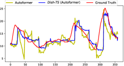
We show more visualization cases on ETTh1, ETTm2, and Weather dataset: Figure 6 and Figure 7 shows the forecastings of backbone, RevIN, Dish-TS on ETTm2 dataset, taking Autoformer and N-BEATS as backbones. Figure 8 and Figure 9 demonstrate the forecastings of backbone, RevIN, Dish-TS on ETTh1 dataset with Autoformer and N-BEATS respectively. Figure 10 and Figure 11 demonstrate the forecastings of backbone, RevIN, Dish-TS on Weather dataset with Autoformer and N-BEATS respectively.
Interestingly, we can consistently notice that when series trend changes dramatically (sudden rise or drop), our Dish-TS can help backbone models to acquire more accurate forecasting. This signifies that when series distribution largely changes, Dish-TS can be better solution for time series forecasting against distribution shift. These visualizations show that Dish-TS forecasts well in shifted time series.
B.5 Visualization of Quantified Distribution
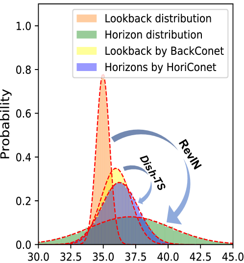
We further visualize the distribution quantification in Figure 5. Specifically, we first randomly sample 100 lookback windows and 100 horizon windows from test data of ETTm2 dataset. We firstly visualize the the distribution of lookback (in orange of Figure 5) and horizon (in green of Figure 5), depicted by mean and std. for the sampled data. Essentially, the RevIN (Kim et al. 2022) is to use statistical of lookback distribution to infer the horizon distribution. Thus, the backbone of RevIN needs to go through the transformation of (the blue arrow from orange to green in Figure 5). We also show the lookback and horizon distribution processed by BackConet and HoriConet of Dish-TS, in yellow and in blue of Figure 5 respectively. Accordingly, we notice the backbone model with Dish-TS only needs to conduct mappings (forecasting) of small blue arrow in Figure 5). This quantification results show that Dish-TS itself models distribution shift and thus leaves less burden to backbone models, which is also an intuitive reason of our significant improvement to RevIN.
Acknowledgements
This research was partially supported by the National Science Foundation (NSF) via the grant numbers: 2040950, 2006889, 2045567.


References
- Abhishek et al. (2012) Abhishek, K.; Singh, M.; Ghosh, S.; and Anand, A. 2012. Weather forecasting model using artificial neural network. Procedia Technology, 4: 311–318.
- Akay and Atak (2007) Akay, D.; and Atak, M. 2007. Grey prediction with rolling mechanism for electricity demand forecasting of Turkey. energy, 32(9): 1670–1675.
- Brockwell and Davis (2009) Brockwell, P. J.; and Davis, R. A. 2009. Time series: theory and methods. Springer science & business media.
- Cao et al. (2022) Cao, D.; El-Laham, Y.; Trinh, L.; Vyetrenko, S.; and Liu, Y. 2022. A Synthetic Limit Order Book Dataset for Benchmarking Forecasting Algorithms under Distributional Shift. In NeurIPS 2022 Workshop on Distribution Shifts: Connecting Methods and Applications.
- Cao et al. (2020) Cao, D.; Wang, Y.; Duan, J.; Zhang, C.; Zhu, X.; Huang, C.; Tong, Y.; Xu, B.; Bai, J.; Tong, J.; et al. 2020. Spectral temporal graph neural network for multivariate time-series forecasting. Advances in neural information processing systems, 33: 17766–17778.
- Du et al. (2021) Du, Y.; Wang, J.; Feng, W.; Pan, S.; Qin, T.; Xu, R.; and Wang, C. 2021. Adarnn: Adaptive learning and forecasting of time series. In Proceedings of the 30th ACM International Conference on Information & Knowledge Management, 402–411.
- Fan et al. (2022) Fan, W.; Zheng, S.; Yi, X.; Cao, W.; Fu, Y.; Bian, J.; and Liu, T.-Y. 2022. DEPTS: Deep Expansion Learning for Periodic Time Series Forecasting. In International Conference on Learning Representations.
- Han et al. (2021) Han, J.; Liu, H.; Zhu, H.; Xiong, H.; and Dou, D. 2021. Joint Air Quality and Weather Prediction Based on Multi-Adversarial Spatiotemporal Networks. In Proceedings of the 35th AAAI Conference on Artificial Intelligence.
- Holt (1957) Holt, C. C. 1957. Forecasting trends and seasonal by exponentially weighted moving averages. ONR Memorandum, 52(2).
- Hyndman and Athanasopoulos (2018) Hyndman, R. J.; and Athanasopoulos, G. 2018. Forecasting: principles and practice. OTexts.
- Kim et al. (2022) Kim, T.; Kim, J.; Tae, Y.; Park, C.; Choi, J.-H.; and Choo, J. 2022. Reversible instance normalization for accurate time-series forecasting against distribution shift. In International Conference on Learning Representations.
- Kingma and Ba (2014) Kingma, D. P.; and Ba, J. 2014. Adam: A method for stochastic optimization. arXiv preprint arXiv:1412.6980.
- Maas et al. (2013) Maas, A. L.; Hannun, A. Y.; Ng, A. Y.; et al. 2013. Rectifier nonlinearities improve neural network acoustic models. In Proc. icml, volume 30, 3. Citeseer.
- Ming et al. (2022) Ming, J.; Zhang, L.; Fan, W.; Zhang, W.; Mei, Y.; Ling, W.; and Xiong, H. 2022. Multi-Graph Convolutional Recurrent Network for Fine-Grained Lane-Level Traffic Flow Imputation. In 2022 IEEE International Conference on Data Mining (ICDM), 348–357. IEEE.
- Montero-Manso et al. (2020) Montero-Manso, P.; Athanasopoulos, G.; Hyndman, R. J.; and Talagala, T. S. 2020. FFORMA: Feature-based forecast model averaging. International Journal of Forecasting, 36(1): 86–92.
- Ogasawara et al. (2010) Ogasawara, E.; Martinez, L. C.; De Oliveira, D.; Zimbrão, G.; Pappa, G. L.; and Mattoso, M. 2010. Adaptive normalization: A novel data normalization approach for non-stationary time series. In The 2010 International Joint Conference on Neural Networks (IJCNN), 1–8. IEEE.
- Oreshkin et al. (2020) Oreshkin, B. N.; Carpov, D.; Chapados, N.; and Bengio, Y. 2020. N-BEATS: Neural basis expansion analysis for interpretable time series forecasting. In International Conference on Learning Representations.
- Passalis et al. (2019) Passalis, N.; Tefas, A.; Kanniainen, J.; Gabbouj, M.; and Iosifidis, A. 2019. Deep adaptive input normalization for time series forecasting. IEEE transactions on neural networks and learning systems, 31(9): 3760–3765.
- Paszke et al. (2019) Paszke, A.; Gross, S.; Massa, F.; Lerer, A.; Bradbury, J.; Chanan, G.; Killeen, T.; Lin, Z.; Gimelshein, N.; Antiga, L.; et al. 2019. Pytorch: An imperative style, high-performance deep learning library. Advances in neural information processing systems, 32.
- Rangapuram et al. (2018) Rangapuram, S. S.; Seeger, M. W.; Gasthaus, J.; Stella, L.; Wang, Y.; and Januschowski, T. 2018. Deep state space models for time series forecasting. Advances in neural information processing systems, 31: 7785–7794.
- Salinas et al. (2020) Salinas, D.; Flunkert, V.; Gasthaus, J.; and Januschowski, T. 2020. DeepAR: Probabilistic forecasting with autoregressive recurrent networks. International Journal of Forecasting, 36(3): 1181–1191.
- Smyl (2020) Smyl, S. 2020. A hybrid method of exponential smoothing and recurrent neural networks for time series forecasting. International Journal of Forecasting, 36(1): 75–85.
- Vaswani et al. (2017) Vaswani, A.; Shazeer, N.; Parmar, N.; Uszkoreit, J.; Jones, L.; Gomez, A. N.; Kaiser, Ł.; and Polosukhin, I. 2017. Attention is all you need. In Advances in neural information processing systems, 5998–6008.
- Wang et al. (2019) Wang, Y.; Smola, A.; Maddix, D.; Gasthaus, J.; Foster, D.; and Januschowski, T. 2019. Deep factors for forecasting. In International Conference on Machine Learning, 6607–6617. PMLR.
- Whittle (1963) Whittle, P. 1963. Prediction and regulation by linear least-square methods. English Universities Press.
- Xu et al. (2021) Xu, J.; Wang, J.; Long, M.; et al. 2021. Autoformer: Decomposition transformers with auto-correlation for long-term series forecasting. Advances in Neural Information Processing Systems, 34.
- Zhou et al. (2021) Zhou, H.; Zhang, S.; Peng, J.; Zhang, S.; Li, J.; Xiong, H.; and Zhang, W. 2021. Informer: Beyond efficient transformer for long sequence time-series forecasting. In Proceedings of AAAI.
- Zia and Razzaq (2020) Zia, T.; and Razzaq, S. 2020. Residual recurrent highway networks for learning deep sequence prediction models. Journal of Grid Computing, 18(1): 169–176.