Framelet Message Passing

Abstract

Graph neural networks (GNNs) have achieved champion in wide applications. Neural message passing is a typical key module for feature propagation by aggregating neighboring features. In this work, we propose a new message passing based on multiscale framelet transforms, called Framelet Message Passing. Different from traditional spatial methods, it integrates framelet representation of neighbor nodes from multiple hops away in node message update. We also propose a continuous message passing using neural ODE solvers. It turns both discrete and continuous cases can provably achieve network stability and limit oversmoothing due to the multiscale property of framelets. Numerical experiments on real graph datasets show that the continuous version of the framelet message passing significantly outperforms existing methods when learning heterogeneous graphs and achieves state-of-the-art performance on classic node classification tasks with low computational costs.

Keywords: graph neural networks, neural message passing, framelet transforms, oversmoothing, stability, spectral graph neural network

1 Introduction

Graph neural networks (GNNs) have received growing attention in the past few years (Bronstein et al., 2017; Hamilton, 2020; Wu et al., 2020). The key to successful GNNs is the equipment of effective graph convolutions that distill useful features and structural information of given graph signals. Existing designs on graph convolutions usually summarize a node’s local properties from its spatially-connected neighbors. Such a scheme is called message passing (Gilmer et al., 2017), where different methods differentiate each other by their unique design of the aggregator (Kipf and Welling, 2017; Hamilton et al., 2017; Veličković et al., 2018). Nevertheless, spatial convolutions are usually built upon the first-order approximation of eigendecomposition by the graph Laplacian, and they are proved recklessly removing high-pass information in the graph (Wu et al., 2019; Oono and Suzuki, 2019; Bo et al., 2021). Consequently, many local details are lost during the forward propagation. The information loss becomes increasingly ineluctable along with the raised number of layers or the expanded range of neighborhoods. This deficiency limits the expressivity of GNNs and partly gives rise to the oversmoothing issue of a deep GNN. Alternatively, a few existing spectral-involved message passing schemes use eigenvectors to feed the projected node features into the aggregator (Stachenfeld et al., 2020; Balcilar et al., 2021; Beaini et al., 2021). While the eigenvectors capture the directional flow in the input by Fourier transforms, they overlook the power of multi-scale representation, which is essential to preserve sufficient information in different levels of detail. Consequently, neither the vanilla spectral graph convolution nor eigenvector-based message passing is capable of learning stable and energy-preserving representations.

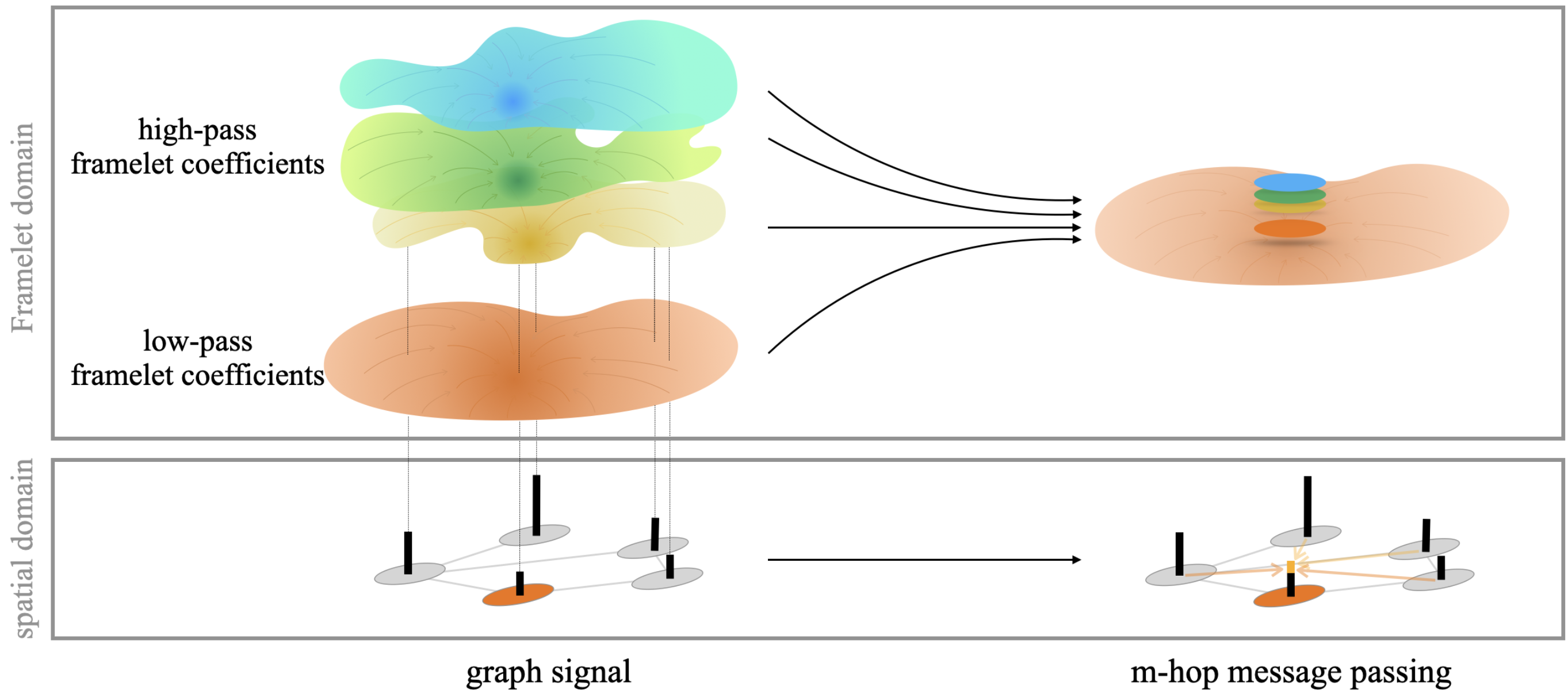
Figure 1: An illustrative workflow of the proposed framelet message passing. An input graph signal is first decomposed into multi-scale coefficients (colored polygons) in the framelet domain. In a convolution layer, each of the framelet coefficients aggregates m-hop neighbors’ coefficients from the same level and scale to update its representation. The multi-scale node representation is then summed up as the propagated new representation of the node. In comparison, multiple spatial-based graph convolution layers are required to accelerate the same range of node information, and they are poor at memorizing long-range information.

To tackle the issue of separately constructing spectral graph convolutions or spatial message passing rules, this work establishes a spectral message passing scheme with multiscale graph framelet transforms. For a given graph, framelet decomposition generates a set of framelet coefficients in the spectral domain with low-pass and high-pass filters. The coefficients with respect to individual nodes then follow the message passing scheme (Gilmer et al., 2017) to integrate their neighborhood information from the same level. The proposed framelet message passing (FMP) has shown promising theoretical properties.

First, it can limit oversmoothing with a non-decay Dirichlet energy during propagation, and the Dirichlet energy would not explode when the network goes deep. Unlike the conventional message passing convolutions that have to repeat $m$ times to cover a relatively large range of $m$-hop neighbors for a central node, the framelet message passing reaches out all $m$-hop neighbors in a single graph convolutional layer. Instead of cutting down the influence of distant neighboring nodes by the gap to the central node, the framelet way disperses small and large ranges of neighboring communities in different scales and levels, where in low-pass framelet coefficients the local approximated information is retained, and high-pass coefficients mainly hold local detailed information. On each of the scales when conducting message passing, the $m$-hop information is adaptively accumulated to the central node, which can be considered as an analog to the graph rewiring, and it is helpful for circumventing the long-standing oversmoothing issue in graph representation learning.

Meanwhile, FMP is stable on perturbed node features. Transforming the graph signal from the spatial domain to the framelet domain divides uncertainties from the corrupted input signal. Through controlling the variance within an acceptable range in separate scales, we prove that the processed representation steadily roams within a range, i.e., the framelet message passing is stable to small input perturbations.

In addition, FMP bypasses unnecessary spectral transforms and improves convolutional efficiency. On top of approaching long-range neighbors in one layer, FMP also avoids the inverse framelet transforms in the traditional framelet convolution (Zheng et al., 2021) and integrates the low and high pass features by adjusting their feature-wise learnable weights in the aggregation.

The rest of the paper starts by introducing the message passing framework in Section 2, and discussing its weakness in the oversmoothing issue in Section 3. Based on the established graph Framelet system and its favorable properties (Section 4). Based on this, Section 5 gives the two variants of the proposed FMP, whose energy-preserving effect and stability are justified in Section 6 and 7, respectively. The empirical performances of FMP are reported in Section 8 for node classification tasks on homogeneous and heterogeneous graphs, where FMP achieves state-of-the-art performance. We review the previous literature in the community in Section 9, and then conclude the work in Section 10.

2 Graph Representation Learning with Message Passing

An undirected attributed graph ${\mathcal{G}}=({\mathcal{V}},{\mathcal{E}},{\bm{X}})$ consists of a non-empty finite set of $n=|{\mathcal{V}}|$ nodes ${\mathcal{V}}$ and a set of edges ${\mathcal{E}}$ between node pairs. Denote ${\bm{A}}\in\mathbb{R}^{N\times N}$ the (weighted) graph adjacency matrix and ${\bm{X}}\in\mathbb{R}^{N\times d}$ the node attributes. A graph convolution learns a matrix representation ${\bm{H}}$ that embeds the structure ${\bm{A}}$ and feature matrix ${\bm{X}}=\{{\bm{X}}_{j}\}_{j=1}^{N}$ with ${\bm{X}}_{j}$ for node $j$.

Message passing (Gilmer et al., 2017) defines a general framework of feature propagation rules on a graph, which updates a central node’s smooth representation by aggregated information (e.g., node attributes) from connected neighbors. At a specific layer $t$, the propagation for the $i$th node reads

$${\bm{X}}_{i}^{(t)} =\gamma\left({\bm{X}}^{(t-1)}_{i},{\bm{Z}}^{(t)}\right)$$ (1)

$${\bm{Z}}^{(t)} =\square_{j\in\mathcal{N}(i)}\phi({\bm{X}}^{(t-1)}_{i},{\bm{X}}^{(t-1)}_{j},{\bm{A}}_{ij}),$$

where $\square(\cdot)$ is a differentiable and permutation invariant aggregation function, such as summation, average, or maximization. Next, the aggregated representation of neighbor nodes ${\bm{Z}}^{(t)}$ is used to update the central node’s representation, where two example operations are addition and concatenation. Both $\gamma(\cdot)$ and $\phi(\cdot)$ are differentiable aggregation functions, such as MLPs. The node set ${\mathcal{N}}(i)$ includes ${\mathcal{V}}_{i}$ and other nodes that are connected directly with ${\mathcal{V}}_{i}$ by an edge, which we call node ${\mathcal{V}}_{i}$’s 1-hop neighbors.

The majority of (spatial-based) graph convolutional layers are designed following the message passing scheme when updating the node representation. For instance, GCN (Kipf and Welling, 2017) adds up the degree-normalized node attributes from neighbors (including itself) and defines

$${\bm{X}}_{i}^{(t)}=\sigma\left(\sum_{j\in\mathcal{N}(i)\cup\{i\}}\frac{1}{\sqrt{1+d_{i}}\sqrt{1+d_{j}}}{\bm{X}}_{j}^{(t-1)}{\bm{W}}\right),$$

where ${\bm{W}}$ is learnable weights, $d_{i}=\sum_{j\in\mathcal{N}(i)}{\bm{A}}_{i,j}$ and ${\bm{D}}={\rm diag}(d_{1},\dots,d_{N})$ is the degree matrix for ${\bm{A}}$. Instead of the pre-defined adjacency matrix, GAT (Veličković et al., 2018) aggregates neighborhood attributes by learnable attention scores and GraphSage (Hamilton et al., 2017) averages the contribution from the sampled neighborhood. Alternatively, GIN (Xu et al., 2019) attaches a custom number of MLP layers for $\square(\cdot)$ after the vanilla summation. While these graph convolutions construct different formulations, they merely make a combination of inner product, transpose, and diagonalization operations on the graph adjacency matrix, which fails to distinguish different adjacency matrice by the 1-WL test (Balcilar et al., 2021). In contrast, spectral-based graph convolutions require eigenvalues or eigenvectors to construct the update rule and create expressive node representations towards the theoretical limit of the 3-WL test.

On top of the expressivity issue, spectral-based convolutions have also proven to ease the stability concern that is widely observed in conventional spatial-based methods. To circumvent the two identified problems, we propose a spectral-based message passing scheme for graph convolution, which is stable and has the ability to alleviate the oversmoothing issues.

3 Depth Limitation of Message Passing by Oversmoothing

The depth limitation prevents the performance of many deep GNN models. The problem was first identified by Li et al. (2018), where many popular spatial graph convolutions apply Laplacian smoothing to graph embedding. Shallow GNNs perform global denoising to exclude local perturbations and achieve state-of-the-art performance in many semi-supervised learning tasks. While a small number of graph convolutions has limited expressivity, deeply stacking the layers leads the connected nodes to converge to indistinguishable embeddings. Such an issue is widely known as oversmoothing.

One way to understand the oversmoothing issue is through the Dirichlet energy, which measures the average distance between connected nodes in the feature space. The graph Laplacian of ${\mathcal{G}}$ is defined by ${\mathcal{L}}={\bm{D}}-{\bm{A}}$. Let $\tilde{{\bm{A}}}:={\bm{A}}+{\bm{I}}_{N},\tilde{{\bm{D}}}:={\bm{D}}+{\bm{I}}_{N}$ be the adjacent and degree matrix of graph ${\mathcal{G}}$ augmented with self-loops and the normalized graph Laplacian is defined by $\widetilde{{\mathcal{L}}}:=\widetilde{{\bm{D}}}^{-1/2}{\mathcal{L}}\widetilde{{\bm{D}}}^{-1/2}$. Formally, the Dirichlet energy of a node feature ${\bm{X}}$ from ${\mathcal{G}}$ with normalized $\widetilde{{\mathcal{L}}}$ is defined by

$$E({\bm{X}}) =\mathrm{tr}({\bm{X}}^{\top}\widetilde{{\mathcal{L}}}{\bm{X}})=\frac{1}{2}\sum{\bm{A}}_{ij}\left(\frac{{\bm{X}}_{i}}{\sqrt{1+d_{i}}}-\frac{{\bm{X}}_{j}}{\sqrt{1+d_{j}}}\right)^{2}.$$

The energy evolution provides a direct indicator for the degree of feature expressivity in the hidden space. For instance, Cai and Wang (2020) observed that GCN (Kipf and Welling, 2017) has the Dirichlet energy decaying rapidly to zero as the network depth increases, which indicates the local high-frequency signals are ignored during propagation. It is thus desired that the Dirichlet energy of the encoded features is bounded for deep GNNs.

We start with GCN as an example to illustrate the cause of oversmoothing. Set ${\bm{P}}:={\bm{I}}_{N}-\widetilde{{\mathcal{L}}}$. It is observed in Oono and Suzuki (2019) that a multi-layer GCN simply writes in the form $f=f_{L}\circ\cdots\circ f_{1}$ where $f_{l}:\mathbb{R}^{N\times d}\rightarrow\mathbb{R}^{N\times d}$ is defined by $f_{l}({\bm{X}}):=\sigma\left({\bm{P}}{\bm{X}}{\bm{W}}_{l}\right)$. Although the asymptotic behavior of the output $X^{(L)}$ of the $\mathrm{GCN}$ as $L\rightarrow\infty$ is investigated in Oono and Suzuki (2019) with oversmoothing property, to facilitate the analysis for our model MPNN, we also sketch the proof for completeness here.

Lemma 1 (Oono and Suzuki (2019))

For any ${\bm{X}}\in\mathbb{R}^{n\times d}$, we have

1. $E({\bm{X}}{\bm{W}}_{l})\leq\mu_{\max}^{2}E({\bm{X}})$, where $\mu_{\max}$ denotes the singular value for ${\bm{W}}_{l}$ with the largest absolute value.

2. $E(\sigma({\bm{X}}))\leq E({\bm{X}})$.

Lemma 2 (Oono and Suzuki (2019))

Without loss of generality, we suppose ${\mathcal{G}}$ is connected. Let $\lambda_{1}\leq\cdots\leq\lambda_{n}$ be the eigenvalue of ${\bm{P}}$ sorted in ascending order. Then, we have

1. $-1<\lambda_{1},\lambda_{n-1}<1$, and $\lambda_{n}=1$, hence $\lambda_{\max}:=\max_{i=1}^{n-1}\left|\lambda_{i}\right|<1$.

2. $E({\bm{P}}{\bm{X}})\leq\lambda_{\max}^{2}E({\bm{X}})$.

Proof  Note that ${\bm{P}}$ and $\widetilde{{\mathcal{L}}}$ share the same eigenspace and the Dirichlet energy is closely associated with the spectrum of ${\bm{P}}$ and $\widetilde{{\mathcal{L}}}$. Recall that ${\bm{P}}={\bm{I}}_{N}-\widetilde{{\mathcal{L}}}=\widetilde{{\bm{D}}}^{-1/2}\widetilde{{\bm{A}}}\widetilde{{\bm{D}}}^{-1/2}$. Since the matrix similarity between ${\bm{P}}$ and $\widetilde{{\bm{D}}}^{-1}\widetilde{{\bm{A}}}$, it suffices to investigate the spectrum of $\widetilde{{\bm{D}}}^{-1}\widetilde{{\bm{A}}}$. Let $\tilde{\lambda}_{1}\leq\cdots\leq\tilde{\lambda}_{n}$ be the eigenvalue of ${\bm{P}}$ sorted in ascending order. It can be verified that $\widetilde{{\bm{D}}}^{-1}\widetilde{{\bm{A}}}$ is a stochastic matrix; hence, by Perron–Frobenius theorem, we have $-1<\tilde{\lambda}_{1},\leq\tilde{\lambda}_{n-1}<1$ and $\tilde{\lambda_{n}}=1$ and $\mathbf{1}$ is the only eigenvector corresponding to $\lambda_{n}=1$. Then, we conclude the first claim. Moreover, we obtain $\widetilde{{\mathcal{L}}}$ is symmetric positive semi-definite matrix with eigenvalues $0=\lambda^{{\mathcal{L}}}_{1}<\lambda^{{\mathcal{L}}}_{2}<\cdots<\lambda^{{\mathcal{L}}}_{n}<2$ and $\mathbf{1}$ is the only eigenvector corresponding to $\lambda^{{\mathcal{L}}}_{1}=0$. Combing the fact that $E({\bm{X}})=\mathrm{tr}({\bm{X}}^{\top}\widetilde{{\mathcal{L}}}{\bm{X}})$ we conclude $E({\bm{P}}{\bm{X}})\leq\lambda_{\max}^{2}E({\bm{X}})$. It means the graph convolution contracts the energy by a factor of $\lambda_{\max}^{2}$, and we also get a by-product that the convolution shrinks the feature ${\bm{X}}$ except for the constant component.  

By the above Lemmas, we obtain the oversmoothing property of GCN as

Theorem 3 (Oono and Suzuki (2019))

Let ${\rm GCN}_{L}:=f_{L}\circ f_{L-1}\circ\cdots\circ f_{1}$ be a graph convolutional network with $L$ layers with input feature $X$. Then, the Dirichlet energy of ${\rm GCN}_{L}$ is bounded by

$$E({\rm GCN}_{L}({\bm{X}}))<\left(\mu_{\max}\lambda_{\max}\right)^{2L}E({\bm{X}}).$$ (2)

Suppose the $\mu_{\max}\lambda_{\max}<1$, then the energy decays exponentially with layers.

4 Undecimated Framelet System

The $\{{\bm{g}}_{\ell}\}_{\ell=1}^{M}$ from $l_{2}({\mathcal{G}})$ is said a frame for $l_{2}({\mathcal{G}})$ is a collection of elements if there exist constants $A$ and $B$, $0<A\leq B<\infty$, such that

$$A\|{\bm{f}}\|^{2}\leq\sum_{\ell=1}^{M}|\left\langle{\bm{f}},{\bm{g}}_{\ell}\right\rangle|^{2}\leq B\|{\bm{f}}\|^{2}\quad\forall{\bm{f}}\in l_{2}({\mathcal{G}}).$$ (3)

Here $A,B$ are called frame bounds. When $A=B=1$, $\{{\bm{g}}_{\ell}\}_{\ell=1}^{M}$ is said to form a tight frame for $l_{2}({\mathcal{G}})$. In this case, (3) is alternatively written as

$${\bm{f}}=\sum_{\ell=1}^{M}\left\langle{\bm{f}},{\bm{g}}_{\ell}\right\rangle{\bm{g}}_{\ell},$$ (4)

which follows from the polarization identity. For a tight frame $\{{\bm{g}}_{\ell}\}_{\ell=1}^{M}$ with $\|{\bm{g}}_{\ell}\|=1$ for $\ell=1,\dots,M$, there must holds $M=N$, and $\{{\bm{g}}_{\ell}\}_{\ell=1}^{N}$ forms an orthonormal basis for $l_{2}({\mathcal{G}})$. Tight frames ensures the one-to-one mapping between framelet coefficients $\left\langle{\bm{f}},{\bm{g}}_{\ell}\right\rangle$ and the original vector ${\bm{f}}$ (Daubechies, 1992).

Let $\Psi=\{\alpha;\beta^{(1)},\dots,\beta^{(K)}\}$ be a set of functions in $L_{1}(\mathbb{R})$, where $L_{1}(\mathbb{R})$ refers to the functions that are absolutely integrable on $\mathbb{R}$ with respect to the Lebesgure measure. The Fourier transform $\widehat{\gamma}$ of a function $\gamma\in L_{1}(\mathbb{R})$ is defined by $\widehat{\gamma}(\xi):=\int_{\mathbb{R}}\gamma(t)e^{-2\pi it\xi}\>\mathrm{d}t$, where $\xi\in\mathbb{R}$. The Fourier transform can be extended from $L_{1}(\mathbb{R})$ to $L_{2}(\mathbb{R})$, which is the space of square-integrable functions on $\mathbb{R}$. See Stein and Shakarchi (2011) for further information.

A filter bank is a set of filters, where a filter (or mask) $h:=\{h_{k}\}_{k\in{\mathbb{Z}}}\subseteq{\mathbb{C}}$ is a complex-valued sequence in $l_{1}({\mathbb{Z}}):=\{h=\{h_{k}\}_{k\in{\mathbb{Z}}}\subseteq{\mathbb{C}}:\sum_{k\in{\mathbb{Z}}}|h_{k}|<\infty\}$. The Fourier series of a sequence $\{h_{k}\}_{k\in{\mathbb{Z}}}$ is the $1$-periodic function $\widehat{h}(\xi):=\sum_{k\in{\mathbb{Z}}}h_{k}e^{-2\pi ik\xi}$ with $\xi\in\mathbb{R}$. Let $\Psi=\{\alpha;\beta^{(1)},\dots,\beta^{(K)}\}$ be a set of framelet generators associated with a filter bank $\bm{\eta}:=\{a;b^{(1)},\ldots,b^{(K)}\}$. Then the Fourier transforms of the functions in $\Psi$ and the filters’ corresponding Fourier series in $\bm{\eta}$ satisfy

$$\widehat{\alpha}(2\xi)=\widehat{a}(\xi)\widehat{\alpha}(\xi),\quad\widehat{\beta^{(r)}}(2\xi)=\widehat{b^{(r)}}(\xi)\widehat{\alpha}(\xi),\quad r=1,\ldots,K,\;\xi\in\mathbb{R}.$$ (5)

We give two typical examples of filters and scaling functions, as follows.

Example.1

The first one is the Haar-type filters with one high pass: for $\xi\in\mathbb{R}$,

$$\widehat{a}(\xi)=\cos(\xi/2),\quad\widehat{b^{(1)}}(\xi)=\sin(\xi/2)$$ (6)

with scaling functions

$$\widehat{\alpha}(\xi)=\frac{\sin(\xi/2)}{\xi/2},\quad\widehat{\beta}(\xi)=\sqrt{1-\left(\frac{\sin(\xi/2)}{\xi/2}\right)^{2}}.$$

Example.2

Another example of filters and scaling functions with two high passes are from (Daubechies, 1992, Chapter 4):

$$\widehat{a}(\xi) :=\left\{\begin{array}[]{ll}1,&|\xi|<\frac{1}{8},\\[2.84526pt] \cos\bigl{(}\frac{\pi}{2}\hskip 0.85358pt\nu(8|\xi|-1)\bigr{)},&\frac{1}{8}\leq|\xi|\leq\frac{1}{4},\\[2.84526pt] 0,&\frac{1}{4}<|\xi|\leq\frac{1}{2},\end{array}\right.$$ (7d)

$$\widehat{b^{(1)}}(\xi) :=\left\{\begin{array}[]{ll}0,&|\xi|<\frac{1}{8},\\[2.84526pt] \sin\bigl{(}\frac{\pi}{2}\hskip 0.85358pt\nu(8|\xi|-1)\bigr{)},&\frac{1}{8}\leq|\xi|\leq\frac{1}{4},\\[2.84526pt] \cos\bigl{(}\frac{\pi}{2}\hskip 0.85358pt\nu(4|\xi|-1)\bigr{)},&\frac{1}{4}<|\xi|\leq\frac{1}{2}.\end{array}\right.$$ (7h)

$$\widehat{b^{(2)}}(\xi) :=\left\{\begin{array}[]{ll}0,&|\xi|<\frac{1}{4},\\[2.84526pt] \sin\bigl{(}\frac{\pi}{2}\hskip 0.85358pt\nu(4|\xi|-1)\bigr{)},&\frac{1}{4}\leq|\xi|\leq\frac{1}{2},\end{array}\right.$$ (7k)

where

$$\nu(t):=t^{4}(35-84t+70t^{2}-20t^{3}),\quad t\in\mathbb{R}.$$

The associated framelet generators $\Psi=\{\alpha;\beta^{1},\beta^{2}\}$ are defined by

$$\widehat{\alpha}(\xi) =\left\{\begin{array}[]{ll}1,&|\xi|<\frac{1}{4},\\[2.84526pt] \cos\bigl{(}\frac{\pi}{2}\hskip 0.85358pt\nu(4|\xi|-1)\bigr{)},&\frac{1}{4}\leq|\xi|\leq\frac{1}{2},\\[2.84526pt] 0,&\hbox{else},\end{array}\right.$$ (8d)

$$\widehat{\beta^{1}}(\xi) =\left\{\begin{array}[]{ll}\sin\left(\frac{\pi}{2}\hskip 0.85358pt\nu(4|\xi|-1)\right),&\frac{1}{4}\leq|\xi|<\frac{1}{2},\\[2.84526pt] \cos^{2}\left(\frac{\pi}{2}\hskip 0.85358pt\nu(2|\xi|-1)\right),&\frac{1}{2}\leq|\xi|\leq 1,\\[2.84526pt] 0,&\hbox{else},\end{array}\right.$$ (8h)

$$\widehat{\beta^{2}}(\xi) =\left\{\begin{array}[]{ll}0,&|\xi|<\frac{1}{2},\\[2.84526pt] \cos\left(\frac{\pi}{2}\hskip 0.85358pt\nu(2|\xi|-1)\right)\sin\left(\frac{\pi}{2}\hskip 0.85358pt\nu(2|\xi|-1)\right),&\frac{1}{2}\leq|\xi|\leq 1,\\[2.84526pt] 0,&\hbox{else}.\end{array}\right.$$ (8l)

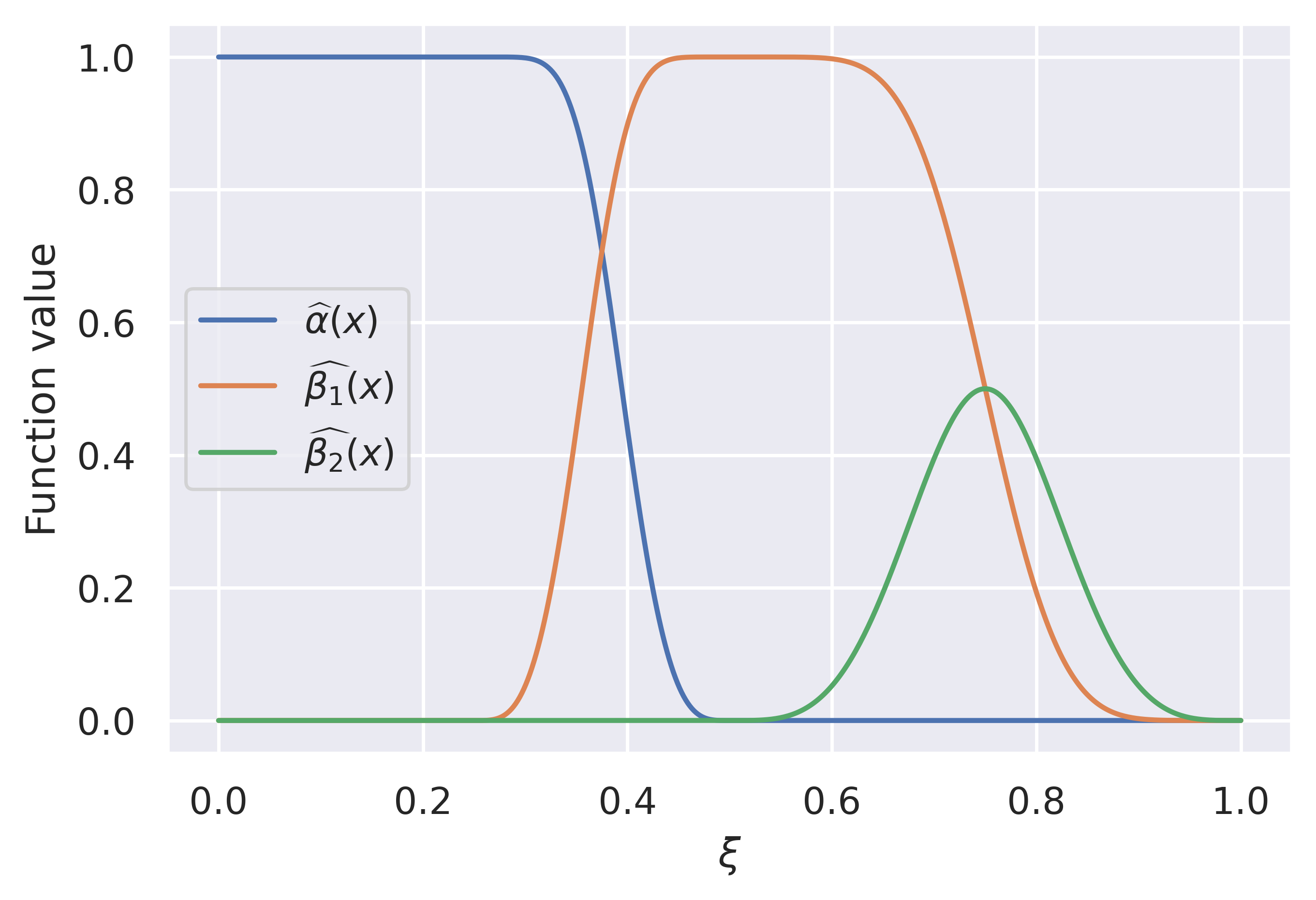
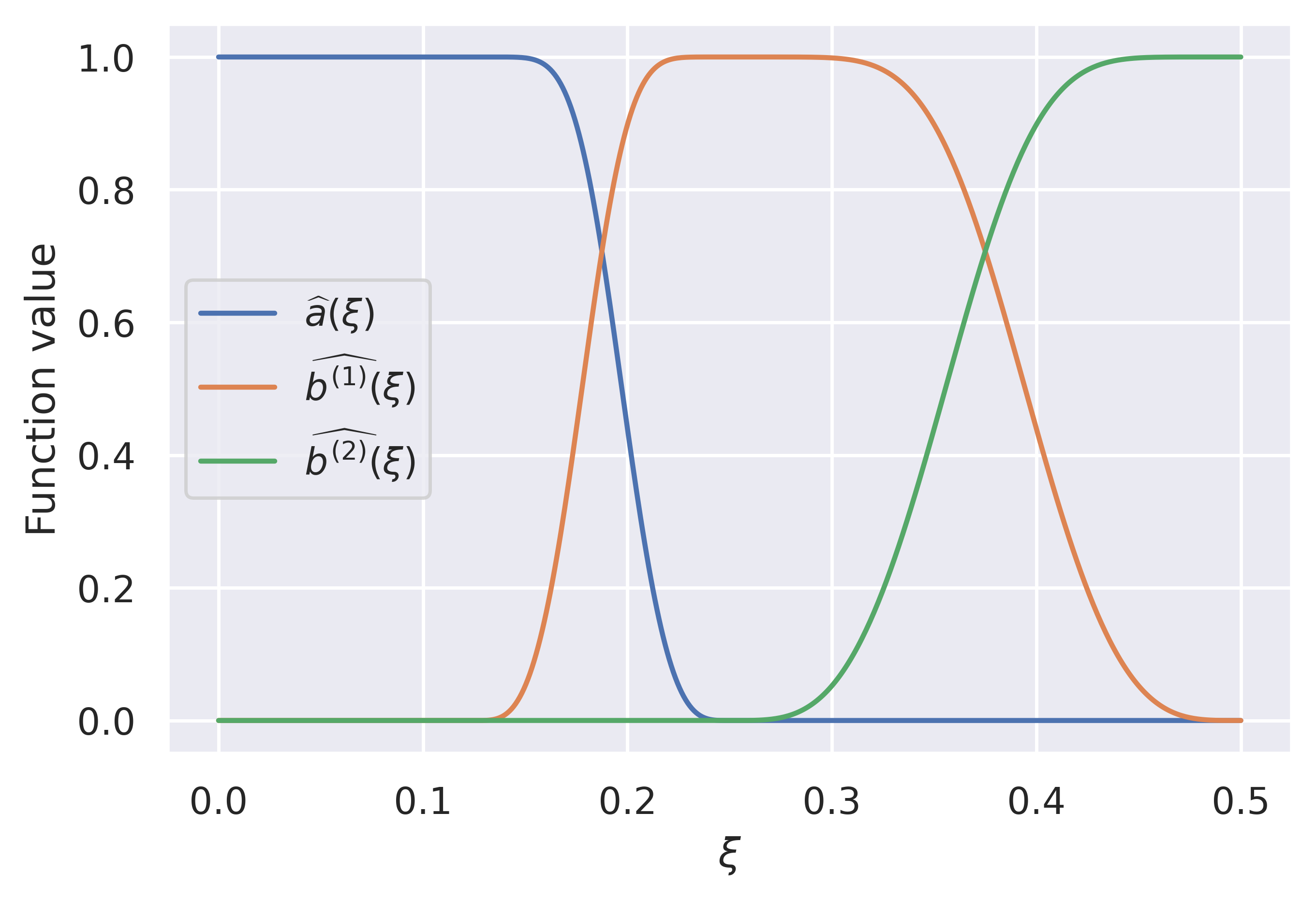
Figure 2: Filters and Scaling functions with two high passes in (7) and (8).

Definition 4 (Undecimated Framelet System (Dong, 2017; Zheng et al., 2022))

Given a filter bank $\bm{\eta}:=\{a;b^{(1)},\dots,b^{(K)}\}$ and scaling functions $\Psi=\{\alpha;\beta^{(1)},\dots,\beta^{(K)}\}$, an undecimated framelet system $\operatorname{UFS}_{J_{1}}^{J}(\Psi,\bm{\eta})$ ($J>J_{1}$) for $l_{2}({\mathcal{G}})$ from $J_{1}$ to $J$ is defined by

$$\operatorname{UFS}_{J_{1}}^{J}(\Psi,\bm{\eta}) :=\operatorname{UFS}_{J_{1}}^{J}(\Psi,\bm{\eta};{\mathcal{G}})$$

$$:=\left\{\varphi_{J_{1},p}:p\in{\mathcal{V}}\right\}\cup\{\psi_{l,p}^{(k)}:p\in{\mathcal{V}},l=J_{1},\dots,J\}_{k=1}^{K}.$$

In this paper, we focus on undecimated framelets, which maintain a constant number of framelets at each level of the decomposition. Decimated framelet systems, on the other hand, can be created by constructing a coarse-grained chain for the graph, as described in detail in Zheng et al. (2022).

To ensure computational efficiency, Haar-type filters are adopted when generating the scaling functions, which defines $\widehat{a}(x)=\cos(x/2)$ and $\widehat{b^{(1)}}(x)=\sin(x/2)$ for $x\in\mathbb{R}$. Alternatively, other types of filters, such as linear or quadratic filters, could also be considered as described in Dong (2017).

Suppose $l\in{\mathbb{Z}}$ and $p\in{\mathcal{V}}$, the undecimated framelets $\bm{\varphi}_{l,p}(v)$ and $\bm{\psi}_{l,p}^{r}(v)$, $v\in{\mathcal{V}}$ at scale $l$ are filtered Bessel kernels (or summability kernels), which are constructed following

$$\bm{\varphi}_{l,p}(v) :=\sum_{\ell=1}^{N}\widehat{\alpha}\left(\frac{\lambda_{\ell}}{2^{l}}\right)\overline{{\bm{u}}_{\ell}(p)}{\bm{u}}_{\ell}(v),$$ (9)

$$\bm{\psi}_{l,p}^{r}(v) :=\sum_{\ell=1}^{N}\widehat{\beta^{(r)}}\left(\frac{\lambda_{\ell}}{2^{l}}\right)\overline{{\bm{u}}_{\ell}(p)}{\bm{u}}_{\ell}(v),\quad r=1,\ldots,K.$$

We say $\bm{\varphi}_{l,p}(v)$ and $\bm{\psi}_{l,p}^{r}(v)$ are with respect to the “dilation” at scale $l$ and the “translation” for the vertex $p\in{\mathcal{V}}$. The construction of framelets are analogs of those of wavelets in $\mathbb{R}^{d}$. The functions $\alpha,\beta^{(r)}$ of $\Psi$ are named framelet generators or scaling functions for the undecimated framelet system.

Theorem 5 (Equivalence Conditions of Framelet Tightness, (Zheng et al., 2022))

Let ${\mathcal{G}}=({\mathcal{V}},{\mathcal{E}},{\bm{W}})$ be a graph and $\{({\bm{u}}_{\ell},\lambda_{\ell})\}_{\ell=1}^{N}$ be a set of orthonormal eigenpairs for $l_{2}({\mathcal{G}})$. Let $\Psi=\{\alpha;\beta^{(1)},\dots,\beta^{(K)}\}$ be a set of functions in $L_{1}(\mathbb{R})$ with respect to a filter bank $\bm{\eta}=\{a;b^{(1)},\ldots,b^{(K)}\}$ that satisfies (5). An undecimated framelet system is denoted by $\mathsf{UFS}_{J_{1}}^{J}(\Psi,\bm{\eta};{\mathcal{G}}),J_{1}=1,\ldots,J$ ($J\geq 1$) with framelets $\bm{\varphi}_{l,p}$ and $\bm{\psi}_{l,p}^{r}$ in (9). Then, the following statements are equivalent.

• For each $J_{1}=1,\ldots,J$, the undecimated framelet system $\mathsf{UFS}_{J_{1}}^{J}(\Psi,\bm{\eta};{\mathcal{G}})$ is a tight frame for $l_{2}({\mathcal{G}})$, that is, $\forall f\in l_{2}({\mathcal{G}})$,

  $$\|f\|^{2}=\sum_{p\in V}\Big{|}\left\langle f,\bm{\varphi}_{J_{1},p}\right\rangle\Big{|}^{2}+\sum_{l=J_{1}}^{J}\sum_{r=1}^{K}\sum_{p\in V}\Big{|}\left\langle f,\bm{\psi}_{l,p}^{r}\right\rangle\Big{|}^{2}.$$ (10)

• For all $f\in l_{2}({\mathcal{G}})$ and for $l=1,\ldots,J-1$, the following identities hold:

  $$f=\sum_{p\in V}\left\langle f,\bm{\varphi}_{J,p}\right\rangle\bm{\varphi}_{J,p}+\sum_{r=1}^{K}\sum_{p\in V}\left\langle f,\bm{\psi}_{J,p}^{r}\right\rangle\bm{\psi}_{J,p}^{r},$$ (11)

  $$\sum_{p\in V}\left\langle f,\bm{\varphi}_{l+1,p}\right\rangle\bm{\varphi}_{l+1,p}=\sum_{p\in V}\left\langle f,\bm{\varphi}_{l,p}\right\rangle\bm{\varphi}_{l,p}+\sum_{r=1}^{K}\sum_{p\in V}\left\langle f,\bm{\psi}_{l,p}^{r}\right\rangle\bm{\psi}_{l,p}^{r}.$$ (12)

• For all $f\in l_{2}({\mathcal{G}})$ and for $l=1,\ldots,J-1$, the following identities hold:

  $$\|f\|^{2}=\sum_{p\in V}\bigl{|}\left\langle f,\bm{\varphi}_{J,p}\right\rangle\bigr{|}^{2}+\sum_{r=1}^{K}\sum_{p\in V}\bigl{|}\left\langle f,\bm{\psi}_{J,p}^{r}\right\rangle\bigr{|}^{2},\quad$$ (13)

  $$\sum_{p\in V}\bigl{|}\left\langle f,\bm{\varphi}_{l+1,p}\right\rangle\bigr{|}^{2}=\sum_{p\in V}\bigl{|}\left\langle f,\bm{\varphi}_{l,p}\right\rangle\bigr{|}^{2}+\sum_{r=1}^{K}\sum_{p\in V}\bigl{|}\left\langle f,\bm{\psi}_{l,p}^{r}\right\rangle\bigr{|}^{2}.$$ (14)

• The functions in $\Psi$ satisfy

  $$1=\left|\widehat{\alpha}\left(\frac{\lambda_{\ell}}{2^{J}}\right)\right|^{2}+\sum_{r=1}^{K}\left|\widehat{\beta^{(r)}}\left(\frac{\lambda_{\ell}}{2^{J}}\right)\right|^{2} \quad\forall\ell=1,\ldots,N,$$ (15)

  $$\left|\widehat{\alpha}\left(\frac{\lambda_{\ell}}{2^{l+1}}\right)\right|^{2}=\left|\widehat{\alpha}\left(\frac{\lambda_{\ell}}{2^{l}}\right)\right|^{2}+\sum_{r=1}^{K}\left|\widehat{\beta^{(r)}}\left(\frac{\lambda_{\ell}}{2^{l}}\right)\right|^{2} \quad\forall\begin{array}[]{l}\ell=1,\ldots,N,\\ l=1,\ldots,J-1.\end{array}$$ (18)

• The identities in (15) hold and the filters in the filter bank $\bm{\eta}$ satisfy

  $$\left|\widehat{a}\left(\frac{\lambda_{\ell}}{2^{l}}\right)\right|^{2}+\sum_{r=1}^{K}\left|\widehat{b^{(r)}}\left(\frac{\lambda_{\ell}}{2^{l}}\right)\right|^{2}=1\quad\forall\ell\in\sigma_{\alpha}^{(l)},\;l=2,\ldots,J,$$ (19)

  with

  $$\sigma_{\alpha}^{(l)}:=\left\{\ell\in\{1,\ldots,N\}:\widehat{\alpha}\left(\frac{\lambda_{\ell}}{2^{l}}\right)\neq 0\right\}.$$

Remark 6

In this paper, we use $2$-norm.

5 Graph Framelet Message Passing

The aggregation of framelet coefficients for the neighborhood of the node $i$ takes over up to the $m$-th multi-hop $\mathcal{N}^{m}(i)$.

5.1 Graph Framelet Transforms

In a spectral-based graph convolution, graph signals are transformed to a set of coefficients $\hat{{\bm{X}}}=\bm{{\mathcal{W}}}{\bm{X}}^{\rm in}$ in frequency channels by the decomposition operator $\bm{{\mathcal{W}}}$. The learnable filters are then trained for the spectral coefficients to approach node-level representative graph embeddings.

This work implements undecimated framelet transforms (Zheng et al., 2021) that generate a set of multi-scale and multi-level framelet coefficients for the input graph signal, where the low-pass coefficients include general global trend of ${\bm{X}}$, and the high-pass coefficients portray the local properties of the graph attributes at different degrees of detail. Consequently, conducting framelet transforms on a graph avoids trivially smoothing out rare patterns to preserve more energy for the graph representation and alleviate the oversmoothing issue during message aggregation.

Recall that the orthonormal bases at different levels ($l$) and scales ($r$) formulate the framelet decomposition operators $\bm{{\mathcal{W}}}_{r,l}$, , which is applied to obtain the framelet coefficients $\hat{{\bm{X}}}$. In particular, $\bm{{\mathcal{W}}}_{0,J}$ is composed of the low-pass framelet basis $\bm{\varphi}_{J,p},\;p\in{\mathcal{V}}$ for the low-pass coefficient matrix, i.e., $\hat{{\bm{X}}}=\bm{{\mathcal{W}}}_{0,J}{\bm{X}}$ that approximates the global graph information. Meanwhile, the high-pass coefficient matrices $\bm{{\mathcal{W}}}_{r,l}{\bm{X}}$ with $r=1,\dots,K,\;l=1,\dots,J$ that record detailed local graph characteristics in different scale levels are decomposed by the associated high-pass framelet bases $\bm{\psi}_{l,p}^{(r)}$. Generally, framelet coefficients at larger scales contain more localized information with smaller energy.

As the framelet bases $\bm{\varphi}_{l,p},\bm{\psi}_{l,p}^{(r)}$ are defined by eigenpairs of the normalized graph Laplacian $\widetilde{{\mathcal{L}}}$, the associated framelet coefficients can be recursively formulated by filter matrices. Specifically, denote the eigenvectors ${\bm{U}}=[{\bm{u}}_{1},\dots,{\bm{u}}_{N}]\in\mathbb{R}^{N\times N}$ and the eigenvalues $\Lambda=\operatorname{diag}(\lambda_{1},\dots,\lambda_{N})$ for the normalized graph Laplacian $\widetilde{{\mathcal{L}}}$, for the low pass and the $r$th high pass,

$$\bm{{\mathcal{W}}}_{0,J}{\bm{X}}={\bm{U}}\widehat{\alpha}\left(\frac{\Lambda}{2}\right){\bm{U}}^{\top}{\bm{X}},$$ (20)

$$\bm{{\mathcal{W}}}_{r,l}{\bm{X}}={\bm{U}}\widehat{\beta^{(r)}}\left(\frac{\Lambda}{2^{l+1}}\right){\bm{U}}^{\top}{\bm{X}}\quad\forall l=1,\dots,J.$$

Alternatively, Chebyshev polynomials approximation is a valid solution to achieve efficient and scalable framelet decomposition (Dong, 2017; Zheng et al., 2021) by avoiding time-consuming eigendecomposition. Let $m$ be the highest order of the Chebyshev polynomial involved. Denote the $m$-order approximation of $\alpha$ and $\{\beta^{(r)}\}_{r=1}^{K}$ by ${\mathcal{T}}_{0}$ and $\{{\mathcal{T}}_{r}\}_{r=1}^{K}$, respectively. The approximated framelet decomposition operator $\bm{{\mathcal{W}}}^{\natural}_{r,l}$ (including $\bm{{\mathcal{W}}}^{\natural}_{0,J}$) is defined as products of Chebyshev polynomials of the graph Laplacian ${\mathcal{L}}$, i.e.,

$$\bm{{\mathcal{W}}}^{\natural}_{r,l}=\begin{cases}{\mathcal{T}}_{0}\left(2^{-R}{\mathcal{L}}\right),&l=1,\\[2.84526pt] {\mathcal{T}}_{k}\left(2^{R+l-1}{\mathcal{L}}\right){\mathcal{T}}_{0}\left(2^{R+l-2}{\mathcal{L}}\right)\dots\mathcal{T}_{0}\left(2^{-R}{\mathcal{L}}\right),&l=2,\dots,J.\end{cases}$$

Here the real-value dilation scale $R$ is the smallest integer such that $\lambda_{\max}=\lambda_{N}\leq 2^{R}\pi$. In this definition, it is required for the finest scale $1/2^{K+J}$ that guarantees $\lambda_{\ell}/2^{K+J-l}\in(0,\pi)$ for $\ell=1,2,...,N$.

Chebyshev polynomials approximation not only achieves efficient calculation to obtain framelet coefficients for the nodes, but also collects information from the nodes’ neighbors in the framelet domain of the same channel. In particular, the aggregation of framelet coefficients for the neighborhood of the node $i$ takes over up to the $m$-hop $\mathcal{N}^{m}(i)$. Based on this, we propose the general framelet message passing framework.

5.2 Framelet Message Passing

We follow the general message passing scheme in Equation (1) and define the vanilla Framelet message passing (FMP) for the graph node feature ${\bm{X}}^{(t)}$ at layer $t$ by

$${\bm{X}}_{i}^{(t)} ={\bm{X}}_{i}^{(t-1)}+{\bm{Z}}_{i}^{(t)}$$ (21)

$${\bm{Z}}_{i}^{(t)} =\sigma\left(\sum_{j\in\mathcal{N}^{m}(i)}\left(\sum_{r=1}^{K}\sum_{l=1}^{J}(\bm{{\mathcal{W}}}^{\natural}_{r,l})_{i,j}{\bm{X}}_{j}^{(t-1)}\Theta_{r}+(\bm{{\mathcal{W}}}^{\natural}_{0,J})_{i,j}{\bm{X}}_{j}^{(t-1)}\Theta_{0}\right)\right),$$

where the propagated feature ${\bm{Z}}_{i}^{(t)}$ at node $i$ sums over the low and high passes coefficients at all scales, $\sigma$ is the ReLU activation function, and $\Theta_{r}\in\mathbb{R}^{d\times d}$ are learnable parameter square matrices associated with the high passes and low pass, with the size $d$ equal to the number of features of $X^{(t-1)}$.

The framelet message passing has the matrix form

$${\bm{X}}^{(t)} ={\bm{X}}^{(t-1)}+{\bm{Z}}^{(t)}$$ (22)

$${\bm{Z}}^{(t)} =\sigma\left(\sum_{r=1}^{K}\sum_{l=1}^{J}(\bm{{\mathcal{W}}}^{\natural}_{r,l}){\bm{X}}^{(t-1)}\Theta_{r}+(\bm{{\mathcal{W}}}^{\natural}_{0,J}){\bm{X}}^{(t-1)}\Theta_{0}\right).$$

As shown in the previous formulation, the aggregation takes over up to $m$-hop neighbours of the target node $i$. It exploits the framelet coefficients from an $m$-order approximated $\bm{{\mathcal{W}}}^{\natural}_{r,l}$, which involves higher-order graph Laplacians, i.e., ${\mathcal{L}}^{m}$, to make the spectral aggregation as powerful as conducting an $m$-hop neighborhood spatial MPNN (Gilmer et al., 2017). Intuitively, the proposed update rule is thus more efficient than the conventional MPNN schemes in the sense that a single FMP layer is sufficient to reach distant nodes from $m$-hops away. Meanwhile, FMP splits framelet coefficients into different scales and levels instead of implementing a rough global summation, which further preserves the essential local and global patterns and circumvents the oversmoothing issue when stacking multiple convolutional layers.

5.3 Continuous Framelet Message Passing with Neural ODE

The vanilla FMP in Equation (21) formulates a discrete version of spectral feature aggregation of node features. In order to gain extra expressivity for the node embedding, we design a continuous update scheme and formulate an enhanced FMP by neural ODE, such that

$${\partial{\bm{X}}_{i}(t)}/{\partial t}={\bm{Z}}_{i}(t)$$ (23)

$${\bm{Z}}_{i}(t)=\sum_{j\in\mathcal{N}^{m}(i)}\left(\sum_{r=1}^{K}\sum_{l=1}^{J}(\bm{{\mathcal{W}}}^{\natural}_{r,l})_{i,j}{\bm{X}}_{j}{(t)}\Theta_{r}+(\bm{{\mathcal{W}}}^{\natural}_{0,J})_{i,j}{\bm{X}}_{j}{(t)}\Theta_{0}\right)$$

$${\bm{X}}_{i}{(0)}=\text{MLP}({\bm{X}}_{i}).$$

Here ${\bm{X}}_{i}{(t)}$ denotes the encoded features of node $i$ at some timestamp $t$ during a continuous process. The initial state is obtained by a simple MLP layer on the input node feature, i.e., ${\bm{X}}_{i}{(0)}=\text{MLP}({\bm{X}}_{i})$. The last embedding ${\bm{X}}_{i}{(T)}$ can be obtained by numerically solving Equation (LABEL:eq:fmp2) with an ODE solver, which requires a stable and efficient numerical integrator. Since the proposed method is stable during the evolution within finite time, the vast explicit and implicit numerical methods are applicable with a considerable small step size $\Delta t$. In particular, we implement Dormand–Prince5 (DOPRI5) (Dormand and Prince, 1980) with adaptive step size for computational complexity. Note that the practical network depth (i.e., the number of propagation layers) is equal to the numerical iteration number that is specified in the ODE solver.

6 Limited Oversmoothing in Framelet Message Passing

Following the discussion of oversmoothing in Section 3, this section demonstrates that FMP provides a remedy for the oversmoothing predicament by decomposing ${\bm{X}}$ into low-pass and high-pass coefficients with the energy conservation property.

Proposition 7 (Energy conservation)

$$E({\bm{X}})=E(\bm{{\mathcal{W}}}_{0,J}{\bm{X}})+\sum_{r=1}^{K}\sum_{l=1}^{J}E(\bm{{\mathcal{W}}}_{r,l}{\bm{X}}),$$ (24)

where $E(\bm{{\mathcal{W}}}_{0,J}{\bm{X}})$ and $E(\bm{{\mathcal{W}}}_{r,l}{\bm{X}})$ break down the total energy $E({\bm{X}})$ into multi scales, and into low and high passes.

Proof  Recall the facts that $E({\bm{X}})=\mathrm{tr}({\bm{X}}^{\top}\widetilde{{\mathcal{L}}}{\bm{X}})$ and $\widetilde{{\mathcal{L}}}={\bm{U}}\Lambda{\bm{U}}^{\top}$, we have

$$E(\bm{{\mathcal{W}}}_{0,J}{\bm{X}})=\mathrm{tr}\left({\bm{X}}^{\top}\bm{{\mathcal{W}}}_{0,J}^{\top}\widetilde{{\mathcal{L}}}\bm{{\mathcal{W}}}_{0,J}{\bm{X}}\right)=\mathrm{tr}\left({\bm{X}}^{\top}{\bm{U}}\widehat{\alpha}\left(\frac{\Lambda}{2}\right)^{2}\Lambda{\bm{U}}^{\top}{\bm{X}}\right),$$

and $\forall l=1,\dots,J,$

$$E(\bm{{\mathcal{W}}}_{r,l}{\bm{X}})=\mathrm{tr}\left({\bm{X}}^{\top}\bm{{\mathcal{W}}}_{0,J}^{\top}\widetilde{{\mathcal{L}}}\bm{{\mathcal{W}}}_{r,l}{\bm{X}}\right)=\mathrm{tr}\left({\bm{X}}^{\top}{\bm{U}}\widehat{\beta^{(r)}}\left(\frac{\Lambda}{2^{l+1}}\right)^{2}\Lambda{\bm{U}}^{\top}{\bm{X}}\right).$$ (25)

By the identity (18), we also have

$$\widehat{\alpha}\left(\frac{\Lambda}{2}\right)^{2}+\sum_{r=1}^{K}\sum_{l=1}^{J}\widehat{\beta^{(r)}}\left(\frac{\Lambda}{2^{l+1}}\right)^{2}={\bm{I}}.$$ (26)

Therefore, combining (25) and (26), we obtain that

$$E(\bm{{\mathcal{W}}}_{0,J}{\bm{X}})+\sum_{r=1}^{K}\sum_{l=1}^{J}E(\bm{{\mathcal{W}}}_{r,l}{\bm{X}})$$

$$= \mathrm{tr}\left({\bm{X}}^{\top}{\bm{U}}\widehat{\alpha}\left(\frac{\Lambda}{2}\right)^{2}\Lambda{\bm{U}}^{\top}{\bm{X}}\right)+\sum_{r=1}^{K}\sum_{l=1}^{J}\mathrm{tr}\left({\bm{X}}^{\top}{\bm{U}}\widehat{\beta^{(r)}}\left(\frac{\Lambda}{2^{l+1}}\right)^{2}\Lambda{\bm{U}}^{\top}{\bm{X}}\right)$$

$$= \mathrm{tr}\left({\bm{X}}^{\top}{\bm{U}}\left(\widehat{\alpha}\left(\frac{\Lambda}{2}\right)^{2}+\sum_{r=1}^{K}\sum_{l=1}^{J}\widehat{\beta^{(r)}}\left(\frac{\Lambda}{2^{l+1}}\right)^{2}\right)\Lambda{\bm{U}}^{\top}{\bm{X}}\right)$$

$$= \mathrm{tr}\left({\bm{X}}^{\top}{\bm{U}}\Lambda{\bm{U}}^{\top}{\bm{X}}\right)$$

$$= E({\bm{X}}),$$

thus completing the proof.  

For the approximated framelet transforms $\bm{{\mathcal{W}}}^{\natural}_{r,l}$, there is an energy change on RHS of (24) due to the truncation error. The relatively smoother node features account for a lower level energy $E(\bm{{\mathcal{W}}}_{0,J}{\bm{X}})$. In this way, we provide more flexibility to maneuver energy evolution as the energy does not decay when we use FMP in (21) or (LABEL:eq:fmp2). For simplicity, we focus on the exact framelet transforms. Under some mild assumptions on $\Theta_{r}$, we have the following two estimations on the Dirichlet energy.

Lemma 8

(Zhou, 2014) Let ${\bm{A}}_{i}\in\mathbb{R}^{d\times d}$ be positive semi-definite $(i=1,2,\cdots,n)$. Then,

$$\mathrm{tr}\left({\bm{A}}_{1}{\bm{A}}_{2}\cdots{\bm{A}}_{n}\right)\leq\sum_{i=1}^{d}\mu_{i}\left({\bm{A}}_{1}{\bm{A}}_{2}\cdots{\bm{A}}_{n}\right)\leq\mathrm{tr}\left({\bm{A}}_{1}\right)\mathrm{tr}\left({\bm{A}}_{2}\right)\cdots\mathrm{tr}\left({\bm{A}}_{n}\right),$$

where $\mu({\bm{A}})$ denotes the singular value of matrix ${\bm{A}}$.

The following theorem shows for the framelet message passing without activation function in the update, the Dirichlet energy of the feature at the $t$th layer ${\bm{X}}^{(t)}$ is not less than that of the $(t-1)$th layer ${\bm{X}}^{(t-1)}$. In fact, the ${\bm{X}}^{(t)}$ and ${\bm{X}}^{(t-1)}$ are equivalent up to some constant, and the constant with respect to the upper bound depends jointly on the level of the framelet decomposition and the learnable parameters’ bound.

Theorem 9

Let the FMP defined by

$${\bm{X}}^{(t)} ={\bm{X}}^{(t-1)}+{\bm{Z}}^{(t)}$$ (27)

$${\bm{Z}}^{(t)} =\sum_{r=1}^{K}\sum_{l=1}^{J}(\bm{{\mathcal{W}}}_{r,l}){\bm{X}}^{(t-1)}\Theta_{r}+(\bm{{\mathcal{W}}}_{0,J}){\bm{X}}^{(t-1)}\Theta_{0},$$

where the parameter matrix $\Theta_{r}\in\mathbb{R}^{d\times d}\>(r=0,1,\cdots,K)$. Suppose $\Theta_{r}$ is positive semi-definite with $\mathrm{tr}\left(\Theta_{r}\right)\leq M$ for every $r$, then we can bound the Dirichlet energy of the graph node feature ${\bm{X}}^{(t)}$ at layer $t$ by

$$E\left({\bm{X}}^{(t-1))}\right)\leq E\left({\bm{X}}^{(t))}\right)\leq\left(M\sqrt{KJ+1}+1\right)^{2}E\left({\bm{X}}^{(t-1)}\right).$$ (28)

Proof  By definition, we have

$$E\left({\bm{X}}^{(t)}\right) =\mathrm{tr}\left(\left({\bm{X}}^{(t)}\right)^{\top}\widetilde{{\mathcal{L}}}{\bm{X}}^{(t)}\right)$$ (29)

$$=\mathrm{tr}\left[\left({\bm{X}}^{(t-1)}+{\bm{Z}}^{(t)}\right)^{\top}\widetilde{{\mathcal{L}}}\left({\bm{X}}^{(t-1)}+{\bm{Z}}^{(t)}\right)\right]$$

$$=E\left({\bm{X}}^{(t-1)}\right)+E\left({\bm{Z}}^{(t)}\right)+2\mathrm{tr}\left(\left({\bm{X}}^{(t-1)}\right)^{\top}\widetilde{{\mathcal{L}}}{\bm{Z}}^{(t)}\right).$$

By Lemma 8, we have

$$E\left({\bm{Z}}^{(t)}\right)$$ (30)

$$\leq M^{2}\mathrm{tr}\left[\left({\bm{X}}^{(t-1)}\right)^{\top}{\bm{U}}\left(\widehat{\alpha}\left(\frac{\Lambda}{2}\right)+\sum_{r=1}^{K}\sum_{l=1}^{J}\widehat{\beta^{r}}\left(\frac{\Lambda}{2^{l+1}}\right)\right)^{2}\Lambda{\bm{U}}^{\top}{\bm{X}}^{(t-1)}\right],$$

$$\mathrm{tr}\left(\left({\bm{X}}^{(t-1)}\right)^{\top}\widetilde{{\mathcal{L}}}{\bm{Z}}^{(t)}\right)$$

$$\leq M\mathrm{tr}\left[\left({\bm{X}}^{(t-1)}\right)^{\top}{\bm{U}}\left(\widehat{\alpha}\left(\frac{\Lambda}{2}\right)+\sum_{r=1}^{K}\sum_{l=1}^{J}\widehat{\beta^{r}}\left(\frac{\Lambda}{2^{l+1}}\right)\right)\Lambda{\bm{U}}^{\top}{\bm{X}}^{(t-1)}\right].$$

From the identity (18), we know that for any eigenvalue $\lambda$ of the Laplacian $\widetilde{{\mathcal{L}}}$,

$$\left|\widehat{\alpha}\left(\frac{\lambda}{2}\right)\right|^{2}+\sum_{r=1}^{K}\sum_{l=1}^{J}\left|\widehat{\beta^{(r)}}\left(\frac{\lambda}{2^{l+1}}\right)\right|^{2}=1.$$ (31)

Therefore, we have

$$\left(\widehat{\alpha}\left(\frac{\lambda}{2}\right)+\sum_{r=1}^{K}\sum_{l=1}^{J}\widehat{\beta^{r}}\left(\frac{\lambda}{2^{l+1}}\right)\right)^{2}\leq KJ+1,$$ (32)

which leads to

$$E\left({\bm{Z}}^{(t)}\right)\leq M^{2}(KJ+1)E\left({\bm{X}}^{(t-1)}\right),$$ (33)

$$\mathrm{tr}\left(\left({\bm{X}}^{(t-1)}\right)^{\top}\widetilde{{\mathcal{L}}}{\bm{Z}}^{(t)}\right)\leq M\sqrt{KJ+1}\>E\left({\bm{X}}^{(t-1)}\right).$$

Combining (29), (33) and the facts that $E\left({\bm{Z}}^{(t)}\right)\geq 0$, $\mathrm{tr}\left(\left({\bm{X}}^{(t-1)}\right)^{\top}\widetilde{{\mathcal{L}}}{\bm{Z}}^{(t)}\right)\geq 0$ since $\Theta_{r},\Theta_{0}$ are symmetric positive semi-definite matrices, then we have

$$E\left({\bm{X}}^{(t-1))}\right)\leq E\left({\bm{X}}^{(t))}\right)\leq\left(M\sqrt{KJ+1}+1\right)^{2}E\left({\bm{X}}^{(t-1)}\right),$$

thus completing the proof.  

In Theorem 9, we only prove the case without nonlinear activation function $\sigma$. For the FMPode scheme in LABEL:eq:fmp2, we only apply a MLP layer on input features at the beginning. In this case, we prove the Dirichlet energy of the framelet message passing of any layer is non-decreasing and is equivalent to the initial time energy.

Theorem 10

Suppose the framelet message passing with ODE update scheme $\left(\textsc{FMP}_{\rm ode}\right)$ is defined by

$${\partial{\bm{X}}(t)}/{\partial t}={\bm{Z}}(t),$$ (34)

$${\bm{Z}}(t)=\sum_{r=1}^{K}\sum_{l=1}^{J}(\bm{{\mathcal{W}}}_{r,l}){\bm{X}}(t)\Theta_{r}+(\bm{{\mathcal{W}}}_{0,J}){\bm{X}}(t)\Theta_{0},$$

$${\bm{X}}{(0)}={\rm MLP}({\bm{X}}).$$

Under the same assumption in Theorem 9, the Dirichlet energy is bounded by

$$E({\bm{X}}(0))\leq E({\bm{X}}(t))\leq e^{2M\sqrt{KJ+1}\>t}E({\bm{X}}(0)).$$

Proof  By definition, we have

$${\bm{X}}(t)= {\bm{X}}(t-\Delta t)+\Delta t{\bm{Z}}(t-\Delta t),$$

$$E\left({\bm{X}}(t)\right)= E\left({\bm{X}}(t-\Delta t)\right)+2\Delta t\>\mathrm{tr}\left({\bm{X}}(t-\Delta t)^{\top}\widetilde{{\mathcal{L}}}{\bm{Z}}(t-\Delta t)\right)$$

$$+\Delta t^{2}E\left({\bm{Z}}(t-\Delta t)\right),$$

$$\frac{\mathrm{d}E({\bm{X}}(t))}{\mathrm{d}t}= 2\mathrm{tr}\left({\bm{X}}(t)^{\top}\widetilde{{\mathcal{L}}}{\bm{Z}}(t)\right).$$

Then, by applying (33),

$$0\leq\frac{\mathrm{d}E({\bm{X}}(t))}{\mathrm{d}t}\leq 2M\sqrt{KJ+1}\>E({\bm{X}}(t)),$$

which leads to

$$E({\bm{X}}(0))\leq E({\bm{X}}(t))\leq e^{2M\sqrt{KJ+1}\>t}E({\bm{X}}(0)),$$

thus completing the proof.  

7 Stability of Framelet Message Passing

The stability of a GNN refers to its ability to maintain its performance when small changes are made to the input graph or to the model parameters. This section investigates how the multiscale property of graph framelets stabilizes the vanilla FMP in terms of fluctuation in the input node features.

Lemma 11

For framelet transforms on graph $\mathcal{G}$ of level $l$ and $r$, and graph signal $X$ in $\ell_{2}(G)$,

$$\left\|\sum_{r=1}^{K}\bm{{\mathcal{W}}}_{r,l}X\right\|\leq C\sqrt{\lambda_{\max}}\>2^{-\frac{l+1}{2}}\left\|X\right\|,$$

where $C$ is some constant and $\lambda_{\max}$ is the maximal eigenvalue of the graph Laplacian.

Proof  By the orthonormality of $\bm{u}_{\ell}$,

$$\left\langle X,\bm{\varphi}_{l,p}\right\rangle=\sum_{\ell=1}^{N}\overline{\widehat{\alpha}\left(\frac{\lambda_{\ell}}{2^{l}}\right)}\widehat{X}_{\ell}\>\bm{u}_{\ell}(p),\quad\left\langle X,\bm{\psi}_{l,p}^{r}\right\rangle=\sum_{\ell=1}^{N}\overline{\widehat{\beta^{(r)}}\left(\frac{\lambda_{\ell}}{2^{l}}\right)}\widehat{X}_{\ell}\>\bm{u}_{\ell}(p).$$

By (18),

$$\sum_{\ell=1}^{N}\sum_{r=1}^{K}\left|\widehat{\beta^{(r)}}\left(\frac{\lambda_{\ell}}{2^{l}}\right)\right|^{2}\left|\widehat{X}_{\ell}\right|^{2}\>\left\|\bm{u}_{\ell}\right\|^{2} =\sum_{\ell=1}^{N}\left[\widehat{\alpha}\left(\frac{\lambda_{\ell}}{2^{l+1}}\right)^{2}-\widehat{\alpha}\left(\frac{\lambda_{\ell}}{2^{l}}\right)^{2}\right]\bigl{|}\widehat{X}_{\ell}\bigr{|}^{2}\>\|\bm{u}_{\ell}\|^{2}$$

$$=\frac{\lambda_{\ell}}{2^{l+1}}\sum_{\ell=1}^{N}\frac{\widehat{\alpha}\left(\frac{\lambda_{\ell}}{2^{l+1}}\right)^{2}-\widehat{\alpha}\left(\frac{\lambda_{\ell}}{2^{l}}\right)^{2}}{\frac{\lambda_{\ell}}{2^{l+1}}}\bigl{|}\widehat{X}_{\ell}\bigr{|}^{2}$$

$$\leq C^{2}\lambda_{\max}2^{-(l+1)}\|X\|^{2},$$

where the inequality of the last line uses that the scaling function $\widehat{\alpha}$ is continuously differentiable on real axis, and Parseval’s identity.

Then, by (20),

$$\left\|\sum_{r=1}^{K}\bm{{\mathcal{W}}}_{r,l}X\right\|^{2} =\left\|\left\langle X,\bm{\psi}_{l,\cdot}^{r}\right\rangle\right\|^{2}$$

$$=\sum_{\ell=1}^{N}\sum_{r=1}^{K}\left|\widehat{\beta^{(r)}}\left(\frac{\lambda_{\ell}}{2^{l}}\right)\right|^{2}\left|\widehat{X}_{\ell}\right|^{2}\>\left\|\bm{u}_{\ell}\right\|^{2}$$

$$\leq C^{2}\lambda_{\max}2^{-(l+1)}\|X\|^{2},$$

thus completing the proof.  

Theorem 12 (Stability)

The vanilla Framelet Message Passing (FMP) in (21) has bounded parameters: $\|\Theta_{r}\|\leq C_{r}$ with constants $C_{r}$ for $r=0,1,\dots,K$, then the FMP is stable, i.e., there exists a constant $C$ such that

$$\left\|{\bm{X}}^{(t)}-\widetilde{{\bm{X}}}^{(t)}\right\|\leq C^{t}\left\|{\bm{X}}^{(0)}-\widetilde{{\bm{X}}}^{(0)}\right\|,$$

where $C:=1+4C_{1}\sqrt{\lambda_{\max}}\max_{r=0,1,\dots,K}C_{r}$, ${\bm{X}}^{(0)}$ and $\widetilde{{\bm{X}}}^{(0)}$ are the initial graph node features with ${\bm{X}}^{(t+1)}$ and $\widetilde{{\bm{X}}}^{(t+1)}$ at layer $t$.

Proof  Let

$${\bm{X}}^{(t)}={\bm{X}}^{(t-1)}+{\bm{Z}}^{(t)},\quad\widetilde{{\bm{X}}}^{(t)}=\widetilde{{\bm{X}}}^{(t-1)}+\widetilde{{\bm{Z}}}^{(t)},$$

with initialization ${\bm{X}}^{(0)},\widetilde{{\bm{X}}}^{(0)}\in\ell_{2}({\mathcal{G}})$. It thus holds that

$$\left\|{\bm{X}}^{(t)}-\widetilde{{\bm{X}}}^{(t)}\right\| \leq\left\|{\bm{X}}^{(t-1)}-\widetilde{{\bm{X}}}^{(t-1)}\right\|+\left\|{\bm{Z}}^{(t)}-\widetilde{{\bm{Z}}}^{(t)}\right\|,$$

where

$${\bm{Z}}^{(t)}=\sigma\left(\sum_{r=1}^{K}\sum_{l=1}^{J}\bm{{\mathcal{W}}}_{r,l}{\bm{X}}^{(t-1)}\Theta_{r}+\bm{{\mathcal{W}}}_{0,J}{\bm{X}}^{(t-1)}\Theta_{0}\right)=:\sigma(Y^{(t)}).$$

By Lemma 11,

$$\left\|{\bm{Y}}^{(t)}-\widetilde{{\bm{Y}}}^{(t)}\right\|$$

$$\leq \sum_{l=1}^{J}\left\|\sum_{r=1}^{K}\bm{{\mathcal{W}}}_{r,l}\left({\bm{X}}^{(t-1)}-\widetilde{{\bm{X}}}^{(t-1)}\right)\Theta_{r}\right\|+\left\|\bm{{\mathcal{W}}}_{0,J}\left({\bm{X}}^{(t-1)}-\widetilde{{\bm{X}}}^{(t-1)}\right)\Theta_{0}\right\|$$

$$\leq C_{1}\left(\sum_{l=1}^{J}C_{r}\sqrt{\lambda_{\max}}2^{-\frac{l+1}{2}}\left\|{\bm{X}}^{(t-1)}-\widetilde{{\bm{X}}}^{(t-1)}\right\|+C_{0}\sqrt{\lambda_{\max}}\>\left\|{\bm{X}}^{(t-1)}-\widetilde{{\bm{X}}}^{(t-1)}\right\|\right)$$

$$\leq 4C_{1}\sqrt{\lambda_{\max}}\max_{r=0,1,\dots,K}C_{r}\left\|{\bm{X}}^{(t-1)}-\widetilde{{\bm{X}}}^{(t-1)}\right\|.$$

Therefore,

$$\left\|{\bm{Z}}^{(t)}-\widetilde{{\bm{Z}}}^{(t)}\right\| =\left\|\sigma\left({\bm{Y}}^{(t)}-\widetilde{{\bm{Y}}}^{(t)}\right)\right\|$$

$$\leq\left\|{\bm{Y}}^{(t)}-\widetilde{{\bm{Y}}}^{(t)}\right\|$$

$$\leq 4C_{1}\sqrt{\lambda_{\max}}\max_{r=0,1,\dots,K}C_{r}\left\|{\bm{X}}^{(t-1)}-\widetilde{{\bm{X}}}^{(t-1)}\right\|,$$

which leads to

$$\left\|{\bm{X}}^{(t)}-\widetilde{{\bm{X}}}^{(t)}\right\|\leq C\left\|{\bm{X}}^{(t-1)}-\widetilde{{\bm{X}}}^{(t-1)}\right\|\leq C^{t}\left\|{\bm{X}}^{(0)}-\widetilde{{\bm{X}}}^{(0)}\right\|,$$

thus completing the proof.  

Remark 13

In the neural ODE case, we can prove

$$\left\|{\bm{X}}^{(t+1)}-\widetilde{{\bm{X}}}^{(t+1)}\right\|\leq e^{Ct}\left\|{\bm{X}}^{(0)}-\widetilde{{\bm{X}}}^{(0)}\right\|,$$ (35)

where $C$ is a constant. Given the number of layers, the ${\rm FMP}_{\rm ode}$ is stable.

8 Numerical Analysis

This section validates the performance of FMP with node classification on a diverse of popular benchmark datasets, including 4 homogeneous graphs and 3 heterogeneous graphs. The models are programmed with PyTorch-Geometric (version 2.0.1) and PyTorch (version 1.7.0) and tested on NVIDIA^® Tesla V100 GPU with 5,120 CUDA cores and 16GB HBM2 mounted on an HPC cluster.

8.1 Experimental Protocol

Datasets

We evaluate the performance of our proposed FMP by the three most widely used citation networks (Yang et al., 2016): Cora, Citeseer, and Pubmed. We also adopt three heterogeneous graphs (Texas, Wisconsin, and Cornell) from WebKB dataset (García-Plaza et al., 2016) that record the web pages from computer science departments of different universities and their mutual links.

Baselines

We compare the performance of FMP with various state-of-the-art baselines, which are implemented based on PyTorch-Geometric or their open repositories. On both homogeneous and heterogeneous graphs, a set of powerful classic shallow GNN models are compared against, including MLP, GCN (Kipf and Welling, 2017), GAT (Veličković et al., 2018), and GraphSage (Hamilton et al., 2017). We also look into JKNet (Xu et al., 2018), SGC (Wu et al., 2019), and APPNP (Gasteiger et al., 2018) which are specially designed for alleviating the over-smoothing issue of graph representation learning. Such techniques usually introduce a regularizer or bias term to increase the depth of graph convolutional layers. In order to validate the effective design of the neural ODE scheme, the performance of three other continuous GNN layers, including GRAND (Chamberlain et al., 2021), CGNN (Xhonneux et al., 2020), and GDE (Poli et al., 2019), are investigated on homogeneous graph representation learning tasks. Furthermore, other specially designed convolution mechanisms, i.e., GCNII (Chen et al., 2020b), H2GCN (Zhu et al., 2020), and ASGAT (Li et al., 2021b), are compared for the learning tasks on the three heterogeneous graphs.

Table 1: Hyperparameter searching space for node classification tasks.

Hyperparameters	Search Space	Distribution
learning rate	$[10^{-3},10^{-2}]$	log-uniform
weight decay	$[10^{-3},10^{-1}]$	log-uniform
dropout rate	$[0.0,0.8]$	uniform
hidden dim	$\{64,128,256\}$	categorical
layer	$[1,10]$	uniform
optimizer	{Adam, Adamax}	categorical

Setup

We construct FMP with two convolutional layers for learning node embeddings, the output of which is proceeded by a softmax activation for final prediction. The aggregator $\gamma$ is a $2$-layer MLP for FMPmlp in (21), and a linear projection for FMPode in (LABEL:eq:fmp2). Grid search is conducted to fine-tune the key hyperparameters from a considerably small range of search space, see Table 1. All the average test accuracy and the associated standard deviation come from $10$ runs.

Table 2: Average accuracy of node classification on homogeneous graphs over $10$ repetitions. The top three are highlighted by First, Second, Third.

	Cora	Citeseer	Pubmed
homophily level	0.83	0.71	0.79
MLP	$57.8$$\pm 0.1$	$61.2$$\pm 0.1$	$73.2$$\pm 0.1$
GCN (Kipf and Welling, 2017)	$82.4$$\pm 0.3$	$70.7$$\pm 0.4$	$79.4$$\pm 0.2$
GAT (Veličković et al., 2018)	$82.5$$\pm 0.3$	$72.1$$\pm 0.4$	$79.1$$\pm 0.2$
GraphSage (Hamilton et al., 2017)	$82.1$$\pm 0.3$	$71.8$$\pm 0.4$	$79.2$$\pm 0.3$
SGC (Wu et al., 2019)	$81.9$$\pm 0.2$	$72.2$$\pm 0.2$	$78.3$$\pm 0.1$
JKNet (Xu et al., 2018)	$81.2$$\pm 0.5$	$70.7$$\pm 0.9$	$78.6$$\pm 0.3$
APPNP (Gasteiger et al., 2018)	$83.3$$\pm 0.4$	$71.7$$\pm 0.5$	$80.1$$\pm 0.3$
GRAND (Chamberlain et al., 2021)	$83.6$$\pm 0.5$	$70.8$$\pm 1.1$	$79.7$$\pm 0.3$
CGNN (Xhonneux et al., 2020)	$81.7$$\pm 0.7$	$68.1$$\pm 1.2$	$80.2$$\pm 0.3$
GDE (Poli et al., 2019)	$83.8$$\pm 0.5$	$72.5$$\pm 0.5$	$79.5$$\pm 0.3$
FMPmlp (ours)	$82.2$$\pm 0.70$	$71.7$$\pm 0.40$	$79.4$$\pm 0.30$
FMPode (ours)	$83.6$$\pm 0.8$	$72.7$$\pm 0.9$	$79.6$$\pm 0.9$

8.2 Node Classification

The proposed FMP is validated on six graphs to conduct node classification tasks. We call the three datasets that have relatively high homophily level homogeneous graphs and the other three heterogeneous graphs. To be specific, we follow Pei et al. (2019) and define the homophily levels of a graph by the overall degree of the consistency among neighboring nodes’ labels, i.e.,

$${\mathcal{H}}=\frac{1}{|V|}\sum_{v\in{\mathcal{V}}}\frac{\text{\# $v$'s neighbors that have identical label as $v$}}{\text{\# $v$'s neighbors}}.$$

Homogeneous Graphs

Table 2 reports the performance of three node classification tasks on the three citation networks. The baseline models’ prediction scores are retrieved from previous literature. In particular, results on the first seven (classic models and oversmoothing-surpassed models) are provided in Zhu et al. (2021), and the last three (continuous methods) are obtained from Chamberlain et al. (2021). FMPode achieves top performance over its competitors on all three tasks and FMPmlp obtains a comparable prediction accuracy. Both FMP variants take multiple hops’ information into account in a single graph convolution, while the majority of left methods require propagating multiple times to achieve the same level of the receptive field. However, during the aggregation procedure, information from long-range neighbors is dilated progressively, and the features from the closest neighbors (e.g., one-hop neighbors) are augmented recklessly. Consequently, FMPode gains a stronger learning ability with respect to other models on the entire graph. Moreover, FMPode utilizes a continuous update scheme and reaches deeper network architectures to pursue even more expressive propagation.

Table 3: Average accuracy of node classification on heterogeneous graphs over $10$ repetitions. First, Second, Third.

	Texas	Wisconsin	Cornell
homophily level	0.11	0.21	0.30
MLP	$81.9$$\pm 4.8$	$85.3$$\pm 3.6$	$81.1$$\pm 6.4$
GCN (Kipf and Welling, 2017)	$59.5$$\pm 5.3$	$59.8$$\pm 7.0$	$57.0$$\pm 4.8$
GAT (Veličković et al., 2018)	$59.5$$\pm 5.3$	$59.8$$\pm 7.0$	$58.9$$\pm 3.3$
GraphSage (Hamilton et al., 2017)	$82.4$$\pm 6.1$	$81.2$$\pm 5.6$	$76.0$$\pm 5.0$
GCN-JKNet (Xu et al., 2018)	$66.5$$\pm 6.6$	$74.3$$\pm 6.4$	$64.6$$\pm 8.7$
APPNP (Gasteiger et al., 2018)	$60.3$$\pm 4.3$	$48.4$$\pm 6.1$	$58.9$$\pm 3.2$
GCNII (Chen et al., 2020b)	$76.5$	$77.8$	$77.8$
H2GCN Zhu et al. (2020)	$84.9$$\pm 6.8$	$86.7$$\pm 4.9$	$82.2$$\pm 4.8$
ASGAT (Li et al., 2021b)	$84.6$$\pm 5.8$	$82.2$$\pm 3.2$	$86.9$$\pm 4.2$
FMPode (ours)	$87.6$$\pm 5.2$	$93.7$$\pm 1.2$	$93.8$$\pm 1.5$

Heterogeneous Graphs

As FMPode can access multi-hop neighbors for a central node in one shot, we next explore its capability in distinguishing dissimilar neighboring nodes by prediction tasks on three heterogeneous datasets. The prediction accuracy for node classification tasks can be found in Table 3. The results of the first six baseline methods (for general graphs) are acquired from Zhu et al. (2020), and the scores on the last three baselines (that are specifically designed for heterogeneous graphs) are provided by the associated original papers. FMPode outperforms the second best model noticeably by $3\%-8\%$. Furthermore, FMPode’s performance is significantly more stable than other methods with smaller standard deviations on repetitive runs. For clarification, all the baselines’ results are the same as ours that takes the average prediction accuracy over $10$ repetitions. The two exceptions are GCNII and ASGAT, which takes the results from $1$ and $3$ runs, respectively.

8.3 Dirichlet Energy

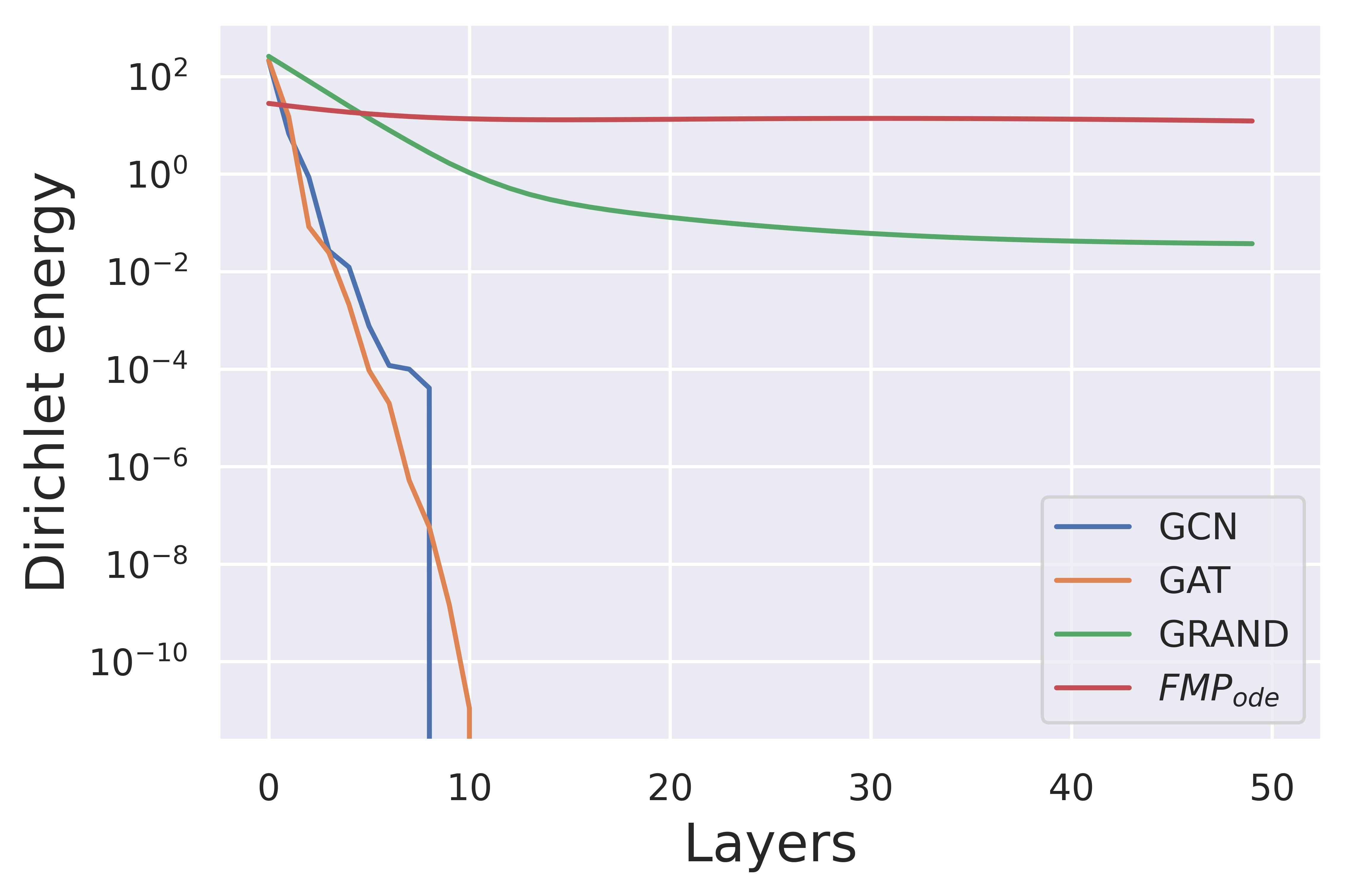
Figure 3: Energy evolution for FMPode.

We first illustrate the evolution of the Dirichlet energy of FMP by an undirected synthetic random graph. The synthetic graph has 100 nodes with two classes and 2D feature which is sampled from the normal distribution with the same standard deviation $\sigma=2$ and two means $\mu_{1}=-0.5,$ $\mu_{2}=0.5.$ The nodes are connected randomly with probability $p=0.9$ if they are in the same class, otherwise nodes in different classes are connected with probability $p=0.1.$ We compare the energy behavior of GNN models with four message passing propagators: GCNs (Kipf and Welling, 2017), GAT (Veličković et al., 2018), GRAND (Chamberlain et al., 2021) and FMPode. We visualize how the node features evolve during $50$ layers of message passing process, from input features at layer $0$ to output features at layer $50$. For each model, the parameters are all properly initialized. The Dirichlet energy of each layer’s output are plotted in logarithm scales. Traditional GNNs such as GCN and GAT suffer oversmoothing as the Dirichlet energy exponentially decays to zero within the first ten layers. GRAND relieves this problem by adding skip connections. FMPode increases energy mildly over network propagation. The oversmoothing issue in GNNs is circumvented with FMPode.

9 Related Work

9.1 Message Passing on Graph Neural Networks

Message Passing Neural Network (MPNN) (Gilmer et al., 2017) establishes a general computational framework of graph feature propagation that covers the majority of update rules for attributed graphs. In each round, every node computes a message and passes the message to its adjacent nodes. Next, a random node aggregates the messages it receives and uses the aggregation to update its embedding. Different graph convolutions vary in the choice of aggregation. For instance, GCN (Kipf and Welling, 2017) and GraphSage Hamilton et al. (2017) operate (selective) summation to neighborhood features, and some other work refines the aggregation weights by the attention mechanism (Xie et al., 2020; Brody et al., 2022) or graph rewiring (Ruiz et al., 2020; Brüel-Gabrielsson et al., 2022; Banerjee et al., 2022; Deac et al., 2022). While constructing propagation rules from the adjacency matrix, i.e., spatial-based graph convolution, is effective enough to encode those relatively-simple graphs instances, it has been demonstrated that such methods ignore high-frequency local information in the input graph signals (Bo et al., 2021). With an increased number of layers, such convolutions only learn node degree and connected components under the influence of the Laplacian spectrum (Oono and Suzuki, 2019), and the non-linear operation merely slows down the convolution speed (Wu et al., 2019).

9.2 Spectral Graph Transforms

Spectral-based graph convolutions have shown promising performance in transferring a trained graph convolution between different graphs, i.e., the model is transferable and generalizable (Levie et al., 2019; Gama et al., 2020). The output of spectral-based methods is stable with respect to perturbations of the input graphs (Ruiz et al., 2021; Zhou et al., 2022; Maskey et al., 2022). In literature, a diverse set of spectral transforms have been applied on graphs, such as Haar (Li et al., 2020; Wang et al., 2020) where Haar convolution and Haar pooling were proposed using the hierarchical Haar bases on a chain of graphs, scattering (Gao et al., 2019; Ioannidis et al., 2020)where the contractive graph scattering wavelets mimic the deep neural networks with wavelets are neurons and the decomposition is the propagation of the layers, needlets (Yi et al., 2022) when the semidiscrete spherical wavelets are used to define approximate equivariance neural networks for sphere data, and framelets (Dong, 2017; Wang and Zhuang, 2019; Zheng et al., 2022) where the spectral graph convolutions are induced by graph framelets.

9.3 Oversmoothness in Graph Representation

As many spatial-based graph convolutions merely perform a low-pass filter that smooths out the local perturbations in the input graph signal, smoothing has been identified as a common phenomenon in MPNNs (Li et al., 2018; Zhao and Akoglu, 2019; Nt and Maehara, 2019). Previous works usually measure and quantify the level of oversmoothing in a graph representation by the distances between node pairs (Rong et al., 2019; Zhao and Akoglu, 2019; Chen et al., 2020a; Hou et al., 2020). When carrying out multiple times of signal smoothing operations, the output of nodes from different clusters tends to converge to similar vectors. While oversmoothing deteriorates the performance in GNNs, efforts have been made to preserve the identity of individual messages by modifying the message passing scheme, such as introducing jump connections (Xu et al., 2018; Chen et al., 2020b), sampling neighboring nodes and edges (Rong et al., 2019; Feng et al., 2020), adding regularizations (Chen et al., 2020a; Zhou et al., 2020; Yang et al., 2021), and increasing the complexity of convolutional layers (Balcilar et al., 2021; Geerts et al., 2021; Bodnar et al., 2021; Wang et al., 2022). Other methods try to trade-off graph smoothness with the fitness of the encoded features (Zhu et al., 2021; Zhou et al., 2021, 2022) or postpone the occurrence of oversmoothing by mechanisms, such as residual networks (Li et al., 2021a; Liu et al., 2021) and the diffusion scheme (Chamberlain et al., 2021; Zhao et al., 2021).

9.4 Stability of Graph Convolutions

While MPNN-based spatial graph convolutions have attracted increasing attentions due to their intuitive architecture and promising performance. However, when the generalization progress is required from a small graph to a larger one, summation-based MPNNs do not show satisfying stability and transferability (Yehudai et al., 2021). In fact, the associated generalization bound from one graph to another is directly proportional to the largest eigenvalue of the graph Laplacian (Verma and Zhang, 2019). Consequently, employing spectral graph filters that are robust to certain structural perturbations becomes a necessary condition for transferability in graph representation learning. Earlier work discussed the linear stability of spectral graph filters in the Cayley smoothness space with respect to the change in the normalized graph Laplacian matrix (Levie et al., 2019; Kenlay et al., 2020; Gama et al., 2020). The stability of graph-based models could be measured by the statistical properties of the model, where the graph topology and signal are viewed as random variables. It has been shown that the output of the spectral filters in stochastic time-evolving graphs behave the same as the deterministic filters in expectation (Isufi et al., 2017). Ceci and Barbarossa (2018) approximated the original filtering process with uncertainties in the graph topology. Later on, stochastic analysis is leveraged to learn graph filters with topological stochasticity (Gao et al., 2021). Maskey et al. (2022) proved the stability of the spatial-based message passing. Kenlay et al. (2020, 2021a, 2021b) proved the stability for the spectral GCNs.

10 Conclusion

This work proposes an expressive framelet message passing for GNN propagation. The framelet coefficients of neighboring nodes provide a graph rewiring scheme to amalgamate features in the framelet domain. We show that our FMP circumvents oversmoothing that appears in most spatial GNN methods. The spectral information reserves extra expressivity to the graph representation by taking multiscale framelet representation into account. Moreover, FMP has good stability in learning node feature representations at low computational complexity.

References

- Balcilar et al. (2021) Muhammet Balcilar, Pierre Héroux, Benoit Gauzere, Pascal Vasseur, Sébastien Adam, and Paul Honeine. Breaking the limits of message passing graph neural networks. In ICML, pages 599–608, 2021.
- Banerjee et al. (2022) Pradeep Kr Banerjee, Kedar Karhadkar, Yu Guang Wang, Uri Alon, and Guido Montúfar. Oversquashing in gnns through the lens of information contraction and graph expansion. In 2022 58th Annual Allerton Conference on Communication, Control, and Computing (Allerton), pages 1–8. IEEE, 2022.
- Beaini et al. (2021) Dominique Beaini, Saro Passaro, Vincent Létourneau, Will Hamilton, Gabriele Corso, and Pietro Liò. Directional graph networks. In ICML, pages 748–758, 2021.
- Bo et al. (2021) Deyu Bo, Xiao Wang, Chuan Shi, and Huawei Shen. Beyond low-frequency information in graph convolutional networks. In AAAI, volume 35, pages 3950–3957, 2021.
- Bodnar et al. (2021) Cristian Bodnar, Fabrizio Frasca, Yuguang Wang, Nina Otter, Guido F Montufar, Pietro Lio, and Michael Bronstein. Weisfeiler and lehman go topological: Message passing simplicial networks. In ICML, pages 1026–1037. PMLR, 2021.
- Brody et al. (2022) Shaked Brody, Uri Alon, and Eran Yahav. How attentive are graph attention networks? In ICLR, 2022.
- Bronstein et al. (2017) Michael M Bronstein, Joan Bruna, Yann LeCun, Arthur Szlam, and Pierre Vandergheynst. Geometric deep learning: going beyond Euclidean data. IEEE Signal Processing Magazine, 34(4):18–42, 2017.
- Brüel-Gabrielsson et al. (2022) Rickard Brüel-Gabrielsson, Mikhail Yurochkin, and Justin Solomon. Rewiring with positional encodings for graph neural networks. arXiv:2201.12674, 2022.
- Cai and Wang (2020) Chen Cai and Yusu Wang. A note on over-smoothing for graph neural networks. In ICML Workshop on Graph Representation Learning, 2020.
- Ceci and Barbarossa (2018) Elena Ceci and Sergio Barbarossa. Robust graph signal processing in the presence of uncertainties on graph topology. 2018 IEEE 19th International Workshop on Signal Processing Advances in Wireless Communications (SPAWC), pages 1–5, 2018.
- Chamberlain et al. (2021) Ben Chamberlain, James Rowbottom, Maria I Gorinova, Michael Bronstein, Stefan Webb, and Emanuele Rossi. Grand: Graph neural diffusion. In ICML, pages 1407–1418. PMLR, 2021.
- Chen et al. (2020a) Deli Chen, Yankai Lin, Wei Li, Peng Li, Jie Zhou, and Xu Sun. Measuring and relieving the over-smoothing problem for graph neural networks from the topological view. In AAAI, volume 34, pages 3438–3445, 2020a.
- Chen et al. (2020b) Ming Chen, Zhewei Wei, Zengfeng Huang, Bolin Ding, and Yaliang Li. Simple and deep graph convolutional networks. In ICML, pages 1725–1735. PMLR, 2020b.
- Daubechies (1992) Ingrid Daubechies. Ten lectures on wavelets, volume 61 of CBMS-NSF Regional Conference Series in Applied Mathematics. Society for Industrial and Applied Mathematics (SIAM),Philadelphia, PA, 1992.
- Deac et al. (2022) Andreea Deac, Marc Lackenby, and Petar Veličković. Expander graph propagation. In The First Learning on Graphs Conference, 2022.
- Dong (2017) Bin Dong. Sparse representation on graphs by tight wavelet frames and applications. Applied and Computational Harmonic Analysis, 42(3):452–479, 2017.
- Dormand and Prince (1980) John R Dormand and Peter J Prince. A family of embedded Runge-Kutta formulae. Journal of Computational and Applied Mathematics, 6(1):19–26, 1980.
- Feng et al. (2020) Wenzheng Feng, Jie Zhang, Yuxiao Dong, Yu Han, Huanbo Luan, Qian Xu, Qiang Yang, Evgeny Kharlamov, and Jie Tang. Graph random neural networks for semi-supervised learning on graphs. NeurIPS, 33:22092–22103, 2020.
- Gama et al. (2020) Fernando Gama, Joan Bruna, and Alejandro Ribeiro. Stability properties of graph neural networks. IEEE Transactions on Signal Processing, 68:5680–5695, 2020.
- Gao et al. (2019) Feng Gao, Guy Wolf, and Matthew Hirn. Geometric scattering for graph data analysis. In ICML, pages 2122–2131. PMLR, 2019.
- Gao et al. (2021) Zhan Gao, Elvin Isufi, and Alejandro Ribeiro. Stochastic graph neural networks. IEEE Transactions on Signal Processing, 69:4428–4443, 2021.
- García-Plaza et al. (2016) Alberto P García-Plaza, Víctor Fresno, Raquel Martínez Unanue, and Arkaitz Zubiaga. Using fuzzy logic to leverage html markup for web page representation. IEEE Transactions on Fuzzy Systems, 25(4):919–933, 2016.
- Gasteiger et al. (2018) Johannes Gasteiger, Aleksandar Bojchevski, and Stephan Günnemann. Predict then propagate: Graph neural networks meet personalized pagerank. In ICLR, 2018.
- Geerts et al. (2021) Floris Geerts, Filip Mazowiecki, and Guillermo Perez. Let’s agree to degree: Comparing graph convolutional networks in the message-passing framework. In ICML, pages 3640–3649. PMLR, 2021.
- Gilmer et al. (2017) Justin Gilmer, Samuel S Schoenholz, Patrick F Riley, Oriol Vinyals, and George E Dahl. Neural message passing for quantum chemistry. In ICML, 2017.
- Hamilton (2020) William L Hamilton. Graph representation learning. Synthesis Lectures on Artifical Intelligence and Machine Learning, 14(3):1–159, 2020.
- Hamilton et al. (2017) William L Hamilton, Rex Ying, and Jure Leskovec. Inductive representation learning on large graphs. In NIPS, 2017.
- Hou et al. (2020) Yifan Hou, Jian Zhang, James Cheng, Kaili Ma, Richard T. B. Ma, Hongzhi Chen, and Ming Yang. Measuring and improving the use of graph information in graph neural networks. arXiv:2206.13170, 2020.
- Ioannidis et al. (2020) Vassilis N Ioannidis, Siheng Chen, and Georgios B Giannakis. Pruned graph scattering transforms. In ICLR, 2020.
- Isufi et al. (2017) Elvin Isufi, Andreas Loukas, Andrea Simonetto, and Geert Leus. Filtering random graph processes over random time-varying graphs. IEEE Transactions on Signal Processing, 65(16):4406–4421, 2017.
- Kenlay et al. (2020) Henry Kenlay, Dorina Thanou, and Xiaowen Dong. On the stability of polynomial spectral graph filters. In ICASSP 2020-2020 IEEE International Conference on Acoustics, Speech and Signal Processing (ICASSP), pages 5350–5354. IEEE, 2020.
- Kenlay et al. (2021a) Henry Kenlay, Dorina Thano, and Xiaowen Dong. On the stability of graph convolutional neural networks under edge rewiring. In ICASSP 2021-2021 IEEE International Conference on Acoustics, Speech and Signal Processing (ICASSP), pages 8513–8517. IEEE, 2021a.
- Kenlay et al. (2021b) Henry Kenlay, Dorina Thanou, and Xiaowen Dong. Interpretable stability bounds for spectral graph filters. In Marina Meila and Tong Zhang, editors, ICML, volume 139 of PMLR, pages 5388–5397. PMLR, 18–24 Jul 2021b.
- Kipf and Welling (2017) Thomas N. Kipf and Max Welling. Semi-supervised classification with graph convolutional networks. In ICLR, 2017.
- Levie et al. (2019) Ron Levie, Elvin Isufi, and Gitta Kutyniok. On the transferability of spectral graph filters. In 2019 13th International conference on Sampling Theory and Applications (SampTA), pages 1–5. IEEE, 2019.
- Li et al. (2021a) Guohao Li, Matthias Müller, Bernard Ghanem, and Vladlen Koltun. Training graph neural networks with 1000 layers. In ICML, pages 6437–6449. PMLR, 2021a.
- Li et al. (2020) Ming Li, Zheng Ma, Yu Guang Wang, and Xiaosheng Zhuang. Fast haar transforms for graph neural networks. Neural Networks, 128:188–198, 2020.
- Li et al. (2018) Qimai Li, Zhichao Han, and Xiao-Ming Wu. Deeper insights into graph convolutional networks for semi-supervised learning. In Thirty-Second AAAI conference on artificial intelligence, 2018.
- Li et al. (2021b) Shouheng Li, Dongwoo Kim, and Qing Wang. Beyond low-pass filters: Adaptive feature propagation on graphs. In Machine Learning and Knowledge Discovery in Databases. Research Track: European Conference, ECML PKDD 2021, Bilbao, Spain, September 13–17, 2021, Proceedings, Part II 21, pages 450–465. Springer, 2021b.
- Liu et al. (2021) Xiaorui Liu, Jiayuan Ding, Wei Jin, Han Xu, Yao Ma, Zitao Liu, and Jiliang Tang. Graph neural networks with adaptive residual. NeurIPS, 34:9720–9733, 2021.
- Maskey et al. (2022) Sohir Maskey, Ron Levie, Yunseok Lee, and Gitta Kutyniok. Generalization analysis of message passing neural networks on large random graphs. In NeurIPS, 2022.
- Nt and Maehara (2019) Hoang Nt and Takanori Maehara. Revisiting graph neural networks: All we have is low-pass filters. arXiv:1905.09550, 2019.
- Oono and Suzuki (2019) Kenta Oono and Taiji Suzuki. Graph neural networks exponentially lose expressive power for node classification. In ICLR, 2019.
- Pei et al. (2019) Hongbin Pei, Bingzhe Wei, Kevin Chen-Chuan Chang, Yu Lei, and Bo Yang. Geom-gcn: Geometric graph convolutional networks. In ICLR, 2019.
- Poli et al. (2019) Michael Poli, Stefano Massaroli, Junyoung Park, Atsushi Yamashita, Hajime Asama, and Jinkyoo Park. Graph neural ordinary differential equations. arXiv:1911.07532, 2019.
- Rong et al. (2019) Yu Rong, Wenbing Huang, Tingyang Xu, and Junzhou Huang. Dropedge: Towards deep graph convolutional networks on node classification. arXiv:1907.10903, 2019.
- Ruiz et al. (2020) Luana Ruiz, Luiz Chamon, and Alejandro Ribeiro. Graphon neural networks and the transferability of graph neural networks. NeurIPS, 33:1702–1712, 2020.
- Ruiz et al. (2021) Luana Ruiz, Fernando Gama, and Alejandro Ribeiro. Graph neural networks: architectures, stability, and transferability. Proceedings of the IEEE, 109(5):660–682, 2021.
- Stachenfeld et al. (2020) Kimberly Stachenfeld, Jonathan Godwin, and Peter Battaglia. Graph networks with spectral message passing. In NeurIPS 2020 Workshop on Interpretable Inductive Biases and Physically Structured Learning, 2020.
- Stein and Shakarchi (2011) Elias M Stein and Rami Shakarchi. Fourier Analysis: an Introduction, volume 1. Princeton University Press, 2011.
- Veličković et al. (2018) Petar Veličković, Guillem Cucurull, Arantxa Casanova, Adriana Romero, Pietro Liò, and Yoshua Bengio. Graph attention networks. In ICLR, 2018.
- Verma and Zhang (2019) Saurabh Verma and Zhi-Li Zhang. Stability and generalization of graph convolutional neural networks. In Proceedings of the 25th ACM SIGKDD International Conference on Knowledge Discovery & Data Mining, pages 1539–1548, 2019.
- Wang and Zhuang (2019) Yu Guang Wang and Xiaosheng Zhuang. Tight framelets on graphs for multiscale data analysis. In Wavelets and Sparsity XVIII, volume 11138, page 111380B. International Society for Optics and Photonics, 2019.
- Wang et al. (2020) Yu Guang Wang, Ming Li, Zheng Ma, Guido Montufar, Xiaosheng Zhuang, and Yanan Fan. Haar graph pooling. In ICML, pages 9952–9962. PMLR, 2020.
- Wang et al. (2022) Yuelin Wang, Kai Yi, Xinliang Liu, Yu Guang Wang, and Shi Jin. Acmp: Allen-cahn message passing for graph neural networks with particle phase transition. arXiv:2206.05437, 2022.
- Wu et al. (2019) Felix Wu, Amauri Souza, Tianyi Zhang, Christopher Fifty, Tao Yu, and Kilian Weinberger. Simplifying graph convolutional networks. In ICML, 2019.
- Wu et al. (2020) Zonghan Wu, Shirui Pan, Fengwen Chen, Guodong Long, Chengqi Zhang, and S Yu Philip. A comprehensive survey on graph neural networks. IEEE TNNLS, 32(1):4–24, 2020.
- Xhonneux et al. (2020) Louis-Pascal Xhonneux, Meng Qu, and Jian Tang. Continuous graph neural networks. In International Conference on Machine Learning, pages 10432–10441. PMLR, 2020.
- Xie et al. (2020) Yu Xie, Yuanqiao Zhang, Maoguo Gong, Zedong Tang, and Chao Han. Mgat: Multi-view graph attention networks. Neural Networks, 132:180–189, 2020.
- Xu et al. (2018) Keyulu Xu, Chengtao Li, Yonglong Tian, Tomohiro Sonobe, Ken-ichi Kawarabayashi, and Stefanie Jegelka. Representation learning on graphs with jumping knowledge networks. In ICML, 2018.
- Xu et al. (2019) Keyulu Xu, Weihua Hu, Jure Leskovec, and Stefanie Jegelka. How powerful are graph neural networks? In ICLR, 2019.
- Yang et al. (2021) Yongyi Yang, Tang Liu, Yangkun Wang, Jinjing Zhou, Quan Gan, Zhewei Wei, Zheng Zhang, Zengfeng Huang, and David Wipf. Graph neural networks inspired by classical iterative algorithms. In ICML, pages 11773–11783. PMLR, 2021.
- Yang et al. (2016) Zhilin Yang, William Cohen, and Ruslan Salakhudinov. Revisiting semi-supervised learning with graph embeddings. In ICML, 2016.
- Yehudai et al. (2021) Gilad Yehudai, Ethan Fetaya, Eli Meirom, Gal Chechik, and Haggai Maron. From local structures to size generalization in graph neural networks. In ICML, pages 11975–11986. PMLR, 2021.
- Yi et al. (2022) Kai Yi, Jialin Chen, Yu Guang Wang, Bingxin Zhou, Pietro Liò, Yanan Fan, and Jan Hamann. Approximate equivariance so (3) needlet convolution. In Topological, Algebraic and Geometric Learning Workshops 2022, pages 189–198. PMLR, 2022.
- Zhao et al. (2021) Jialin Zhao, Yuxiao Dong, Ming Ding, Evgeny Kharlamov, and Jie Tang. Adaptive diffusion in graph neural networks. Advances in Neural Information Processing Systems, 34:23321–23333, 2021.
- Zhao and Akoglu (2019) Lingxiao Zhao and Leman Akoglu. Pairnorm: Tackling oversmoothing in gnns. In ICLR, 2019.
- Zheng et al. (2021) Xuebin Zheng, Bingxin Zhou, Junbin Gao, Yu Guang Wang, Pietro Lio, Ming Li, and Guido Montúfar. How framelets enhance graph neural networks. In ICML, 2021.
- Zheng et al. (2022) Xuebin Zheng, Bingxin Zhou, Yu Guang Wang, and Xiaosheng Zhuang. Decimated framelet system on graphs and fast g-framelet transforms. Journal of Machine Learning Research, 23(18):1–68, 2022.
- Zhou et al. (2021) Bingxin Zhou, Ruikun Li, Xuebin Zheng, Yu Guang Wang, and Junbin Gao. Graph denoising with framelet regularizer. arXiv:2111.03264, 2021.
- Zhou et al. (2022) Bingxin Zhou, Yuanhong Jiang, Yu Guang Wang, Jingwei Liang, Junbin Gao, Shirui Pan, and Xiaoqun Zhang. Robust graph representation learning for local corruption recovery. ICML Workshop on Topology, Algebra, and Geometry in Machine Learning (TAG-ML), 2022.
- Zhou (2014) Houqing Zhou. On some trace inequalities for positive definite hermitian matrices. Journal of Inequalities and Applications, 2014(1):1–6, 2014.
- Zhou et al. (2020) Kaixiong Zhou, Xiao Huang, Yuening Li, Daochen Zha, Rui Chen, and Xia Hu. Towards deeper graph neural networks with differentiable group normalization. NeurIPS, 33:4917–4928, 2020.
- Zhu et al. (2020) Jiong Zhu, Yujun Yan, Lingxiao Zhao, Mark Heimann, Leman Akoglu, and Danai Koutra. Beyond homophily in graph neural networks: Current limitations and effective designs. Advances in Neural Information Processing Systems, 33:7793–7804, 2020.
- Zhu et al. (2021) Meiqi Zhu, Xiao Wang, Chuan Shi, Houye Ji, and Peng Cui. Interpreting and unifying graph neural networks with an optimization framework. In Proceedings of the Web Conference, pages 1215–1226, 2021.