The JCMT Nearby Galaxies Legacy Survey: SCUBA-2 observations of nearby galaxies

Abstract

We present 850$\mu$m observations of a sample of 8 nearby spiral galaxies, made using the SCUBA-2 camera on the James Clerk Maxwell Telescope (JCMT) as part of the JCMT Nearby Galaxies Legacy Survey (NGLS). We corrected our data for the presence of the ¹²CO $J=3\to 2$ line in the SCUBA-2 850$\mu$m bandwidth using NGLS HARP data, finding a typical ¹²CO contribution of $\sim 20$%. We measured dust column densities, temperatures and opacity indices by fitting spectral energy distributions constructed from SCUBA-2 and archival Herschel observations, and used archival GALEX and Spitzer data to make maps of surface density of star formation ($\Sigma_{\textsc{sfr}}$). Typically, comparing SCUBA-2-derived H₂ surface densities ($\Sigma_{\rm H_{2}}$) to $\Sigma_{\textsc{sfr}}$ gives shallow star formation law indices within galaxies, with SCUBA-2-derived values typically being sublinear and Herschel-derived values typically being broadly linear. This difference is likely due to the effects of atmospheric filtering on the SCUBA-2 data. Comparing the mean values of $\Sigma_{\rm H_{2}}$ and $\Sigma_{\textsc{sfr}}$ of the galaxies in our sample returns a steeper star formation law index, broadly consistent with both the Kennicutt-Schmidt value of 1.4 and linearity. Our results show that a SCUBA-2 detection is a good predictor of star formation. We suggest that Herschel emission traces gas in regions which will form stars on timescales $\sim 5-100$ Myr, comparable to the star formation timescale traced by GALEX and Spitzer data, while SCUBA-2 preferentially traces the densest gas within these regions, which likely forms stars on shorter timescales.

1 Introduction

The evolution of a galaxy is intrinsically linked to the star formation that takes place within it. Stars form from the densest phase of the interstellar medium of galaxies, from gravitationally unstable structures within clouds composed primarily of dense molecular hydrogen (Bergin & Tafalla, 2007). Understanding the timescale on which, and efficiency with which, molecular gas is converted into stars is crucial to understanding the star-forming histories of galaxies (e.g. Kennicutt & Evans, 2012).

One of the key metrics by which the link between the gas properties of galaxies and the star formation within them is parametrized is the Kennicutt-Schmidt (KS) star formation law (Schmidt, 1959; Kennicutt, 1998), a scaling relation between surface gas density ($\Sigma_{gas}$) and surface density of star formation rate ($\Sigma_{\textsc{sfr}}$). The star formation law can be measured either between a sample of galaxies (e.g. Kennicutt, 1998) or within individual galaxies (e.g. Leroy et al., 2008). $\Sigma_{\textsc{sfr}}$ is typically well-correlated with $\Sigma_{gas}$, and the relationship is parametrized as

$$\Sigma_{\textsc{sfr}}\propto\Sigma_{gas}^{N}$$ (1)

(Schmidt, 1959; Kennicutt, 1998). Kennicutt (1998) found $N=1.4\pm 0.15$, measuring disc-averaged values of both quantities over an ensemble of galaxies. However, the molecular gas surface density ($\Sigma_{{\rm H}_{2}}$) is typically much better-correlated with $\Sigma_{\textsc{sfr}}$ than is the total gas surface density (Wong & Blitz, 2002), as might be expected given that star formation occurs within clouds of cold molecular gas (e.g. Kennicutt & Evans, 2012).

The relationship between $\Sigma_{SFR}$ and $\Sigma_{gas}$ or $\Sigma_{{\rm H}_{2}}$ within individual galaxies (the resolved KS law) has also been extensively investigated (e.g. Bigiel et al., 2008; Bolatto et al., 2017; Zabel et al., 2020; Ellison et al., 2021). On scales $\gtrsim 1\,$kpc, a correlation is seen between $\Sigma_{SFR}$ and $\Sigma_{{\rm H}_{2}}$; Bigiel et al. (2008) found an average index $N=1.0\pm 0.2$ between $\Sigma_{{\rm H}_{2}}$ and $\Sigma_{SFR}$ in a sample of spiral galaxies. This linear relationship, also found by Bolatto et al. (2017), suggests that stars form from molecular gas with constant efficiency within these galaxies. The offset of the resolved KS law varies significantly between galaxies, with galaxies with higher stellar masses, larger Sersic indices, and lower specific star formation rates typically having a lower resolved KS law (Ellison et al., 2021). Moreover, a range of values of $N$ have been found in nearby galaxies: for example, Ford et al. (2013), observing M31, found a super-KS index of $2.03\pm 0.04$ for $\Sigma_{gas}$ (Hi, and H₂ from CO), but sublinear indices for molecular gas only: $0.60\pm 0.01$ for $\Sigma_{{\rm H}_{2}}$ from CO, and $0.55\pm 0.01$ for $\Sigma_{{\rm H}_{2}}$ from Herschel dust emission, assuming a radial gas-to-dust ratio gradient. A sub-linear star formation law suggests that star formation becomes less efficient at high gas densities, which is difficult to physically motivate. However, Williams et al. (2018), observing M33, found on kpc scales an index $1.30\pm 0.11$ for molecular gas from CO, but $5.53\pm 0.75$ for total gas and $5.85\pm 2.37$ for gas from dust, with all three quantities varying significantly with the spatial scale over which they were measured. These differences are likely due to the disc of M33 being Hi-dominated (Williams et al., 2018); surface density of atomic gas $\Sigma_{{\rm H}\textsc{i}}$ is a poor tracer of $\Sigma_{SFR}$ (e.g. Gao & Solomon, 2004). The index measured also depends on the amount of diffuse background subtracted in both the gas and the star formation rate tracers (Kumari et al., 2020).

Molecular clouds contain an interstellar dust component, consisting principally of silicates, carbonaceous grains, and polyaromatic hydrocarbons (PAHs), which typically makes up $\sim 1$% of molecular clouds by mass (e.g. Draine & Li, 2007). Continuum emission from interstellar dust is a widely-used tracer of molecular gas (e.g. Hildebrand, 1983). The James Clerk Maxwell Telescope (JCMT) Nearby Galaxies Legacy Survey (NGLS, Wilson et al., 2009, 2012) is a large programme which mapped the molecular gas and dust in a sample of galaxies within a distance of 25 Mpc. In this paper, we present Submillimetre Common-User Bolometer Array 2 (SCUBA-2) 850$\mu$m dust emission observations of 8 galaxies from the NGLS sample.

We present the observations in Section 2, and briefly review the galaxies which we consider in Section 3. In Section 4 we compare the dust and atomic and molecular gas distributions of the galaxies which we consider. In Section 5 we describe the process of fitting modified black-body functions to the spectral energy distributions of the galaxies which we consider. In Section 6 we construct resolved and unresolved star formation laws for the galaxies which we consider. In Section 7 we discuss our results. Section 8 summarises this work.

2 Observations

	R.A.	Dec.	Hubble		Distance
Galaxy	(J2000)	(J2000)	classification	Inclination	(Mpc)	$12+\log_{10}({\rm O/H})$
NGC 3034	$09^{h}55^{m}52\aas@@fstack{\prime\prime}43$	$+69^{\circ}40^{\prime}46\aas@@fstack{\prime\prime}9$	Scd	76.9	3.61	–
NGC 3351	$10^{h}43^{m}57\aas@@fstack{s}73$	$+11^{\circ}42^{\prime}13\aas@@fstack{\prime\prime}0$	Sb	54.6	9.91	$8.654^{+0.018}_{-0.020}$
NGC 3521	$11^{h}05^{m}48\aas@@fstack{s}57$	$-00^{\circ}02^{\prime}09\aas@@fstack{\prime\prime}2$	SABb	60.0	12.42	$8.604^{+0.026}_{-0.027}$
NGC 4254	$12^{h}18^{m}49\aas@@fstack{s}63$	$+14^{\circ}24^{\prime}59\aas@@fstack{\prime\prime}4$	Sc	20.1	12.88	$8.554^{+0.020}_{-0.021}$
NGC 4569	$12^{h}36^{m}49\aas@@fstack{s}82$	$+13^{\circ}09^{\prime}46\aas@@fstack{\prime\prime}3$	SABa	70.8	11.86	–
NGC 4736	$12^{h}50^{m}53\aas@@fstack{s}15$	$+41^{\circ}07^{\prime}12\aas@@fstack{\prime\prime}6$	Sab	31.7	4.39	$8.623^{+0.046}_{-0.046}$
NGC 5055	$13^{h}15^{m}49\aas@@fstack{s}27$	$+42^{\circ}01^{\prime}45\aas@@fstack{\prime\prime}7$	Sbc	54.9	9.04	$8.581^{+0.054}_{-0.053}$
NGC 5194	$13^{h}29^{m}52\aas@@fstack{s}70$	$+47^{\circ}11^{\prime}42\aas@@fstack{\prime\prime}9$	Sbc	32.6	8.59	$8.638^{+0.012}_{-0.006}$

Table 1: The coordinates, Hubble classifications, inclinations, distances and metallicities of our set of galaxies. Classifications, inclinations, distances and metallicities (where present) are taken from the Dustpedia database (Clark et al., 2018). Dustpedia metallicities are presented by De Vis et al. (2019); we use their preferred ‘PG16S’ calibration. We compare these to a solar metallicity of $12+\log_{10}({\rm O/H})=8.69\pm 0.05$ (Asplund et al., 2009).

The SCUBA-2 850$\mu$m data presented in this paper was taken under project code MJLSN07. All data were taken using the SCUBA-2 CV-DAISY mapping mode, with the exception of NGC 5194, which was mapped using the PONG-900 mode (Holland et al., 2013). The CV-DAISY mode was used for these extended sources despite being optimised for compact sources because it produces a high exposure time in the map centre, which is necessary to observe relatively small low-surface-brightness sources in a reasonable amount of time (Holland et al., 2013).

We selected 8 bright galaxies (listed in Table 1) with ancillary observations of the ¹²CO $J=1\to 0$ line made using the Nobeyama 45m telescope as part of the COMING (Sorai et al., 2019) and CO-ATLAS (Kuno et al., 2007) surveys. All of the galaxies in our sample were observed in the ¹²CO $J=3\to 2$ line using HARP (Buckle et al., 2009) as part of the NGLS. These galaxies also have ancillary observations with Herschel, GALEX and Spitzer (Clark et al., 2018). These galaxies were selected for submillimetre brightness and completeness of ancillary data sets, and are not intended to be a representative sample of nearby galaxies. The UT start and end dates of the observations, the number of repeats and integration time per source, and the weather conditions under which they were observed are listed in Table 2. These data were largely taken in JCMT weather bands 2 and 3. JCMT weather bands are defined by atmospheric opacity at 225 GHz ($\tau_{225}$); Band 2 is defined by $0.05<\tau_{225}<0.08$, and Band 3 by $0.08<\tau_{225}<0.12$ (Dempsey et al., 2013).

2.1 SCUBA-2 data reduction

We reduced the data using the skyloop implementation of the makemap algorithm in Smurf (Chapin et al., 2013), in which one iteration of makemap is performed on each of the observations in the set in turn, with the set being averaged together at the end of each iteration, rather than each observation being reduced consecutively. Although SCUBA-2 observes 850$\mu$m and 450$\mu$m simultaneously, we consider only 850$\mu$m data in this paper.

In order to ensure good image fidelity, we ran makemap to a tolerance of 1%. We also defined a maximum observable size scale of 180^′′, in order to prevent the growth of large-scale, low-level emission structures in the output map. This maximum size scale is chosen to match the size of the central region of a CV-DAISY map over which exposure times are relatively uniform (Holland et al., 2013), and is more stringent than is usual for SCUBA-2 observations. The default maximum observable size scale is 300^′′, set by the size of a SCUBA-2 subarray (see, e.g., Holland et al. 2013; Kirk et al. 2018). By choosing a smaller maximum size scale, we place stronger constraints on the iterative makemap algorithm, which is necessary in order to accurately recover faint extended sources, particularly when using the CV-DAISY mapping mode, which has a small map size and a non-uniform exposure time.

We used the Nobeyama 45m ¹²CO $J=1\to 0$ maps (Kuno et al., 2007; Sorai et al., 2019) to define a fixed ‘mask’ for each observation, defining areas of astrophysical emission. These observations were chosen because their resolution ($\sim 17^{\prime\prime}$; Sorai et al. 2019) is comparable to that of the JCMT, while their low-$J$ transition and more transmissive atmospheric window give better sensitivity to extended emission over a larger area than do the NGLS HARP $J=3\to 2$ data. Our aim in choosing a mask is to define the maximum area over which dust emission is likely to be detected; we want to provide sufficient constraint on the mapmaker to exclude regions without real signal whilst including an area sufficiently large to allow real extended structure to grow. The masked area was defined by an SNR $>4$ in integrated intensity in the Nobeyama 45m data, as provided by the CO-ATLAS and COMING archives. Areas outside this masked region were set to zero until the final iteration of makemap (see Mairs et al. 2015 for a detailed discussion of the role of masking in SCUBA-2 data reduction). In each case, the SCUBA-2 flux recovered in the output map did not fill the area defined by the mask, indicating that our choice of mask did not encourage the growth of spurious structures in the SCUBA-2 maps.

By choosing these map-making parameters, it is likely that we have sacrificed some potentially-recoverable large-scale structure in order to achieve good image fidelity. We discuss the implications of this choice at various points throughout this work.

The output maps were gridded to 4^′′ pixels and calibrated in mJy beam^-1 and mJy arcsec^-2 using the standard SCUBA-2 850$\mu$m flux conversion factors (FCFs) of 537 Jy beam^-1 pW^-1 and 2340 mJy arcsec^-2 pW^-1 (Dempsey et al., 2013).

The effective resolution of SCUBA-2 at 850$\mu$m is $14\aas@@fstack{\prime\prime}1$. The RMS noise in our maps is in the range 2.6–4.0 mJy beam^-1, with variation between maps being due to differences in exposure time, elevation, and amounts of large-scale structure present. RMS noise values and linear resolutions for each individual field are listed in Table 3.

	UT date			Integration	$\tau_{225}$
Galaxy	Start	End	Repeats	time (mins)	Start	End
NGC 3034	2012 Apr 01	2014 Feb 20	8	$\sim 21$	0.055	0.099
NGC 3351	2014 Feb 12	2014 May 30	8	$\sim 21$	0.098	0.071
NGC 3521	2013 Dec 05	2014 May 30	8	$\sim 21$	0.126	0.074
NGC 4254	2012 Mar 31	2014 Jun 05	11	$\sim 21$	0.054	0.121
NGC 4569	2012 Mar 31	2014 Jun 08	11	$\sim 21$	0.037	0.119
NGC 4736	2012 Feb 04	2014 May 31	11	$\sim 21$	0.086	0.083
NGC 5055	2013 Dec 11	2014 May 29	16	$\sim 21$	0.138	0.111
NGC 5194	2014 Jan 15	2014 May 22	16	$\sim 42$	0.092	0.117

Table 2: Details of the observing dates and conditions for the galaxies in our sample. Note that integration time is given per repeat.

2.2 CO subtraction

	Linear	RMS noise		Peak 850$\mu$m F.D.		Total 850$\mu$m F.D.		Net CO
	resolution	CO-sub		With CO	CO-sub	With CO	CO-sub	fraction
	kpc	mJy beam-1	mJy arcsec-2	mJy arcsec-2		Jy
NGC 3034	0.25	3.7	0.016	6.53	4.45	8.72	5.43	0.38
NGC 3351	0.68	3.4	0.015	0.38	0.27	0.19	0.15	0.19
NGC 3521	0.85	4.0	0.017	0.20	0.18	1.48	1.20	0.18
NGC 4254	0.88	3.8	0.017	0.22	0.16	1.02	0.80	0.21
NGC 4569	0.81	3.8	0.017	0.31	0.22	0.38	0.31	0.17
NGC 4736	0.30	3.0	0.013	0.21	0.14	0.76	0.58	0.24
NGC 5055	0.62	2.6	0.011	0.36	0.28	1.92	1.65	0.14
NGC 5194	0.59	3.3	0.014	0.30	0.21	0.50*	0.24*	0.52

Table 3: The key properties of the SCUBA-2 850$\mu$m measurements of the sources in our sample. The RMS noises listed in this table are measured in the CO-subtracted maps used for analysis. *Note that these values include summation over the significant negative bowls in the interarm regions of NGC 5194.

The SCUBA-2 850$\mu$m filter has a half-power bandwidth of 85$\mu$m (Holland et al., 2013), and so SCUBA-2 850$\mu$m data can include a significant contribution from the ¹²CO $J=3\to 2$ transition, the rest wavelength of which is 867.6$\mu$m (345.8 GHz).

We accounted for the contribution of CO to our SCUBA-2 flux densities using the technique described by Drabek et al. (2012). Each of the 850$\mu$m observations was re-reduced with the integrated HARP (Buckle et al., 2009) ¹²CO data added to the SCUBA-2 bolometer time series as a negative signal. By repeating the data reduction process described in Section 2.1, the same spatial filtering is applied to the subtracted HARP ¹²CO signal as to the SCUBA-2 data, and so the spatial scales in the two data sets are matched. The SCUBA-2 850$\mu$m and HARP ¹²CO data have very similar angular resolutions, agreeing to within 2%, and so no correction for this small difference is necessary.

We used the integrated NGLS HARP ¹²CO maps (Wilson et al., 2012), in which data are supplied for pixels with a SNR $>2$ in total integrated intensity. The conversion from K km s^-1 to pW is dependent on atmospheric opacity; we calculated a conversion factor for each observation from the mean of its start- and end-time 225 GHz opacities using the relations given by Parsons et al. (2018).

For the galaxies in question, the net contribution of ¹²CO to the SCUBA-2 850$\mu$m flux is typically $\sim 20$%, but reaches 38% in NGC 3034 and $\sim 50$% in NGC 5194, although our data reduction strategy in NGC 5194 may be suboptimal, as discussed in Section 3.8, below. The peak and total flux densities before and after CO subtraction are listed in Table 3. CO fractions of order tens of percent in bright regions indicate that this correction cannot be neglected when calculating dust masses from SCUBA-2 observations.

As can be seen in Figures 1–8, the CO contamination fraction drops to near zero at the peripheries of the ¹²CO SNR $>2$ regions, indicating that little or no ¹²CO emission has been retained in the 850$\mu$m images by excluding the lower-SNR data. With the exception of NGC 5194, the area over which SCUBA-2 signal is detected is well-covered by the footprint of the HARP observations. However, in the NGC 5194 field, the companion galaxy, NGC 5195, and a small part of the southern spiral arm of NGC 5194, are not mapped by HARP. The relatively few pixels which are thus bright in 850$\mu$m emission but not corrected for ¹²CO contamination transpire not to be well-characterised and are excluded by data quality cuts discussed later in this work, and so do not affect our conclusions.

We note that much lower CO contamination fractions have been found in SCUBA-2 images of M31 (Smith et al., 2021). The differences in CO fraction between M31 and the galaxies in our sample are likely due to CO emission from M31 having low surface brightness, with line fluxes $<10$ K km s^-1 everywhere (Smith et al., 2021). The galaxies in our sample have significantly higher CO brightnesses (cf. Figures 1–8). As a potential green valley galaxy (Mutch et al., 2011), M31 is likely to have both less gas and less dust than actively star-forming galaxies. There may also be differences in metallicity between the galaxies in our sample and M31. The contribution of ¹²CO $J=3\to 2$ to SCUBA-2 850$\mu$m emission in local Milky Way star-forming regions is typically $\lesssim 20$%, but may be higher in the presence of outflows (Drabek et al., 2012; Pattle et al., 2015; Coudé et al., 2016).

3 Galaxies under consideration

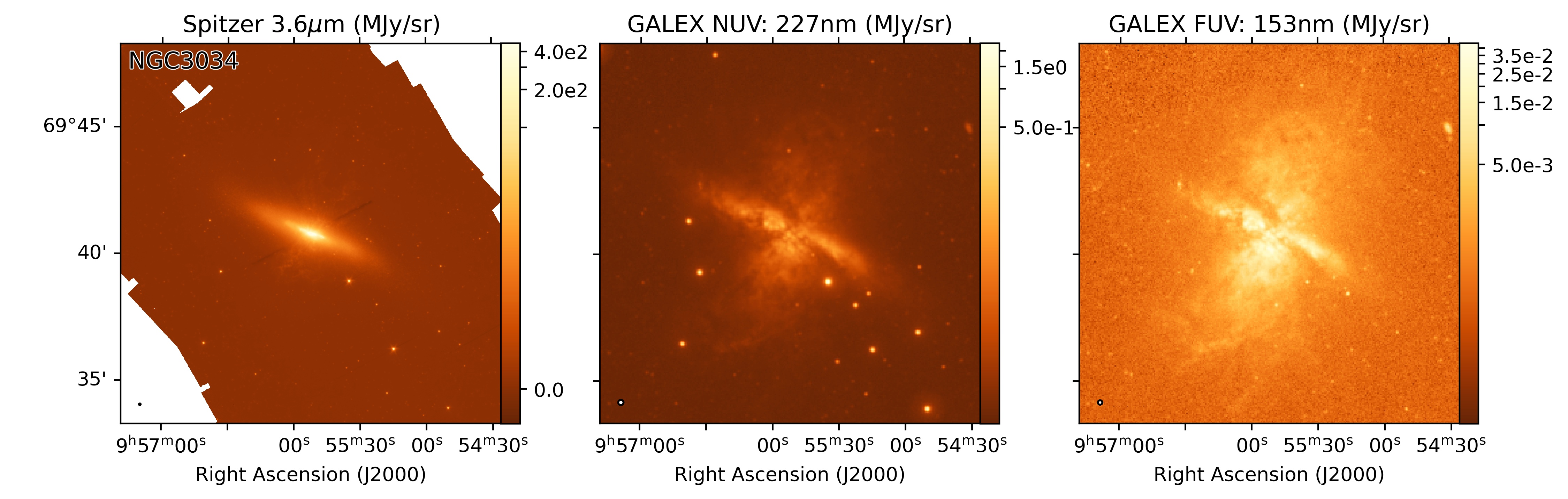
Figure 29: Multiwavelength observations of NGC3034, taken from the Dustpedia database (Clark et al., 2018). Left: Spitzer 3.6 $\mu$m emission. Centre: GALEX NUV emission. Right: GALEX FUV emission. Beam sizes are shown in the lower left-hand corner of each image.

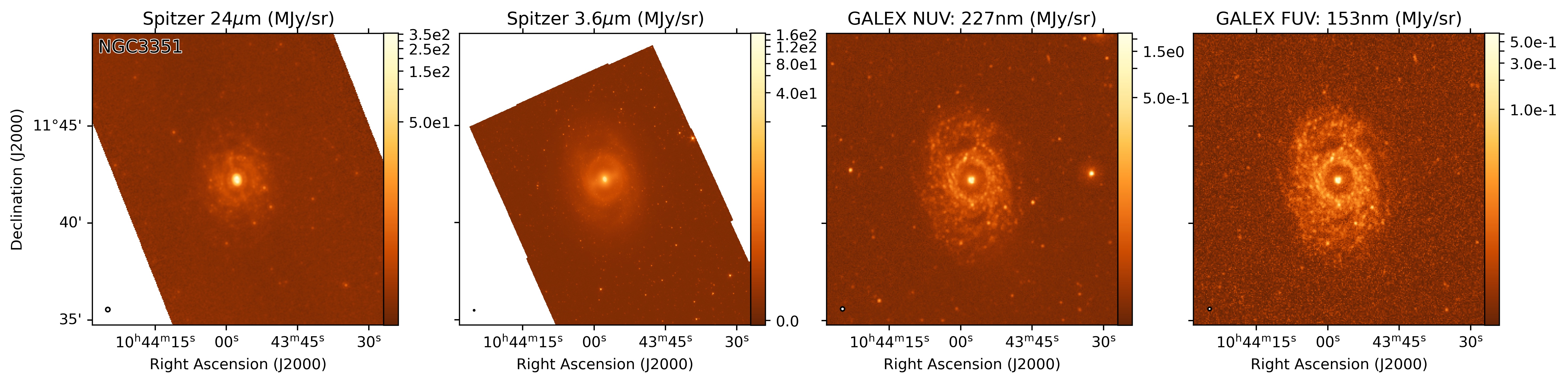
Figure 30: Multiwavelength observations of NGC3351, taken from the Dustpedia database (Clark et al., 2018). Far left: Spitzer 24 $\mu$m emission. Centre left: Spitzer 3.6 $\mu$m emission. Centre right: GALEX NUV emission. Far right: GALEX FUV emission. Beam sizes are shown in the lower left-hand corner of each image.

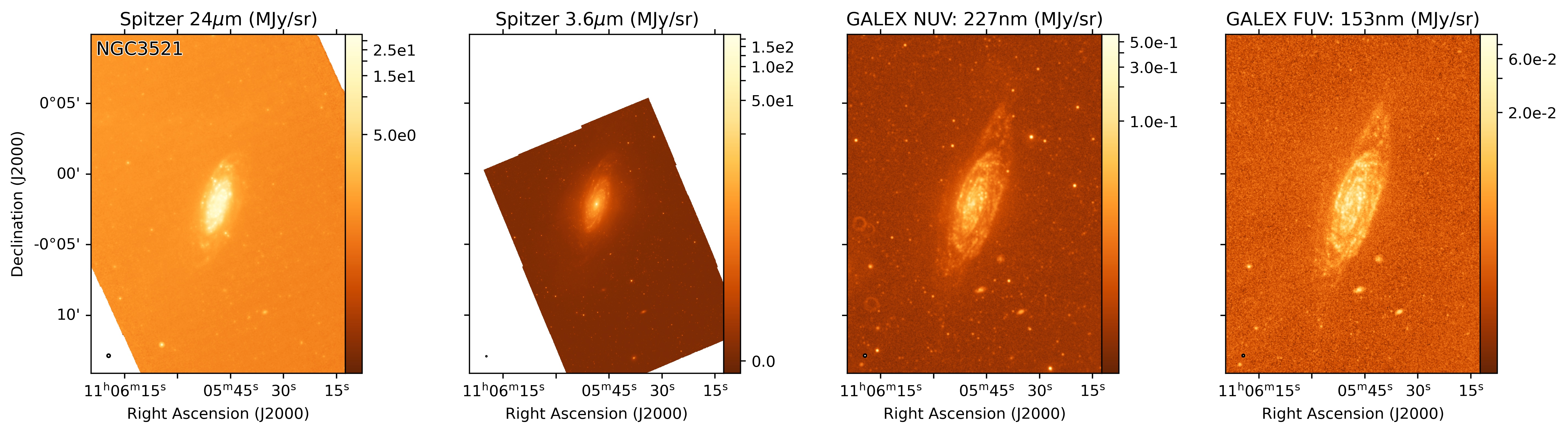
Figure 31: Multiwavelength observations of NGC3521, taken from the Dustpedia database (Clark et al., 2018). Panels as in Figure 30.

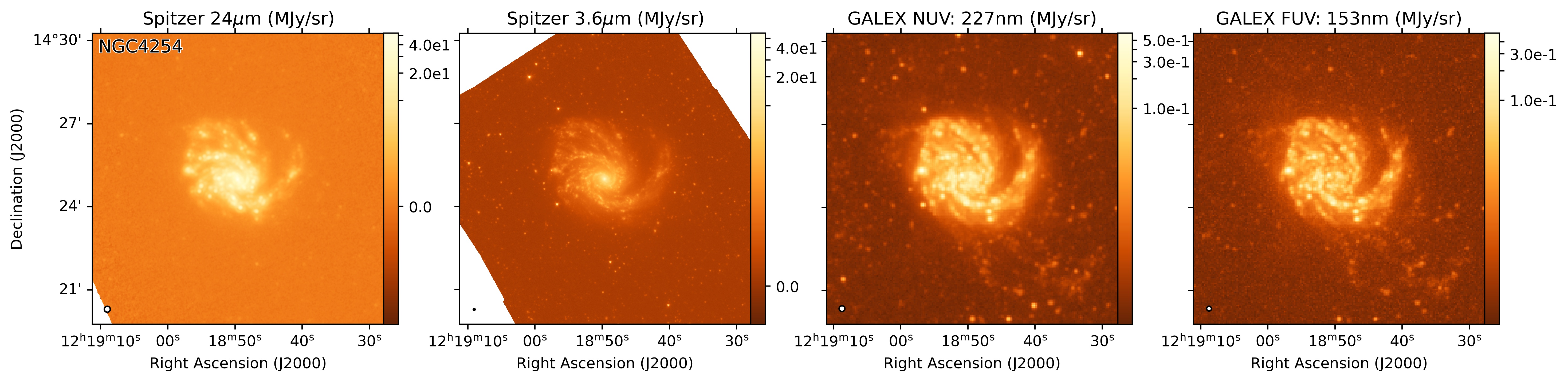
Figure 32: Multiwavelength observations of NGC4254, taken from the Dustpedia database (Clark et al., 2018). Panels as in Figure 30.

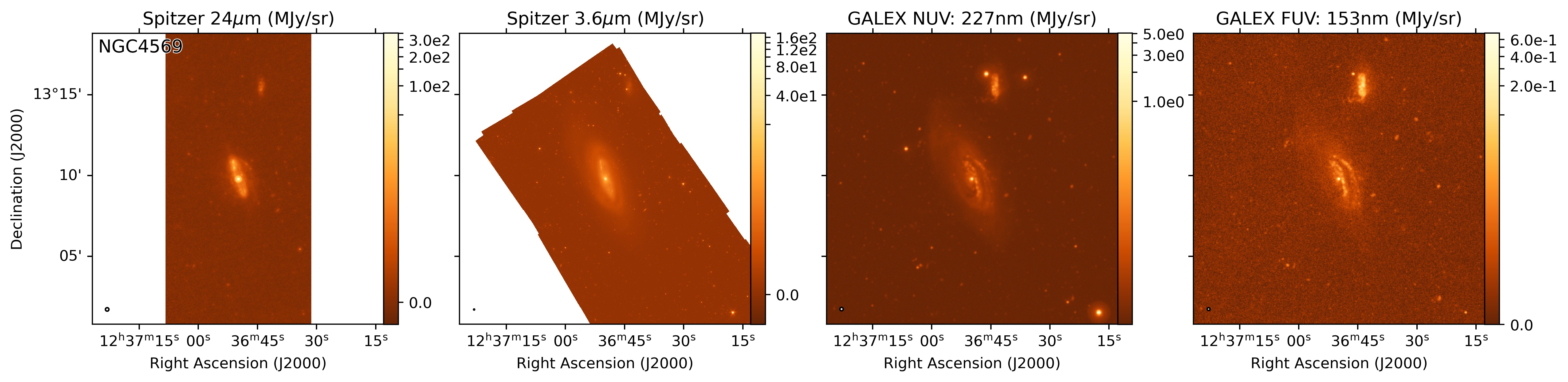
Figure 33: Multiwavelength observations of NGC4569, taken from the Dustpedia database (Clark et al., 2018). Panels as in Figure 30.

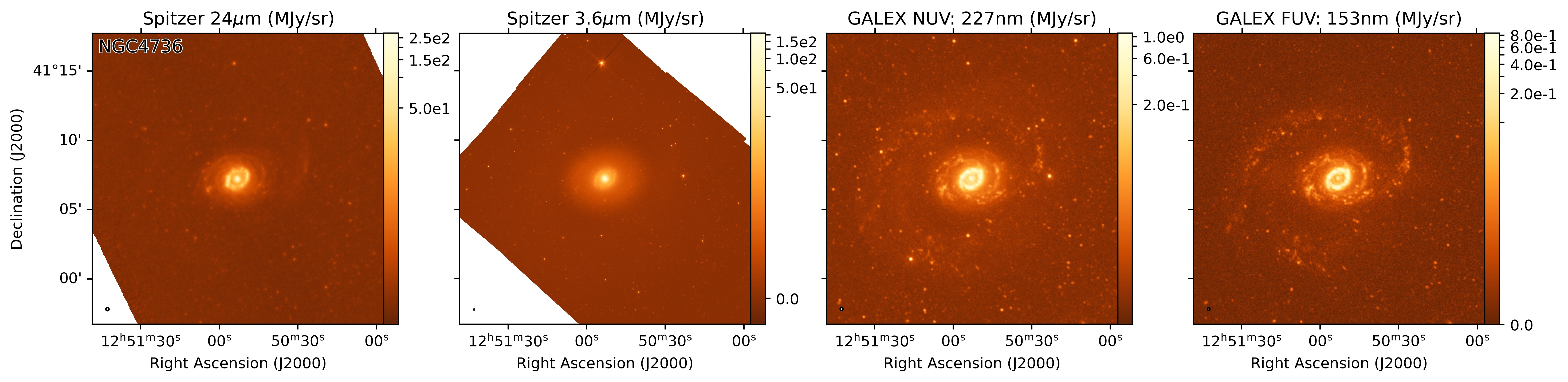
Figure 34: Multiwavelength observations of NGC4569, taken from the Dustpedia database (Clark et al., 2018). Panels as in Figure 30.

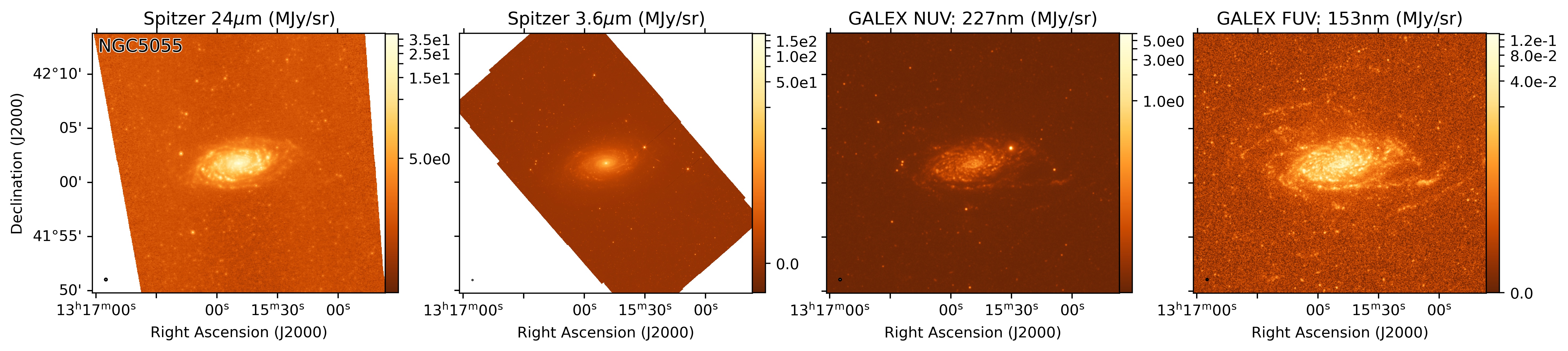
Figure 35: Multiwavelength observations of NGC5055, taken from the Dustpedia database (Clark et al., 2018). Panels as in Figure 30.

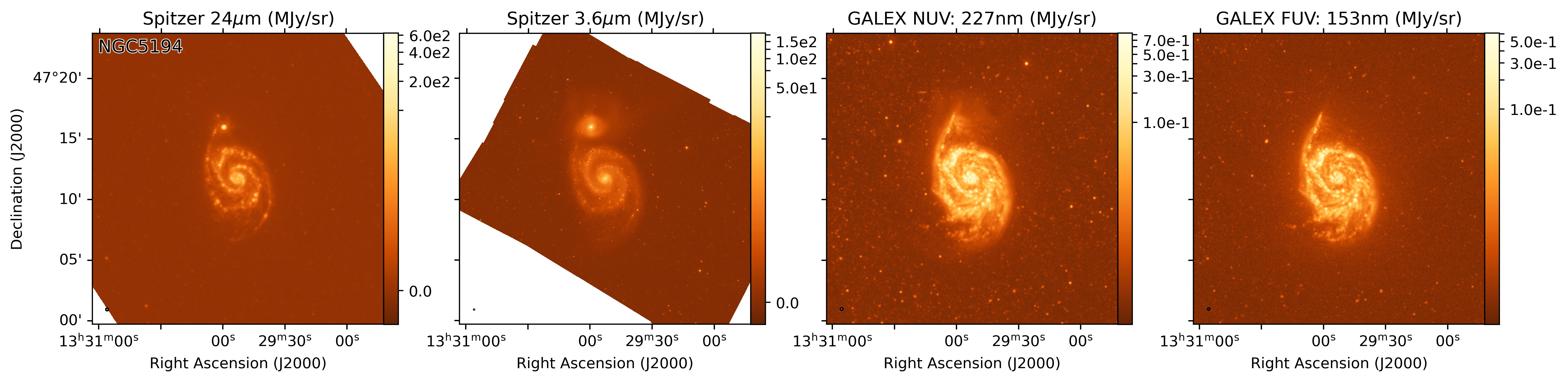
Figure 36: Multiwavelength observations of NGC5194, taken from the Dustpedia database (Clark et al., 2018). Panels as in Figure 30.

We here briefly introduce the 8 galaxies which we consider in this paper. The coordinates, classifications, inclinations, distances and metallicities of the galaxies are listed in Table 1. The listed metallicities are taken from De Vis et al. (2019). All of the galaxies in our sample for which De Vis et al. (2019) list metallicities have slightly sub-solar values of $12+\log({\rm O/H})$, with the largest deficit being $-0.136^{+0.070}_{-0.071}$ in NGC 4254 (compared to the solar value of $12+\log({\rm O/H})=8.69\pm 0.05$; Asplund et al. 2009), equivalent to $Z/Z_{\odot}=0.72^{+0.14}_{-0.10}$. The SCUBA-2 850$\,\mu$m observations of the galaxies in our sample are shown in Figures 1–8, while observations made in the mid-infrared regime with Spitzer and in the ultraviolet regime with GALEX are shown in Figures 29–36 in Appendix C.

3.1 NGC 3034

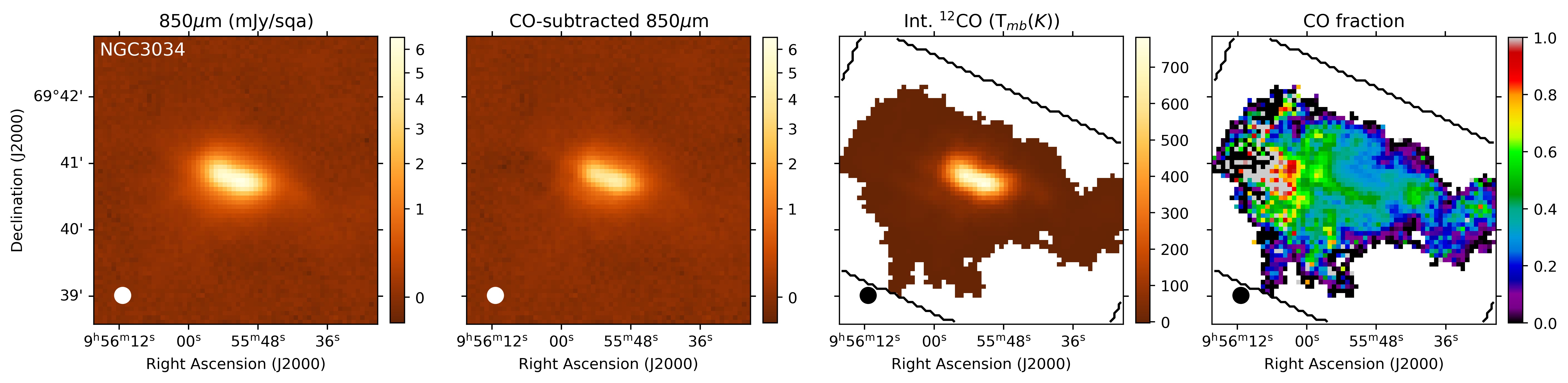
Figure 1: JCMT NGLS observations of NGC 3034. Far left: SCUBA-2 850 $\mu$m data. Centre left: SCUBA-2 850 $\mu$m data, with ¹²CO $J=3\to 2$ contribution subtracted. Both SCUBA-2 images are shown with square-root scaling, in units of mJy arcsec^-2. Centre right: integrated HARP ¹²CO $J=3\to 2$ emission, in main-beam temperature units. Far right: fraction of SCUBA-2 emission in far-left panel that arises from ¹²CO $J=3\to 2$ emission. In the right-hand panels, the footprint of the HARP ¹²CO observation is outlined in black.

NGC 3034 (Messier 82), shown in Figure 1, is a highly-inclined galaxy which is interacting with the neighbouring more massive spiral galaxy M81. At a distance of 3.61 Mpc (Jacobs et al., 2009), M82 is the nearest starburst galaxy to the Milky Way, and has a well-studied ‘superwind’ emanating from the central starburst (e.g. Devine & Bally, 1999). M82, although sometimes classed as irregular, has weak bar and spiral arm features (Mayya et al., 2005), the magnetic field in which has recently been mapped using the POL-2 polarimeter on SCUBA-2 (Pattle et al., 2021), and was previously mapped with SCUPOL (Greaves et al., 2000). HARP ¹²CO $J=3\to 2$ observations of NGC 3034 were presented by Wilson et al. (2012).

Unlike the other galaxies in our sample, M82 is saturated in the Spitzer 24$\mu$m band, and so a star formation rate surface density map cannot be made for it. We nonetheless include it in our sample as it provides a useful point of comparison against previous observations. M82 was observed with the SCUBA camera, the predecessor to SCUBA-2, by Leeuw & Robson (2009). They measured a peak flux density of 1.4 Jy beam^-1, consistent with the peak flux density of 1.5 Jy/beam which we measure before CO subtraction with SCUBA-2. The SCUBA camera’s 850 $\mu$m filter was subject to the same CO contamination effects as is that of SCUBA-2 (e.g. Meijerink et al., 2005).

3.2 NGC 3351

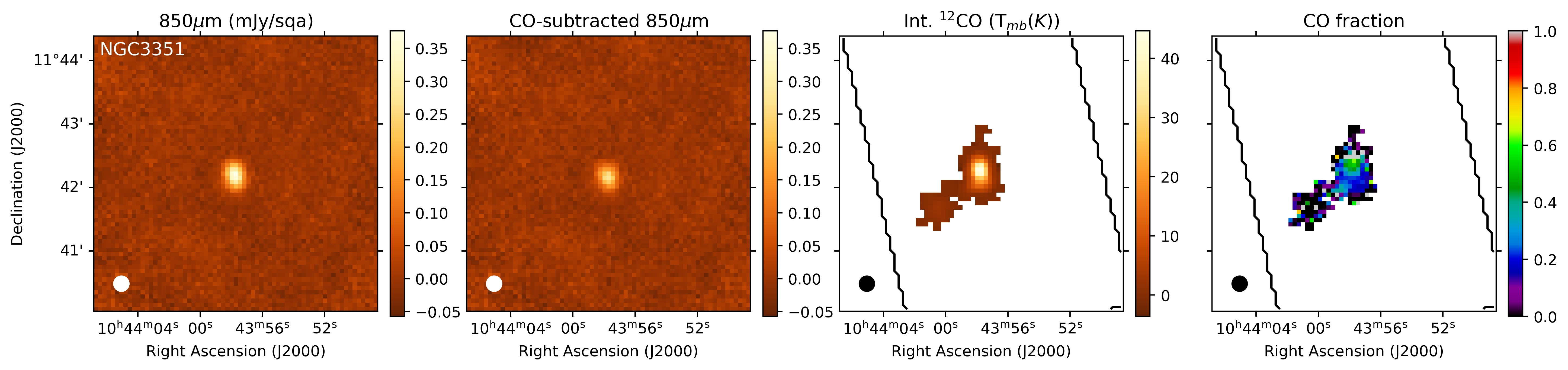
Figure 2: JCMT NGLS observations of NGC 3351. Far left: SCUBA-2 850 $\mu$m data. Centre left: SCUBA-2 850 $\mu$m data, with ¹²CO $J=3\to 2$ contribution subtracted. Both SCUBA-2 images are shown with linear scaling, in units of mJy arcsec^-2. Right-hand panels as in Figure 1.

NGC3351, shown in Figure 2, is a barred spiral galaxy that displays a very young starburst population within a $15\aas@@fstack{\prime\prime}3\times 11\aas@@fstack{\prime\prime}2$ circumnuclear ring (Alloin & Nieto, 1982). We detect but do not resolve the circumnuclear ring in our observations, but do not recover the extended structure of the galaxy. HARP ¹²CO $J=3\to 2$ observations of NGC 3351 were presented by (Wilson et al., 2012) and Tan et al. (2013).

3.3 NGC 3521

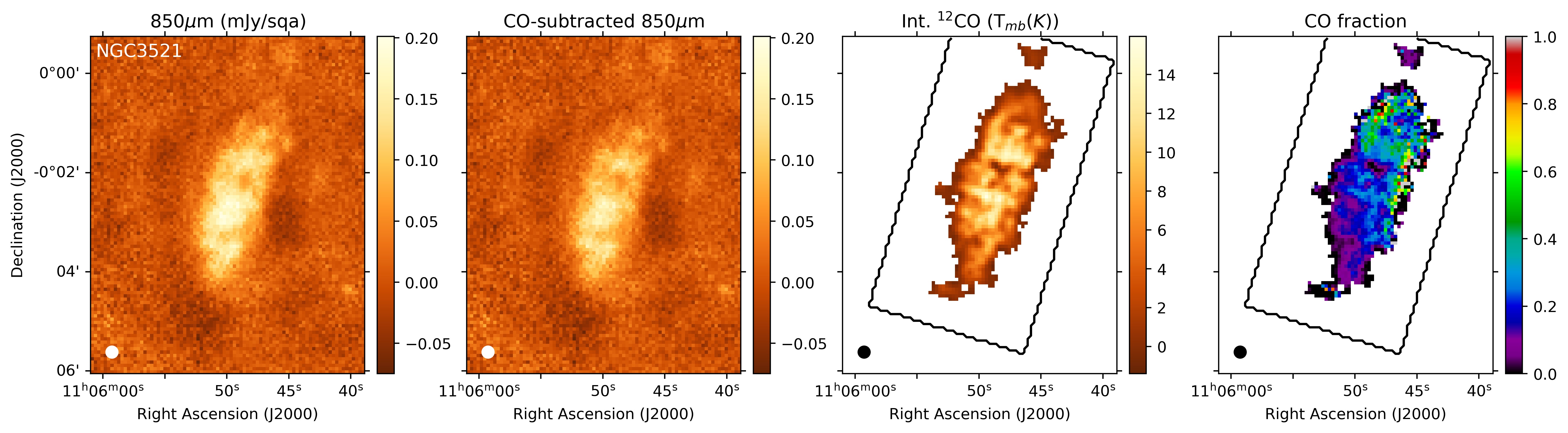
Figure 3: JCMT NGLS observations of NGC 3521. Panels as in Figure 2.

NGC 3521, shown in Figure 3 is a flocculent, weakly-barred spiral galaxy with a tightly-wound two-arm pattern (Liu et al., 2011). NGC 3521 is considered comparable to NGC 5194 (discussed below), as both are metal-rich and quiescently star-forming (Liu et al., 2011). We recover a significant amount of the extended structure of NGC 3521, although the spiral arms are not clearly visible in Figure 3. HARP ¹²CO $J=3\to 2$ observations of NGC 3521 were presented by (Wilson et al., 2012).

3.4 NGC 4254

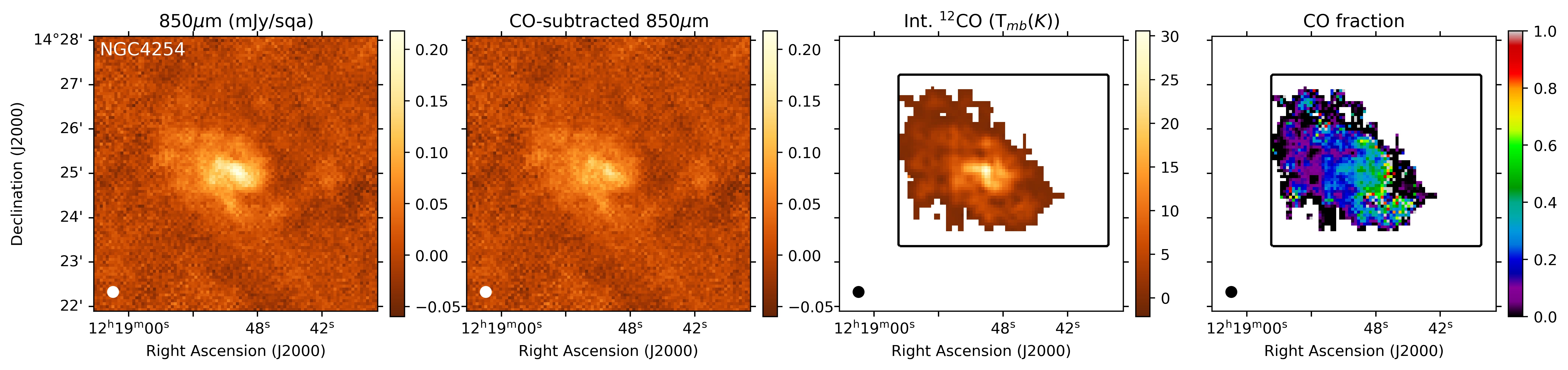
Figure 4: JCMT NGLS observations of NGC 4254. Panels as in Figure 2.

NGC 4254 (Messier 99), shown in Figure 4, is an unbarred Virgo Cluster galaxy with a strong asymmetric spiral pattern which is clearly visible in our SCUBA-2 observations. NGC 4254 has a high star formation rate, particularly in its southern arm, and a tidal tail extending $\sim 250$ kpc northward from the galaxy (not visible in our observations), suggesting that the galaxy is interacting with the centre of the Virgo Cluster (Haynes et al., 2007). HARP ¹²CO $J=3\to 2$ observations of NGC 4254 were presented by Wilson et al. (2009) and Wilson et al. (2012).

3.5 NGC 4569

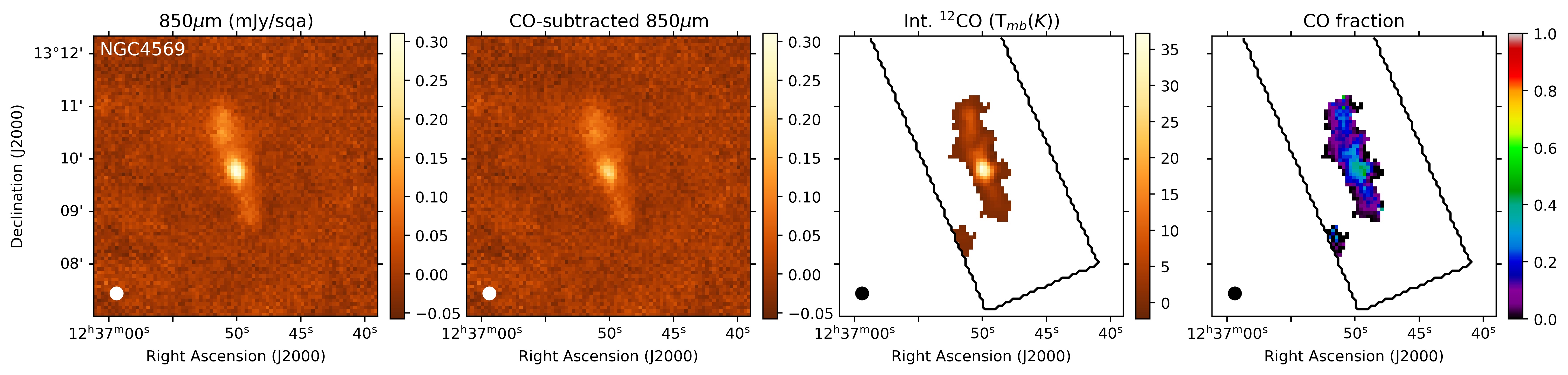
Figure 5: JCMT NGLS observations of NGC 4569. Panels as in Figure 2.

NGC 4569 (Messier 90), shown in Figure 5, is a weakly barred Virgo cluster galaxy which underwent a ram pressure stripping event $\sim 300$ Myr ago, possibly due to motion relative to the intra-cluster medium (Vollmer et al., 2004). The galaxy has a nuclear outflow and a stripped tail (Boselli et al., 2016), which is not visible in the SCUBA-2 data. HARP ¹²CO $J=3\to 2$ observations of NGC 4569 were presented by Wilson et al. (2009) and Wilson et al. (2012).

3.6 NGC 4736

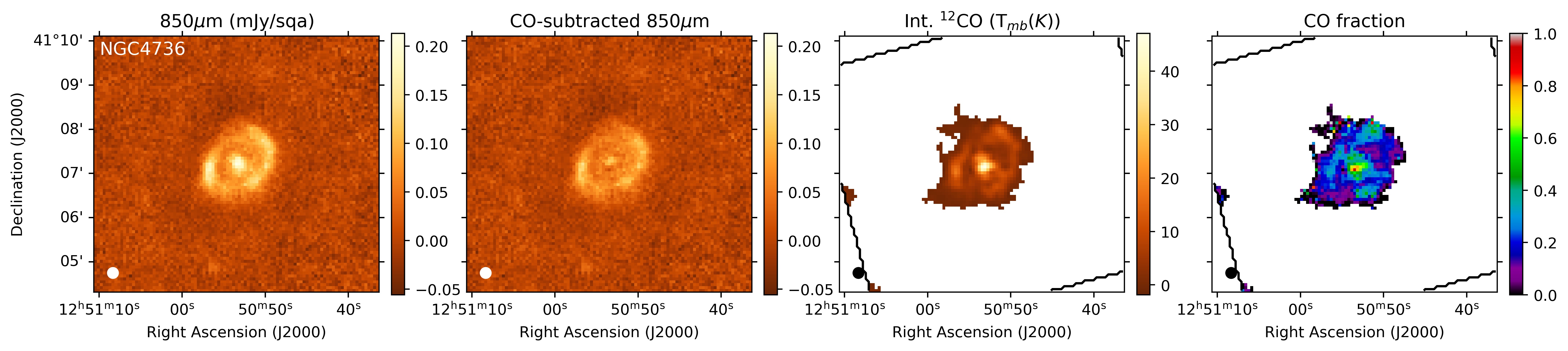
Figure 6: JCMT NGLS observations of NGC 4736. Panels as in Figure 2.

NGC 4736 (Messier 94), shown in Figure 6, is an actively star-forming unbarred ring galaxy. The galaxy has a weak and diffuse outer ring, which is at best marginally detected in our SCUBA-2 observations, and a bright and actively star-forming inner pseudo-ring (Wong & Blitz, 2000; Waller et al., 2001). This inner pseudo-ring, with a radius of $\sim 47^{\prime\prime}$ (Chyży & Buta, 2008), is clearly visible in our SCUBA-2 data. HARP ¹²CO $J=3\to 2$ observations of NGC 4736 were presented by (Wilson et al., 2012).

3.7 NGC 5055

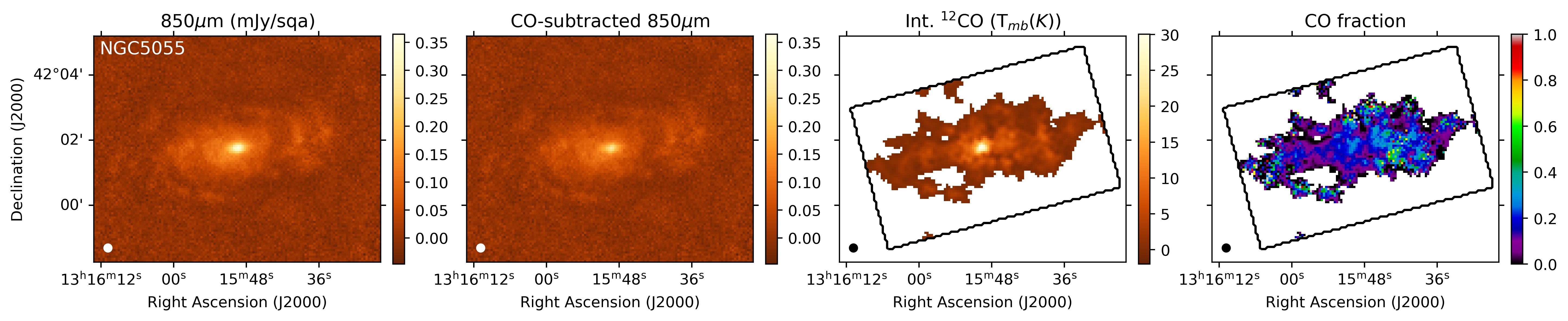
Figure 7: JCMT NGLS observations of NGC 5055. Panels as in Figure 2.

NGC 5055 (Messier 63), shown in Figure 7, is a moderately inclined unbarred spiral galaxy with a very large, warped Hi disc (Battaglia et al., 2006), in which massive stars have recently formed (Thilker et al., 2007). The spiral structure of the galaxy is clearly visible in our SCUBA-2 observations. HARP ¹²CO $J=3\to 2$ observations of NGC 5055 were presented by (Wilson et al., 2012).

3.8 NGC 5194

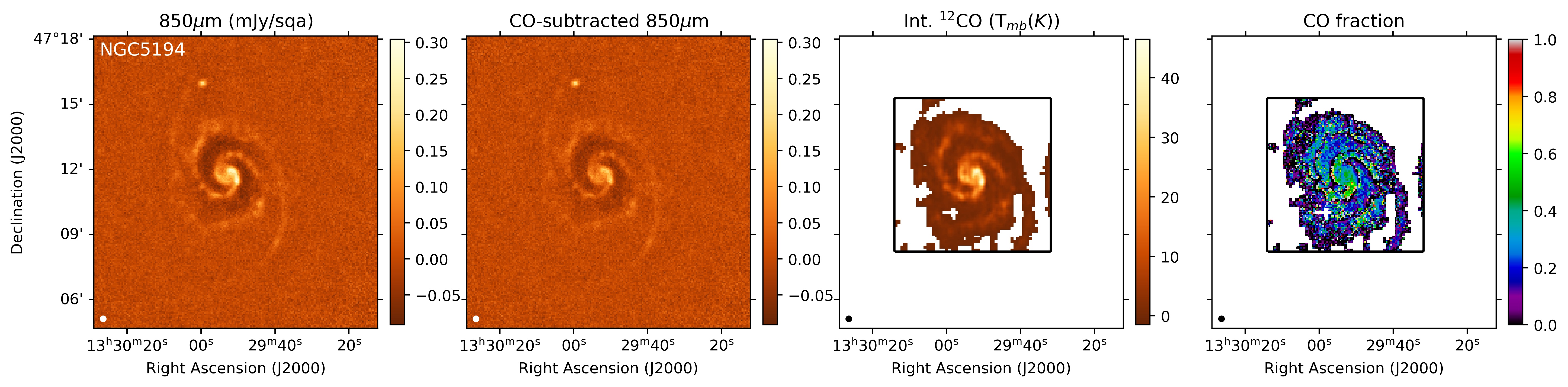
Figure 8: JCMT NGLS observations of NGC 5194. Panels as in Figure 2.

NGC 5194 (Messier 51a) is a face-on two-arm grand-design spiral galaxy, interacting with its neighbour, M51b. Both are shown in Figure 8. Star formation in NGC 5194 is mostly taking place in the galactic centre and spiral arms (Schinnerer et al., 2017). CO observations of NGC 5194 show chains of GMCs emerging from the spiral arms into the interarm regions (Koda et al., 2009; Schinnerer et al., 2017), but these features are not resolved in our observations. HARP ¹²CO $J=3\to 2$ observations of NGC 3521 were presented by (Wilson et al., 2012) and Vlahakis et al. (2013).

Unlike the other galaxies in our sample, NGC 5194 was observed using the PONG 900 observing mode (Holland et al., 2013). In order to be as consistent as possible, we have applied the same data reduction parameters to all of the galaxies in our sample. However, the data reduction process which we describe in Section 2 does not appear to be optimal for NGC 5194; the SCUBA-2 images in Figure 8 show significant negative bowling in the inter-arm regions. This suggests that recoverable large-scale emission from NGC 5194 has been lost in the data reduction process, and affects our estimates of total flux density for the galaxy listed in Table 3.

NGC 5194 was previously observed with SCUBA (Meijerink et al., 2005). These authors found an exponential disc in their 850$\mu$m observations, which we do not recover here. They measured a peak flux density $\gtrsim 117$ mJy beam^-1, including a contribution from CO. We measure a peak flux density of 69 mJy beam^-1 before CO subtraction, again suggesting that the data reduction strategy which we employ in this work is not optimal for these observations of NGC 5194. Interestingly, after subtraction of their modelled exponential disc, Meijerink et al. (2005) find a peak flux density of $\gtrsim 72$ mJy beam^-1, consistent with the peak flux density which we measure. This suggests that we may be recovering the emission from more compact structures in NGC 5194 quite well.

4 Comparison with molecular and atomic gas

We investigated the correlation between SCUBA-2 850$\mu$m flux density and atomic and molecular gas column density.

We measured Hi column density ($N({\rm H}\textsc{i})$) using Very Large Array (VLA) Hi observations, taken from the THINGS (Walter et al., 2008) (NGC 3351, 3521, 4736, 5055, 5194) and VIVA (Chung et al., 2009) (NGC 4254, 4569) surveys, and from de Blok et al. (2008) for NGC 3034. The VLA data were converted from Jy beam^-1 to brightness temperature ($T_{B}$) using the relation

$$T_{B}=I_{{\rm H}\textsc{i}}\times\frac{6.07\times 10^{5}}{\theta_{maj}\theta_{min}}\,{\rm K}\,({\rm Jy\,beam}^{-1})^{-1}$$ (2)

(cf. Walter et al., 2008), where $I_{{\rm H}\textsc{i}}$ is Hi brightness and $\theta_{maj}$ and $\theta_{min}$ are the major and minor beam widths, respectively. $N({\rm H}\textsc{i})$ was then calculated using the relation

$$N({\rm H}\textsc{i})=1.823\times 10^{18}\,{\rm cm}^{-2}\,{\rm K}^{-1}\times T_{B}$$ (3)

(cf. Walter et al., 2008).

We measured H₂ column density ($N({\rm H}_{2})$) using the Nobeyama ¹²CO 1$\to$0 observations from the COMING (Sorai et al., 2019) and CO ATLAS (Kuno et al., 2007) surveys which we used to define the data reduction masks as described in Section 2. $N({\rm H}_{2})$ was calculated using the relation

$$N({\rm H}_{2})=X_{\rm CO}\int T_{mb}{\rm}d\nu,$$ (4)

taking the integrated main-beam temperature maps from the COMING and CO-ATLAS databases, and using a CO X-factor of $X_{\rm CO}=2\times 10^{20}$ cm^-2 (K km s^-1)^-1 (Bolatto et al., 2013). Bolatto et al. (2013) give an uncertainty on $X_{\rm CO}$ of $\pm 30$% in the Milky Way disc, and $X_{\rm CO}$ is expected to vary further with metallicity. We assume a constant $X_{\rm CO}$ in order to directly compare between ¹²CO and SCUBA-2 850$\mu$m emission as molecular gas tracers for the galaxies in our sample, but note that this assumption introduces an additional uncertainty on the values of $N({\rm H}_{2})$ determined from ¹²CO observations.

The Nobeyama 45m ¹²CO data have a resolution of 17^′′ (Sorai et al., 2019). The VLA data have a variety of resolutions. Where the VLA resolution was $<17^{\prime\prime}$ we smoothed both the SCUBA-2 and the $N({\rm H}\textsc{i})$ maps to 17^′′. Where the VLA resolution was $>17^{\prime\prime}$ (NGC 3034 and NGC 4254), we smoothed the SCUBA-2 and $N({\rm H}_{2})$ maps to the geometric mean of the VLA beam’s major and minor axes, 34.3^′′ and 29.4^′′ for NGC 3034 and NGC 4254 respectively.

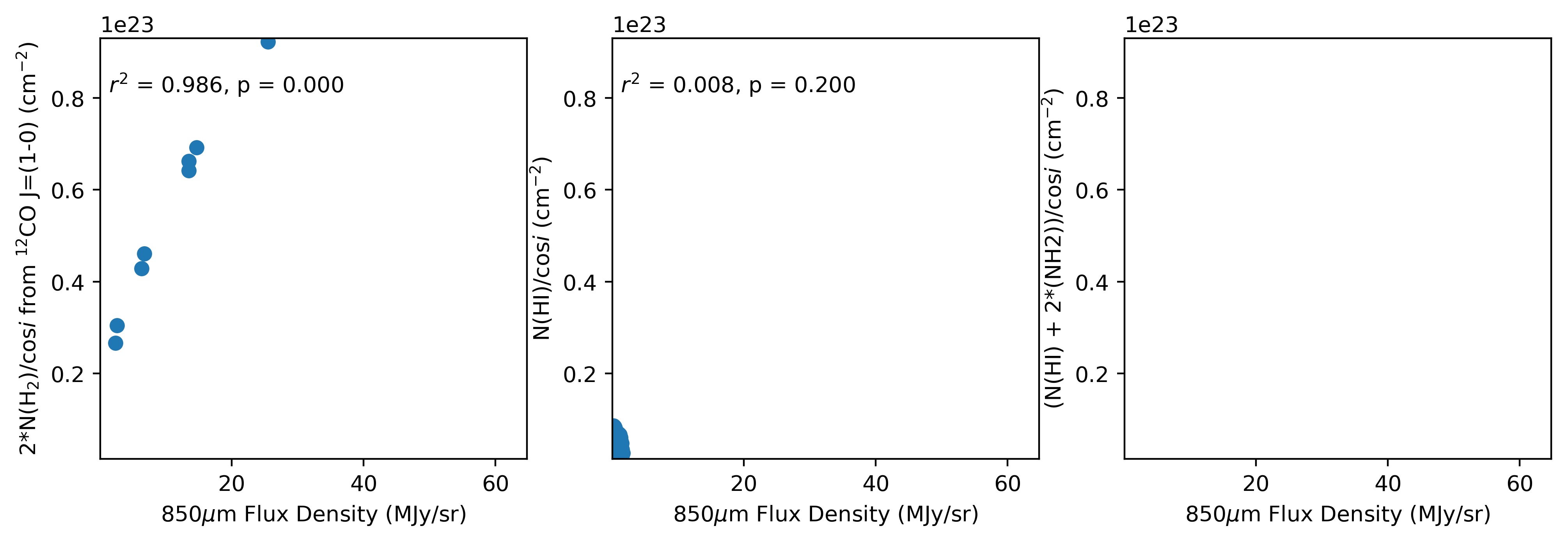
Figure 13: Comparison of dust and gas emission in NGC 3034. Left: SCUBA-2 850$\mu$m surface brightness compared to column density of molecular gas derived from Nobeyama 45m ${12}$CO $J=1\to 0$ measurements. Centre: 850$\mu$m surface brightness compared to column density of atomic gas derived from VLA Hi measurements. Right: SCUBA-2 850$\mu$m surface brightness compared to total gas column density. Note that the VLA Hi observations of NGC3034 are saturated towards the centre of the galaxy, resulting in there being no overlap between the two gas density tracers.

We corrected the derived column density for inclination angle using the inclination values given in the Dustpedia database (Clark et al., 2018) and listed in Table 3. Comparisons between SCUBA-2 850$\mu$m flux density and $N({\rm H\textsc{i}})$, $N({\rm H_{2}})$ and total hydrogen column density ($N({\rm H\textsc{i}})+2N({\rm H_{2}})$) are shown in Figure 13–20 in Appendix A.

¹²CO emission and 850$\mu$m flux density are consistently correlated with one another, suggesting that both are tracing similar material, i.e. molecular gas (e.g. Bolatto et al. 2013). We typically see no strong correlation between Hi and 850$\mu$m, with the possible exceptions of NGC 4569 and 4736. Generally, the less well-resolved sources show a stronger correlation between Hi and 850$\mu$m dust emission. This further suggests that the 850$\mu$m dust emission detected by SCUBA-2 is preferentially tracing the molecular gas, as Hi and 850$\mu$m dust emission are better-correlated where Hi and ¹²CO emission occupy the same beam. We note that in NGC 3034 the VLA data are saturated at high column densities, so there is no overlap between the ¹²CO and Hi measurements.

In the following section, we measure column density of $N({\rm H}_{2})$ from dust emission, taking the dust emission to trace the molecular gas. However, to do so, we must assume a gas-to-dust ratio, as discussed below. The gas-to-dust ratio depends on metallicity and varies somewhat between the galaxies in our sample (De Vis et al. 2019; cf. Table 1). As discussed above, we expect $X_{\rm CO}$ to vary systematically within and between galaxies in our sample. We are not able to distinguish between variation in gas-to-dust ratio and in $X_{\rm CO}$, and so do not attempt to use the ratio between ¹²CO emission and 850$\mu$m flux density to determine gas-to-dust ratios for the galaxies which we consider. We comment on the consequences of using a constant gas-to-dust ratio further below.

5 SED fitting

We measured dust column densities, temperatures and opacity indices for the galaxies in our sample by fitting their spectral energy distributions (SEDs) using SCUBA-2 850$\mu$m and Herschel Space Observatory data. We took Herschel 70$\mu$m, 100$\mu$m (where present), 160$\mu$m, 250$\mu$m and 350$\mu$m data from the Dustpedia database (Clark et al., 2018). We excluded the Herschel 500$\mu$m data as being too low-resolution (36.6^′′; Griffin et al. 2010), and, being away from the SED peak but shorter-wavelength than the SCUBA-2 850$\mu$m data, not necessary in order to produce a well-constrained fit. The lowest-resolution data set which we use is Herschel 350$\mu$m, with a resolution of 25.2^′′ (Griffin et al., 2010).

5.1 Spatial filtering

SCUBA-2 is restricted in the spatial scales to which it is sensitive due to the need to distinguish between astrophysical and atmospheric signal (e.g. Chapin et al., 2013). SCUBA-2 is fundamentally insensitive to signal on scales larger than its array size (600^′′), but in practice the maximum size scale recovered is set by a combination of the mask used and the maximum size scale set in the reduction process, as discussed in Section 2. Herschel images, having been taken above the atmosphere, are not subject to such constraints. It is therefore necessary to match the spatial scales in the Herschel and SCUBA-2 observations before comparing the data sets.

We removed the large-scale structure from the Herschel observations by passing them through the SCUBA-2 pipeline in the manner described by Sadavoy et al. (2013). Similarly to the method for CO subtraction, the Herschel data are added to the SCUBA-2 bolometer time series, and the reduction process is repeated, including the application of the mask. In this case the Herschel data are scaled to be a small positive perturbation on the SCUBA-2 signal in order to minimise the effect of the Herschel data on map convergence. The SCUBA-2 map is then subtracted from the Herschel+SCUBA-2 map and the scaling applied to the Herschel data is reversed, leaving the spatially-filtered Herschel signal.

5.2 SED fitting

We used the $Starlink$ Kappa package (Currie et al., 2014) to convolve the 850$\mu$m data and all of the filtered Herschel maps to 350$\mu$m resolution (25.2^′′), and to grid all of the maps to 16^′′ pixels. We then fitted SEDs pixel-by-pixel using the relation

$$F_{\nu}=\Sigma_{\rm dust}B_{\nu}(T)\kappa_{0}\left(\frac{\nu}{\nu_{0}}\right)^{\beta}$$ (5)

(cf. Hildebrand, 1983), where $\Sigma_{\rm dust}$ is surface density of dust in units of g cm^-2, $B_{\nu}(T)$ is the Planck function at temperature $T$, dust opacity $\kappa_{0}=1.92$ cm² g^-1 at a reference frequency $\nu_{0}=0.857\,$THz (350$\mu$m) (Draine, 2003), and $\beta$ is dust opacity index.

We restricted our fitting to pixels where all the flux density values have an SNR greater than 3. We first fitted with $\Sigma_{\rm dust}$, $T$ and $\beta$ as free parameters. We then repeated the fitting process, with $\beta$ fixed at its median value from the previous fit. In both cases, we rejected any pixels where the fitted values of any of $\Sigma_{\rm dust}$, $T$ or $\beta$ have uncertainties of $>50\%$. This criterion only excluded a significant number of pixels in the $\beta$-free fit for NGC 3034.

We converted $\Sigma_{\rm dust}$ to molecular hydrogen column density ($N({\rm H}_{2})$) using the relation

$$N({\rm H}_{2})=100\times\frac{\Sigma_{\rm dust}}{\mu m_{\textsc{h}}},$$ (6)

where mean molecular mass is taken to be $\mu=2.8$, $m_{\textsc{h}}$ is the mass of hydrogen and the gas-to-dust ratio is taken to be 100. We note that the galaxies in our sample have metallicities similar to, but slightly less than, the solar value (cf. Table 1), and so these values of $N({\rm H}_{2})$ may be slightly underestimated. Moreover, the value of the dust-to-gas ratio may vary significantly within galaxies (e.g. Williams et al. 2018), creating a further systematic uncertainty on $N({\rm H}_{2})$. The values of $N({\rm H}_{2})$ determined using this equation are not yet corrected for the effect of inclination angle.

We show maps of best-fit $N({\rm H}_{2})$, $T$, $\beta$, their uncertainties and reduced $\chi^{2}$ values for each galaxy in Appendix B. The mean, median maximum and minimum values for each of the fitted parameters are listed in Table 6 for the $\beta$-free case, and in Table 7 for the median-$\beta$ case. $N({\rm H}_{2})$ values are at this stage shown without correction for inclination angle in order to show the fitted values. The median value of $\beta$ varies in the range $1.63-2.26$. The mean and median values of the fitted parameters are similar, except in the case of $\Sigma_{dust}$ for NGC 3034 and, to a lesser extent, NGC 5194, where the mean value is significantly higher than the median. This is due to the large dynamic range in the NGC 3034 and NGC 5194 observations. The values of $\Sigma_{dust}$ and $T$ are similar in the $\beta$-free and median-$\beta$ cases, suggesting that the variation in $\beta$ within the galaxies is not very large.

5.3 SCUBA-2 flux loss

We compared the total flux density in the Herschel 250$\mu$m maps before and after they were passed through the SCUBA-2 pipeline in order to assess the likely amount of large-scale structure lost in the SCUBA-2 data reduction process. The 250$\mu$m data were chosen as having the resolution most similar to the SCUBA-2 850$\mu$m data: 18.1^′′ (Griffin et al., 2010) compared to 14.1^′′ for SCUBA-2. The total flux densities before and after filtering are listed in Table 4. The mean fraction of flux lost in the filtering process is $0.58\pm 0.15$, and the median is 0.59. However, this flux is not lost evenly across the map, with small-scale structures being recovered well, and extended, diffuse emission being lost. The best-recovered galaxy is the bright and relatively compact NGC 3034, where only 32% of the Herschel 250$\mu$m flux is lost. The worst-recovered is NGC 3351, only the central region of which is visible in the SCUBA-2 image (see Figure 2). In this case, 85% of the Herschel flux density – mostly associated with the galactic disc – is lost. Despite this, the compact and strongly-peaked central region is recovered quite well.

Galaxy	250$\mu$m Flux Density		Fraction lost
	Original	Filtered
	(Jy)
NGC 3034	451.0	305.8	0.32
NGC 3351	27.0	5.5	0.85
NGC 3521	104.1	58.3	0.56
NGC 4254	69.1	27.3	0.56
NGC 4569	41.0	13.6	0.47
NGC 4736	59.1	22.5	0.65
NGC 5055	134.4	52.3	0.63
NGC 5194	183.5	82.2	0.61

Table 4: Comparison of Herschel 250$\mu$m flux densities before and after filtering.

	SED,$\beta$-free	SED,median-$\beta$	250,$\beta$-free	250,median-$\beta$
$N({\rm H}_{2})$	Free parameter in SED fit	Free parameter in SED fit	From SPIRE $F_{\nu}(250\mu{\rm m})$	From SPIRE $F_{\nu}(250\mu{\rm m})$
$T$	Free parameter in SED fit	Free parameter in SED fit	From $\beta$-free SED fit	From $\beta$-median SED fit
$\beta$	Free parameter in SED fit	Fixed at median value from $\beta$-free fit	From $\beta$-free SED fit	Fixed at median value from $\beta$-free fit
Filtered?	Yes	Yes	No	No

Table 5: A summary of our four measures of $N({\rm H}_{2})$.

We note again that we have optimised the SCUBA-2 DR process for image fidelity, rather than for large-scale structure recovery, as described in Section 2. An alternative data reduction scheme might be able to recover a larger fraction of the large-scale emission. However, these results show that SCUBA-2 will inherently be insensitive to a significant fraction of the submillimetre flux density from well-resolved galaxies such as those in our sample.

In subsequent analysis, in order to evaluate the effects of the SCUBA-2 flux loss, we use measures of $\Sigma_{dust}$ and $N({\rm H}_{2})$ determined in two ways: (1) from SED fitting, and therefore subject to flux loss due to atmospheric filtering; and (2) from Herschel SPIRE 250$\mu$m flux density using equation 5, using the $T$ and $\beta$ values from SED fitting, and therefore calculated from the full column of emission. These measures of $\Sigma_{dust}$ and $N({\rm H}_{2})$ are summarised in Table 5 and discussed further below.

	$\beta$ free
	$\Sigma_{dust}$ ($\times 10^{-5}$ g cm-2)				Temperature (K)				Dust Opacity Index $\beta$
Galaxy	Mean	Median	Min	Max	Mean	Median	Min	Max	Mean	Median	Min	Max
NGC 3034	$38.0\pm 72.9$	$10.4\pm 5.4$	1.5	304	$30.5\pm 4.4$	$30.7\pm 2.8$	21.6	38.9	$2.05\pm 0.45$	$2.03\pm 0.30$	1.24	3.13
NGC 3351	$12.7\pm 3.4$	$12.4\pm 2.7$	8.4	17.6	$27.8\pm 0.9$	$27.6\pm 0.6$	26.6	29.1	$2.01\pm 0.17$	$2.03\pm 0.15$	1.78	2.19
NGC 3521	$10.9\pm 4.9$	$10.4\pm 3.6$	2.3	21.2	$25.5\pm 1.9$	$25.2\pm 1.3$	22.0	29.3	$1.81\pm 0.39$	$1.86\pm 0.32$	1.07	2.43
NGC 4254	$6.2\pm 4.9$	$4.2\pm 2.4$	1.1	20.9	$25.1\pm 2.5$	$25.1\pm 1.9$	19.7	32.0	$2.02\pm 0.40$	$1.98\pm 0.30$	1.17	3.21
NGC 4569	$7.8\pm 3.3$	$8.0\pm 2.5$	2.4	13.6	$24.2\pm 2.5$	$24.0\pm 1.8$	19.4	28.8	$1.84\pm 0.30$	$1.75\pm 0.12$	1.46	2.79
NGC 4736	$4.7\pm 1.8$	$4.8\pm 1.3$	1.1	9.1	$32.2\pm 2.6$	$32.8\pm 1.5$	23.8	36.3	$1.69\pm 0.23$	$1.63\pm 0.09$	1.37	2.69
NGC 5055	$6.5\pm 5.6$	$4.7\pm 2.2$	1.1	33.8	$23.4\pm 2.4$	$23.7\pm 1.3$	14.9	27.4	$1.98\pm 0.56$	$1.86\pm 0.28$	1.09	4.69
NGC 5194	$9.1\pm 10.5$	$4.2\pm 2.3$	0.78	43.3	$23.1\pm 2.4$	$23.3\pm 1.7$	17.5	29.4	$2.32\pm 0.56$	$2.26\pm 0.32$	1.20	3.74

Table 6: A summary of the SED fitting results for the galaxies in our sample, with $\beta$ as a free parameter.

	Median-$\beta$
	$\Sigma_{dust}$ ($\times 10^{-5}$ g cm-2)				Temperature (K)				$\beta$
Galaxy	Mean	Median	Min	Max	Mean	Median	Min	Max
NGC 3034	$35.7\pm 68.4$	$10.6\pm 6.9$	1.14	293	$30.7\pm 3.3$	$31.2\pm 2.5$	22.8	38.5	2.03
NGC 3351	$12.6\pm 2.4$	$12.7\pm 1.9$	9.1	15.9	$27.6\pm 0.9$	$27.5\pm 0.8$	26.7	28.8	2.03
NGC 3521	$10.5\pm 4.6$	$10.1\pm 3.1$	2.0	20.5	$25.1\pm 1.1$	$25.2\pm 0.9$	22.9	26.9	1.86
NGC 4254	$6.4\pm 4.7$	$4.9\pm 2.8$	1.0	20.4	$25.0\pm 0.7$	$25.0\pm 0.4$	23.8	27.2	1.98
NGC 4569	$7.7\pm 3.4$	$8.5\pm 2.0$	1.7	14.8	$24.6\pm 1.3$	$24.5\pm 0.6$	22.2	27.1	1.75
NGC 4736	$4.5\pm 1.6$	$4.6\pm 1.2$	1.1	7.5	$32.9\pm 3.1$	$32.3\pm 1.1$	27.9	41.4	1.63
NGC 5055	$6.7\pm 5.0$	$5.6\pm 2.3$	1.2	27.9	$23.8\pm 1.3$	$23.9\pm 0.8$	20.3	26.4	1.86
NGC 5194	$6.5\pm 6.7$	$3.9\pm 1.8$	0.83	33.3	$23.5\pm 2.3$	$24.2\pm 1.0$	16.6	28.9	2.26

Table 7: A summary of the SED fitting results for the galaxies in our sample, with $\beta$ fixed at its median value from the free-parameter fit.

6 Star Formation Law

We measured surface density of star formation ($\Sigma_{\textsc{sfr}}$) for the galaxies in our sample, in order to investigate the relationship between $\Sigma_{\textsc{sfr}}$ and $\Sigma_{gas}$ both within and between the galaxies.

6.1 Creating star formation surface density maps

We measured the star formation rate in the galaxies in our sample using the method described by Leroy et al. (2008). We measured unobscured star formation using GALEX far-ultraviolet (FUV) emission ($I_{\textsc{fuv}}$) and obscured star formation using Spitzer Space Telescope 24$\mu$m emission ($I_{24}$). The older stellar population was accounted for using Spitzer 3.6$\mu$m emission ($I_{3.6}$). All of these maps were taken from the Dustpedia database (Clark et al., 2018). NGC 3034 is saturated in the Spitzer 24$\mu$m band, and so is excluded from further analysis. The Spitzer and GALEX observations are shown in Figures 29–36 in Appendix C. We smoothed all of the data sets to $25\aas@@fstack{\prime\prime}2$ to match the resolution of the SED-fitted maps, and again gridded the maps to 16^′′ pixels.

Any pixels with significant GALEX near-ultraviolet (NUV) emission, i.e. where $I_{\textsc{nuv}}/I_{\textsc{fuv}}>15$, were excluded from the analysis, in order to avoid contamination by foreground stars (Leroy et al., 2008). We then estimated the FUV flux density associated with star formation ($I_{\textsc{fuv,sf}}$) using the relation

$$I_{\textsc{fuv,sf}}=I_{\textsc{fuv}}-\alpha_{\textsc{fuv}}I_{3.6},$$ (7)

taking $\alpha_{\textsf{fuv}}=3\times 10^{-3}$, and the 24$\mu$m flux density associated with star formation ($I_{24,\textsc{sf}}$) using the relation

$$I_{24,\textsc{sf}}=I_{24}-\alpha_{24}I_{3.6},$$ (8)

taking $\alpha_{24}=0.1$ (Leroy et al., 2008). We then estimated the surface density of star formation to be

$$\Sigma_{\textsc{sfr}}=8.1\times 10^{-2}I_{\textsc{fuv,sf}}+3.2\times 10^{-3}I_{24,\textsc{sf}}.$$ (9)

By using these values, we have implicitly assumed a Chabrier (2003) Initial Mass Function (IMF) (Leroy et al., 2008).

We assumed calibration uncertainties of 4.5% on GALEX FUV, 5% on Spitzer 24$\mu$m and 3% on Spitzer 3.6$\mu$m measurements, as per Clark et al. (2018). We assumed a 33% uncertainty on the $I_{24,\textsc{sf}}$ term in equation 9, following Leroy et al. (2008) and Ford et al. (2013).

The final $\Sigma_{\textsc{sfr}}$ maps are shown in Appendix D. These maps are expected to trace star formation on timescales $<100$ Myr (Leroy et al., 2008). The mean age of the stellar population contributing to the unobscured star formation rate is $\sim 10$ Myr, while the stellar population contributing to the obscured star formation rate has a mean age of $\sim 5$ Myr (Kennicutt & Evans, 2012). 90% of the stellar population contributing to each measure is expected to have an age $<100$ Myr (Kennicutt & Evans, 2012).

We note that in every case, the surface density of obscured (24$\mu$m-traced) star formation is greater than that of unobscured (FUV-traced) star formation. The mean contributions from obscured and unobscured star formation to $\Sigma_{\textsc{sfr}}$ are shown in Figure 9. This suggests that the star formation being traced may be preferentially occurring on timescales as short as $\sim 5$ Myr (Rieke et al., 2009; Kennicutt & Evans, 2012).

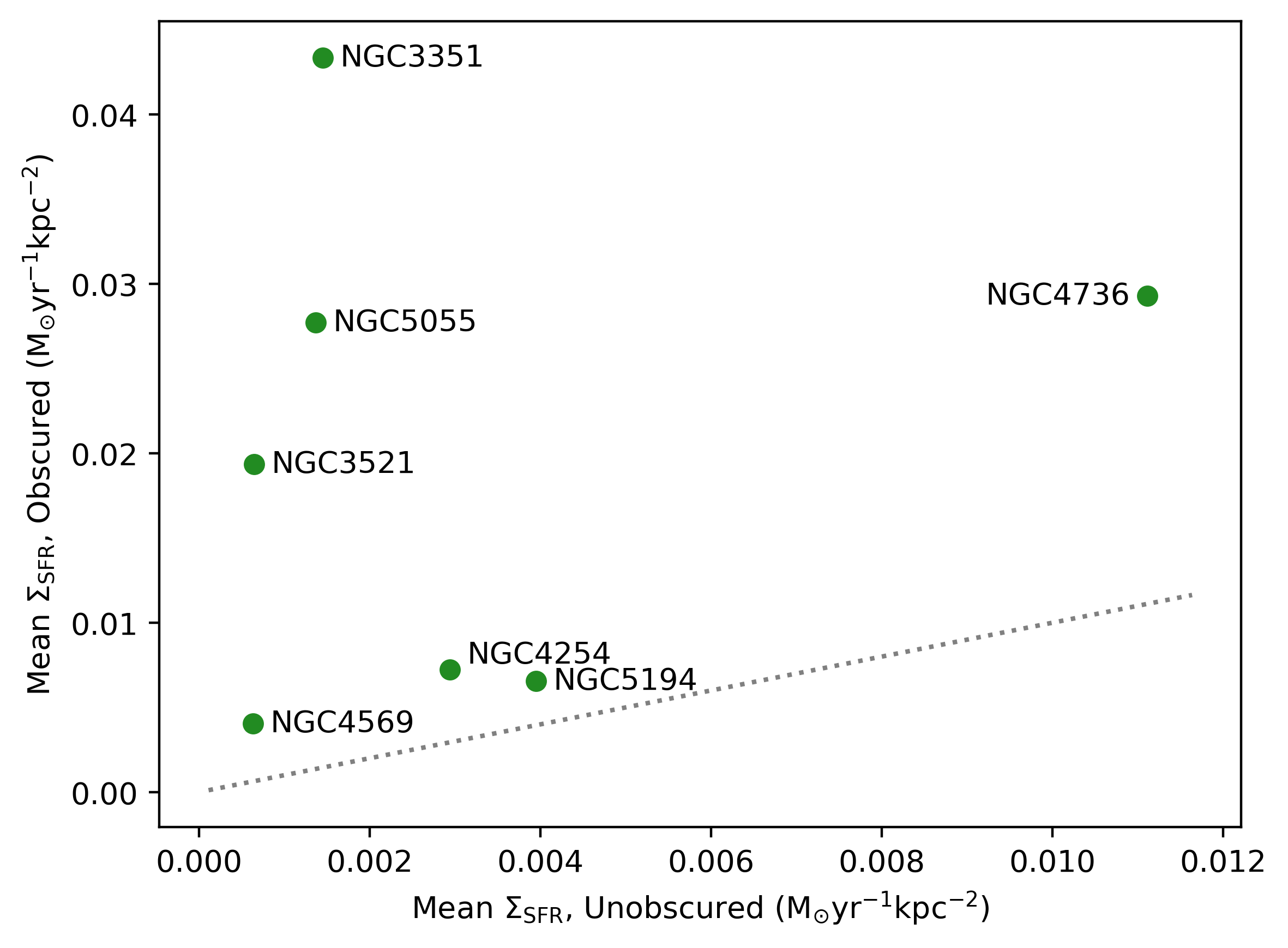
Figure 9: Mean contributions to $\Sigma_{\textsc{sfr}}$ from obscured (24$\mu$m-traced) and unobscured (FUV-traced) star formation for the galaxies in our sample. Dotted grey line marks the 1:1 relationship.

6.2 Resolved Kennicutt-Schmidt Law

	SED-fit						H250
	$\beta$ free			median $\beta$			$\beta$ free			median $\beta$
Galaxy	$N$	$C$	$r^{2}$	$N$	$C$	$r^{2}$	$N$	$C$	$r^{2}$	$N$	$C$	$r^{2}$
NGC 3351	0.60$\pm$0.04	$-$1.84$\pm$0.06	0.991	0.77$\pm$0.19	$-$2.10$\pm$0.30	0.887	0.97$\pm$0.15	$-$2.49$\pm$0.25	0.952	1.49$\pm$0.28	$-$3.35$\pm$0.45	0.935
NGC 3521	0.75$\pm$0.02	$-$2.59$\pm$0.03	0.958	0.71$\pm$0.05	$-$2.54$\pm$0.07	0.794	1.06$\pm$0.04	$-$3.22$\pm$0.06	0.947	1.10$\pm$0.07	$-$3.31$\pm$0.12	0.810
NGC 4254	0.58$\pm$0.04	$-$2.58$\pm$0.05	0.836	0.57$\pm$0.03	$-$2.57$\pm$0.04	0.869	0.68$\pm$0.08	$-$2.87$\pm$0.14	0.709	0.89$\pm$0.05	$-$3.24$\pm$0.08	0.850
NGC 4569	1.20$\pm$0.26	$-$3.76$\pm$0.27	0.508	1.18$\pm$0.21	$-$3.72$\pm$0.22	0.605	1.51$\pm$0.47	$-$4.26$\pm$0.56	0.358	1.45$\pm$0.29	$-$4.16$\pm$0.34	0.542
NGC 4736	0.69$\pm$0.08	$-$1.95$\pm$0.10	0.674	0.63$\pm$0.09	$-$1.87$\pm$0.11	0.567	1.08$\pm$0.15	$-$2.63$\pm$0.21	0.605	1.03$\pm$0.16	$-$2.55$\pm$0.22	0.521
NGC 5055	0.38$\pm$0.01	$-$2.07$\pm$0.02	0.881	0.41$\pm$0.02	$-$2.10$\pm$0.02	0.855	0.62$\pm$0.02	$-$2.53$\pm$0.03	0.892	0.63$\pm$0.02	$-$2.54$\pm$0.03	0.861
NGC 5194	0.66$\pm$0.06	$-$2.73$\pm$0.08	0.648	0.84$\pm$0.08	$-$2.94$\pm$0.11	0.626	0.91$\pm$0.09	$-$3.29$\pm$0.14	0.609	1.01$\pm$0.12	$-$3.46$\pm$0.19	0.527

Table 8: Resolved KS law fitting results for the galaxies in our sample. The function $\log_{10}\Sigma_{\textsc{sfr}}=N\log_{10}\Sigma_{\rm gas}+C$ was fitted to the data shown in Figure 10. Best-fit values of $N$ and $C$ are listed, along with the $r^{2}$ correlation coefficient. The best-fit models are shown in Figure 10.

For each of the galaxies in our sample, we converted $\Sigma_{\rm dust}$ to $\Sigma_{\rm H_{2}}$, again assuming a gas-to-dust ratio of 100. We considered values of $\Sigma_{\rm dust}$ derived (1) from SED fitting of the SCUBA-2 and filtered Herschel data, (a) with $\beta$ as a free parameter (suffixed ‘SED,$\beta$-free’) and (b) with $\beta$ fixed at the median value from the free-parameter fit (suffixed ‘SED,median-$\beta$’), and (2) from Herschel 250$\mu$m flux density using equation 5, taking $T$ and $\beta$ from the SED-fitted values (a) with $\beta$ as a free parameter (suffixed ‘250,$\beta$-free’) and (b) with $\beta$ fixed at its median value (suffixed ‘250,median-$\beta$’). These permutations are summarised in Table 5. We note that the applicability of these $T$ and $\beta$ values derived from SED fitting to the filtered data to the extended emission which is not seen by SCUBA-2 is not certain, particularly as Herschel is likely to be tracing a slightly warmer dust population. The values of $\Sigma_{\rm H_{2}}$ determined from the Herschel 250$\mu$m data may broadly represent upper limits on the true values, while the SED-fitted values are likely to be underestimates. Uncertainties on values of $\Sigma_{\rm H_{2}}$ determined using method (1) were derived from the uncertainties returned by the SED fitting process. For method (2), uncertainties on values of $\Sigma_{\rm H_{2}}$ were determined assuming that the uncertainty on the Herschel 250$\mu$m flux density is given by the 10% Herschel SPIRE calibration uncertainty (Griffin et al., 2010), and propagating the uncertainties on $T$ and $\beta$ returned by the SED fitting process. For consistency with method (1), any pixels with an uncertainty on $\Sigma_{\rm H_{2}}$ of $>50\%$ were rejected. Our assumption of a constant dust-to-gas ratio adds a further source of uncertainty which is difficult to quantify, but we note that within any given galaxy, this systematic uncertainty ought to affect the values of $\Sigma_{\rm H_{2}}$ returned by methods (1) and (2) consistently.

In order to directly compare between the galaxies in our sample, we corrected both $\Sigma_{\rm H_{2}}$ and $\Sigma_{\textsc{sfr}}$ for inclination angle. Each quantity was multiplied by a factor $\cos i$, where $i$ is the inclination of the galaxy, as listed in Table 1. Plots of $\Sigma_{\textsc{sfr}}$ against $\Sigma_{\rm H_{2}}$ for the galaxies in our sample are shown in Figure 10.

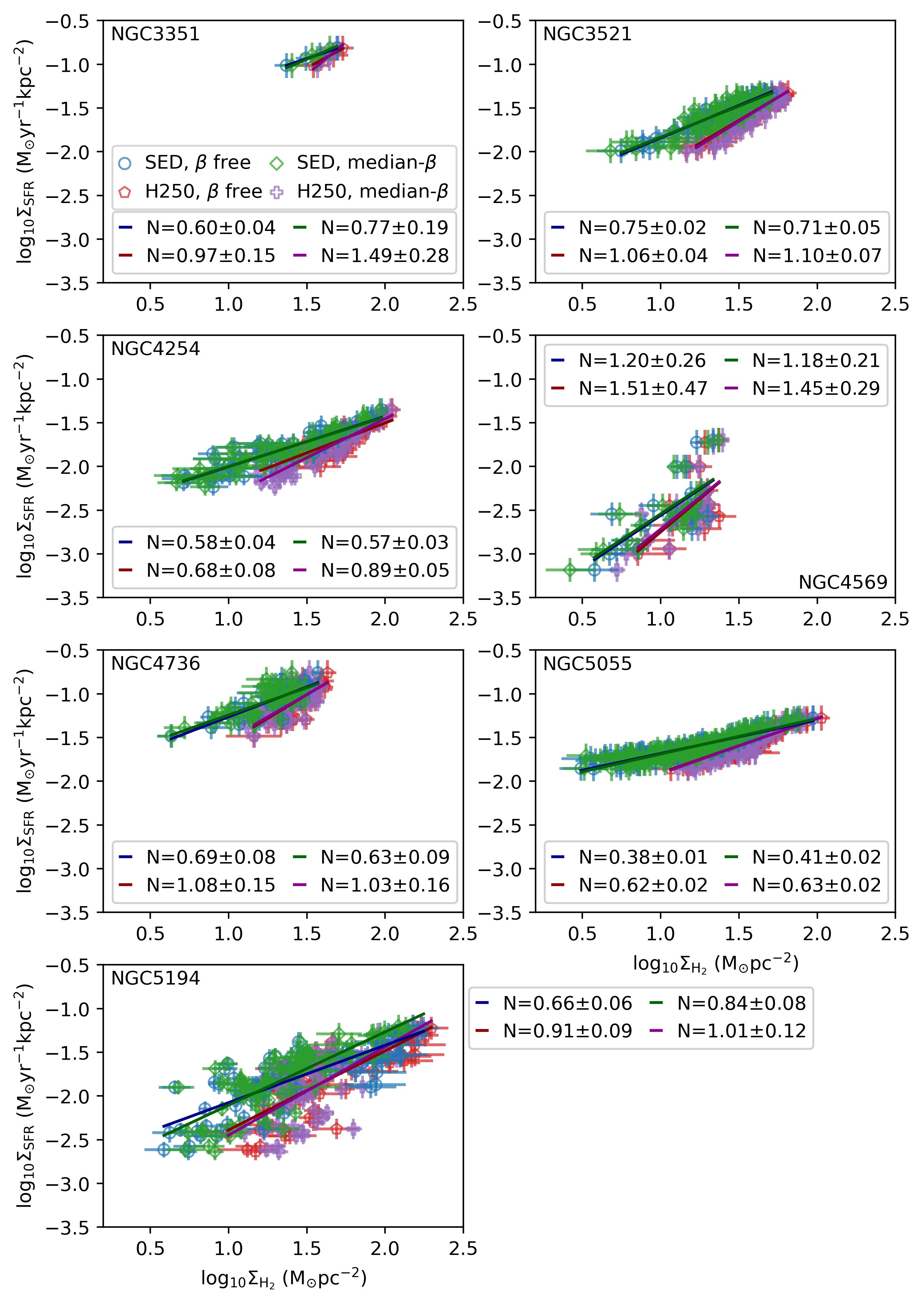
Figure 10: Resolved star formation law plots for the galaxies in our sample. Blue circles mark values of $\Sigma_{\rm H_{2}}$ derived from SED-fitted values of $\Sigma_{dust}$ with $\beta$ as a free parameter. Green diamonds; as blue circles but with $\beta$ fixed at its median value. Red pentagons mark values of $\Sigma_{\rm H_{2}}$ derived from 250$\mu$m dust emission, using values of $T$ and $\beta$ from SED fitting with $\beta$ as a free parameter. Purple pluses; as red pentagons but with $\beta$ fixed at its median value. In each case the data points are fitted with the function $\log_{10}\Sigma_{\textsc{sfr}}=N\log_{10}\Sigma_{\rm gas}+C$; best-fit lines are plotted in each panel. Best-fit relationships and correlation coefficients are listed in Table 8. All values are corrected for inclination.

We fitted the function $\log_{10}\Sigma_{\textsc{sfr}}=N\log_{10}\Sigma_{\rm H_{2}}+C$ to the data shown in Figure 10. The results of this fitting are shown in Table 8, and the best-fit lines are plotted on Figure 10.

Figure 10 shows that there is a strong correlation between dust-derived surface mass of H₂ and surface density of star formation for all of the galaxies in our sample, for both the SED-fit and the 250$\mu$m-derived values of $\Sigma_{\rm H_{2}}$. Allowing $\beta$ to vary or fixing it at its median value typically results in little difference in the best-fit indices. All of the best-fit indices are smaller than the standard KS value of $N=1.4$, with the exceptions of the 250$\mu$m median-$\beta$ fit for NGC 3351 (in which only 4 data points are fitted), and both 250$\mu$m fits for NGC 4569, in which $\Sigma_{\rm H_{2}}$ and $\Sigma_{\textsc{sfr}}$ are less well-correlated than is the case in the other galaxies in our sample. This is not a surprising result, as our submillimetre dust emission observations are tracing molecular gas surface density, rather than total gas surface density, and so a linear relationship, implying that molecular gas is converted into stars with a constant efficiency, is typically expected (e.g. Bigiel et al., 2008; Bolatto et al., 2017).

In every case, the SED-fit values of $\Sigma_{\rm H_{2}}$ produce significantly shallower values of $N$ than do the 250$\mu$m-derived values. For most of the galaxies, the SED-fit values of $N$ are somewhat sublinear, while the 250$\mu$m-derived values are broadly consistent with linearity. The exceptions are NGC 4569, in which the fitted indices are super-linear, but in which the correlation coefficients are relatively poor, and the well-correlated NGC 5055, in which the fitted indices are significantly sub-linear in both cases. There are significant offsets in $\Sigma_{\textsc{sfr}}$ between the galaxies in our sample. This is in keeping with the $\pm 0.30$ dex rms dispersion which is seen around the KS law (Kennicutt & Evans, 2012), which they note is greater than can be attributed to measurement uncertainties, and so which likely indicates physical differences in star formation rate between galaxies of comparable surface density (e.g. Ellison et al., 2021). As shown in Figure 10, the uncertainties on our values of $\Sigma_{\textsc{sfr}}$ are typically smaller than those on $\Sigma_{\rm H_{2}}$, and not subject to the uncertainty on gas-to-dust ratio which affect the $\Sigma_{\rm H_{2}}$ measurements.

6.3 Unresolved Kennicutt-Schmidt Law

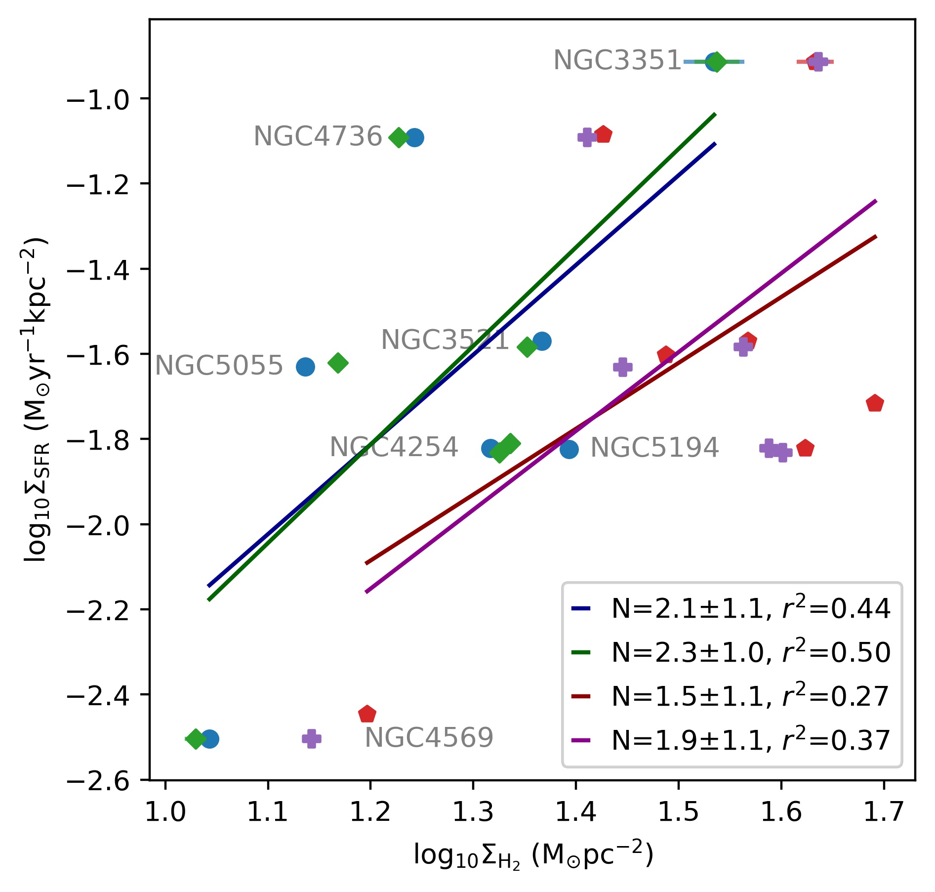
Figure 11: Mean values of $\Sigma_{\rm H_{2}}$ and $\Sigma_{\textsc{sfr}}$ for the galaxies in our sample. Lines of best-fit are plotted. Symbols and colour coding as in Figure 10.

We measured the relationship between the global values of $\Sigma_{\rm H_{2}}$ and $\Sigma_{\textsc{sfr}}$ for the galaxies in our sample. To do so, we took the mean value of $\Sigma_{\rm H_{2}}$ and $\Sigma_{\textsc{sfr}}$ for each galaxy. We are thus to some extent measuring luminosity-weighted values, although our use of SED-fitted values of $T$ and $\beta$ in our measurements of $\Sigma_{\rm H_{2}}$ should mitigate against this effect. This is intended to be analogous to observing the galaxies as unresolved sources. However, the SED-fit values of $\Sigma_{\rm H_{2}}$ remain subject to loss of extended emission: if we were truly observing unresolved sources with SCUBA-2, the full column of submillimetre emission would be accounted for. The mean values that we measure are shown in Figure 11. We see a positively correlated and broadly linear relationship between $\log_{10}(\Sigma_{\rm H_{2}})$ and $\log_{10}(\Sigma_{\textsc{sfr}})$, albeit with considerable scatter, for all four of the methods of measuring $\Sigma_{\rm H_{2}}$ which we consider. The mean values of $\Sigma_{\rm H_{2}}$ are consistently lower for the SED-fit cases than for the 250$\mu$m-derived cases, as would be expected due to the loss of large-scale emission in the SCUBA-2 data. Allowing $\beta$ to vary or fixing it at its median value produces little difference in the mean values of $\Sigma_{\rm H_{2}}$. The best-fit indices are $N_{\rm SED,\beta-free}=2.1\pm 1.1$, $N_{\rm SED,median-\beta}=2.3\pm 1.0$, $N_{\rm 250\mu m,\beta-free}=1.5\pm 1.1$, and $N_{\rm 250\mu m,median-\beta}=1.9\pm 1.1$. These values are steeper than those seen within the galaxies, and are consistent both with one another and with the KS value of $N=1.4$ within their large uncertainties. The best-fit relationships are plotted on Figure 11.

7 Discussion

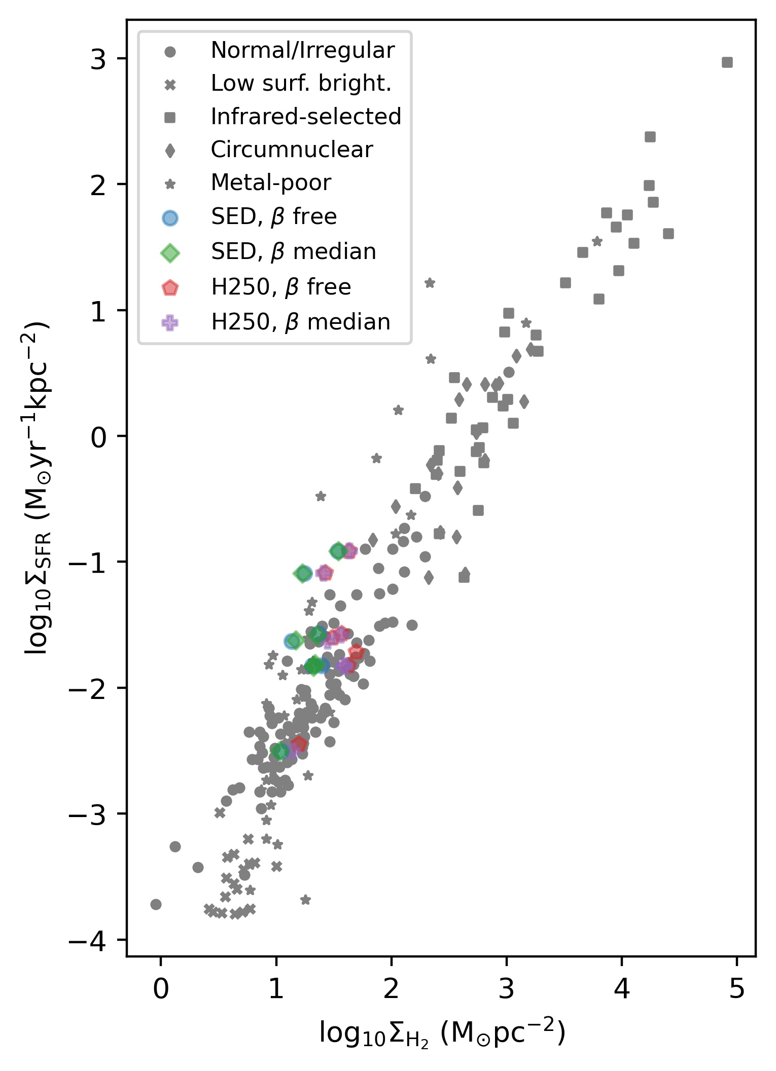
Figure 12: The mean values of $\Sigma_{\rm H_{2}}$ and $\Sigma_{\textsc{sfr}}$ for the galaxies in our sample, compared to archival measurements. The grey circles mark normal or irregular galaxies presented by Gavazzi et al. (2003), James et al. (2004), Hameed & Devereux (2005) and Kennicutt et al. (2008). Grey crosses mark the low-surface-brightness subset of these galaxies. Grey squares mark infrared-selected starburst galaxies presented by Scoville et al. (2000) and Dopita et al. (2002). Grey diamonds mark the circumnuclear starbursts presented by Kormendy & Kennicutt (2004). Grey stars mark any low-metallicity galaxies in the above samples, i.e., those where $Z<0.3\,Z_{\odot}$.

7.1 Resolved KS Law

The fact that the values of $N$ for the SED-fit cases are consistently shallower than the 250$\mu$m-derived values indicates that the atmospheric filtering to which SCUBA-2 is subject results in the loss of a higher fraction of emission in low-surface-brightness regions. This is as expected, as it is extended emission that is preferentially lost in the filtering process, as discussed in Section 2. Figure 10 shows good agreement between the SED-fit and 250$\mu$m-derived values of $\Sigma_{\rm H_{2}}$ in the highest-density regions.

If the sub-linear values of $N$ recovered from the SED-fit cases were physical, it would suggest that star formation becomes less efficient at high gas densities (e.g. Ford et al., 2013). It appears likely that the shallow indices seen in the SED-fit data typically result from spatially-filtered dust emission data being compared to $\Sigma_{\textsc{sfr}}$ maps derived from GALEX and Spitzer data, the extended components of which have not been correspondingly lost to atmospheric filtering. Nonetheless, the SED-fit data is well-correlated with $\Sigma_{\textsc{sfr}}$, indicating that the SCUBA-2 850$\mu$m emission is a good tracer of star formation despite missing some fraction of the extended dust emission.

The $\Sigma_{\textsc{sfr}}$ maps constructed from GALEX and Spitzer data trace star formation on timescales $\sim 5-100$ Myr (Leroy et al., 2008; Kennicutt & Evans, 2012, and refs. therein). Therefore the 250$\mu$m-derived relationship between $\Sigma_{\rm H_{2}}$ and $\Sigma_{\textsc{sfr}}$ is more accurate than the SED-fit relationship only if the gas traced by Herschel but not by SCUBA-2 will arises from molecular clouds which will form stars in the next $\sim 5-100$ Myr. Observations of local star-forming regions have shown that in resolved observations of molecular clouds SCUBA-2 effectively selects for dense and gravitationally bound material which is likely to form stars in the immediate future (Ward-Thompson et al., 2016). While each SCUBA-2 beam in our observations will integrate over many star-forming molecular cloud complexes, the strong correlation between the SED-fit $\Sigma_{\rm H_{2}}$ values and $\Sigma_{\textsc{sfr}}$ nonetheless suggests that a gas density peak sufficiently strong to be traceable by SCUBA-2 may be required for significant amounts of star formation to occur.

Most of the galaxies in our sample are, in the 250$\mu$m-derived case, broadly consistent with $N\sim 1$, suggesting a linear relationship between molecular gas mass and star formation rate (e.g. Bigiel et al., 2008; Lada et al., 2012). NGC 3351 and NGC 4569 show somewhat steeper relationships, but the former includes only four pixels in the galactic centre, and the latter is relatively weakly correlated. Uniquely in our sample, NGC 5055 shows an index which is significantly $<1$ in both the SED-fit and 250$\mu$m-derived cases, and has a very high correlation coefficient between $\Sigma_{\rm H_{2}}$ and $\Sigma_{\textsc{sfr}}$.

The indices which we derive from dust emission for the galaxies in our sample are somewhat similar to those derived from dust emission by Ford et al. (2013) for M31. Ford et al. (2013) found an index of $0.55\pm 0.01$ in M31 from Herschel dust emission, quite similar to the values which we typically measure in the SED-fit case, but shallower than the indices which we typically measure using 250$\mu$m-derived values. However, the Ford et al. (2013) value for M31 is similar to our 250$\mu$m-derived values for NGC 5055, $0.62\pm 0.02$ and $0.63\pm 0.02$, perhaps suggesting a commonality between the two galaxies. However, none of our galaxies have indices similar to that measured on kpc scales in M33 from dust emission by (Williams et al., 2018), of $5.85\pm 2.37$.

The broadly linear relationship between 250$\mu$m-derived $\Sigma_{\rm H_{2}}$ and $\Sigma_{\textsc{sfr}}$ suggests that the molecular clouds or cloud complexes traced by Herschel will go on to form stars on timescales $\sim 5-100$ Myr. The star formation efficiency per freefall time of a molecular cloud is very low ($\sim 1$%; e.g., McKee & Ostriker 2007), and so we expect only a very small fraction of the material traced by these observations to be incorporated into new stars on this timescale. However, the equally good, albeit sub-linear, correlation between the SED-fit $\Sigma_{\rm H_{2}}$ and $\Sigma_{\textsc{sfr}}$ suggests that SCUBA-2 is also a good tracer of star formation.

The fact that 250$\mu$m-derived $\Sigma_{\rm H_{2}}$ and SED-fit $\Sigma_{\rm H_{2}}$ are equally well-correlated with $\Sigma_{\textsc{sfr}}$ suggests that the relatively diffuse material traced by Herschel but not by SCUBA-2 is (a) not forming stars independently of the material traced by SCUBA-2 and (b) associated with the same star-forming peaks in column density which are detected by SCUBA-2. We suggest that SCUBA-2 is preferentially detecting the denser material within these molecular clouds. We hypothesise that this denser material may be likely to form stars on a timescale shorter than that of the material exclusively traced by Herschel.

7.2 Unresolved KS law

Figure 11 shows that the best-fit index for the star formation law over the mean values $\langle\Sigma_{\rm H_{2}}\rangle$ and $\langle\Sigma_{\textsc{sfr}}\rangle$ of our sample of galaxies is steeper, and more comparable to the standard KS value of $N=1.4$, than are those in the individual galaxies shown in Figure 10, although the uncertainties on the fits are sufficiently large that the comparison may not be meaningful. The fitted values are also broadly consistent with linearity, as would be expected for tracers of molecular gas (Gao & Solomon, 2004). The presence or absence of the full column of dust emission changes only the offset of the slope and not the slope itself, again to within the very large uncertainties on the fit. This again suggests that the presence of a SCUBA-2 detection is a good predictor of star formation. We emphasise that the loss of the contribution from extended emission in the SCUBA-2 data affects these results because we are averaging over observations of resolved sources; if we were observing more distant unresolved galaxies, the full column of submillimetre emission would be accounted for.

We note that in this paper we have assumed a single gas-to-dust ratio and mean molecular mass for all of the galaxies in our sample. Some amount of the scatter in $\langle\Sigma_{\rm H_{2}}\rangle$ seen in Figure 11 could thus be caused by systematic errors in the conversion from dust to gas mass. However, the variations in metallicity in our sample are not large (see Table 1), suggesting that not all of the observed scatter is due to errors in in this conversion.

We compared our results to archival measurements of a range of galaxies in Figure 12. Our galaxies correspond well to the normal/irregular galaxies presented by Gavazzi et al. (2003), James et al. (2004), Hameed & Devereux (2005) and Kennicutt et al. (2008). This is as expected, as all of the galaxies for which we have calculated $\Sigma_{\textsc{sfr}}$ are non-starbust spirals. The SED-fit values – in which the extended component of the SFR tracers is included but that of the dust emission is not – correspond better to the metal-poor archival galaxies ($Z/Z_{\odot}<0.3$) than to the ‘normal’ sample. Although the galaxies which we consider have sub-solar metallicities, the lowest-metallicity galaxy, NGC 4254, has $Z/Z_{\odot}=0.72$ (De Vis et al., 2019). Using the 250$\mu$m-derived data puts the galaxies in our sample in the midst of the normal galaxies. This is as expected because, as discussed above, if dust continuum emission is lost to atmospheric filtering, the dust mass derived for the galaxy will be systematically lowered, and the galaxy will artificially appear metal-poor. Feathering of JCMT data with lower-resolution Planck or Herschel data (Smith et al., 2021) could aid in direct comparison of the cold dust and star formation tracers.

8 Summary

In this paper we have presented 850$\mu$m dust continuum observations of 8 nearby galaxies made with the SCUBA-2 camera on the James Clerk Maxwell Telescope (JCMT) as part of the JCMT Nearby Galaxies Legacy Survey (NGLS). The galaxies which we present are NGC 3034, NGC 3351, NGC 3521, NGC 4254, NGC 4569, NGC 4736, NGC 5055 and NGC 5194. These galaxies were selected for their high surface brightness and the presence of ancillary data, and are not a representative sample of local galaxies.

We find that there is a significant contribution from the ¹²CO $J=3\to 2$ line in the SCUBA-2 850$\mu$m observations of all of the galaxies in our sample, typically $\sim 20$%, but higher for NGC 3034 and NGC 5194. We corrected the SCUBA-2 maps for this CO contamination using NGLS HARP ¹²CO $J=3\to 2$ observations.

Comparison of our observations to VLA Hi and Nobeyama 45m ¹²CO $J=1\to 0$ observations shows that SCUBA-2 850$\mu$m emission is correlated with ¹²CO emission, suggesting that the dust emission detected by SCUBA-2 is tracing molecular hydrogen gas. SCUBA-2 850$\mu$m emission is not well-correlated with atomic hydrogen emission.

We fitted spectral energy distributions to each of the galaxies in our sample in order to measure surface dust mass, dust temperature and dust opacity index, using our SCUBA-2 850$\mu$m data and archival Herschel Space Observatory observations. To do this, we filtered the Herschel data to match the spatial scales present in the SCUBA-2 data. For our chosen SCUBA-2 data reduction scheme, a large fraction of the Herschel emission (a mean of 58%) was lost, principally the extended, low-surface-brightness component.

We constructed resolved and unresolved star formation law plots for 7 of the galaxies in our sample, using archival Spitzer and GALEX data to measure surface density of star formation.

In the resolved case, we found that comparing surface density of star formation rate ($\Sigma_{\textsc{sfr}}$) to SED-fit-derived (i.e. subject to atmospheric filtering) values of H₂ surface density ($\Sigma_{\rm H_{2}}$) typically produces sublinear star formation law indices, while comparing to Herschel 250$\mu$m-derived values typically produces indices which are broadly linear. The exceptions to this are the poorly-fitted NGC 4569, which is significantly superlinear in both cases, and the well-fitted NGC 5055, which is significantly sublinear in both cases. The Herschel 250$\mu$m-derived star formation law index for NGC 5055 is similar to that found in M31 by Ford et al. (2013), suggesting a commonality between the two galaxies.

In the unresolved case, we found that comparing the mean values of $\Sigma_{\textsc{sfr}}$ and $\Sigma_{\rm H_{2}}$ of the galaxies in our sample returns star formation law indices which are broadly consistent with both the Kennicutt-Schmidt value of 1.4 and linearity, within the large error bars on the best-fit indices. The loss of large-scale emission in the SCUBA-2 data changes the offset, but not the measured index, of the star formation law measured across the galaxies in our sample. The galaxies which we consider have mean $\Sigma_{\textsc{sfr}}$ and $\Sigma_{\rm H_{2}}$ values consistent with their being ‘normal’ spiral galaxies, when compared to archival measurements.

We find that SCUBA-2 emission is very well-correlated with star formation, but that SCUBA-2 cannot capture the extended dust emission component of the galaxies in our sample. We suggest that Herschel emission traces material in molecular clouds which will form stars on timescales comparable to the star formation timescale traced by GALEX and Spitzer data, while SCUBA-2 preferentially traces the densest gas within these clouds, which we hypothesise may form stars on a shorter timescale.

Data Availability

The raw SCUBA-2 data used in this paper are available in the JCMT archive at the Canadian Astronomy Data Centre under project code MJLSN07. The reduced SCUBA-2 data presented in this paper are available at https://dx.doi.org/10.11570/23.0007.

Appendix A Comparison of gas and dust emission

In this appendix we present comparisons of SCUBA-2 850$\mu$m surface brightness to atomic and molecular hydrogen column density, derived from VLA Hi and Nobeyama 45m ¹²CO $J=1\to 0$ data respectively, as described in Section 4.

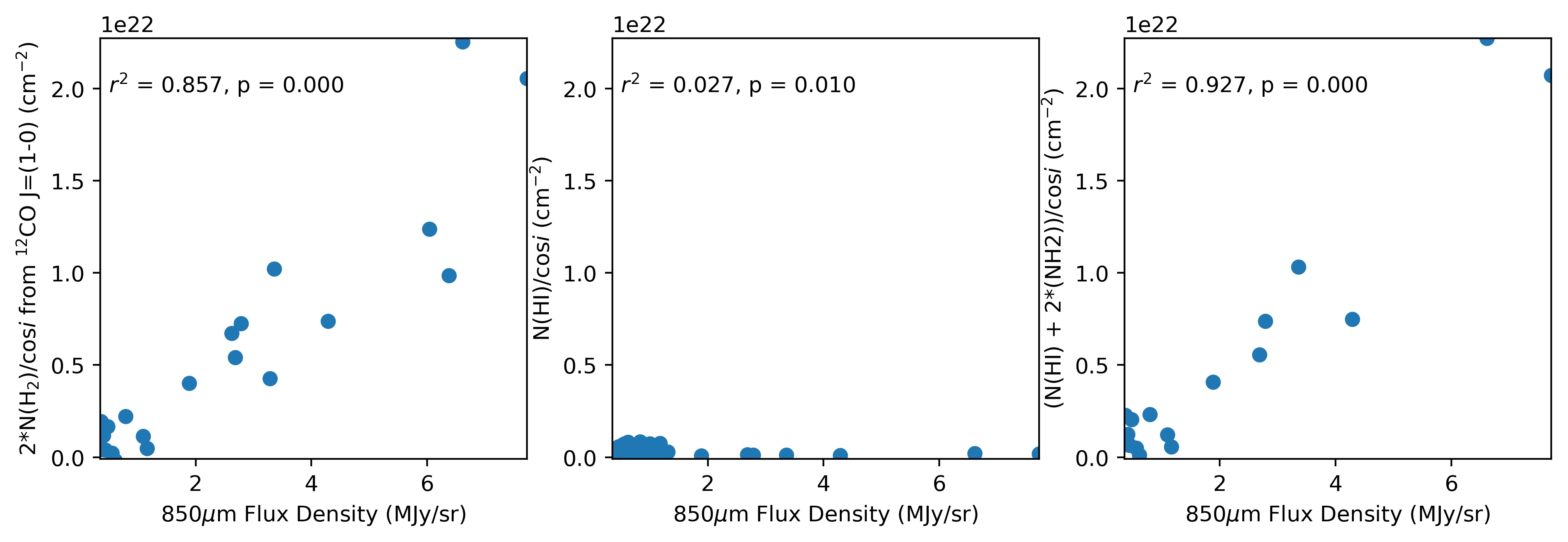
Figure 14: Comparison of dust and gas emission in NGC 3351. Panels as in Figure 13.

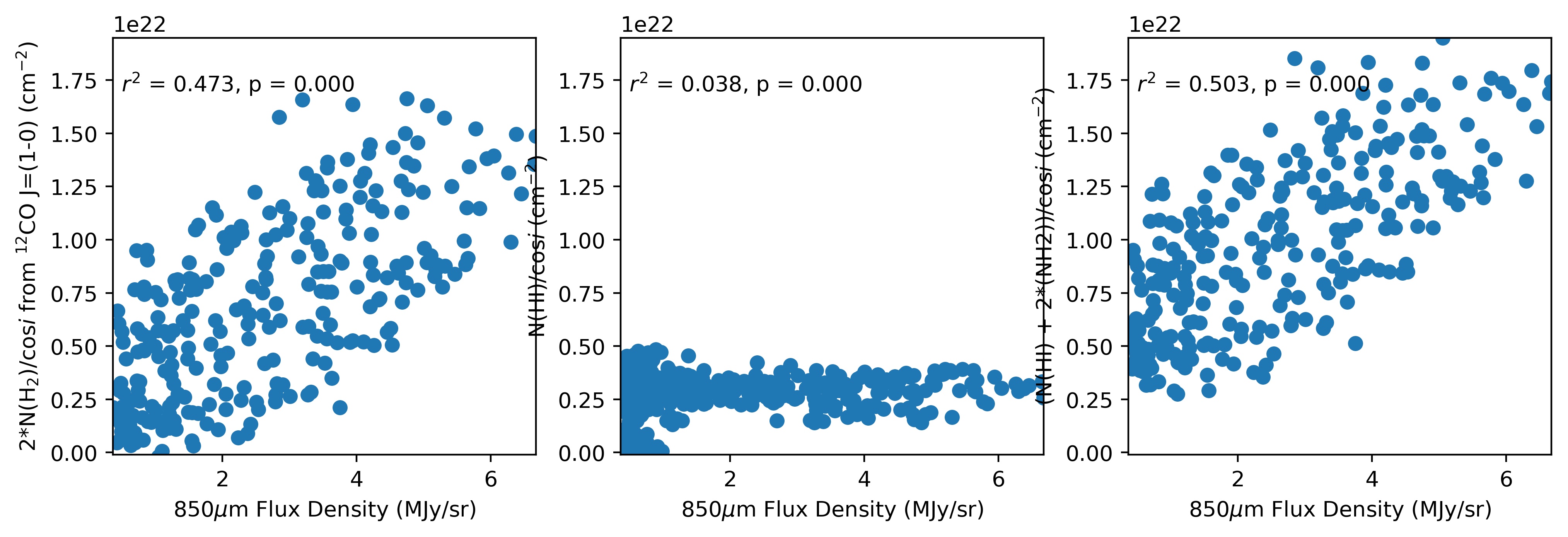
Figure 15: Comparison of dust and gas emission in NGC 3521. Panels as in Figure 13.

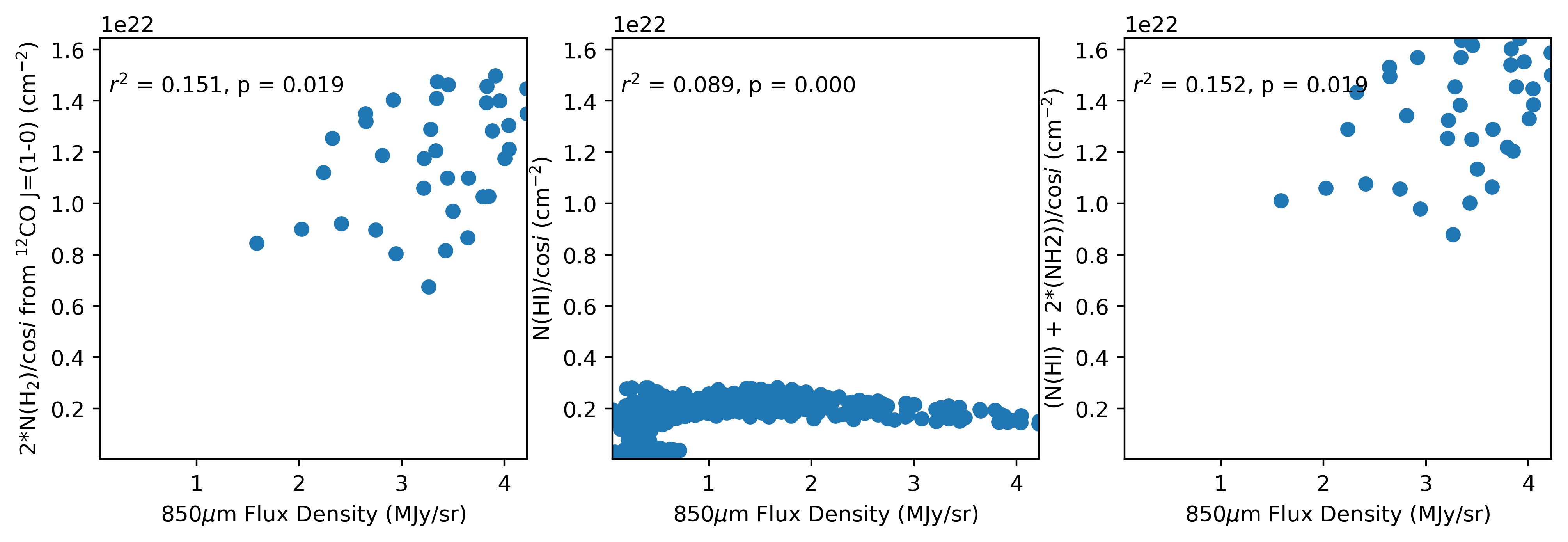
Figure 16: Comparison of dust and gas emission in NGC 4254. Panels as in Figure 13.

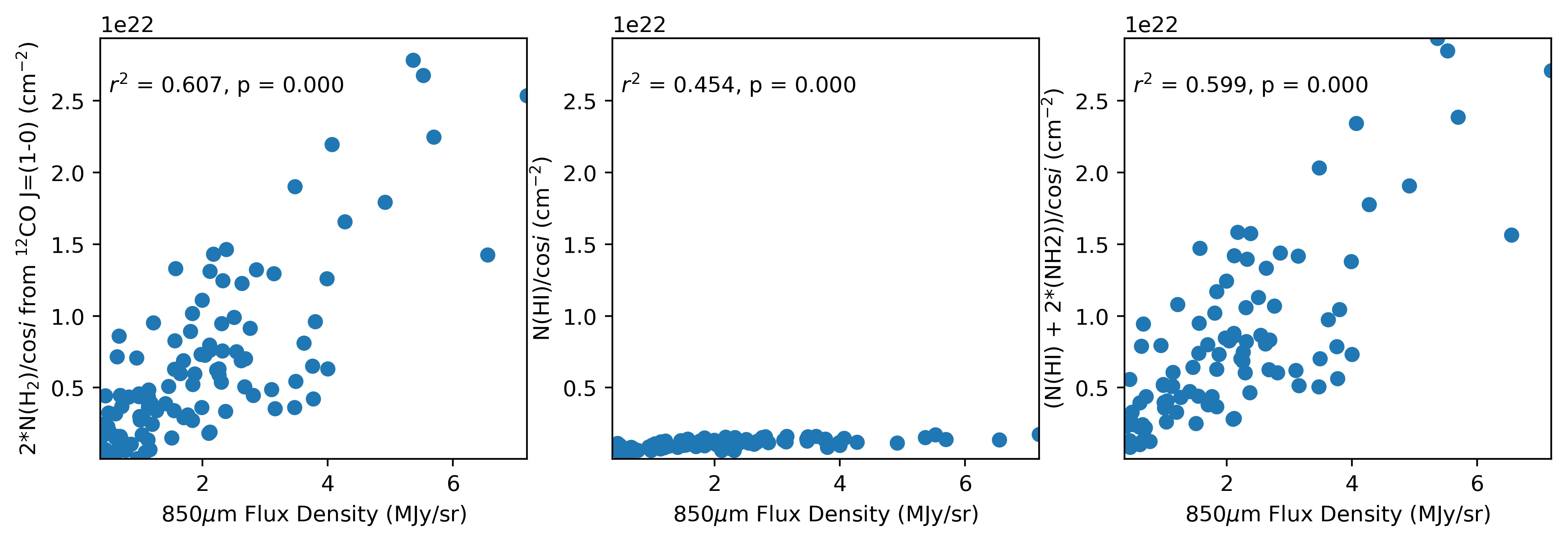
Figure 17: Comparison of dust and gas emission in NGC 4569. Panels as in Figure 13.

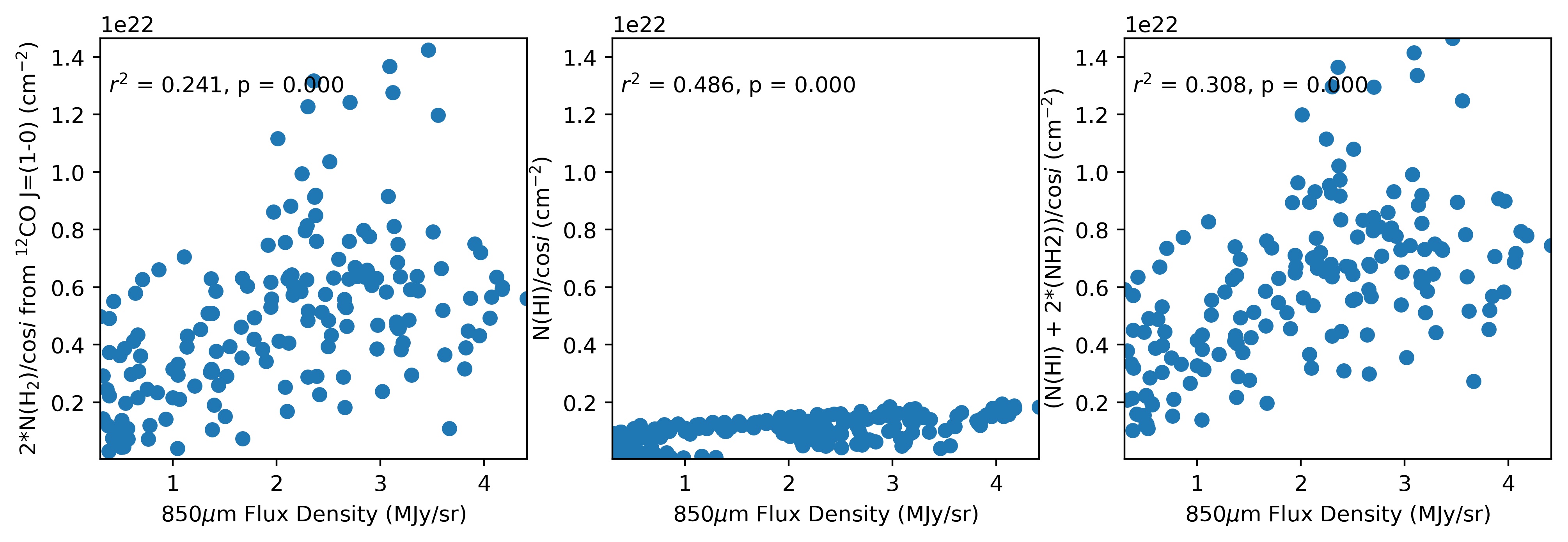
Figure 18: Comparison of dust and gas emission in NGC 4736. Panels as in Figure 13.

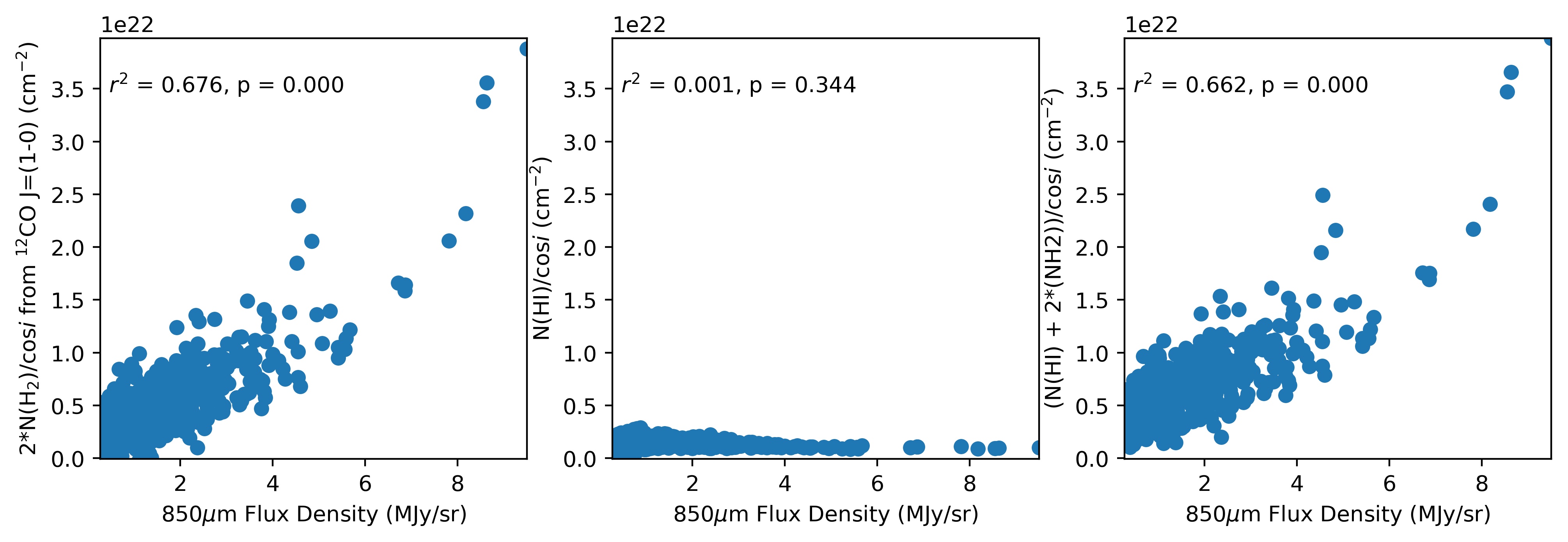
Figure 19: Comparison of dust and gas emission in NGC 5055. Panels as in Figure 13.

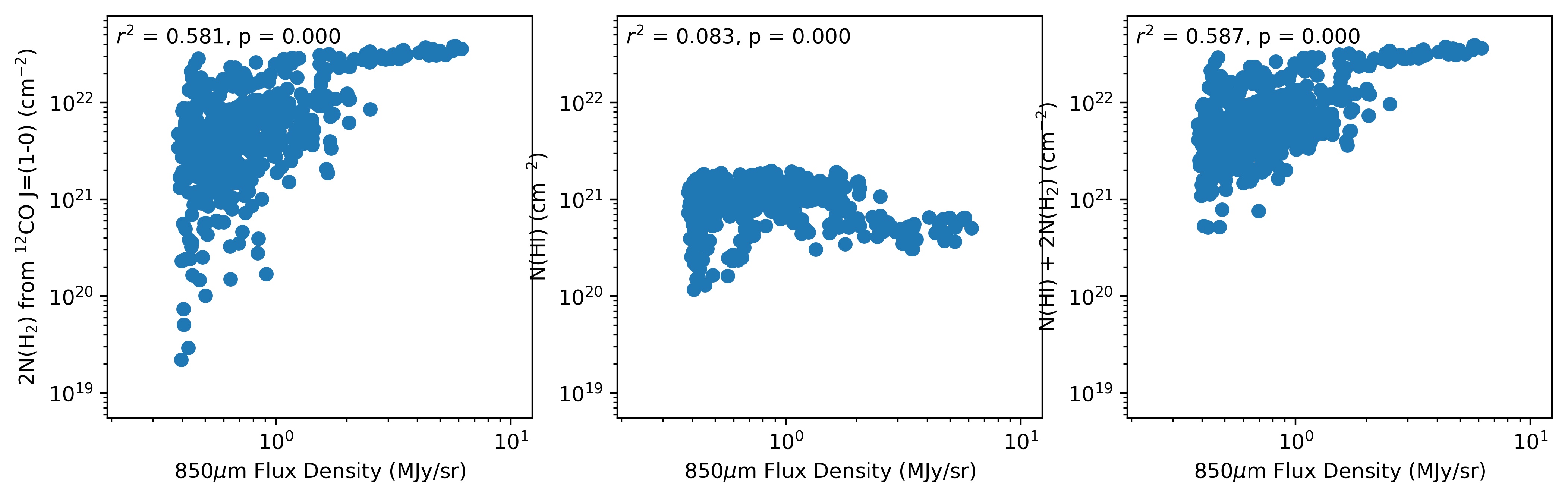
Figure 20: Comparison of dust and gas emission in NGC 5194. Panels as in Figure 13.

Appendix B SED fitting

In this appendix we present maps of molecular hydrogen column density $N({\rm H}_{2})$, dust temperature $T$ and dust opacity index $\beta$ resulting from the SED fitting described in Section 5. All maps are shown at a common resolution of 25.2^′′.

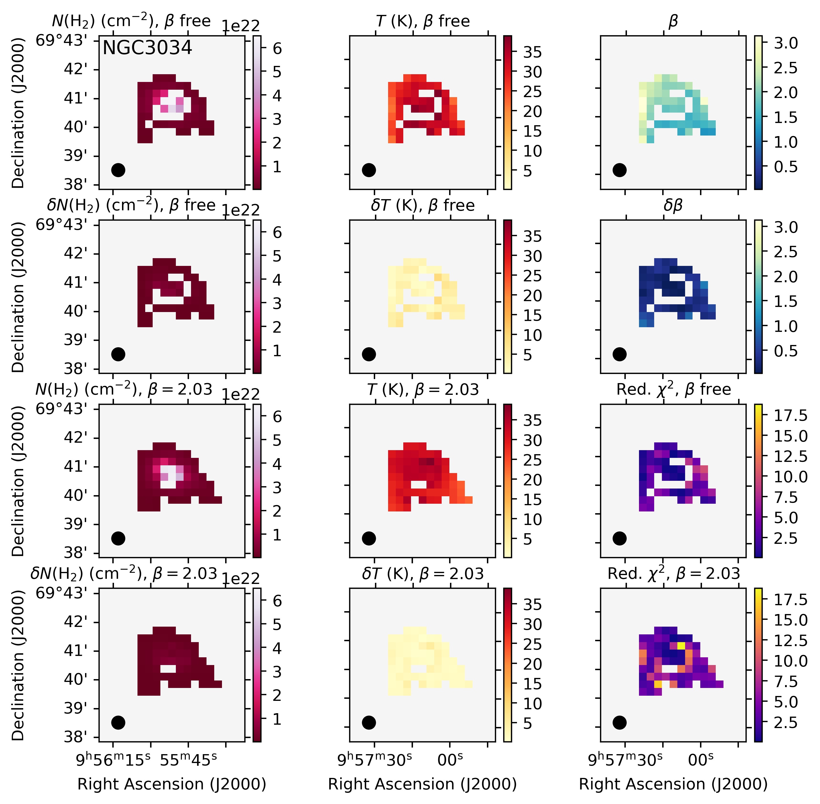
Figure 21: SED fitting results for NGC3034. Left column: top, column density $N({\rm H}_{2})$ in cm^-2, $\beta$-free case; upper centre, uncertainty on $N({\rm H}_{2})$, $\beta$-free case; lower centre, $N({\rm H}_{2})$, median-$\beta$ case; bottom, uncertainty on $N({\rm H}_{2})$, median-$\beta$ case. Centre column: top, dust temperature $T$ in K, $\beta$-free case; upper centre, uncertainty on $T$, $\beta$-free case; lower centre, $T$, median-$\beta$ case; bottom, uncertainty on $T$, median-$\beta$ case. Right column: top, dust opacity index $\beta$, $\beta$-free case; upper centre, uncertainty on $\beta$, $\beta$-free case; lower centre, reduced $\chi^{2}$ values, $\beta$-free case; bottom, reduced $\chi^{2}$ values, median-$\beta$ case.

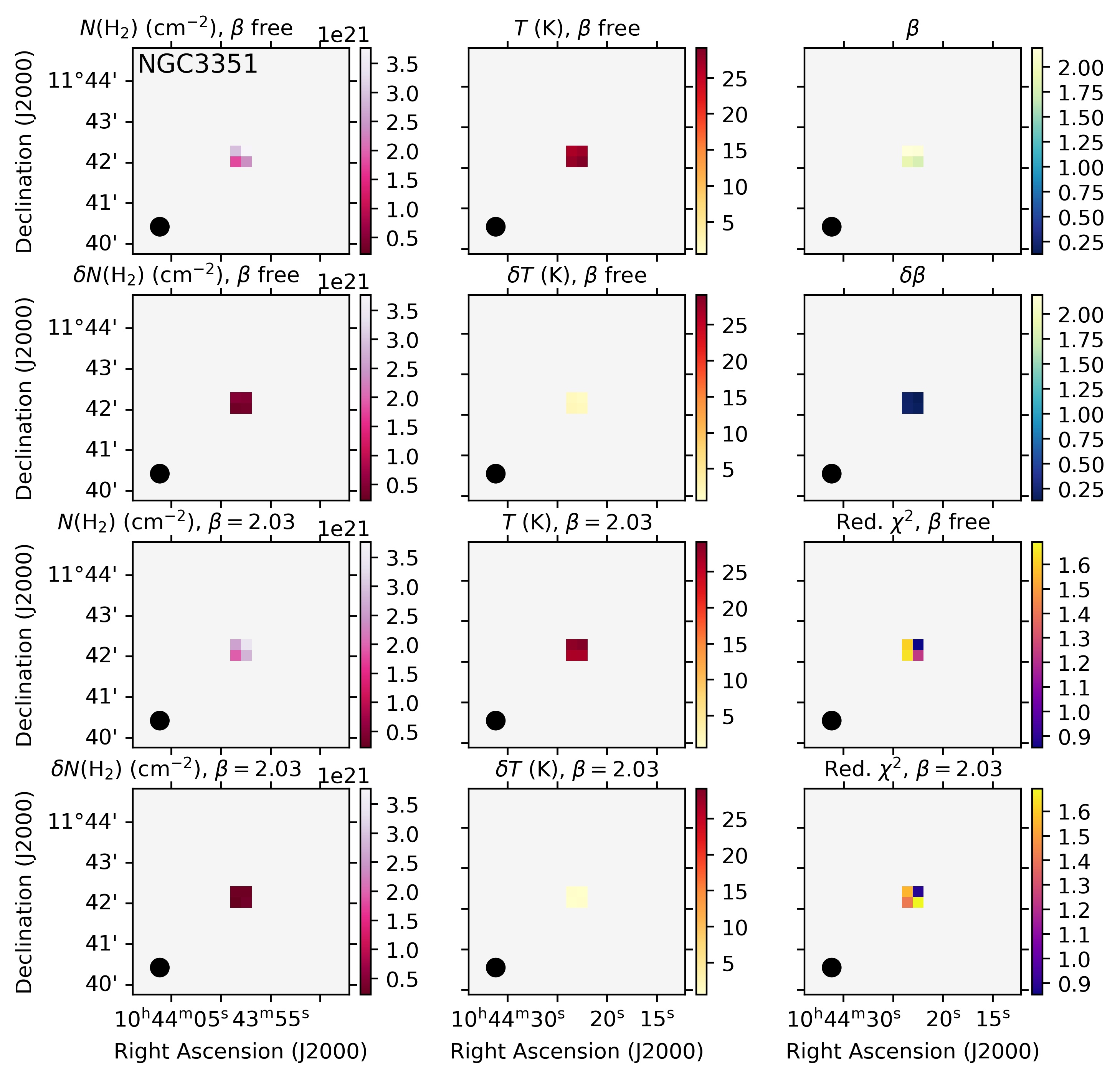
Figure 22: SED fitting results for NGC3351. Panels as in Figure 21.

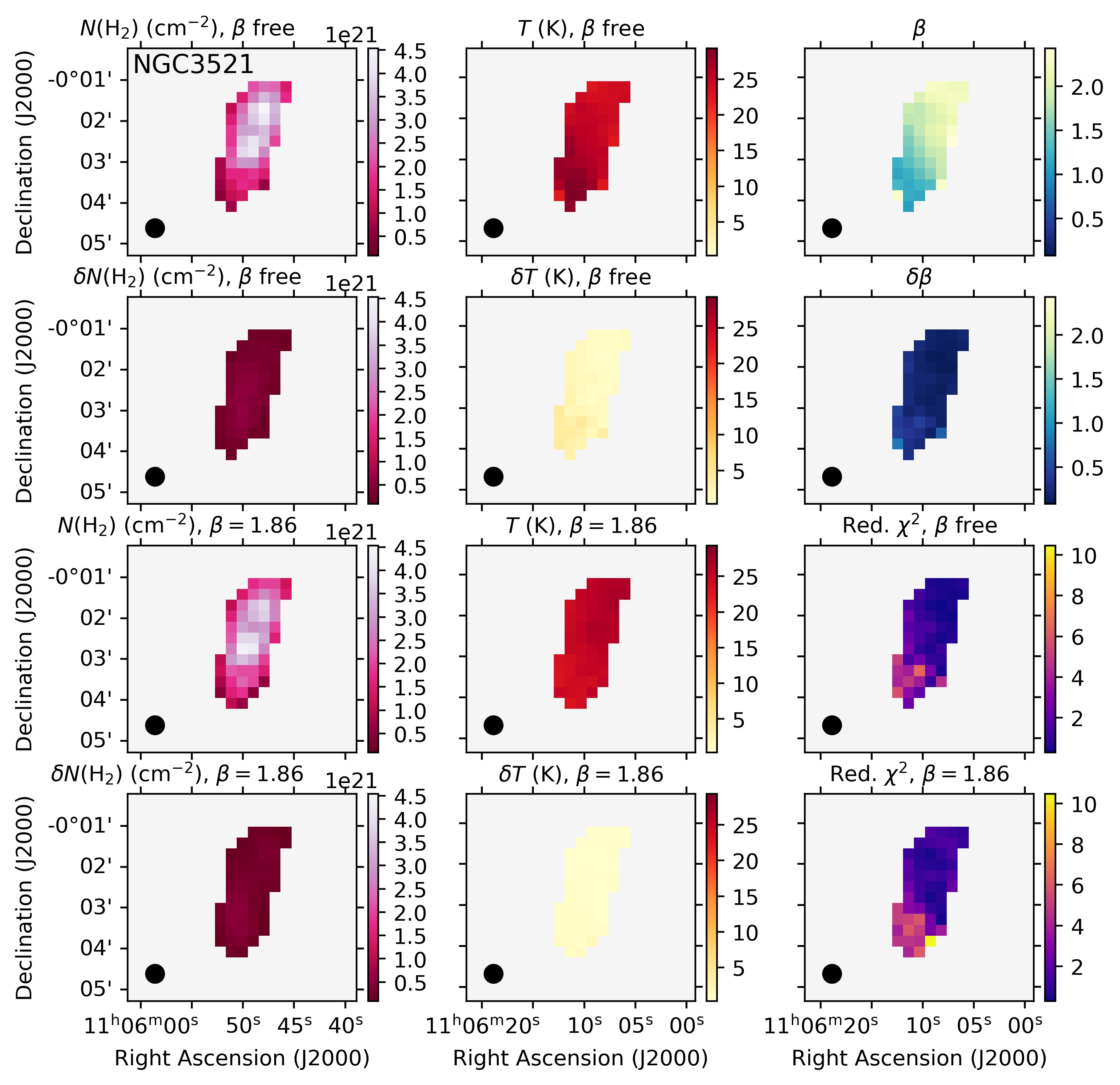
Figure 23: SED fitting results for NGC3521. Panels as in Figure 21.

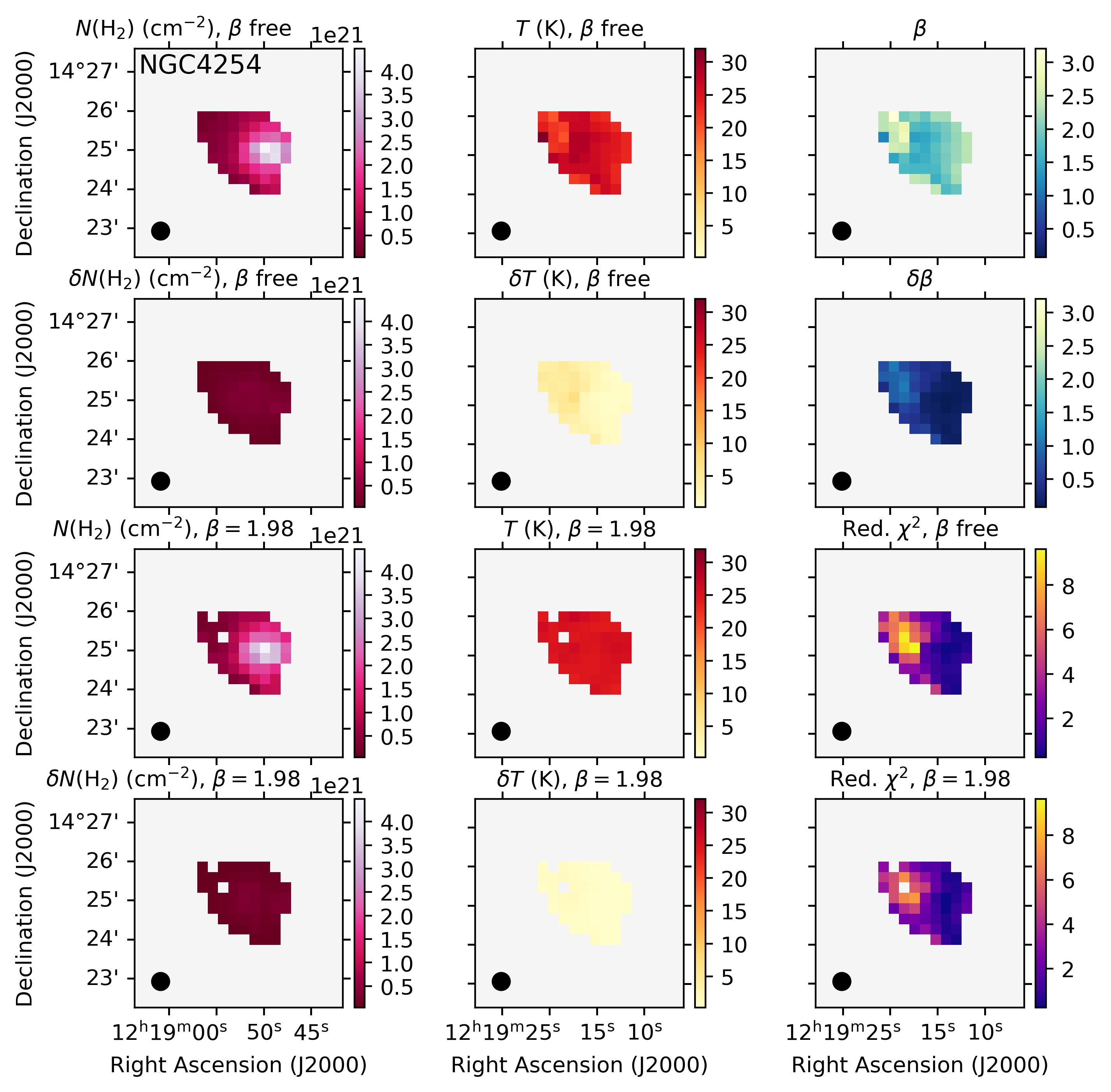
Figure 24: SED fitting results for NGC4254. Panels as in Figure 21.

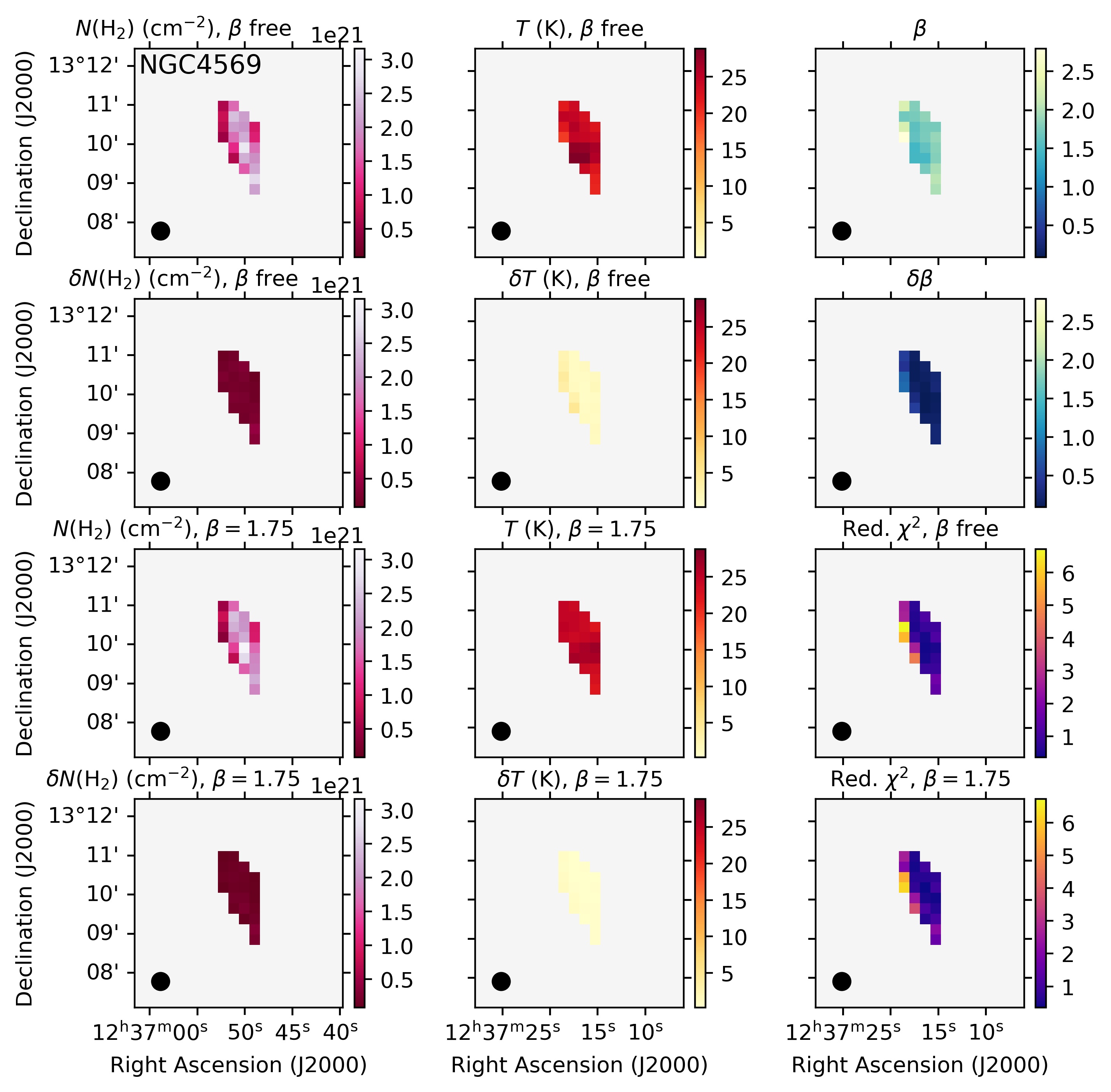
Figure 25: SED fitting results for NGC4569. Panels as in Figure 21.

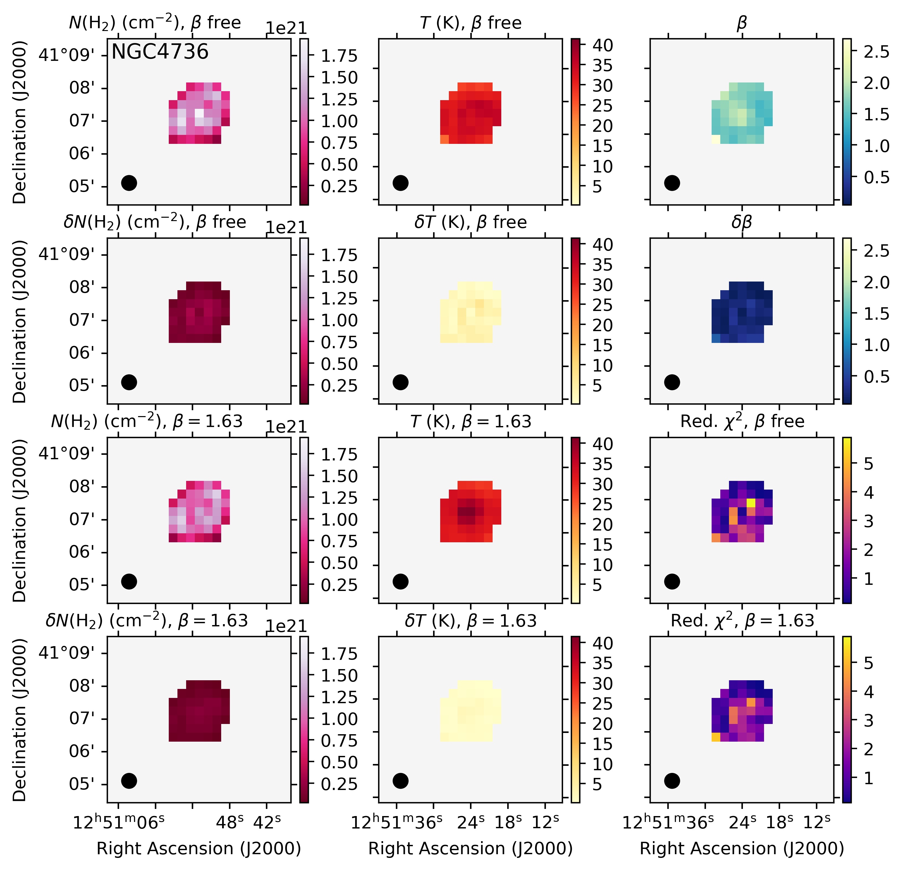
Figure 26: SED fitting results for NGC4736. Panels as in Figure 21.

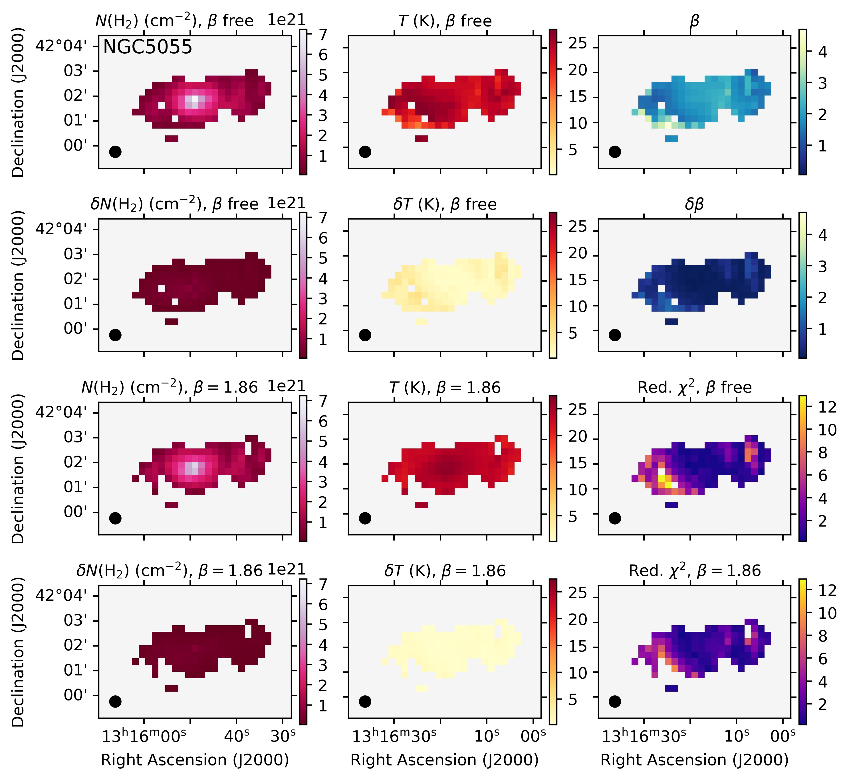
Figure 27: SED fitting results for NGC5055. Panels as in Figure 21.

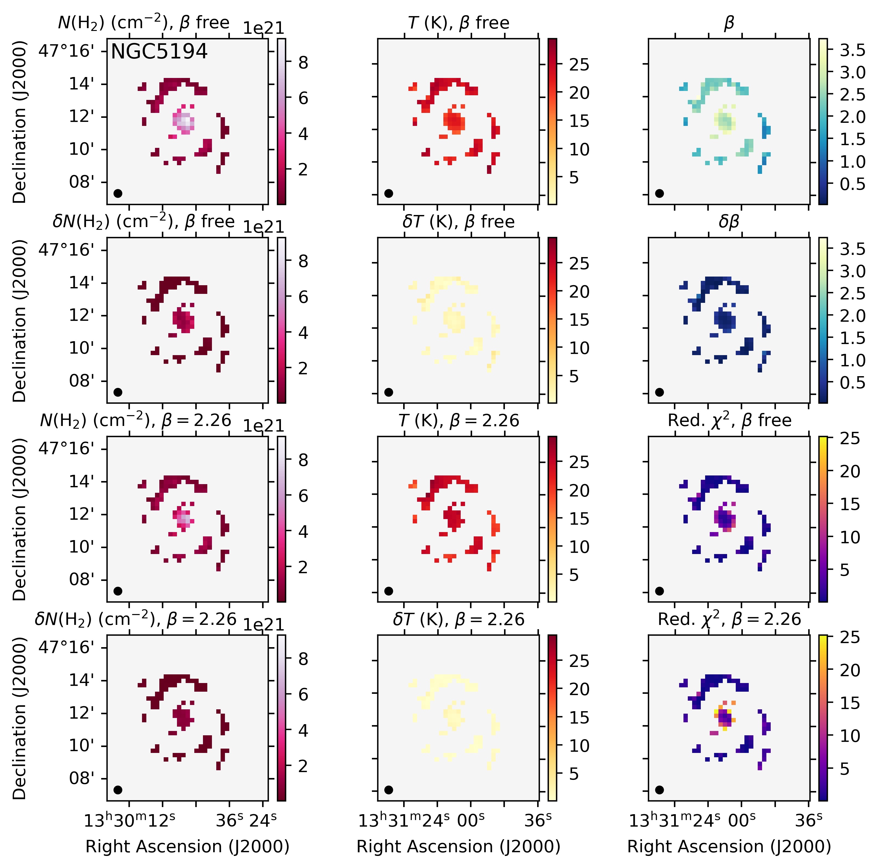
Figure 28: SED fitting results for NGC5194. Panels as in Figure 21.

Appendix C Multiwavelength imaging

In this appendix we present Spitzer 24$\mu$m, Spitzer 3.6$\mu$m, GALEX FUV and GALEX NUV imaging of each of the galaxies in our sample, taken from the Dustpedia database (Clark et al., 2018).

Appendix D Star formation rates

In this appendix we present the GALEX FUV, Spitzer 24$\mu$m, Spitzer 3.6$\mu$m and star formation surface density maps for each galaxy in our sample, except NGC 3034, as described in Section 6.1. All maps are shown at a common resolution of 25.2^′′.

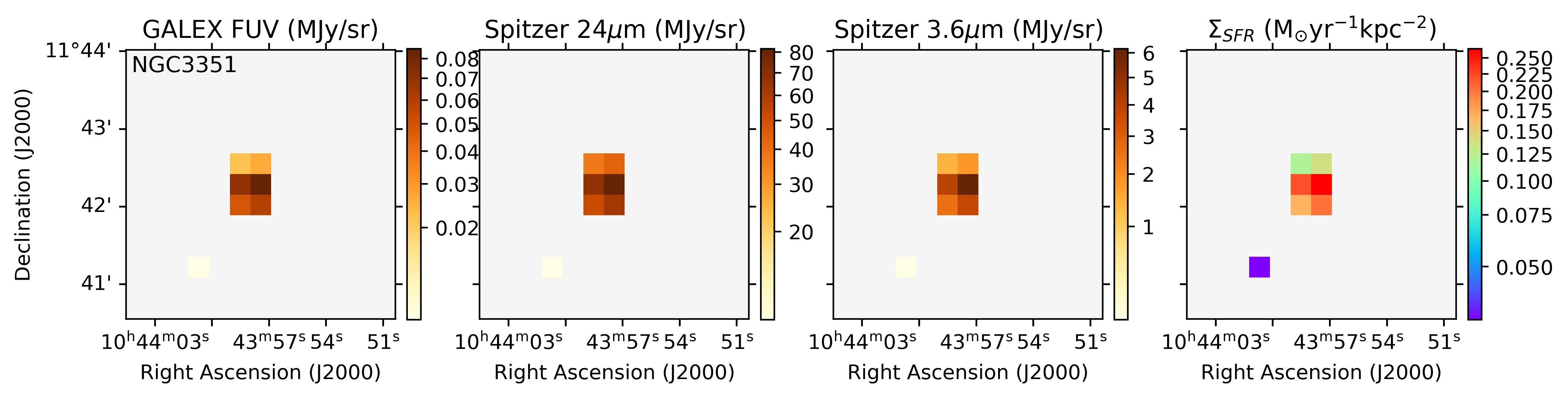
Figure 37: Surface density of star formation in NGC 3351. Far left: GALEX FUV surface brightness; centre left: Spitzer 24$\mu$m surface brightness; centre right: Spitzer 3.6$\mu$m surface brightness. All are taken from the Dustpedia database (Clark et al., 2018), and smoothed to $25\aas@@fstack{\prime\prime}2$ resolution and gridded to 16^′′ pixels. Far right: surface density of star formation.

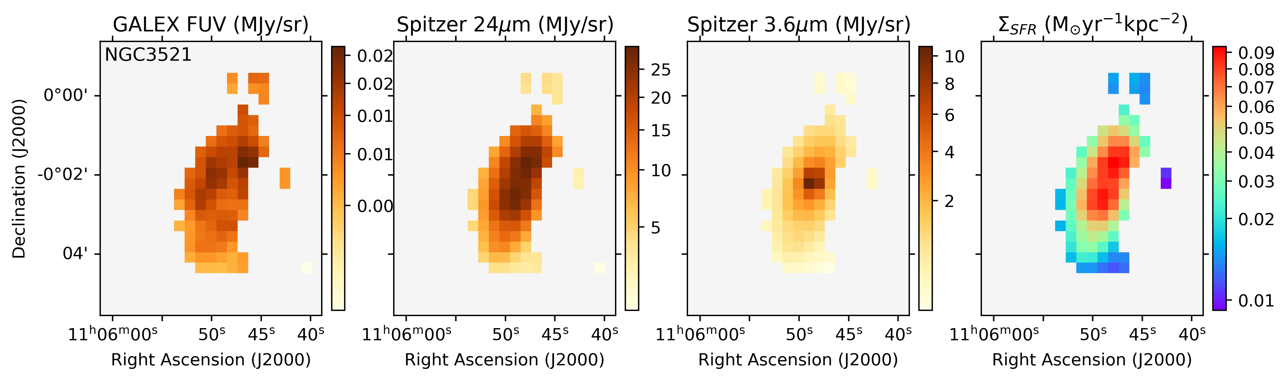
Figure 38: Surface density of star formation in NGC 3521. Panels as in Figure 37.

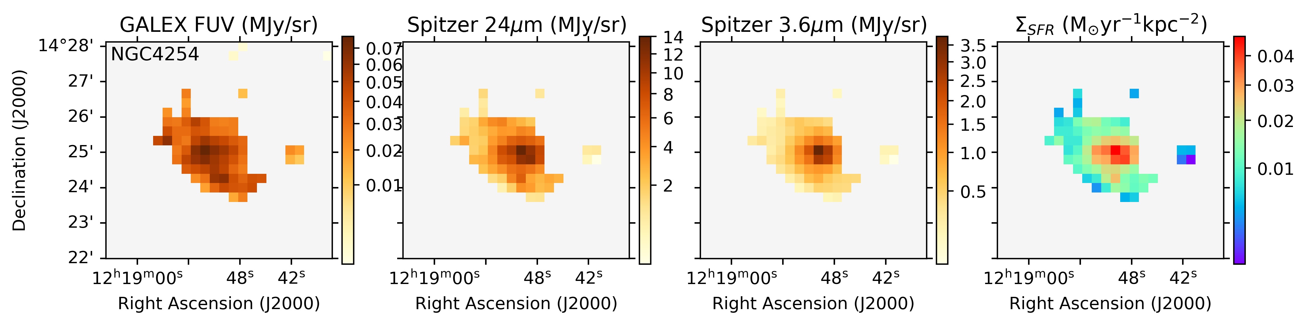
Figure 39: Surface density of star formaiton in NGC 4254. Panels as in Figure 37.

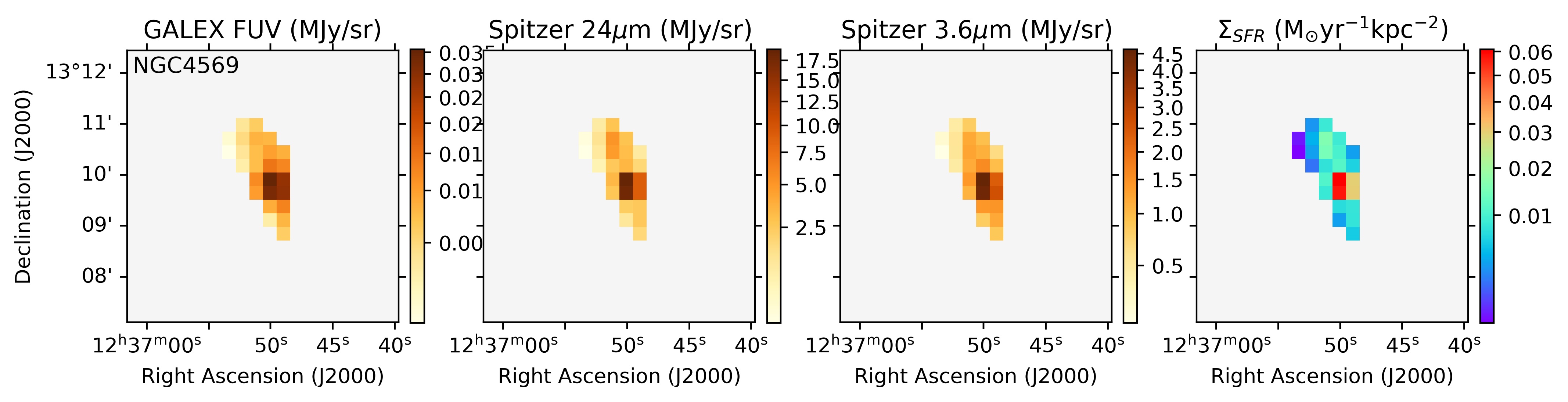
Figure 40: Surface density of star formation in NGC 4569. Panels as in Figure 37.

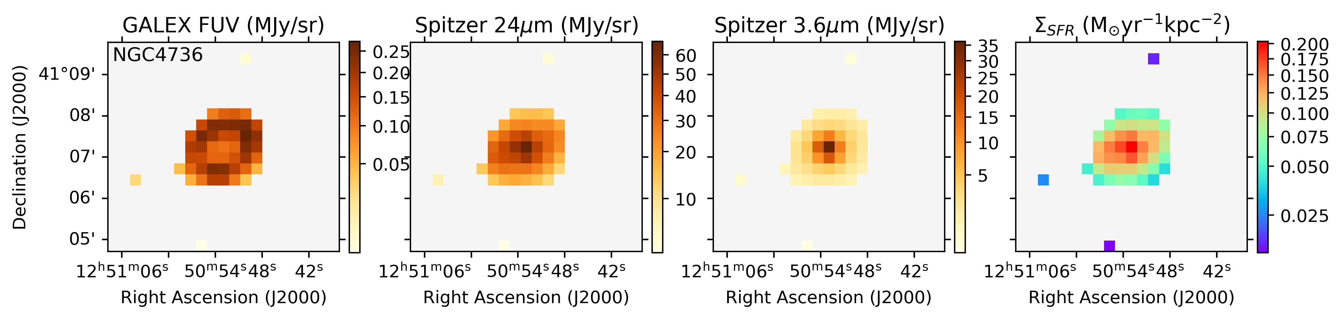
Figure 41: Surface density of star formation in NGC 4736. Panels as in Figure 37.

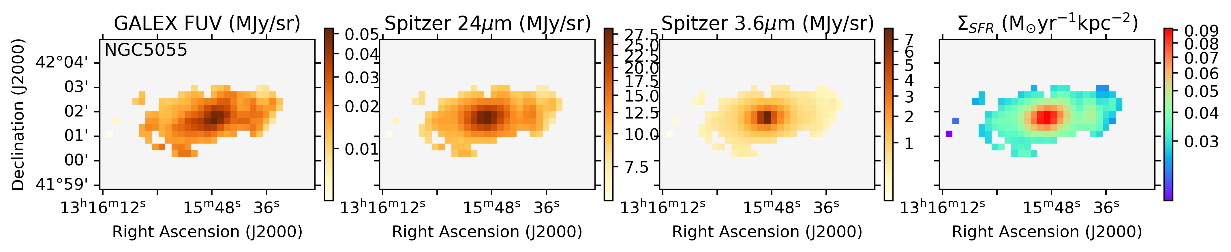
Figure 42: Surface density of star formation in NGC 5055. Panels as in Figure 37.

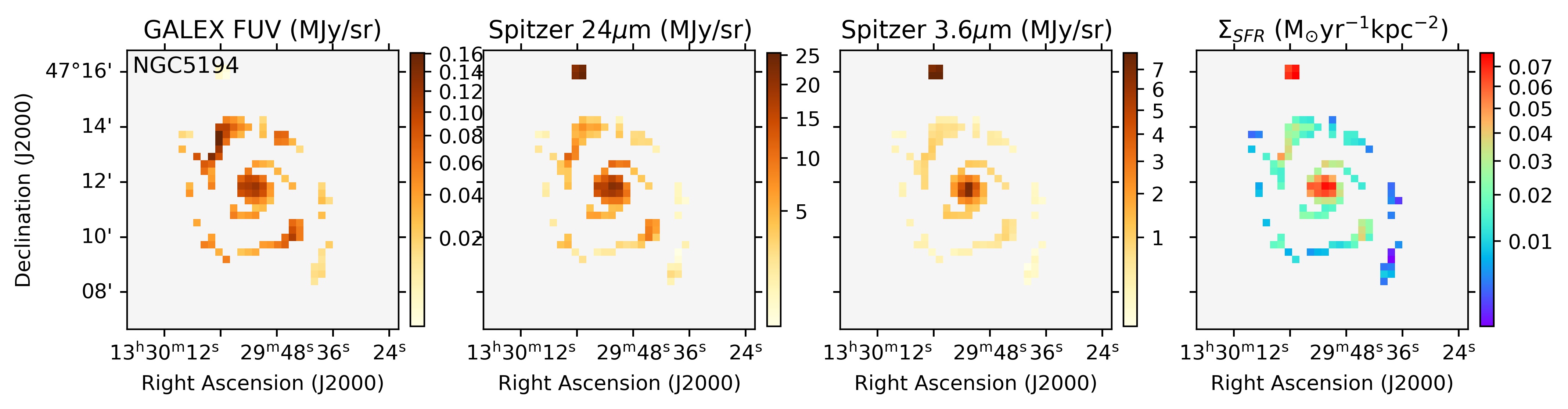
Figure 43: Surface density of star formation in NGC 5194. Panels as in Figure 37.

References

- Alloin & Nieto (1982) Alloin D., Nieto J. L., 1982, A&AS, 50, 491
- Asplund et al. (2009) Asplund M., Grevesse N., Sauval A. J., Scott P., 2009, ARA&A, 47, 481
- Battaglia et al. (2006) Battaglia G., Fraternali F., Oosterloo T., Sancisi R., 2006, A&A, 447, 49
- Bergin & Tafalla (2007) Bergin E. A., Tafalla M., 2007, ARA&A, 45, 339
- Bigiel et al. (2008) Bigiel F., Leroy A., Walter F., Brinks E., de Blok W. J. G., Madore B., Thornley M. D., 2008, AJ, 136, 2846
- Bolatto et al. (2013) Bolatto A. D., Wolfire M., Leroy A. K., 2013, ARA&A, 51, 207
- Bolatto et al. (2017) Bolatto A. D., et al., 2017, ApJ, 846, 159
- Boselli et al. (2016) Boselli A., et al., 2016, A&A, 587, A68
- Buckle et al. (2009) Buckle J. V., et al., 2009, MNRAS, 399, 1026
- Chabrier (2003) Chabrier G., 2003, PASP, 115, 763
- Chapin et al. (2013) Chapin E. L., Berry D. S., Gibb A. G., Jenness T., Scott D., Tilanus R. P. J., Economou F., Holland W. S., 2013, MNRAS, 430, 2545
- Chung et al. (2009) Chung A., van Gorkom J. H., Kenney J. D. P., Crowl H., Vollmer B., 2009, AJ, 138, 1741
- Chyży & Buta (2008) Chyży K. T., Buta R. J., 2008, ApJ, 677, L17
- Clark et al. (2018) Clark C. J. R., et al., 2018, A&A, 609, A37
- Coudé et al. (2016) Coudé S., et al., 2016, MNRAS, 457, 2139
- Currie et al. (2014) Currie M. J., Berry D. S., Jenness T., Gibb A. G., Bell G. S., Draper P. W., 2014, in Manset N., Forshay P., eds, Astronomical Society of the Pacific Conference Series Vol. 485, Astronomical Data Analysis Software and Systems XXIII. p. 391
- De Vis et al. (2019) De Vis P., et al., 2019, A&A, 623, A5
- Dempsey et al. (2013) Dempsey J. T., et al., 2013, MNRAS, 430, 2534
- Devine & Bally (1999) Devine D., Bally J., 1999, ApJ, 510, 197
- Dopita et al. (2002) Dopita M. A., Pereira M., Kewley L. J., Capaccioli M., 2002, ApJS, 143, 47
- Drabek et al. (2012) Drabek E., et al., 2012, MNRAS, 426, 23
- Draine (2003) Draine B. T., 2003, ARA&A, 41, 241
- Draine & Li (2007) Draine B. T., Li A., 2007, ApJ, 657, 810
- Ellison et al. (2021) Ellison S. L., Lin L., Thorp M. D., Pan H.-A., Scudder J. M., Sánchez S. F., Bluck A. F. L., Maiolino R., 2021, MNRAS, 501, 4777
- Ford et al. (2013) Ford G. P., et al., 2013, ApJ, 769, 55
- Gao & Solomon (2004) Gao Y., Solomon P. M., 2004, ApJS, 152, 63
- Gavazzi et al. (2003) Gavazzi G., Boselli A., Donati A., Franzetti P., Scodeggio M., 2003, A&A, 400, 451
- Greaves et al. (2000) Greaves J. S., Holland W. S., Jenness T., Hawarden T. G., 2000, Nature, 404, 732
- Griffin et al. (2010) Griffin M. J., et al., 2010, A&A, 518, L3
- Hameed & Devereux (2005) Hameed S., Devereux N., 2005, AJ, 129, 2597
- Haynes et al. (2007) Haynes M. P., Giovanelli R., Kent B. R., 2007, ApJ, 665, L19
- Hildebrand (1983) Hildebrand R. H., 1983, QJRAS, 24, 267
- Holland et al. (2013) Holland W. S., et al., 2013, MNRAS, 430, 2513
- Jacobs et al. (2009) Jacobs B. A., Rizzi L., Tully R. B., Shaya E. J., Makarov D. I., Makarova L., 2009, AJ, 138, 332
- James et al. (2004) James P. A., et al., 2004, A&A, 414, 23
- Kennicutt (1998) Kennicutt Robert C. J., 1998, ApJ, 498, 541
- Kennicutt & Evans (2012) Kennicutt R. C., Evans N. J., 2012, ARA&A, 50, 531
- Kennicutt et al. (2008) Kennicutt Robert C. J., Lee J. C., Funes J. G., J. S., Sakai S., Akiyama S., 2008, ApJS, 178, 247
- Kirk et al. (2018) Kirk H., et al., 2018, ApJS, 238, 8
- Koda et al. (2009) Koda J., et al., 2009, ApJ, 700, L132
- Kormendy & Kennicutt (2004) Kormendy J., Kennicutt Robert C. J., 2004, ARA&A, 42, 603
- Kumari et al. (2020) Kumari N., Irwin M. J., James B. L., 2020, A&A, 634, A24
- Kuno et al. (2007) Kuno N., et al., 2007, PASJ, 59, 117
- Lada et al. (2012) Lada C. J., Forbrich J., Lombardi M., Alves J. F., 2012, ApJ, 745, 190
- Leeuw & Robson (2009) Leeuw L. L., Robson E. I., 2009, AJ, 137, 517
- Leroy et al. (2008) Leroy A. K., Walter F., Brinks E., Bigiel F., de Blok W. J. G., Madore B., Thornley M. D., 2008, AJ, 136, 2782
- Liu et al. (2011) Liu G., Koda J., Calzetti D., Fukuhara M., Momose R., 2011, ApJ, 735, 63
- Mairs et al. (2015) Mairs S., et al., 2015, MNRAS, 454, 2557
- Mayya et al. (2005) Mayya Y. D., Carrasco L., Luna A., 2005, ApJ, 628, L33
- McKee & Ostriker (2007) McKee C. F., Ostriker E. C., 2007, ARA&A, 45, 565
- Meijerink et al. (2005) Meijerink R., Tilanus R. P. J., Dullemond C. P., Israel F. P., van der Werf P. P., 2005, A&A, 430, 427
- Mutch et al. (2011) Mutch S. J., Croton D. J., Poole G. B., 2011, ApJ, 736, 84
- Parsons et al. (2018) Parsons H., et al., 2018, ApJS, 234, 22
- Pattle et al. (2015) Pattle K., et al., 2015, MNRAS, 450, 1094
- Pattle et al. (2021) Pattle K., Gear W., Redman M., Smith M. W. L., Greaves J., 2021, MNRAS, 505, 684
- Rieke et al. (2009) Rieke G. H., Alonso-Herrero A., Weiner B. J., Pérez-González P. G., Blaylock M., Donley J. L., Marcillac D., 2009, ApJ, 692, 556
- Sadavoy et al. (2013) Sadavoy S. I., et al., 2013, ApJ, 767, 126
- Schinnerer et al. (2017) Schinnerer E., et al., 2017, ApJ, 836, 62
- Schmidt (1959) Schmidt M., 1959, ApJ, 129, 243
- Scoville et al. (2000) Scoville N. Z., et al., 2000, AJ, 119, 991
- Smith et al. (2021) Smith M. W. L., et al., 2021, arXiv e-prints, p. arXiv:2110.00011
- Sorai et al. (2019) Sorai K., et al., 2019, PASJ, 71, S14
- Tan et al. (2013) Tan B.-K., et al., 2013, MNRAS, 436, 921
- Thilker et al. (2007) Thilker D. A., et al., 2007, ApJS, 173, 538
- Vlahakis et al. (2013) Vlahakis C., van der Werf P., Israel F. P., Tilanus R. P. J., 2013, MNRAS, 433, 1837
- Vollmer et al. (2004) Vollmer B., Balkowski C., Cayatte V., van Driel W., Huchtmeier W., 2004, A&A, 419, 35
- Waller et al. (2001) Waller W. H., et al., 2001, AJ, 121, 1395
- Walter et al. (2008) Walter F., Brinks E., de Blok W. J. G., Bigiel F., Kennicutt Robert C. J., Thornley M. D., Leroy A., 2008, AJ, 136, 2563
- Ward-Thompson et al. (2016) Ward-Thompson D., et al., 2016, MNRAS, 463, 1008
- Williams et al. (2018) Williams T. G., Gear W. K., Smith M. W. L., 2018, MNRAS, 479, 297
- Wilson et al. (2009) Wilson C. D., et al., 2009, ApJ, 693, 1736
- Wilson et al. (2012) Wilson C. D., et al., 2012, MNRAS, 424, 3050
- Wong & Blitz (2000) Wong T., Blitz L., 2000, ApJ, 540, 771
- Wong & Blitz (2002) Wong T., Blitz L., 2002, ApJ, 569, 157
- Zabel et al. (2020) Zabel N., et al., 2020, MNRAS, 496, 2155
- de Blok et al. (2008) de Blok W. J. G., Walter F., Brinks E., Trachternach C., Oh S. H., Kennicutt R. C. J., 2008, AJ, 136, 2648