Performance Limits of a Deep Learning-Enabled
Text Semantic Communication under Interference

Abstract

A deep learning (DL)-enabled semantic communication (SemCom) has emerged as a 6G enabler while promising to minimize power usage, bandwidth consumption, and transmission delay by minimizing irrelevant information transmission. However, the benefits of such a semantic-centric design can be limited by radio frequency interference (RFI) that causes substantial semantic noise. The impact of semantic noise due to interference can be alleviated using an interference-resistant and robust (IR²) SemCom design. Nevertheless, no such design exists yet. To shed light on this knowledge gap and stimulate fundamental research on IR² SemCom, the performance limits of a text SemCom system named DeepSC are studied in the presence of (multi-interferer) RFI. By introducing a principled probabilistic framework for SemCom, we show that DeepSC produces semantically irrelevant sentences as the power of (multi-interferer) RFI gets very large. We also derive DeepSC’s practical limits and a lower bound on its outage probability under multi-interferer RFI. Toward a fundamental 6G design for an IR² SemCom, moreover, we propose a generic lifelong DL-based IR² SemCom system. Eventually, we corroborate the derived performance limits with Monte Carlo simulations and computer experiments, which also affirm the vulnerability of DeepSC and DL-enabled text SemCom to a wireless attack using RFI.

I Introduction

Introduced by Weaver [1, Ch. 1] around 1949, semantic communication (SemCom) is a communications paradigm whose purpose is to convey a transmitter’s intended meaning to a receiver [2, 3]. When it comes to the receiver’s interpretations deduced from its recovered messages, SemCom aims to minimize their divergence from the meaning of the transmitted message [4]. To this end, SemCom transmits semantic information that is only relevant to the communication goal, hence, significantly reducing data traffic [5]. SemCom’s ability to significantly reduce traffic means it has the potential to change the status quo viewpoint of the conventional communications systems’ designers that wireless connectivity is an opaque data pipe that carries messages whose context-dependent meaning and effectiveness have been ignored [6]. Furthermore, contrary to conventional communication systems that focus on providing high data rates and a low symbol (bit) error rate, SemCom extracts the meaning of the information in a transmitter’s message and interprets the semantic information at the receiver [7]. To this end, SemCom focuses on a receiver’s interpretation of the information it receives: its principal objective is to deliver the source’s intended meaning considering its dependence on not only the physical content of the message but also the human users’ intentions and other humanistic factors (i.e., subjectivity) that could reflect the real quality of experience [8]. Thus, a SemCom system would be designed to successfully deliver the transmitted message’s representative meaning [7].

SemCom takes a meaning-centric approach to communications system design and emphasizes conveying a transmitted message’s interpretation in lieu of reproducing the message through a symbol-by-symbol reconstruction [9]. Consequently, SemCom’s meaning-centric approach to communications has made it emerge as a 6G (sixth generation) [10, 11, 12] technology enabler. As such, SemCom holds the promise of minimizing power usage, bandwidth consumption, and transmission delay by minimizing irrelevant information transmission. The transmission of irrelevant information is discarded by using efficient semantic extraction – based on a joint semantic encoding and decoding process [3] – that can be efficiently executed by leveraging state-of-the-art advancements of deep learning (DL) [5]. Advancements in DL [13] and natural language processing [14] have propelled the application of SemCom and semantic-aware communications to text transmission [5]; image transmission [15]; video transmission [16]; audio transmission [4]; and visual question answering tasks [17]. These applications, however, can be made ineffective by considerable semantic noise.

Semantic noise causes semantic information misunderstanding, which is the manifestation of semantic decoding errors, causing a misunderstanding between a transmitter’s intended meaning and a receiver’s reconstructed meaning [18]. In this vein, semantic noise can arise in semantic decoding, data transmission, and/or semantic encoding. In the semantic encoding stage, semantic noise can occur due to a mismatch between the original signal and semantically encoded signal [18] and due to adversarial examples [18]. Semantic noise can also happen during data transmission because of physical noise, signal distortion due to channel fading, or interference at a receiver [18, 7]. At a receiver, semantic noise can appear during semantic decoding in case of different message interpretations due to ambiguity in the words, sentences, or symbols used in the transmitted messages [7]; semantic ambiguity (due to dialect and polysemy) in the recovered symbols when a semantic symbol represents multiple sets of data with dissimilar meanings [19]; and a mismatch between the source knowledge base and the destination knowledge base (even in the absence of syntactic errors) [3]. Furthermore, there may be a huge amount of semantic noise during semantic decoding due to a malicious attacker emitting interference [18].

Among many factors that can cause semantic noise, radio frequency interference (RFI) is a major culprit. As a major culprit, huge RFI causes substantial noise to a SemCom receiver whose channel decoder’s unreliable outputs evoke significant semantic noise to the semantic decoder. Despite the semantic decoder’s vulnerability to RFI, a few existing SemCom works have empirically investigated the impact of RFI/interference on the reliability of a SemCom receiver. Among these works, the authors of [18] develop an adversarial training algorithm to combat semantic noise due to a jammer and the authors of [20] demonstrate empirically that a wireless attack using RFI can change the semantics of the transmitted information. None of these works, however, quantifies the impact of RFI on the performance of a SemCom system. On the other hand, the performance of any SemCom technique has not been quantified – to the best of our knowledge – to date. Such limitations of the state-of-the-art SemCom works motivate this paper.

The main contribution of this paper is the derivation of the fundamental performance limits of DeepSC [5, Fig. 2] – a wireless text SemCom technique – under RFI and multi-interferer RFI (MI RFI). Particularly, we study a semantic decoder’s output (i.e., the recovered meaning) in the presence of RFI to determine the performance limits of a text SemCom system experiencing RFI. RFI is generally caused by intentional or unintentional interferers and is being encountered increasingly in satellite communications, microwave radiometry, radio astronomy, ultra-wideband communication systems, radar systems, and cognitive radio communication systems [21, 22, 23]. Consequently, SemCom systems of the near future will also be impacted by RFI from jammers, spoofers, meaconers, and inter-cell interferers. These RFI emitters – in view of an adversarial electronic warfare possibility in the contemporary age – must be taken into account to ensure the design of a fundamentally robust and faithful SemCom system. Such a system must be able to deliver reliable SemCom regardless of impinging RFI. To stimulate this type of system design, we aim to quantify DeepSC’s performance limits [5].

The asymptotic/non-asymptotic performance quantification of a DL-enabled SemCom system like DeepSC [5, Fig. 2] is not addressed in any state-of-the-art works and is fundamentally challenging for the following reasons: $1)$ the fundamental lack of interpretability in DL models concerning optimization, generalization, and approximation [24]; $2)$ the lack of a commonly agreed-upon definition of semantics/semantic information [25, Ch. 10, p. 125]; and $3)$ the absence of a comprehensive mathematical foundation of SemCom [26]. These challenges are partially overcome through the following key contributions:

• We introduce a principled probabilistic framework to alleviate the mathematical intractability of the performance analysis of SemCom systems by introducing a new SemCom metric.

• We use our principled probabilistic framework to reveal the asymptotic performance limits of DeepSC under RFI and MI RFI.

• We derive DeepSC’s practical limits and a lower bound on its outage probability under MI RFI.

• Toward a fundamental 6G design for an interference-resistant and robust SemCom (IR² SemCom), we propose a generic lifelong DL-based IR² SemCom system.

• We corroborate the derived performance limits with Monte Carlo simulations and computer experiments.

The rest of this paper is organized as follows. Section II outlines the system description and problem formulation. Section III reports the performance limits of DeepSC. Section IVreports on DeepSC’s practical limits and outage probability. Section V proposes a generic lifelong DL-based IR² SemComsystem toward IR² 6G wireless systems. Section VI presents corroborating simulation and computer experiment results. Finally, Section VII concludes this work.

Notation and Definitions: scalars, vectors, and matrices are denoted by italic letters, bold lowercase letters, and bold uppercase letters, respectively. $\mathbb{N}$, $\mathbb{R}$, $\mathbb{R}^{+}$, $\mathbb{C}$, and $\mathbb{C}^{1\times n}$ represent the set of natural numbers, the set of real numbers, the set of non-negative real numbers, the set of complex numbers, and the set of $n$-dimensional row vectors of complex numbers, respectively. $\mathrel{\mathop{:}}=$, $\sim$, $\jmath$, $(\cdot)^{T}$, $\|\cdot\|$, and $\bm{0}$ stand for equal by definition, distributed as, $\sqrt{-1}$, transpose, Euclidean norm, and a zero (row/column) vector, respectively. $\bm{I}_{n}$, $\textnormal{Re}\{\cdot\}$, $\textnormal{Im}\{\cdot\}$, $\mathbb{E}\{\cdot\}$, $\mathbb{P}(\cdot)$, and $\mathbb{I}\{\cdot\}$ symbolize an $n\times n$ identity matrix, a real part, an imaginary part, expectation, probability, and an indicator function that returns 1 if the argument is true and 0 otherwise, respectively. For $a\in\mathbb{R}$, its absolute value is denoted by $|a|$ and defined as $|a|=\mathbb{I}\{a\geq 0\}a-\mathbb{I}\{a<0\}a$. For a complex number $z=a+\jmath b$, its magnitude $|z|$ is given by $|z|\mathrel{\mathop{:}}=\sqrt{a^{2}+b^{2}}$. For $n,k\in\mathbb{N}$, $[n]\mathrel{\mathop{:}}=\{1,2,\ldots,n\}$ and $\mathbb{N}_{\geq k}\mathrel{\mathop{:}}=\{k,k+1,k+2,\ldots\}$. For $n\in\mathbb{N}_{\geq 2}$, the maximum and minimum of $n$ numbers $a_{1},a_{2},\ldots,a_{n}\in\mathbb{R}$ are written as $\textnormal{max}(a_{1},a_{2},\ldots,a_{n})$ and $\textnormal{min}(a_{1},a_{2},\ldots,a_{n})$, respectively. For a row vector $\bm{a}\in\mathbb{C}^{1\times n}$, its $i$-th element is denoted by $(\bm{a})_{i}\in\mathbb{C}$ for all $i\in[n]$.

$\mathcal{N}(0,1)$ stands for a Gaussian distribution with zero mean and unit variance. A random variable (RV) $X\sim\mathcal{N}(0,1)$ is termed a standard normal RV. A complex RV $Y\sim\mathcal{CN}(\mu,\sigma^{2})$ is a complex Gaussian RV with mean $\mu$ and variance $\sigma^{2}$. For a complex random row vector $\bm{x}\in\mathbb{C}^{1\times n}$, $\bm{x}=\textnormal{Re}\{\bm{x}\}+\jmath\textnormal{Im}\{\bm{x}\}\sim\mathcal{CN}(\bm{0},\sigma^{2}\bm{I}_{n})$ denotes a complex Gaussian random vector whose real and imaginary parts are independent Gaussian random vectors, i.e., $\textnormal{Re}\{\bm{x}\}$, $\textnormal{Im}\{\bm{x}\}\sim\mathcal{N}(\bm{0},\frac{1}{2}\sigma^{2}\bm{I}_{n})$. For $Y_{1},Y_{2},\ldots,Y_{\nu}$ being $\nu$ independent standard normal RVs (i.e., $Y_{i}\in\mathcal{N}(0,1)$ for all $i\in[\nu]$ and $\nu\in\mathbb{N}$), their squared sum $X=\sum_{i=1}^{\nu}Y_{i}^{2}$ is a RV that has a chi-squared distribution ($\chi^{2}$-distribution) with $\nu$ degrees of freedom (DoF) [27, Ch. 18] and is written as $X\sim\chi_{\nu}^{2}$. For two independent $\chi^{2}$-distributed RVs $X_{1}\sim\chi_{\nu_{1}}^{2}$ and $X_{2}\sim\chi_{\nu_{2}}^{2}$, the ratio $R\mathrel{\mathop{:}}=\displaystyle\frac{X_{1}/\nu_{1}}{X_{2}/\nu_{2}}$ is a RV that has an $F$-distribution with $\nu_{1},\nu_{2}$ DoF [28, Ch. 27]. This $F$-distribution is denoted by $F_{\nu_{1},\nu_{2}}$ and written as $R\sim F_{\nu_{1},\nu_{2}}$, whose mean is given by [28, eq. (27.6a), p. 326]

$$\mathbb{E}\{R\}=\frac{\nu_{2}}{\nu_{2}-2},\hskip 5.69054pt\nu_{2}>2.$$ (1)

II System Description and Problem Formulation

II-A System Model

We consider the state-of-the-art text SemCom system dubbed DeepSC [5]. Per [5], the DeepSC transmitter consists of a semantic encoder that extracts semantic information from the source using multiple Transformer encoder layers followed by a channel encoder made of dense layers with different units that produce symbols to be transmitted to the DeepSC receiver [5, Sec. IV]. The DeepSC receiver is composed of a channel decoder – made of dense layers with different units – followed by a semantic decoder built from multiple Transformer decoder layers that are employed for symbol detection and text recovery, respectively [5, Sec. IV]. When it comes to text recovery/estimation, per [5, Algorithms 1-3], the DeepSC model is end-to-end pre-trained and deployed in a wireless environment experiencing narrowband (superimposed) RFI from one or more RFI emitters as shown in Fig. 1.

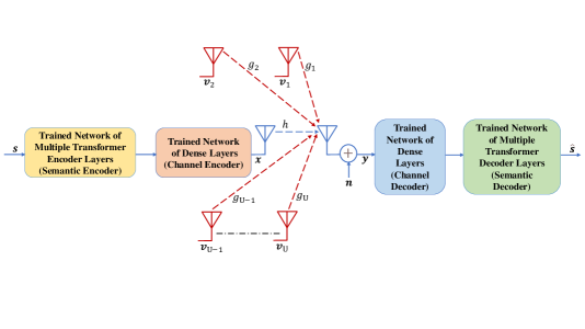
Figure 1: A trained DeepSC under RFI from single-antenna RFI emitters.

Following the lead of the works in [5, 29], let $\bm{s}\mathrel{\mathop{:}}=[w_{1},w_{2},\ldots,w_{L}]$ be a sentence of $L$ words – $w_{l}$ being the $l$-th word for all $l\in[L]$ – to be transmitted by the trained DeepSC transmitter shown in Fig. 1. As per Fig. 1 and with respect to (w.r.t.) an input $\bm{s}$, the trained semantic encoder network coupled with the trained channel encoder network will extract the semantic features from the input text and map them into semantic symbols (termed DeepSC symbols hereinafter) $\bm{x}$ that can be expressed (via [5, eq. (1)]) as

$$\bm{x}=C_{\hat{\bm{\alpha}}}(S_{\hat{\bm{\beta}}}(\bm{s}))\in\mathbb{C}^{1\times KL},$$ (2)

where $K$ is the average number of mapped semantic symbols per word in $\bm{s}$ [29], $S_{\hat{\bm{\beta}}}(\cdot)$ represents the trained semantic encoder network with a parameter set $\hat{\bm{\beta}}$, and $C_{\hat{\bm{\alpha}}}(\cdot)$ is the trained channel encoder network with a parameter set $\hat{\bm{\alpha}}$. We use these trained networks to realize – similar to the authors of [5] and without loss of generality – the transmission of $\bm{x}$ over an independent Rayleigh fading channel $h\sim\mathcal{CN}(0,1)$ via a wireless environment experiencing (MI) RFI from $U$ independent RFI emitters emitting RFI over an independent Rayleigh fading channel $g_{u}\sim\mathcal{CN}(0,1)$ for all $u\in[U]$. For this setting, the received DeepSC signal $\bm{y}$ is given by

$$\bm{y}=h\bm{x}+\textstyle\sum_{u=1}^{U}g_{u}\bm{v}_{u}+\bm{n}\in\mathbb{C}^{1\times KL},$$ (3)

where the elements of the DeepSC symbols are power-constrained w.r.t. the maximum transmission power $P_{\textnormal{max}}^{s}$ W as $\mathbb{E}\{[\textnormal{Re}\{(\bm{x})_{i}\}]^{2}\},\mathbb{E}\{[\textnormal{Im}\{(\bm{x})_{i}\}]^{2}\}\leq P_{\textnormal{max}}^{s}$ for all $i\in[KL]$; $\bm{v}_{u}\in\mathbb{C}^{1\times KL}$ is a row vector comprising the unknown transmitted RFI symbols of the $u$-th RFI emitter; the $u$-th RFI emitter is power-constrained w.r.t. its corresponding minimum RFI power $P_{\textnormal{min}}^{i,u}$ and maximum RFI power $P_{\textnormal{max}}^{i,u}$ as $P_{\textnormal{min}}^{i,u}\leq\mathbb{E}\{[\textnormal{Re}\{(\bm{v}_{u})_{i}\}]^{2}\},\mathbb{E}\{[\textnormal{Im}\{(\bm{v}_{u})_{i}\}]^{2}\}\leq P_{\textnormal{max}}^{i,u}$ for all $i\in[KL]$ and $u\in[U]$; and $\bm{n}\in\mathbb{C}^{1\times KL}$ is the additive white Gaussian noise (AWGN) characterized as $\bm{n}\sim\mathcal{CN}(\bm{0},\sigma^{2}\bm{I}_{KL})$. Meanwhile, the received DeepSC signal $\bm{y}\in\mathbb{C}^{1\times KL}$ goes through the trained channel decoder network and then the trained semantic decoder network – as in Fig. 1 – to generate the recovered sentence $\hat{\bm{s}}$ that equates (via [5, eq. (3)]) to

$$\hat{\bm{s}}=S_{\hat{\bm{\theta}}}(C_{\hat{\bm{\delta}}}(\bm{y})),$$ (4)

where $C_{\hat{\bm{\delta}}}(\cdot)$ denotes the trained channel decoder network with a parameter set $\hat{\bm{\delta}}$ and $S_{\hat{\bm{\theta}}}(\cdot)$ designates the trained semantic decoder network with a parameter set $\hat{\bm{\theta}}$.

We employ the aforementioned system setup – equating the transmitted sentence $\bm{s}$ and the recovered sentence $\hat{\bm{s}}$ via (2) and (4), respectively – and move on to our problem formulation.

II-B Problem Formulation

DeepSC’s performance can be assessed via semantic similarity between $\bm{s}$ $\&$ $\hat{\bm{s}}$ as [29, eq. (1)]

$$\eta(\bm{s},\hat{\bm{s}})\mathrel{\mathop{:}}=\frac{\bm{B}(\bm{s})\bm{B}(\hat{\bm{s}})^{T}}{\|\bm{B}(\bm{s})\|\|\bm{B}(\hat{\bm{s}})\|},$$ (5)

where $\eta(\bm{s},\hat{\bm{s}})$ quantifies the semantic similarity and $\bm{B}(\cdot)$ denotes the output of BERT (bidirectional encoder representations from transformers [30]) – a gigantic pre-trained model comprising billions of parameters that are used to mine semantic information [5]. The value of metric $\eta(\bm{s},\hat{\bm{s}})$ is between 0 and 1, implying semantic irrelevance and semantic consistency [31], respectively. Meanwhile, $\eta(\bm{s},\hat{\bm{s}})$ depends on the average number of semantic symbols per word $K$ and the signal-to-noise ratio (SNR) $\gamma$ [5]. Accordingly, $\eta(\bm{s},\hat{\bm{s}})$ can be expressed via the semantic similarity function $\varepsilon(K,\gamma)$ and, hence, we have [29]

$$\eta(\bm{s},\hat{\bm{s}})=\varepsilon(K,\gamma).$$ (6)

The authors of [29] overcame the analytical intractability of $\varepsilon(K,\gamma)$ by exploiting the generalized logistic function to approximate $\varepsilon(K,\gamma)$ for any given $K$ as [29, eq. (3)]

$$\varepsilon(K,\gamma)\approx\tilde{\varepsilon}_{K}(\gamma)=A_{K,1}+\frac{A_{K,2}-A_{K,1}}{1+e^{-(C_{K,1}\gamma+C_{K,2})}},$$ (7)

where $A_{K,1}>0$, $A_{K,2}>0$, and $C_{K,1}>0$ denote the lower (left) asymptote, the upper (right) asymptote, and the logistic growth rate, respectively; $C_{K,2}$ controls the logistic midpoint [29]. In light of (7), $0\leq\varepsilon(K,\gamma)\leq 1$, $\kappa\mathrel{\mathop{:}}=A_{K,1}/(A_{K,1}-A_{K,2})\geq 0$, and the generalized logistic function renders an accurate approximation for any $K$, as demonstrated in [29, Fig. 2]. Meanwhile, employing (7) in the right-hand side (RHS) of (6), the following highly-accurate approximation ensues:

$$\eta(\bm{s},\hat{\bm{s}})\approx A_{K,1}+\frac{A_{K,2}-A_{K,1}}{1+e^{-(C_{K,1}\gamma+C_{K,2})}}.$$ (8)

The asymptotic performance analysis of DeepSC is mathematically tractable via (8). Thus, (8) paves the way for deriving DeepSC’s performance limits.

To assess the performance of DeepSC using probability as a lens, we introduce a new semantic metric – named the upper tail probability of a semantic similarity – applicable for evaluating the asymptotic/non-asymptotic performance of text SemCom systems, as formalized in Definition 1.

Definition 1.

The upper tail probability of $\eta(\bm{s},\hat{\bm{s}})$ w.r.t. $\eta_{\textnormal{min}}\in[0,1]$ is computed as

$$p(\eta_{\textnormal{min}})\mathrel{\mathop{:}}=\mathbb{P}\big{(}\eta(\bm{s},\hat{\bm{s}})\geq\eta_{\textnormal{min}}\big{)},$$ (9)

where the metric $\eta(\bm{s},\hat{\bm{s}})$ is defined in (5) and $\eta_{\textnormal{min}}$ is the minimum semantic similarity.

Regarding (9), $p(0)\mathrel{\mathop{:}}=\mathbb{P}\big{(}\eta(\bm{s},\hat{\bm{s}})\geq 0\big{)}$ is a probabilistic metric that quantifies the probability of semantic similarity by any text SemCom technique being greater than or equal to 0. Using $p(0)$, therefore, we hereinafter formulate problems on the asymptotic performance analysis of DeepSC under single-interferer RFI – hereinafter termed RFI – and under MI RFI. We begin with the former.

II-B1 Problems on the Asymptotic Performance Analysis of DeepSC under RFI

to study the asymptotic performance of DeepSC under infinitesimally small RFI and a very low SNR, we formulate the following problem:

Problem 1.

Characterize $\displaystyle\lim_{\sigma^{2}\to\infty}p(0)$ and $\displaystyle\lim_{P_{\textnormal{max}}^{s}\to 0}p(0)$.

Solving Problem 1 will help us understand the asymptotic performance of DeepSC – w.r.t. infinitesimally small RFI – for very low SNR regimes. These are for a very large noise power and a very small maximum transmission power of the DeepSC symbols, as captured by Problem 1. On the other hand, to investigate the asymptotic performance of DeepSC under RFI and a very low signal-to-interference-plus-noise ratio (SINR), we formulate the underneath problem w.r.t. $P_{\textnormal{min}}^{i}\mathrel{\mathop{:}}=P_{\textnormal{min}}^{i,1}$.

Problem 2.

Derive $\displaystyle\lim_{P_{\textnormal{min}}^{i}\to\infty}p(0)$ and $\displaystyle\lim_{P_{\textnormal{max}}^{s}\to 0}p(0)$.

Solving Problem 2 will help us understand the asymptotic performance of DeepSC – under RFI – for very low SINR regimes. Such regimes can be for a very large power of the emitted RFI and a very small maximum transmission power of the DeepSC symbols, as captured by Problem 2. Next, we proceed to our third set of formulated problems.

II-B2 Problems on the Asymptotic Performance Analysis of DeepSC under MI RFI

to understand DeepSC’s asymptotic performance under MI RFI and a very low SINR, we formulate the ensuing problem for $U>1$ and $\tilde{P}_{\textnormal{min}}^{i}\mathrel{\mathop{:}}=\textnormal{min}\big{(}P_{\textnormal{min}}^{i,1},P_{\textnormal{min}}^{i,2},\ldots,P_{\textnormal{min}}^{i,U}\big{)}$.

Problem 3.

Derive $\displaystyle\lim_{P_{\textnormal{max}}^{s}\to 0}p(0)$, $\displaystyle\lim_{\tilde{P}_{\textnormal{min}}^{i}\to\infty}p(0)$, and $\displaystyle\lim_{U\to\infty}p(0)$.

Solving Problem 3 will help us understand the asymptotic performance of DeepSC – under MI RFI – for very low SINR regimes. Such regimes can be for a very small maximum transmission power of the DeepSC symbols, a large power of all RFI emitters, and an enormous number of RFI emitters, as captured by Problem 3. Apart from Problems 1-3,we also formulate the following novel problems.

II-B3 Problems on the Non-Asymptotic Performance Analysis of DeepSC under MI RFI

we follow up with Problems 4 and 5 on DeepSC’s non-asymptotic performance.

Problem 4.

For a given $\eta_{\textnormal{min}}\in[0,1]$, derive the practical limits of DeepSC w.r.t. $p(\eta_{\textnormal{min}})$.

Problem 5.

Derive the outage probability of DeepSC.

Problems 1-5 are novel problems considering the fact that the performance analysis of any SemCom system is fundamentally challenging – as outlined in Section I – and no work has provided an asymptotic/non-asymptotic performanceanalysis of any SemCom technique. Overcoming this limitation w.r.t. Problems 1-3, we hereunder present the asymptotic performance limits of DeepSC [5] under (MI) RFI.

III Performance Limits of DeepSC

We begin with DeepSC’s performance limits under RFI.

III-A Performance Limits of DeepSC Subjected to RFI

We use (8) and (9) w.r.t. the system model in Section II-A to derive the following theorem.

Theorem 1.

Per the approximation in (8) and Sec. II-A’s settings, DeepSC manifests the following performance limits – for a given $K$ – under infinitesimally small RFI: $i)\lim_{\sigma^{2}\to\infty}p(0)=0$; $ii)\lim_{P_{\textnormal{max}}^{s}\to 0}p(0)=0$, where these results are valid w.r.t. $\alpha\leq\kappa\leq 1$ given $\alpha\mathrel{\mathop{:}}=e^{C_{K,2}}/(1+e^{C_{K,2}})$ and $\kappa\mathrel{\mathop{:}}=A_{K,1}/(A_{K,1}-A_{K,2})$.

Proof.

The proof is in Appendix A.

Per Theorem 1, $\lim_{\sigma^{2}\to\infty}p(0)=0$ and $\lim_{P_{\textnormal{max}}^{s}\to 0}p(0)=0$corroborate – whenever $\sigma^{2}\to\infty$ and $P_{\textnormal{max}}^{s}\to 0$ – that $\eta(\bm{s},\hat{\bm{s}})=0$, which affirms maximum semantic dissimilarity (or semantic irrelevance) [31]. Consequently, Theorem 1 translates to the following remarks.

Remark 1.

DeepSC – per Sec. II-A’s settings – exhibits the following performance limits when it is subjected to infinitesimally small RFI: $i)$ DeepSC will generate semantically irrelevant sentences as the noise power gets large; $ii)$ DeepSC will generate semantically irrelevant sentences as the DeepSC symbols’ maximum transmission power tends to zero Watt (W).

Remark 2.

Contrary to the analytically unsubstantiated sentiment that SemCom techniques (such as DeepSC) work well in very low SNR regimes while outperforming the techniques of conventional communication systems, Theorem 1 asserts that DeepSC will generate semantically irrelevant sentences as the noise power gets large and the DeepSC symbols’ maximum transmission power approaches zero W.

Similarly, the impact of moderate/strong RFI on DeepSC’s performance is quantified below.

Theorem 2.

According to Sec. II-A’s settings and the approximation in (8), DeepSC manifests the following performance limits – for a given $K$ – under RFI: $i)\lim_{P_{\textnormal{min}}^{i}\to\infty}p(0)=0$; $ii)\lim_{P_{\textnormal{max}}^{s}\to 0}p(0)=0$, where these results are true w.r.t. $\alpha\leq\kappa\leq 1$.

Proof.

The proof is in Appendix B.

Theorem 2 asserts the following foundational insight.

Remark 3.

DeepSC – per Sec. II-A’s settings – displays the following performance limits when it is subjected to RFI: $i)$ DeepSC will recover semantically irrelevant sentences as the DeepSC symbols’ maximum transmission power nears zero W; $ii)$ DeepSC will produce semantically irrelevant sentences as the power emitted by RFI becomes large, which attests to the fact that strong RFI can destroy the faithfulness of SemCom by producing a huge amount of semantic noise.

Strong RFI emitter indeed create significant semantic noise, which can affect the reliability of SemCom that can be decimated by MI RFI (due to several RFI emitters). Therefore, we henceforth expose the performance limits of DeepSC subjected to MI RFI.

III-B Performance Limits of DeepSC Subjected to MI RFI

Considering MI RFI modeled as in Sec. II-A, the approximation in (8), and (9), we derive the performance limits of DeepSC, as formalized in the following theorem.

Theorem 3.

Pursuant to Sec. II-A’s settings and the approximation in (8), DeepSC exhibits the following performance limits – for a given $K$ – under MI RFI: $i)\lim_{P_{\textnormal{max}}^{s}\to 0}p(0)=0$; $ii)\lim_{\tilde{P}_{\textnormal{min}}^{i}\to\infty}p(0)=0$; $iii)\lim_{U\to\infty}p(0)=0$, where these results are valid w.r.t. $\alpha\leq\kappa\leq 1$, $U>1$, and $P_{\textnormal{max}}^{s}\leq\beta(U-1)\tilde{P}_{\textnormal{min}}^{i}$ such that $\beta=\ln\big{[}\kappa/(1-\kappa)\big{]}/C_{K,1}-C_{K,2}/C_{K,1}$.

Proof.

The proof is in Appendix C.

The following intuitive remark stems from Theorem 3.

Remark 4.

DeepSC – per Sec. II-A’s settings – manifests the following performance limits when it is subjected to MI RFI (from $U\geq 2$ RFI emitters): $i)$ DeepSC will generate semantically irrelevant sentences as the DeepSC symbols’ maximum transmission power tends to zero W; $ii)$ DeepSC will produce semantically irrelevant sentences as all RFI emitters get strong; $iii)$ DeepSC will produce semantically irrelevant sentences as the number of RFI emitters becomes enormous (i.e., $U\to\infty$).

Summarizing, the following remarks ensue.

Remark 5.

Although the performance analyses (Appendices A-C) that led to the performance limits per Theorems 1-3 are regarding DeepSC, the introduced probabilistic framework – with the proposed semantic metric – is particularly applicable to many text SemCom techniques and generally relevant in speech SemCom, image SemCom, and video SemCom.

Remark 6.

In view of a wireless attack with RFI that changes the semantics of information transmitted using SemCom [20], Theorems 2 and 3 underscore DeepSC’s security vulnerability.

Aside from Theorems 1-3, DeepSC’s practical limits and outage probability provide useful insights, as detailed below.

IV The Practical Limits and Outage Probability of DeepSC

IV-A The Practical Limits of DeepSC

In the practical design of DeepSC, $\eta_{\textnormal{min}}\geq 0.8$ can be a desirable range. To this end, understanding the practical limits of DeepSC for a given $\eta_{\textnormal{min}}$ and $K$ is crucial. For this purpose, we derive DeepSC’s practical limits, as formalized below.

Corollary 1.

Per Sec. II-A’s settings and the approximation in (8), DeepSC manifests the following performance limits – for a given $\eta_{\textnormal{min}}$ and $K$ – under MI RFI: $p(\eta_{\textnormal{min}})\leq P_{\textnormal{max}}^{s}/[\beta_{K}(\eta_{\textnormal{min}})(U-1)\tilde{P}_{\textnormal{min}}^{i}]$, where this is valid w.r.t. $P_{\textnormal{max}}^{s}\leq\beta_{K}(\eta_{\textnormal{min}})(U-1)\tilde{P}_{\textnormal{min}}^{i}$ such that $\beta_{K}(\eta_{\textnormal{min}})\mathrel{\mathop{:}}=\ln[\kappa_{K}(\eta_{\textnormal{min}})/(1-\kappa_{K}(\eta_{\textnormal{min}}))]/C_{K,1}-C_{K,2}/C_{K,1}$ and $\alpha<\kappa_{K}(\eta_{\textnormal{min}})\leq 1$ given $\kappa_{K}(\eta_{\textnormal{min}})\mathrel{\mathop{:}}=(\eta_{\textnormal{min}}-A_{K,1})/(A_{K,2}-A_{K,1})$.

Proof.

The proof is in Appendix D.

This result helps to bound the outage probability of DeepSC.

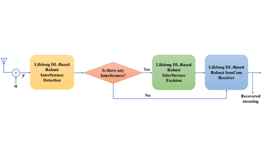
Figure 2: A (generic) lifelong DL-based IR² SemCom system.

IV-B The Outage Probability of DeepSC

Adopting a popular performance metric of wireless communication [33], DeepSC’s outage probability is defined as

$$P_{\textnormal{out}}(\eta_{\textnormal{min}})\mathrel{\mathop{:}}=\mathbb{P}\big{(}\eta(\bm{s},\hat{\bm{s}})<\eta_{\textnormal{min}}\big{)}\stackrel{{\scriptstyle(a)}}{{=}}1-p(\eta_{\textnormal{min}}),$$ (10)

where $(a)$ is due to (9) and (10) leads to the following lemma.

Lemma 1.

Per Sec. II-A’s settings and the approximation in (8), the outage probability of DeepSC – for a given $\eta_{\textnormal{min}}$ and $K$ – under MI RFI satisfies the bound: $P_{\textnormal{out}}(\eta_{\textnormal{min}})\geq 1-P_{\textnormal{max}}^{s}/[\beta_{K}(\eta_{\textnormal{min}})(U-1)\tilde{P}_{\textnormal{min}}^{i}]$, where this is valid w.r.t.$\alpha<\kappa_{K}(\eta_{\textnormal{min}})\leq 1$ and $P_{\textnormal{max}}^{s}\leq\beta_{K}(\eta_{\textnormal{min}})(U-1)\tilde{P}_{\textnormal{min}}^{i}$.

Proof.

The bound follows from (10) and Corollary 1. ∎

Deploying Lemma 1, the underneath optimization ensues.

IV-C Optimization Based On the Outage Probability of DeepSC

According to (10), the $K$ that minimizes $P_{\textnormal{out}}(\eta_{\textnormal{min}})$ is the one that maximizes $p(\eta_{\textnormal{min}})$ given $K\in\{1,2,\ldots,K_{\textnormal{max}}\}$. Thus, the following optimization problem ensues:

$$\operatorname*{arg\,max}_{K}\quad p(\eta_{\textnormal{min}})\hskip 8.53581pt\textnormal{s.t.}\hskip 8.53581pt0\leq\eta_{\textnormal{min}}\leq 1;\hskip 5.69054ptK\leq K_{\textnormal{max}}.$$ (11)

Consequently, the underneath lemma follows.

Lemma 2.

The solution of (11) is $K^{\star}=K_{\textnormal{max}}$.

Proof.

Using Corollary 1, (11) can also be cast as

$$\operatorname*{arg\,max}_{K}\quad P_{\textnormal{max}}^{s}/[\beta_{K}(\eta_{\textnormal{min}})(U-1)\tilde{P}_{\textnormal{min}}^{i}]$$ (12a)

s.t. $$0\leq\eta_{\textnormal{min}}\leq 1;\hskip 5.69054ptK\leq K_{\textnormal{max}}.$$ (12b)

Discarding constants from the optimization objective in (12a) produces an equivalent optimization problem given by

$$\operatorname*{arg\,min}_{K}\quad\beta_{K}(\eta_{\textnormal{min}})\hskip 8.53581pt\textnormal{s.t.}\hskip 8.53581pt0\leq\eta_{\textnormal{min}}\leq 1;\hskip 5.69054ptK\leq K_{\textnormal{max}}.$$ (13)

As it can be seen in [29, Fig. 2], $\tilde{\varepsilon}_{K}(\gamma)\geq\tilde{\varepsilon}_{\tilde{K}}(\gamma)$ for any $\gamma$ and $K>\tilde{K}$. For any $K>\tilde{K}$ and $\gamma$, thus, $\mathbb{P}(\tilde{\varepsilon}_{K}(\gamma)\geq\eta_{\textnormal{min}})\geq\mathbb{P}(\tilde{\varepsilon}_{\tilde{K}}(\gamma)\geq\eta_{\textnormal{min}})$, and it follows from (70)-(71g) that

$$\mathbb{P}\big{(}\gamma\geq\beta_{K}(\eta_{\textnormal{min}})\big{)}\geq\mathbb{P}\big{(}\gamma\geq\beta_{\tilde{K}}(\eta_{\textnormal{min}})\big{)},$$ (14)

where $\beta_{\tilde{K}}(\eta_{\textnormal{min}})=\beta_{K}(\eta_{\textnormal{min}})\big{|}_{K=\tilde{K}}$. Hence, it follows from (14) that $\beta_{K}(\eta_{\textnormal{min}})\leq\beta_{\tilde{K}}(\eta_{\textnormal{min}})$ w.r.t. all $K>\tilde{K}$ and hence $\beta_{K_{\textnormal{max}}}(\eta_{\textnormal{min}})\leq\beta_{K_{\textnormal{max}}-1}(\eta_{\textnormal{min}})\leq\ldots\leq\beta_{K}(\eta_{\textnormal{min}})\leq\ldots\leq\beta_{1}(\eta_{\textnormal{min}})$. Using this relation in (13), the optimal $K$ that minimizes the outage probability of DeepSC is $K^{\star}=K_{\textnormal{max}}$. This ends the proof of Lemma 2.∎

Remark 7.

The optimal $K$ that minimizes the outage probability of DeepSC subjected to MI RFI is $K_{\textnormal{max}}$.

V Toward IR² 6G Wireless Systems

In radio frequency (RF) operating systems such as radio astronomy, microwave radiometry, and satellite communication, RFI causes performance loss for orbital and terrestrial interferers, malicious interferers, spoofing attacks, and RF jammers [23]. RFI also impacts wireless systems based on ultra-wideband communication, radars, and cognitive radios due to wideband interferers, wideband jammers, and imperfect spectrum sensing, respectively [23]. By the same token, interference is also a big concern for medical devices such as medical implants [34], public safety networks [35], wireless body area networks [35], and critical infrastructure such as Smart Grid, smart manufacturing, and the healthcare industry [35].These use cases of interference and RFI in the aforementioned contemporary wireless systems underscore the need for IR² wireless systems in 6G and beyond. For 6G and beyond, on the other hand, SemCom holds promise in minimizing bandwidth consumption, power usage, and transmission delay. Accordingly, there is a need for IR² SemCom systems as such systems are also impacted by RFI, in particular, and interference, in general.

Inspired by the traditional interference-resistant wireless communication advocated in [23] and state-of-the-art advancements in lifelong DL [36, 37, 38], we propose a generic lifelong DL-based IR² SemCom system schematized in Fig. 2. As seen in Fig. 2, the lifelong DL-based robust interference detection module learns the presence of interference in real-time – regardless of its type – by learning multiple distributions of interference on a continual basis. If this module flags the presence of interference, the lifelong DL-based robust interference excision module excises the received interference in real-time – irrespective of its angle of arrival (AoA) – while learning the AoA of interference in a lifelong manner. The output of this module is then fed to the lifelong DL-based robust SemCom receiver, which is designed to accurately recover the meaning of the transmitted message.

To gain insight into the performance of a lifelong DL-based IR² DeepSC per Fig. 2, let $\breve{p}(\eta_{\textnormal{min}})\mathrel{\mathop{:}}=\mathbb{P}(\varepsilon(K,\breve{\gamma})\geq\eta_{\textnormal{min}})$ be its exhibited SemCom performance given that $\breve{\gamma}$ is the SINR after applying a lifelong DL-based robust interference excision. Suppose the optimal lifelong DL network at the $t$-th deployment instant for a robust interference excision is $\bm{\Phi}_{t}^{\star}(\cdot)$. Hence, the signal output after a robust interference excision is $\bm{\Phi}_{t}^{\star}(\bm{y})$. For $\bm{y}$ defined in (3), let us presume that $\bm{\Phi}_{t}^{\star}(h\bm{x}+\textstyle\sum_{u=1}^{U}g_{u}\bm{v}_{u}+\bm{n})\approx\bm{\Phi}_{t,1}^{\star}(h\bm{x})+\bm{\Phi}_{t,2}^{\star}(\textstyle\sum_{u=1}^{U}g_{u}\bm{v}_{u})+\bm{\Phi}_{t,3}^{\star}(\bm{n})$ for $\big{\{}\bm{\Phi}_{t,j}^{\star}(\cdot)\big{\}}_{j=1}^{3}$ being the respective lifelong DL networks for the received signal, impinging RFI, and noise during the $t$-th deployment instant. W.r.t. this approximation, the underneath corollary asserts the performance gain of the lifelong DL-basedIR² DeepSC over DeepSC under large $U$.

Corollary 2.

Assume a lifelong DL-based IR² DeepSC per Fig. 2 that is equipped with a perfect interference detector.If $\bm{\Phi}_{t,2}^{\star}(\textstyle\sum_{u=1}^{U}g_{u}\bm{v}_{u})\approx\bm{0}$ for all $t\in\mathbb{N}$ and $0<(\bm{\Phi}_{t,1}^{\star}(h\bm{x}))_{i},(\bm{\Phi}_{t,3}^{\star}(\bm{n}))_{i}<\infty$ for all $t\in\mathbb{N}$ and $i\in[KL]$, the following are true with a high probability:

• $\displaystyle\lim_{U\to\infty}\breve{p}(\eta_{\textnormal{min}})>>\displaystyle\lim_{U\to\infty}p(\eta_{\textnormal{min}})$ for high SNR regimes;

• $\displaystyle\lim_{U\to\infty}\breve{p}(\eta_{\textnormal{min}})\geq\displaystyle\lim_{U\to\infty}p(\eta_{\textnormal{min}})$ for low SNR regimes.

Proof.

The proof is in Appendix E.

We continue to simulation and computer experiment results.

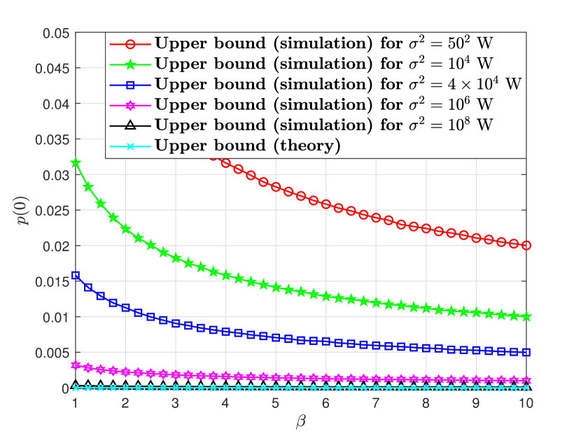
Figure 3: $p(0)$ versus $\beta$ under infinitesimally small RFI, fixed $P_{\textnormal{max}}^{s}=5$ W, and varying $\sigma^{2}$: $N=10^{7}$.

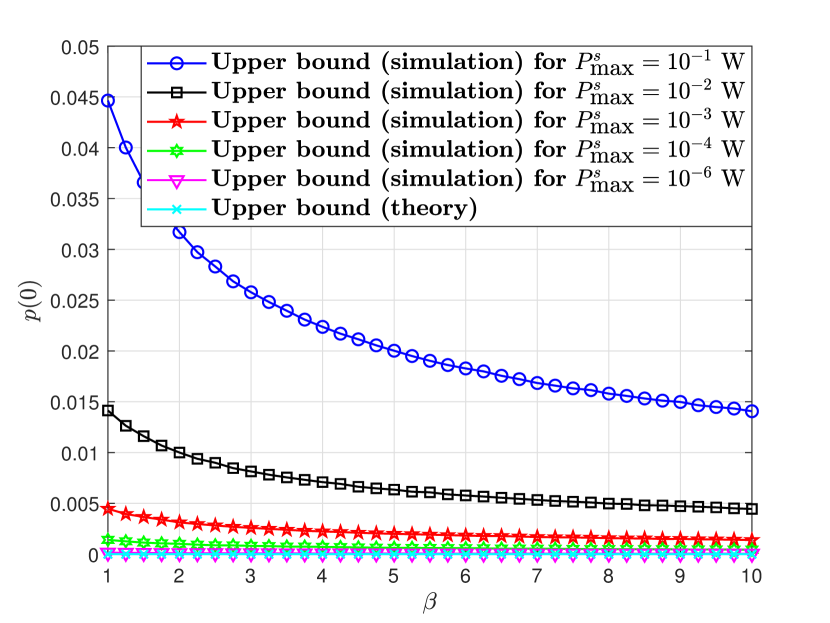
Figure 4: $p(0)$ versus $\beta$ under infinitesimally small RFI, fixed $\sigma^{2}=100$ W, and varying $P_{\textnormal{max}}^{s}$: $N=10^{7}$.

VI Simulation and Computer Experiment Results

The results of the simulations validating Theorems 1, 2, and 3 are presented in this section. Specifically, this section presents simulation results pertaining to Monte Carlo simulations with infinitesimally small RFI, RFI, and MI RFI. This section also presents computer experiment results that substantiate our theory. We begin with the results of the simulations with infinitesimally small RFI.

VI-A Simulation Results with Infinitesimally Small RFI

W.r.t. the infinitesimally small RFI examined in Theorem 1,it follows from Appendix A, (16g), and (20b) that $p(0)\leq\mathbb{P}\Big{(}\frac{2P_{\textnormal{max}}^{s}}{\sigma^{2}}\frac{\big{(}[\sqrt{2}\textnormal{Re}\{h\}]^{2}+[\sqrt{2}\textnormal{Im}\{h\}]^{2}\big{)}}{[\sqrt{2}/\sigma\textnormal{Re}\{(\bm{n})_{i}\}]^{2}}\geq\beta\Big{)}$, where $\beta\in\mathbb{R}^{+}$ is a constant per (17) and $\sqrt{2}\textnormal{Re}\{h\},\sqrt{2}\textnormal{Im}\{h\},\sqrt{2}/\sigma\textnormal{Re}\{(\bm{n})_{i}\}\sim\mathcal{N}(0,1)$ are independent standard normal RVs. For these RVs, if we consider $N$ realizations of the Rayleigh fading channel $h$ and the AWGN $(\bm{n})_{i}$, the upper bound of $p(0)$ can be computed numerically as $p(0)\leq\frac{1}{N}\sum_{k=1}^{N}\mathbb{I}\Big{\{}\frac{2P_{\textnormal{max}}^{s}}{\sigma^{2}}\frac{\big{(}X_{k}^{2}+Y_{k}^{2}\big{)}}{Z_{k}^{2}}\geq\beta\Big{\}}$, where $X_{k}\mathrel{\mathop{:}}=\sqrt{2}\textnormal{Re}\{h_{k}\},Y_{k}\mathrel{\mathop{:}}=\sqrt{2}\textnormal{Im}\{h_{k}\}\sim\mathcal{N}(0,1)$ are independent standard normal RVs regarding the $k$-th realization of the Rayleigh fading channel $h$ and, $Z_{k}\mathrel{\mathop{:}}=\sqrt{2}/\sigma\textnormal{Re}\{(\bm{n})_{i,k}\}\sim\mathcal{N}(0,1)$ denotes an independent standard normal RV for the $k$-th realization of the AWGN $(\bm{n})_{i}$. Accordingly, we carry out Monte Carlo simulations in MATLAB^® by generating the $3N$ independent standard normal RVs $\big{\{}X_{k}\big{\}}_{k=1}^{N}$, $\big{\{}Y_{k}\big{\}}_{k=1}^{N}$, and $\big{\{}Z_{k}\big{\}}_{k=1}^{N}$ to compute the upper bound in the RHS of the above numerical expression by $1)$ fixing $P_{\textnormal{max}}^{s}$ and varying $\sigma^{2}$ and $2)$ fixing $\sigma^{2}$ and varying $P_{\textnormal{max}}^{s}$. For these settings, the produced $p(0)$ versus $\beta$ plots are presented in Figs. 4 and 4.

Fig. 4 demonstrates that $p(0)$ approaches zero as $\sigma^{2}$ gets large – regardless of $\beta$ – and hence $\displaystyle\lim_{\sigma^{2}\to\infty}p(0)=0$. This validates the first part of Theorem 1. Similarly, Fig. 4 shows that $p(0)$ tends to zero as $P_{\textnormal{max}}^{s}$ gets infinitesimally small – irrespective of $\beta$ – and hence $\displaystyle\lim_{P_{\textnormal{max}}^{s}\to 0}p(0)=0$. This verifies the second part of Theorem 1. Thus, Theorem 1 is now substantiated. Next, we present the results of Monte Carlo simulations with RFI.

VI-B Simulation Results with RFI

In reference to the RFI addressed in Theorem 2, it follows from Appendix B, (41), and (44b) that $p(0)\leq\mathbb{P}\Big{(}\frac{P_{\textnormal{max}}^{s}\big{(}[\sqrt{2}\textnormal{Re}\{h\}]^{2}+[\sqrt{2}\textnormal{Im}\{h\}]^{2}\big{)}}{P_{\textnormal{min}}^{i}[\sqrt{2}\textnormal{Re}\{g\}]^{2}}\geq\beta\Big{)}$, where $\beta\geq 0$ is a constant defined in (17) and $\sqrt{2}\textnormal{Re}\{h\},\sqrt{2}\textnormal{Im}\{h\},\sqrt{2}\textnormal{Re}\{g\}\sim\mathcal{N}(0,1)$ are independent standard normal RVs. For these RVs, if we consider $N$ realizations of the independent Rayleigh fading channels $\{h,g\}$, the upper bound of $p(0)$ can be obtained numerically as $p(0)\leq\frac{1}{N}\sum_{k=1}^{N}\mathbb{I}\Big{\{}\frac{P_{\textnormal{max}}^{s}}{P_{\textnormal{min}}^{i}}\frac{\big{(}A_{k}^{2}+B_{k}^{2}\big{)}}{C_{k}^{2}}\geq\beta\Big{\}}$, where $A_{k}\mathrel{\mathop{:}}=\sqrt{2}\textnormal{Re}\{h_{k}\},B_{k}\mathrel{\mathop{:}}=\sqrt{2}\textnormal{Im}\{h_{k}\},C_{k}\mathrel{\mathop{:}}=\sqrt{2}\textnormal{Re}\{g_{k}\}\sim\mathcal{N}(0,1)$ are independent standard normal RVs for the $k$-th realization of the independent Rayleigh fading channels $\{h,g\}$. Consequently, we conduct Monte Carlo simulations in MATLAB^® by generating the $3N$ independent standard normal RVs $\big{\{}A_{k}\big{\}}_{k=1}^{N}$, $\big{\{}B_{k}\big{\}}_{k=1}^{N}$, and $\big{\{}C_{k}\big{\}}_{k=1}^{N}$ to calculate the upper bound in the RHS of the above numerical expression by $1)$ fixing $P_{\textnormal{max}}^{s}$ and varying $P_{\textnormal{min}}^{i}$ and $2)$ fixing $P_{\textnormal{min}}^{i}$ and varying $P_{\textnormal{max}}^{s}$. For these settings, the $p(0)$ versus $\beta$ plots are depicted in Figs. 6 and 6.

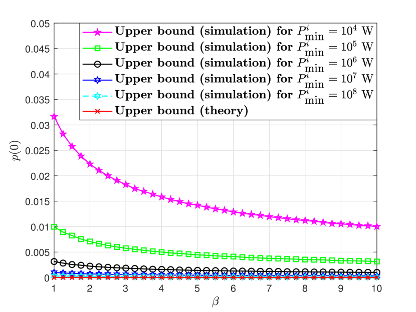
Figure 5: $p(0)$ versus $\beta$ under an RFI, fixed $P_{\textnormal{max}}^{s}=10$ W, and varying $P_{\textnormal{min}}^{i}$: $N=10^{7}$.

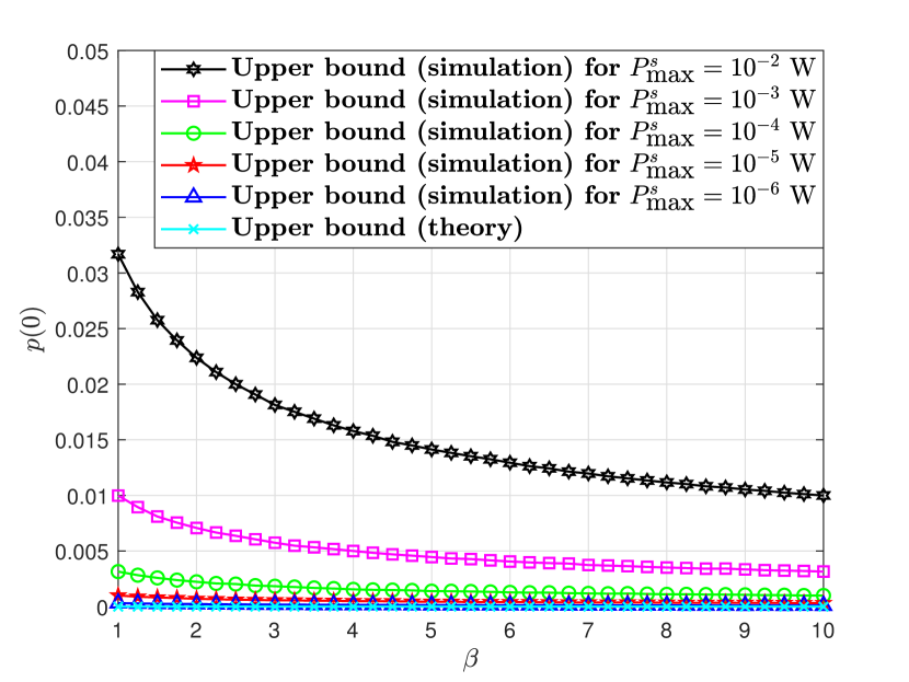
Figure 6: $p(0)$ versus $\beta$ under an RFI, fixed $P_{\textnormal{min}}^{i}=10$ W, and varying $P_{\textnormal{max}}^{s}$: $N=10^{7}$.

Fig. 6 shows that $p(0)$ approaches zero as $P_{\textnormal{min}}^{i}$ gets huge – irrespective of $\beta$ – and thus $\displaystyle\lim_{P_{\textnormal{min}}^{i}\to\infty}p(0)=0$. This validates the first part of Theorem 2. Similarly, Fig. 6 demonstrates that $p(0)$ gets close to zero as $P_{\textnormal{max}}^{s}$ becomes infinitesimally small – regardless of $\beta$ – and thus $\displaystyle\lim_{P_{\textnormal{max}}^{s}\to 0}p(0)=0$. This corroborates the second part of Theorem 2. Hence, Theorem 2is now confirmed. In the following, we present the results of the Monte Carlo simulations with MI RFI.

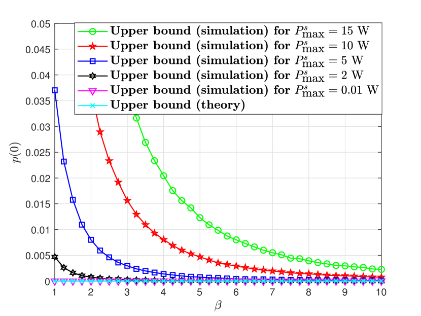
Figure 7: $p(0)$ versus $\beta$ under MI RFI, fixed $\tilde{P}_{\textnormal{min}}^{i}=10$ W, fixed $U=3$, and varying $P_{\textnormal{max}}^{s}$: $N=10^{6}$.

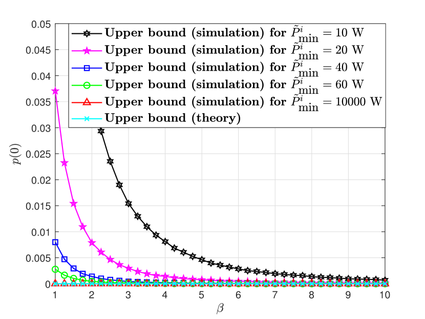
Figure 8: $p(0)$ versus $\beta$ under MI RFI, fixed $P_{\textnormal{max}}^{s}=10$ W, fixed $U=3$, and varying $\tilde{P}_{\textnormal{min}}^{i}$: $N=10^{6}$.

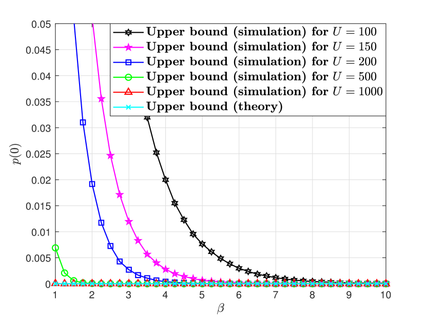
Figure 9: $p(0)$ versus $\beta$ under MI RFI, fixed $\tilde{P}_{\textnormal{min}}^{i}=0.1$ W, fixed $P_{\textnormal{max}}^{s}=10$ W, and varying $U$: $N=10^{6}$.

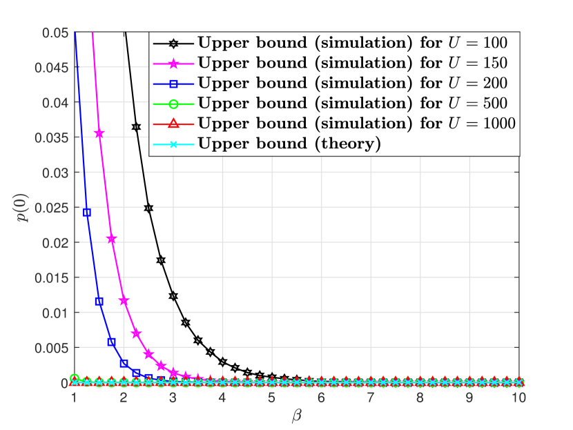
Figure 10: $p(0)$ versus $\beta$ under MI RFI, fixed $\tilde{P}_{\textnormal{min}}^{i}=0.15$ W, fixed $P_{\textnormal{max}}^{s}=10$ W, and varying $U$: $N=10^{6}$.

VI-C Simulation Results with MI RFI

Regarding the MI RFI considered in Theorem 3, it follows from Appendix C, (58), and (62a) that $p(0)\leq\mathbb{P}\Big{(}\frac{P_{\textnormal{max}}^{s}\big{(}[\sqrt{2}\textnormal{Re}\{h\}]^{2}+[\sqrt{2}\textnormal{Im}\{h\}]^{2}\big{)}}{\tilde{P}_{\textnormal{min}}^{i}\big{(}\sum_{u=1}^{U}[\sqrt{2}\textnormal{Re}\{g_{u}\}]^{2}+[\sqrt{2}\textnormal{Im}\{g_{u}\}]^{2}\big{)}}\geq\beta\Big{)}$, where $\beta\geq 0$ is a constant defined in (17); $\sqrt{2}\textnormal{Re}\{h\},\sqrt{2}\textnormal{Im}\{h\}\sim\mathcal{N}(0,1)$ are mutually independent standard normal RVs; and $\sqrt{2}\textnormal{Re}\{g_{u}\},\sqrt{2}\textnormal{Im}\{g_{u}\}\sim\mathcal{N}(0,1)$ (for all $u\in[U]$) are mutually independent standard normal RVs. For these RVs, if we consider $N$ realizations of the independent Rayleigh fading channels $\{h,g_{1},g_{2},\ldots,g_{U}\}$, the upper bound of $p(0)$ can be computed numerically as $p(0)\leq\frac{1}{N}\sum_{k=1}^{N}\mathbb{I}\Big{\{}\frac{P_{\textnormal{max}}^{s}}{\tilde{P}_{\textnormal{min}}^{i}}\frac{\big{(}D_{k}^{2}+E_{k}^{2}\big{)}}{\sum_{u=1}^{U}\big{(}F_{u,k}^{2}+G_{u,k}^{2}\big{)}}\geq\beta\Big{\}}$, where the RVs $D_{k}\mathrel{\mathop{:}}=\sqrt{2}\textnormal{Re}\{h_{k}\},E_{k}\mathrel{\mathop{:}}=\sqrt{2}\textnormal{Im}\{h_{k}\},F_{u,k}\mathrel{\mathop{:}}=\sqrt{2}\textnormal{Re}\{g_{u,k}\},G_{u,k}\mathrel{\mathop{:}}=\sqrt{2}\textnormal{Im}\{g_{u,k}\}\sim\mathcal{N}(0,1)$ are independent standard normal RVs for the $k$-th realization of the independent Rayleigh fading channels $\{h,g_{1},\ldots,g_{U}\}$. Accordingly, we perform Monte Carlo simulations in MATLAB^® by generating the $2N$ independent standard normal RVs $\big{\{}D_{k},E_{k}\big{\}}_{k=1}^{N}$ and the $2NU$ independent standard normal RVs $\big{\{}\big{\{}F_{u,k},G_{u,k}\big{\}}_{u=1}^{U}\big{\}}_{k=1}^{N}$ to determine the upper bound in the RHS of the above numerical expression by $1)$ fixing $\big{\{}\tilde{P}_{\textnormal{min}}^{i},U\big{\}}$ and varying $P_{\textnormal{max}}^{s}$; $2)$ fixing $\big{\{}P_{\textnormal{max}}^{s},U\big{\}}$ and varying $\tilde{P}_{\textnormal{min}}^{i}$; and $3)$ fixing $\big{\{}\tilde{P}_{\textnormal{min}}^{i},P_{\textnormal{max}}^{s}\big{\}}$ and varying $U$. For these settings, the $p(0)$ versus $\beta$ plots are shown in Figs. 8, 8, 10, and 10.

Fig. 8 demonstrates that $p(0)$ approaches zero as $P_{\textnormal{max}}^{s}$ gets infinitesimally small – regardless of $\beta$ – and hence $\displaystyle\lim_{P_{\textnormal{max}}^{s}\to 0}p(0)=0$. This validates the first part of Theorem 3. Similarly, Fig. 8 shows that $p(0)$ tends to zero as $\tilde{P}_{\textnormal{min}}^{i}$ gets gigantic – irrespective of $\beta$ – and thus $\displaystyle\lim_{\tilde{P}_{\textnormal{min}}^{i}\to\infty}p(0)=0$. This validates the second part of Theorem 3. Furthermore, Figs. 10 and 10 corroborate that $p(0)$ gets close to zero as $U$ (the number of RFI emitters) gets enormous – regardless of the minimum MI RFI power constraint and $\beta$ – and hence $\displaystyle\lim_{U\to\infty}p(0)=0$. This verifies the third part of Theorem 3,which is now corroborated. Meanwhile, we continue with simulation results regarding DeepSC’s practical limits.

VI-D Simulation Results Regarding DeepSC’s Practical Limits

Per Appendix C, the SINR under MI RFI at the $m$-th realization is $\gamma_{m}\mathrel{\mathop{:}}=\frac{|h_{m}|^{2}|(\bm{x})_{i}|^{2}}{\sum_{u=1}^{U}|g_{u,m}|^{2}|(\bm{v}_{u})_{i}|^{2}+|(\bm{n})_{m}|^{2}}$, where $h_{m},g_{m}\sim\mathcal{CN}(0,1)$. Without loss of generality and per the constraints of Corollary 1, we consider $|(\bm{x})_{i}|^{2}=|(\bm{v}_{u})_{i}|^{2}=1$ and $(\bm{n})_{m}\sim\mathcal{CN}(0,1)$, $P_{\textnormal{max}}^{s}=1.5$ W, $\tilde{P}_{\textnormal{min}}^{i}\in\{0.8,1\}$ W, and $U\in\{25,50,100\}$. Per this setting, the Monte Carlo simulation of DeepSC’s (approximated) performance is empirically evaluated as $p(\eta_{\textnormal{min}})=\frac{1}{N}\sum_{m=1}^{N}\mathbb{I}\big{\{}\gamma_{m}\geq\beta_{K}(\eta_{\textnormal{min}})\big{\}}$ while considering $N=10^{6}$. This leads to the $p(\eta_{\textnormal{min}})$ versus $\beta_{K}(\eta_{\textnormal{min}})$ plots depicted in Figs. 12 and 12. As it can be observed from these plots, the derived upper bound –formalized by Corollary 1 – gets very close to the simulation results as $\beta_{K}(\eta_{\textnormal{min}})$ gets bigger and $U$ gets larger.

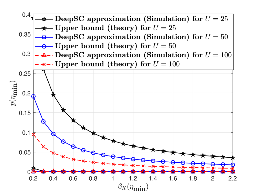
Figure 11: $p(\eta_{\textnormal{min}})$ versus $\beta_{K}(\eta_{\textnormal{min}})$ under $(\tilde{P}_{\textnormal{min}}^{i},P_{\textnormal{max}}^{s})=(0.8,1.5)$ W and $U\in\{25,50,100\}$: $N=10^{6}$.

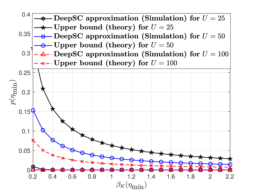
Figure 12: $p(\eta_{\textnormal{min}})$ versus $\beta_{K}(\eta_{\textnormal{min}})$ under $(\tilde{P}_{\textnormal{min}}^{i},P_{\textnormal{max}}^{s})=(1,1.5)$ W and $U\in\{25,50,100\}$: $N=10^{6}$.

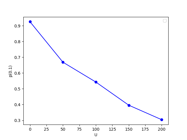
Figure 13: $p(0.1)$ versus $U$ exhibited by our trained DeepSC.

We now proceed to our computer experiment result.

VI-E Computer Experiment Result

We carried out extensive computer experiments on the training of DeepSC and its testing without and with MI RFI using a standard dataset named the proceedings of the European Parliament (Europarl). Employing 1.5 million training sentences and 300,000 validation sentences that were tokenized and vectorized from Europarl, we trained the DeepSC architecture [5] with Adam in Keras 2.9 with TensorFlow 2.9as a backend. We then tested our trained DeepSC model without and with time-varying Gaussian MI RFI [39, 40] by deploying 10,000 testing sentences that were also tokenized and vectorized from Europarl. This led to the $p(0.1)$ versus $U$plot that is depicted in Fig. 13. As seen in Fig. 13, DeepSC tends to produce semantically irrelevant sentences as the number of Gaussian RFI emitters becomes huge. This is what has been predicted by our developed theory. Consequently, we move on to our conclusion.

VII Concluding Summary and Research Outlook

As a potential enabler of 6G, SemCom is promising when it comes to minimizing power usage, bandwidth consumption, and transmission delay by minimizing the transmission of semantically irrelevant information. However, the fidelity of text, image, audio, and video SemCom techniques can be destroyed by a considerable semantic noise caused by RFI. Quantifying RFI’s impact while introducing a principled probabilistic framework applicable primarily for SemCom, we characterized the asymptotic performance limits, practical limits, and outage probability of DeepSC subjected to RFI and MI RFI. These derived performance limits of DeepSC were validated by extensive Monte Carlo simulations and computer experiments. The derived and validated asymptotic performance limits assert that strong RFI can destroy the faithfulness of SemCom by producing substantial semantic noise. Toward 6G and beyond, thus, there is a need for an adversarial electronic warfare-resistant SemCom system. To this end, this paper also proposed a generic lifelong DL-based IR² SemCom system.

As promising research outlook, this paper stimulates multiple lines of research on the design, analysis, and optimization of multi-input multi-output (MIMO) SemCom, ultra-massive MIMO SemCom, and interference mitigation in multi-cell multi-interferer MIMO SemCom networks. Finally, the probabilistic framework introduced by this paper also paves the way for the performance analysis of speech SemCom, image SemCom, and video SemCom systems.

Appendix A Proof of Theorem 1

In this appendix, we set out to analyze the fundamental performance limits of DeepSC subjected to infinitesimally small RFI and hence $U=1$. We will thus drop the subscript $u$ and let $\bm{v}\mathrel{\mathop{:}}=\bm{v}_{u}=\bm{v}_{1}$ and $g\mathrel{\mathop{:}}=g_{u}=g_{1}\sim\mathcal{CN}(0,1)$.

To begin, if we use (6) in the RHS of (9) for any given $K$,

$$p(0)=\mathbb{P}\big{(}\varepsilon(K,\gamma)\geq 0\big{)}\stackrel{{\scriptstyle(a)}}{{\approx}}\mathbb{P}\big{(}\tilde{\varepsilon}_{K}(\gamma)\geq 0\big{)},$$ (15)

where $(a)$ is due to (7). If we then substitute (7) into the RHS of (15) and consider $\kappa\mathrel{\mathop{:}}=A_{K,1}/(A_{K,1}-A_{K,2})\geq 0$,

$$p(0) \approx\mathbb{P}\Big{(}\frac{A_{K,2}-A_{K,1}}{1+e^{-(C_{K,1}\gamma+C_{K,2})}}\geq-A_{K,1}\Big{)}$$ (16a)

$$=\mathbb{P}\Big{(}\frac{1}{1+e^{-(C_{K,1}\gamma+C_{K,2})}}\geq\kappa\Big{)}$$ (16b)

$$=\mathbb{P}\big{(}e^{-(C_{K,1}\gamma+C_{K,2})}\leq 1/\kappa-1\big{)}$$ (16c)

$$=\mathbb{P}\big{(}-(C_{K,1}\gamma+C_{K,2})\leq\ln\big{[}(1-\kappa)/\kappa\big{]}\big{)}$$ (16d)

$$\stackrel{{\scriptstyle(a)}}{{=}}\mathbb{P}\big{(}(C_{K,1}\gamma+C_{K,2})\geq\ln\big{[}\kappa/(1-\kappa)\big{]}\big{)}$$ (16e)

$$\stackrel{{\scriptstyle(b)}}{{=}}\mathbb{P}\big{(}\gamma\geq\ln\big{[}\kappa/(1-\kappa)\big{]}/C_{K,1}-C_{K,2}/C_{K,1}\big{)}$$ (16f)

$$=\mathbb{P}\big{(}\gamma\geq\beta\big{)},$$ (16g)

where $(a)$ is due to multiplying both sides of (16d) by -1, $\gamma$ is the SNR upon the reception of the DeepSC symbol, $(b)$ is due to the logistic growth rate constraint $C_{K,1}>0$, and

$$\beta\mathrel{\mathop{:}}=\ln\big{[}\kappa/(1-\kappa)\big{]}/C_{K,1}-C_{K,2}/C_{K,1},$$ (17)

where $\beta\in\mathbb{R}$ and constant for a given $K$. For the non-negative argument constraint of the $\ln(\cdot)$ function, it follows from the RHS of (16d) and (16e) that $\kappa\leq 1$ and $\kappa\geq 0$, respectively. Consequently, the following condition ensues.

Condition 1.

Regarding $\kappa\mathrel{\mathop{:}}=A_{K,1}/(A_{K,1}-A_{K,2})$, $\kappa\in[0,1]$.

Under the satisfaction of Condition 1, we proceed to bound the RHS of (16g) w.r.t. the statistics of the SNR $\gamma$. To this end, if we consider infinitesimally small interference ($g\bm{v}\to\bm{0}$) and the model in (3), the SNR is given by

$$\gamma\mathrel{\mathop{:}}=\frac{|h|^{2}|(\bm{x})_{i}|^{2}}{|(\bm{n})_{i}|^{2}}=\frac{\big{(}[\textnormal{Re}\{h\}]^{2}+[\textnormal{Im}\{h\}]^{2}\big{)}|(\bm{x})_{i}|^{2}}{[\textnormal{Re}\{(\bm{n})_{i}\}]^{2}+[\textnormal{Im}\{(\bm{n})_{i}\}]^{2}},$$ (18)

where $i\in[KN]$; $\textnormal{Re}\{h\},\textnormal{Im}\{h\}\sim\mathcal{N}(0,1/2)$ are independent Gaussian RVs; and $\textnormal{Re}\{(\bm{n})_{i}\},\textnormal{Im}\{(\bm{n})_{i}\}\sim\mathcal{N}(0,\sigma^{2}/2)$are other independent Gaussian RVs. In light of the DeepSC symbols’ power constraint of Section II-A, $\mathbb{E}\{[\textnormal{Re}\{(\bm{x})_{i}\}]^{2}\},\mathbb{E}\{[\textnormal{Im}\{(\bm{x})_{i}\}]^{2}\}\leq P_{\textnormal{max}}^{s}$. Thus, for all $i\in[KL]$, $[\textnormal{Re}\{(\bm{x})_{i}\}]^{2}\leq P_{\textnormal{max}}^{s}$, $[\textnormal{Im}\{(\bm{x})_{i}\}]^{2}\leq P_{\textnormal{max}}^{s}$, and hence $[\textnormal{Re}\{(\bm{x})_{i}\}]^{2}+[\textnormal{Im}\{(\bm{x})_{i}\}]^{2}=|(\bm{x})_{i}|^{2}\leq 2P_{\textnormal{max}}^{s}$. If we substitute this constraint into the RHS of (18), we will obtain

$$\gamma \leq\frac{2P_{\textnormal{max}}^{s}\big{(}[\textnormal{Re}\{h\}]^{2}+[\textnormal{Im}\{h\}]^{2}\big{)}}{[\textnormal{Re}\{(\bm{n})_{i}\}]^{2}+[\textnormal{Im}\{(\bm{n})_{i}\}]^{2}}$$ (19a)

$$\stackrel{{\scriptstyle(a)}}{{\leq}}\frac{2P_{\textnormal{max}}^{s}\big{(}[\textnormal{Re}\{h\}]^{2}+[\textnormal{Im}\{h\}]^{2}\big{)}}{[\textnormal{Re}\{(\bm{n})_{i}\}]^{2}},$$ (19b)

where $(a)$ is because $[\textnormal{Im}\{(\bm{n})_{i}\}]^{2}\geq 0$. Multiplying the numerator and denominator of the RHS of (19b) by $2/\sigma^{2}$ gives

$$\gamma \leq\frac{2P_{\textnormal{max}}^{s}\big{(}[\textnormal{Re}\{h\}]^{2}+[\textnormal{Im}\{h\}]^{2}\big{)}\times 2/\sigma^{2}}{[\textnormal{Re}\{(\bm{n})_{i}\}]^{2}\times 2/\sigma^{2}}$$ (20a)

$$=\frac{2P_{\textnormal{max}}^{s}}{\sigma^{2}}\frac{\big{(}[\sqrt{2}\textnormal{Re}\{h\}]^{2}+[\sqrt{2}\textnormal{Im}\{h\}]^{2}\big{)}}{[\sqrt{2}/\sigma\textnormal{Re}\{(\bm{n})_{i}\}]^{2}}$$ (20b)

$$\stackrel{{\scriptstyle(a)}}{{=}}2P_{\textnormal{max}}^{s}/\sigma^{2}\times\big{[}(A/C)^{2}+(B/C)^{2}\big{]},$$ (20c)

where $(a)$ is for $A\mathrel{\mathop{:}}=\sqrt{2}\textnormal{Re}\{h\}$, $B\mathrel{\mathop{:}}=\sqrt{2}\textnormal{Im}\{h\}$, and $C\mathrel{\mathop{:}}=\sqrt{2}/\sigma\textnormal{Re}\{(\bm{n})_{i}\}$.

Note that $A,B,C\sim\mathcal{N}(0,1)$ are independent standard normal RVs since $\textnormal{Re}\{h\},\textnormal{Im}\{h\}\sim\mathcal{N}(0,1/2)$ and $\textnormal{Re}\{(\bm{n})_{i}\}\sim\mathcal{N}(0,\sigma^{2}/2)$ are independent Gaussian RVs. If we let $X\mathrel{\mathop{:}}=A/C$ and $Y\mathrel{\mathop{:}}=B/C$, then (20c) can be expressed as

$$\gamma\leq 2P_{\textnormal{max}}^{s}/\sigma^{2}\times(X^{2}+Y^{2}).$$ (21)

As $X$ and $Y$ are the ratios of independent standard normal RVs, they would have the following probability density function (PDF) [41, eq. (7.1), p. 61]; [41, eq. (10.6), p. 101]:

$$p_{X}(x)=\big{[}\pi(x^{2}+1)\big{]}^{-1}\hskip 5.69054pt\textnormal{and}\hskip 5.69054ptp_{Y}(y)=\big{[}\pi(y^{2}+1)\big{]}^{-1}.$$ (22)

For the inequality in (21) and $\beta$ defined in (17),

$$\mathbb{P}(\gamma\geq\beta)\leq\mathbb{P}\big{(}2P_{\textnormal{max}}^{s}/\sigma^{2}\times(X^{2}+Y^{2})\geq\beta\big{)}.$$ (23)

If we use the inequality in (23) in the RHS of (16g) under the satisfaction of Condition 1,

$$p(0) \leq\mathbb{P}\big{(}2P_{\textnormal{max}}^{s}(X^{2}+Y^{2})/\sigma^{2}\geq\beta\big{)}$$ (24a)

$$\stackrel{{\scriptstyle(a)}}{{=}}\mathbb{P}\Big{(}\sqrt{X^{2}+Y^{2}}\geq\sigma\sqrt{\beta/(2P_{\textnormal{max}}^{s})}\Big{)},$$ (24b)

where $(a)$ follows from applying the square root function because it is a monotonically increasing function. Accordingly, the outermost RHS of (24b) enforces the constraint $\beta>0$. $\beta>0$ w.r.t. (17), thus, translates to the following condition:

Condition 2.

For $\alpha=e^{C_{K,2}}/(1+e^{C_{K,2}})$, $\kappa\in(\alpha,\infty)$.

Therefore, under the fulfillment of Conditions 1 and 2, it follows from (24b) that

$$p(0)\leq\mathbb{P}\big{(}\sqrt{X^{2}+Y^{2}}\geq t\big{)},$$ (25)

where $t\in\mathbb{R}^{+}$ and $t\mathrel{\mathop{:}}=\sigma\sqrt{\beta/(2P_{\textnormal{max}}^{s})}$. Since $X^{2},Y^{2}\geq 0$, it follows from [42, Lemma 11, p. 71] that

$$\sqrt{X^{2}+Y^{2}}\leq\sqrt{X^{2}}+\sqrt{Y^{2}}\stackrel{{\scriptstyle(a)}}{{=}}|X|+|Y|,$$ (26)

where $(a)$ is since $\sqrt{x^{2}}=|x|=\mathbb{I}\{x\geq 0\}x-\mathbb{I}\{x<0\}x$. W.r.t. (26) and $t\in\mathbb{R}^{+}$, $\mathbb{P}\big{(}\sqrt{X^{2}+Y^{2}}\geq t\big{)}\leq\mathbb{P}\big{(}|X|+|Y|\geq t\big{)}$. Using this inequality in the RHS of (25),

$$p(0)\leq\mathbb{P}\big{(}|X|+|Y|\geq t\big{)}=\mathbb{P}\big{(}|X|\geq t-|Y|\big{)}.$$ (27)

We then resume our analysis from (27) provided that Conditions 1 and 2 are satisfied.

Since $B,C\sim\mathcal{N}(0,1)$ are mutually independent standard normal RVs, $\mathbb{P}(B,C\geq 0)=\mathbb{P}(B\leq 0)\mathbb{P}(C\leq 0)+\mathbb{P}(B\geq 0)\mathbb{P}(C\geq 0)=1/2$. Similarly, $\mathbb{P}(B,C<0)=\mathbb{P}(B<0)\mathbb{P}(C\geq 0)+\mathbb{P}(B\geq 0)\mathbb{P}(C<0)=1/2$. Conditioning on these probabilities, thus, $|Y|=|B|/|C|=B/C=Y$ with probability 1/2 and $|Y|=|B|/|C|=-B/C=-Y$, also with probability 1/2. Using these probabilities, applying the total probability theorem [43, p. 28] to the RHS of (27) gives

$$p(0)\leq 1/2\big{[}\mathbb{P}\big{(}|X|\geq t+Y\big{)}+\mathbb{P}\big{(}|X|\geq t-Y\big{)}\big{]},$$ (28)

where $X$ and $Y$ are ratio RVs with PDFs given by (22). Since the values $t+Y$ and $t-Y$ vary for a given $t$ of the different random values assumed by the RV $Y$, we must average w.r.t. $P_{Y}$ – the PDF of $Y$ per (22) – to simplify $\mathbb{P}\big{(}|X|\geq t+Y\big{)}$ and $\mathbb{P}\big{(}|X|\geq t-Y\big{)}$. To this end, it follows from the law of total probability (w.r.t. a continuous RV) [44] that

$$\mathbb{P}\big{(}|X|\geq t+Y\big{)} =\int_{-\infty}^{\infty}\mathbb{P}\big{(}|X|\geq t+y\big{)}P_{Y}(y)dy$$ (29a)

$$\mathbb{P}\big{(}|X|\geq t-Y\big{)} =\int_{-\infty}^{\infty}\mathbb{P}\big{(}|X|\geq t-y\big{)}P_{Y}(y)dy.$$ (29b)

We are therefore going to compute $\mathbb{P}\big{(}|X|\geq t+y\big{)}$ and $\mathbb{P}\big{(}|X|\geq t-y\big{)}$ w.r.t. a given $y$ and $t$, as defined in above. Meanwhile, for $X=A/C$, where $A,C\sim\mathcal{N}(0,1)$, $\mathbb{P}(A,C\geq 0)=\mathbb{P}(A\leq 0)\mathbb{P}(C\leq 0)+\mathbb{P}(A\geq 0)\mathbb{P}(C\geq 0)=1/2$. Similarly, $\mathbb{P}(A,C<0)=\mathbb{P}(A<0)\mathbb{P}(C\geq 0)+\mathbb{P}(A\geq 0)\mathbb{P}(C<0)=1/2$. Hence, $|X|=|A|/|C|=A/C=X$ with probability 1/2 and $|X|=|A|/|C|=-A/C=-X$, also with probability 1/2. Using these probabilities, exploiting the total probability theorem [43, p. 28] leads to

$$\mathbb{P}\big{(}|X|\geq t+y\big{)}=\frac{\mathbb{P}\big{(}X\geq t+y\big{)}+\mathbb{P}\big{(}X\leq-(t+y)\big{)}}{2}\stackrel{{\scriptstyle(a)}}{{=}}\\ \mathbb{P}\big{(}X\geq t+y\big{)}\stackrel{{\scriptstyle(b)}}{{=}}\frac{1}{\pi}\int_{t+y}^{\infty}\frac{dx}{x^{2}+1},$$ (30)

where $(a)$ is due to the symmetric PDF of X (i.e., $P_{X}$) – which is given by (22) – that leads to the equality in $(b)$. Similarly,

$$\mathbb{P}\big{(}|X|\geq t-y\big{)}=\frac{\mathbb{P}\big{(}X\geq t-y\big{)}+\mathbb{P}\big{(}X\leq-(t-y)\big{)}}{2}=\\ \mathbb{P}\big{(}X\geq t-y\big{)}\stackrel{{\scriptstyle(a)}}{{=}}\frac{1}{\pi}\int_{t-y}^{\infty}\frac{dx}{x^{2}+1},$$ (31)

where $(a)$ is because of the PDF $P_{X}$ equated in (22).

To proceed from (30) and (31), we require the following identity [45, eq. (2.141.2), p. 74]:

$$\int\frac{dx}{x^{2}+1}=\arctan x.$$ (32)

If we deploy (32) and the identity $\arctan\infty=\pi/2$, it follows directly from (30) and (31) that

$$\mathbb{P}\big{(}|X|\geq t+y\big{)}=1/\pi\big{[}\pi/2-\arctan(t+y)\big{]}\hskip 5.69054pt\textnormal{and}\\ \mathbb{P}\big{(}|X|\geq t-y\big{)}=1/\pi\big{[}\pi/2-\arctan(t-y)\big{]}.$$ (33)

Substituting (33) and (22) into the RHS of (29a) and (29b):

$$\mathbb{P}\big{(}|X|\geq t+Y\big{)}=\int_{-\infty}^{\infty}f_{1}(t,y)\frac{dy}{\pi(y^{2}+1)}\hskip 5.69054pt\textnormal{and}\\ \mathbb{P}\big{(}|X|\geq t-Y\big{)}=\int_{-\infty}^{\infty}f_{2}(t,y)\frac{dy}{\pi(y^{2}+1)},$$ (34)

where $f_{1}(t,y)=1/\pi\big{[}\pi/2-\arctan(t+y)\big{]}$ and $f_{2}(t,y)=1/\pi\big{[}\pi/2-\arctan(t-y)\big{]}$. Consequently, plugging (34) into the RHS of (28) results in the expression

$$p(0)\leq\frac{1}{2}\int_{-\infty}^{\infty}\big{[}f_{1}(t,y)+f_{2}(t,y)\big{]}\frac{dy}{\pi(y^{2}+1)},$$ (35)

where $f_{1}(t,y)$ and $f_{2}(t,y)$ are defined in above and can be simplified using $t$ – as defined in above – to

$$f_{1}(t,y)=1/2-1/\pi\times\arctan(\sigma\sqrt{\beta/(2P_{\textnormal{max}}^{s})}+y)\hskip 5.69054pt\textnormal{and}\hskip 5.69054pt\\ f_{2}(t,y)=1/2-1/\pi\times\arctan(\sigma\sqrt{\beta/(2P_{\textnormal{max}}^{s})}-y).$$ (36)

Hence, applying limit and its properties to (35) produces

$$\lim_{\sigma^{2}\to\infty}p(0)\leq\frac{1}{2\pi}\int_{-\infty}^{\infty}S_{1,2}(t,y,\sigma^{2})\frac{dy}{y^{2}+1},$$ (37)

where $S_{1,2}(t,y,\sigma^{2})=\lim_{\sigma^{2}\to\infty}f_{1}(t,y)+\lim_{\sigma^{2}\to\infty}f_{2}(t,y)$. For $y\in\mathbb{R}$ and $P_{\textnormal{max}}^{s}\in(0,\infty)$, it follows from (36) and the identity $\arctan\infty=\pi/2$ that $\lim_{\sigma^{2}\to\infty}f_{1}(t,y)=\lim_{\sigma^{2}\to\infty}f_{2}(t,y)=1/2-\arctan\infty/\pi=0$, and hence $S_{1,2}(t,y,\sigma^{2})=0$. Plugging this value into the RHS of (37),

$$\lim_{\sigma^{2}\to\infty}p(0)\leq 0.$$ (38)

From the axioms of probability [43], $0\leq p(0)\leq 1$ and hence $0\leq\displaystyle\lim_{\sigma^{2}\to\infty}p(0)\leq 1$. If we intersect this inequality and (38), $\displaystyle\lim_{\sigma^{2}\to\infty}p(0)=0$. This is true for all $\kappa\in[\alpha,1]$ – of the fulfillment of Conditions 1 and 2 – and the first part of Theorem 1 is corroborated.

Applying limit and its properties, it follows from (35) that

$$\lim_{P_{\textnormal{max}}^{s}\to 0}p(0)\leq\frac{1}{2\pi}\int_{-\infty}^{\infty}S_{1,2}(t,y,P_{\textnormal{max}}^{s})\frac{dy}{y^{2}+1},$$ (39)

where $S_{1,2}(t,y,P_{\textnormal{max}}^{s})=\displaystyle\lim_{P_{\textnormal{max}}^{s}\to 0}f_{1}(t,y)+\displaystyle\lim_{P_{\textnormal{max}}^{s}\to 0}f_{2}(t,y)$. It follows from (36) and the identity $\arctan\infty=\pi/2$ – w.r.t. $\sigma^{2}\in(0,\infty)$ and $y\in\mathbb{R}$ – that $\lim_{P_{\textnormal{max}}^{s}\to 0}f_{1}(t,y)=\lim_{P_{\textnormal{max}}^{s}\to 0}f_{2}(t,y)=1/2-\arctan\infty/\pi=0$, and thus $S_{1,2}(t,y,P_{\textnormal{max}}^{s})=0$. Substituting this value into the RHS of (39) leads to the bound

$$\lim_{P_{\textnormal{max}}^{s}\to 0}p(0)\leq 0.$$ (40)

From the axioms of probability [43] and the properties of limit, $0\leq\displaystyle\lim_{P_{\textnormal{max}}^{s}\to 0}p(0)\leq 1$. If we intersect this inequality and (40), $\displaystyle\lim_{P_{\textnormal{max}}^{s}\to 0}p(0)=0$. This is valid for all $\kappa\in[\alpha,1]$ – of the satisfaction of Conditions 1 and 2 – and the second part of Theorem 1 is verified. This ends the proof of Theorem 1. ∎

Appendix B Proof of Theorem 2

In this appendix, we set forth to analyze the performance limits of DeepSC subjected to RFI (i.e., $U=1$). Hence, we discard the subscript/superscript $u$ and let $\bm{v}\mathrel{\mathop{:}}=\bm{v}_{u}=\bm{v}_{1}$, $g\mathrel{\mathop{:}}=g_{u}=g_{1}\sim\mathcal{CN}(0,1)$, $P_{\textnormal{max}}^{i}\mathrel{\mathop{:}}=P_{\textnormal{max}}^{i,u}$, and $P_{\textnormal{min}}^{i}\mathrel{\mathop{:}}=P_{\textnormal{min}}^{i,u}$.

To start, it follows from Appendix A and (15)-(16g) that

$$p(0)\approx\mathbb{P}\big{(}\gamma\geq\beta\big{)},$$ (41)

where (41) is valid under the fulfillment of Condition 1, $\beta$ is defined in (17) and constant for a given $K$, and $\gamma$ is the effective SNR in the presence of narrowband RFI – modeled as in Section II-A – $g\bm{v}\in\mathbb{R}^{1\times KL}$. In the presence of narrowband RFI $g\bm{v}$, where $g\sim\mathcal{N}(0,1)$, the RFI is treated as noise by the channel decoder – which readily introduces semantic noise to the semantic decoder – and the SNR is identical to the SINR $\gamma\mathrel{\mathop{:}}=\frac{\big{(}[\textnormal{Re}\{h\}]^{2}+[\textnormal{Im}\{h\}]^{2}\big{)}|(\bm{x})_{i}|^{2}}{\big{(}[\textnormal{Re}\{g\}]^{2}+[\textnormal{Im}\{g\}]^{2}\big{)}|(\bm{v})_{i}|^{2}+[\textnormal{Re}\{(\bm{n})_{i}\}]^{2}+[\textnormal{Im}\{(\bm{n})_{i}\}]^{2}}$. As a result, $\gamma\stackrel{{\scriptstyle(a)}}{{\leq}}\frac{\big{(}[\textnormal{Re}\{h\}]^{2}+[\textnormal{Im}\{h\}]^{2}\big{)}|(\bm{x})_{i}|^{2}}{\big{(}[\textnormal{Re}\{g\}]^{2}+[\textnormal{Im}\{g\}]^{2}\big{)}|(\bm{v})_{i}|^{2}}$:

$$\gamma \stackrel{{\scriptstyle(b)}}{{\leq}}\frac{2P_{\textnormal{max}}^{s}\big{(}[\textnormal{Re}\{h\}]^{2}+[\textnormal{Im}\{h\}]^{2}\big{)}}{\big{(}[\textnormal{Re}\{g\}]^{2}+[\textnormal{Im}\{g\}]^{2}\big{)}|(\bm{v})_{i}|^{2}}$$ (42a)

$$\stackrel{{\scriptstyle(c)}}{{\leq}}\frac{2P_{\textnormal{max}}^{s}\big{(}[\textnormal{Re}\{h\}]^{2}+[\textnormal{Im}\{h\}]^{2}\big{)}}{[\textnormal{Re}\{g\}]^{2}|(\bm{v})_{i}|^{2}},$$ (42b)

where $i\in[KL]$; $(a)$ is because of the constraint $[\textnormal{Re}\{(\bm{n})_{i}\}]^{2}+[\textnormal{Im}\{(\bm{n})_{i}\}]^{2}\geq 0$; $(b)$ follows from the power constraint $[\textnormal{Re}\{(\bm{x})_{i}\}]^{2},[\textnormal{Im}\{(\bm{x})_{i}\}]^{2}\leq P_{\textnormal{max}}^{s}$ and hence $[\textnormal{Re}\{(\bm{x})_{i}\}]^{2}+[\textnormal{Im}\{(\bm{x})_{i}\}]^{2}=|(\bm{x})_{i}|^{2}\leq 2P_{\textnormal{max}}^{s}$; and $(c)$ is due to the constraint $[\textnormal{Im}\{g\}]^{2}|(\bm{v})_{i}|^{2}\geq 0$.

To bound the RHS of (42b), we bound $[\textnormal{Re}\{g\}]^{2}|(\bm{v})_{i}|^{2}$ by employing the $u$-th RFI power constraint of Section II-A. Per the model in Section II-A, the unknown RFI symbols satisfy the power constraint $P_{\textnormal{min}}^{i}\leq\mathbb{E}\{[\textnormal{Re}\{(\bm{v})_{i}\}]^{2}\},\mathbb{E}\{[\textnormal{Im}\{(\bm{v})_{i}\}]^{2}\}\leq P_{\textnormal{max}}^{i}$. This constraint can thus be expressed in terms of $|(\bm{v})_{i}|^{2}=[\textnormal{Re}\{(\bm{v})_{i}\}]^{2}+[\textnormal{Im}\{(\bm{v})_{i}\}]^{2}$ as $2P_{\textnormal{min}}^{i}\leq|(\bm{v})_{i}|^{2}\leq 2P_{\textnormal{max}}^{i}$ or $2P_{\textnormal{max}}^{i}\geq|(\bm{v})_{i}|^{2}\geq 2P_{\textnormal{min}}^{i}$. From these inequalities, the following relations follow: $1/|(\bm{v})_{i}|^{2}\leq 1/2P_{\textnormal{min}}^{i}$ and

$$\frac{2P_{\textnormal{max}}^{s}\big{(}[\textnormal{Re}\{h\}]^{2}+[\textnormal{Im}\{h\}]^{2}\big{)}}{|(\bm{v})_{i}|^{2}[\textnormal{Re}\{g\}]^{2}}\stackrel{{\scriptstyle(a)}}{{\leq}}\frac{2P_{\textnormal{max}}^{s}\big{(}[\textnormal{Re}\{h\}]^{2}+[\textnormal{Im}\{h\}]^{2}\big{)}}{2P_{\textnormal{min}}^{i}[\textnormal{Re}\{g\}]^{2}},$$ (43)

where $(a)$ follows from multiplying both sides by $\frac{2P_{\textnormal{max}}^{s}\big{(}[\textnormal{Re}\{h\}]^{2}+[\textnormal{Im}\{h\}]^{2}\big{)}}{[\textnormal{Re}\{g\}]^{2}}\geq 0$. As a result, using (43) in the RHS of (42b) leads to the relationship

$$\gamma \leq\frac{2P_{\textnormal{max}}^{s}\big{(}[\textnormal{Re}\{h\}]^{2}+[\textnormal{Im}\{h\}]^{2}\big{)}}{2P_{\textnormal{min}}^{i}[\textnormal{Re}\{g\}]^{2}}$$ (44a)

$$=\frac{P_{\textnormal{max}}^{s}\big{(}[\sqrt{2}\textnormal{Re}\{h\}]^{2}+[\sqrt{2}\textnormal{Im}\{h\}]^{2}\big{)}}{P_{\textnormal{min}}^{i}[\sqrt{2}\textnormal{Re}\{g\}]^{2}}$$ (44b)

$$\leq P_{\textnormal{max}}^{s}/P_{\textnormal{min}}^{i}\big{[}\big{(}\tilde{A}/\tilde{C}\big{)}^{2}+\big{(}\tilde{B}/\tilde{C}\big{)}^{2}\big{]},$$ (44c)

where $\textnormal{Re}\{h\},\textnormal{Im}\{h\},\textnormal{Re}\{g\}\sim\mathcal{N}(0,1/2)$ and$\tilde{A}\mathrel{\mathop{:}}=\sqrt{2}\textnormal{Re}\{h\},\tilde{B}\mathrel{\mathop{:}}=\sqrt{2}\textnormal{Im}\{h\},\tilde{C}\mathrel{\mathop{:}}=\sqrt{2}\textnormal{Re}\{g\}\sim\mathcal{N}(0,1)$.

Thus, w.r.t. $\beta$, it follows from (44c) that

$$\mathbb{P}\big{(}\gamma\geq\beta\big{)} \leq\mathbb{P}\big{(}P_{\textnormal{max}}^{s}/P_{\textnormal{min}}^{i}\big{[}\big{(}\tilde{A}/\tilde{C}\big{)}^{2}+\big{(}\tilde{B}/\tilde{C}\big{)}^{2}\big{]}\geq\beta\big{)}$$ (45a)

$$=\mathbb{P}\big{(}\big{(}\tilde{A}/\tilde{C}\big{)}^{2}+\big{(}\tilde{B}/\tilde{C}\big{)}^{2}\geq\beta P_{\textnormal{min}}^{i}/P_{\textnormal{max}}^{s}\big{)}.$$ (45b)

If we now let $\tilde{X}\mathrel{\mathop{:}}=\tilde{A}/\tilde{C}$ and $\tilde{Y}\mathrel{\mathop{:}}=\tilde{B}/\tilde{C}$, and use these RVs in the RHS of (45b), $\mathbb{P}\big{(}\gamma\geq\beta\big{)}\leq\mathbb{P}\big{(}\tilde{X}^{2}+\tilde{Y}^{2}\geq\beta P_{\textnormal{min}}^{i}/P_{\textnormal{max}}^{s}\big{)}$:

$$\mathbb{P}\big{(}\gamma\geq\beta\big{)}\stackrel{{\scriptstyle(a)}}{{\leq}}\mathbb{P}\big{(}\sqrt{\tilde{X}^{2}+\tilde{Y}^{2}}\geq\tilde{t}\big{)}$$ (46)

where $(a)$ is true under the satisfaction of Conditions 1 and 2 as well as $\tilde{t}\mathrel{\mathop{:}}=\sqrt{\beta P_{\textnormal{min}}^{i}/P_{\textnormal{max}}^{s}}$. Plugging (46) into (41),

$$p(0)\leq\mathbb{P}\big{(}\sqrt{\tilde{X}^{2}+\tilde{Y}^{2}}\geq\tilde{t}\big{)}.$$ (47)

Since $\tilde{X}^{2},\tilde{Y}^{2}\geq 0$, it follows via [42, Lemma 11, p. 71] that

$$\sqrt{\tilde{X}^{2}+\tilde{Y}^{2}}\leq\sqrt{\tilde{X}^{2}}+\sqrt{\tilde{Y}^{2}}\stackrel{{\scriptstyle(a)}}{{=}}|\tilde{X}|+|\tilde{Y}|,$$ (48)

where $(a)$ is for $\sqrt{x^{2}}=|x|=\mathbb{I}\{x\geq 0\}x-\mathbb{I}\{x<0\}x$. Using the inequality in (48) in the RHS of (47), it follows that

$$p(0)\leq\mathbb{P}\big{(}\sqrt{\tilde{X}^{2}+\tilde{Y}^{2}}\geq\tilde{t}\big{)} \leq\mathbb{P}\big{(}|\tilde{X}|+|\tilde{Y}|\geq\tilde{t}\big{)}$$ (49a)

$$=\mathbb{P}\big{(}|\tilde{X}|\geq\tilde{t}-|\tilde{Y}|\big{)}.$$ (49b)

The RV $\tilde{Y}$ is defined in above as the ratio of two standard normal RVs. Thus, $|\tilde{Y}|=\tilde{Y}$ with probability of $1/2$ and$|\tilde{Y}|=-\tilde{Y}$, also with a probability $1/2$. Using these probabilities, implementing the total probability theorem [43, p. 28]to the RHS of (49b) leads to the inequality

$$p(0)\leq\big{[}\mathbb{P}\big{(}|\tilde{X}|\geq\tilde{t}+\tilde{Y}\big{)}+\mathbb{P}\big{(}|\tilde{X}|\geq\tilde{t}-\tilde{Y}\big{)}\big{]}/2.$$ (50)

We can now use Appendix A’s results to simplify (50).

The RVs in the RHS of (50) are the ratios between the independent standard normal RVs $\tilde{A},\tilde{C}\sim\mathcal{N}(0,1)$ and $\tilde{B},\tilde{C}\sim\mathcal{N}(0,1)$, respectively. Similarly, the RVs $X$ and $Y$ – defined in Appendix A – are the ratios between the independent standard normal RVs $A,C\sim\mathcal{N}(0,1)$ and $B,C\sim\mathcal{N}(0,1)$, respectively. Consequently, $X$ and $\tilde{X}$ as well as $Y$ and $\tilde{Y}$ have the same distributions. To this end,

$$\mathbb{P}(|\tilde{X}|\geq\tilde{t}+\tilde{Y})=\mathbb{P}(|X|\geq t+Y)\big{|}_{t=\tilde{t}}\hskip 5.69054pt\textnormal{and}\\ \mathbb{P}(|\tilde{X}|\geq\tilde{t}-\tilde{Y})=\mathbb{P}(|X|\geq t-Y)\big{|}_{t=\tilde{t}}.$$ (51)

We can now exploit Appendix A’s results for $\mathbb{P}\big{(}|X|\geq t+Y\big{)}$ and $\mathbb{P}\big{(}|X|\geq t-Y\big{)}$ to simplify the RHSs of (51). To this end, plugging (34) into the RHS of (51) results in

$$\mathbb{P}\big{(}|\tilde{X}|\geq\tilde{t}+\tilde{Y}\big{)}=\int_{-\infty}^{\infty}f_{1}(\tilde{t},y)\frac{dy}{\pi(y^{2}+1)}\hskip 5.69054pt\textnormal{and}\hskip 5.69054pt\\ \mathbb{P}\big{(}|\tilde{X}|\geq\tilde{t}-\tilde{Y}\big{)}=\int_{-\infty}^{\infty}f_{2}(\tilde{t},y)\frac{dy}{\pi(y^{2}+1)},$$ (52)

where $f_{1}(\tilde{t},y)=1/2-1/\pi\times\arctan\big{(}\sqrt{\beta P_{\textnormal{min}}^{i}/P_{\textnormal{max}}^{s}}+y\big{)}$ and $f_{2}(\tilde{t},y)=1/2-1/\pi\times\arctan\big{(}\sqrt{\beta P_{\textnormal{min}}^{i}/P_{\textnormal{max}}^{s}}-y\big{)}$. Meanwhile, deploying (52) in the RHS of (50) gives

$$p(0)\leq\frac{1}{2}\int_{-\infty}^{\infty}\big{[}f_{1}(\tilde{t},y)+f_{2}(\tilde{t},y)\big{]}\frac{dy}{\pi(y^{2}+1)}.$$ (53)

Implementing limit and its properties in (53) gives us

$$\lim_{P_{\textnormal{min}}^{i}\to\infty}p(0)\leq\frac{1}{2\pi}\int_{-\infty}^{\infty}\tilde{S}_{1,2}(\tilde{t},y,P_{\textnormal{min}}^{i})\frac{dy}{y^{2}+1},$$ (54)

where $\tilde{S}_{1,2}(\tilde{t},y,P_{\textnormal{min}}^{i})=\displaystyle\lim_{P_{\textnormal{min}}^{i}\to\infty}f_{1}(\tilde{t},y)+\lim_{P_{\textnormal{min}}^{i}\to\infty}f_{2}(\tilde{t},y)$. For a given $y\in\mathbb{R}$, it follows from the identity $\arctan\infty=\pi/2$ and the above definition of $f_{1}(\tilde{t},y)$ and $f_{2}(\tilde{t},y)$ that $\lim_{P_{\textnormal{min}}^{i}\to\infty}f_{1}(\tilde{t},y)=\lim_{P_{\textnormal{min}}^{i}\to\infty}f_{2}(\tilde{t},y)=1/2-\arctan\infty/\pi=0$, and hence $\tilde{S}_{1,2}(\tilde{t},y,P_{\textnormal{min}}^{i})=0$. Consequently, plugging this value into the RHS of (54) gives

$$\lim_{P_{\textnormal{min}}^{i}\to\infty}p(0)\leq 0.$$ (55)

From the axioms of probability [43] and the properties of limit, $0\leq\displaystyle\lim_{P_{\textnormal{min}}^{i}\to\infty}p(0)\leq 1$. Intersecting this inequality and (55) leads to the result $\displaystyle\lim_{P_{\textnormal{min}}^{i}\to\infty}p(0)=0$. This is true for all $\kappa\in[\alpha,1]$ – under the satisfaction of Conditions 1 and 2 – and the first part of Theorem 2 is validated.

Furthermore, applying limit and its properties to (53) gives

$$\lim_{P_{\textnormal{max}}^{s}\to 0}p(0)\leq\frac{1}{2\pi}\int_{-\infty}^{\infty}\tilde{S}_{1,2}(\tilde{t},y,P_{\textnormal{max}}^{s})\frac{dy}{y^{2}+1},$$ (56)

where $\tilde{S}_{1,2}(\tilde{t},y,P_{\textnormal{max}}^{s})=\displaystyle\lim_{P_{\textnormal{max}}^{s}\to 0}f_{1}(\tilde{t},y)+\displaystyle\lim_{P_{\textnormal{max}}^{s}\to 0}f_{2}(\tilde{t},y)$. It follows from the identity $\arctan\infty=\pi/2$ and the aforementioned definition of $f_{1}(\tilde{t},y)$ and $f_{2}(\tilde{t},y)$ – w.r.t. any $y\in\mathbb{R}$ and $P_{\textnormal{min}}^{i}\in(0,\infty)$ – that $\lim_{P_{\textnormal{max}}^{s}\to 0}f_{1}(\tilde{t},y)=\lim_{P_{\textnormal{max}}^{s}\to 0}f_{2}(\tilde{t},y)=1/2-\arctan\infty/\pi=0$, and thus $\tilde{S}_{1,2}(\tilde{t},y,P_{\textnormal{max}}^{s})=0$. Replacing this value into the RHS of (56) leads to

$$\lim_{P_{\textnormal{max}}^{s}\to 0}p(0)\leq 0.$$ (57)

From the axioms of probability [43] and the properties of limit, $0\leq\displaystyle\lim_{P_{\textnormal{max}}^{s}\to 0}p(0)\leq 1$. Intersecting this inequality and (57) leads to $\displaystyle\lim_{P_{\textnormal{max}}^{s}\to 0}p(0)=0$. This is applicable for all $\kappa\in[\alpha,1]$ – under the fulfillment of Conditions 1 and 2 – and the second part of Theorem 2 is validated. This ends the proof of Theorem 2. ∎

Appendix C Proof of Theorem 3

To begin, it follows from Appendix A and (15)-(16g) that

$$p(0)\approx\mathbb{P}\big{(}\gamma\geq\beta\big{)},$$ (58)

where (58) is subject to Condition 1 being met, $\beta$ is given in (17) and constant for a given $K$, and $\gamma$ is the effective SNR under MI RFI – per Sec. II-A – $\sum_{u=1}^{U}g_{u}\bm{v}_{u}\in\mathbb{R}^{1\times KL}$. In the presence of narrowband MI RFI $\sum_{u=1}^{U}g_{u}\bm{v}_{u}$, where $g_{u}\sim\mathcal{CN}(0,1)$ for all $u\in[U]$, the RFI is treated as noise by the channel decoder – which introduces semantic noise to the semantic decoder – and the effective SNR is the same as the SINR $\gamma\mathrel{\mathop{:}}=\frac{|h|^{2}|(\bm{x})_{i}|^{2}}{\sum_{u=1}^{U}|g_{u}|^{2}|(\bm{v}_{u})_{i}|^{2}+|(\bm{n})_{i}|^{2}}$:

$$\gamma\stackrel{{\scriptstyle(a)}}{{\leq}}\frac{\big{(}[\textnormal{Re}\{h\}]^{2}+[\textnormal{Im}\{h\}]^{2}\big{)}|(\bm{x})_{i}|^{2}}{\sum_{u=1}^{U}\big{(}[\textnormal{Re}\{g_{u}\}]^{2}+[\textnormal{Im}\{g_{u}\}]^{2}\big{)}|(\bm{v}_{u})_{i}|^{2}},$$ (59)

where $i\in[KL]$ and $(a)$ is for $|(\bm{n})_{i}|^{2}\geq 0$. Per Sec. II-A’s settings , it follows that $[\textnormal{Re}\{(\bm{x})_{i}\}]^{2},[\textnormal{Im}\{(\bm{x})_{i}\}]^{2}\leq P_{\textnormal{max}}^{s}$ and hence $[\textnormal{Re}\{(\bm{x})_{i}\}]^{2}+[\textnormal{Im}\{(\bm{x})_{i}\}]^{2}=|(\bm{x})_{i}|^{2}\leq 2P_{\textnormal{max}}^{s}$. Deploying this bound in the RHS of (59) leads to

$$\gamma \leq\frac{2P_{\textnormal{max}}^{s}\big{(}[\textnormal{Re}\{h\}]^{2}+[\textnormal{Im}\{h\}]^{2}\big{)}}{\sum_{u=1}^{U}\big{(}[\textnormal{Re}\{g_{u}\}]^{2}+[\textnormal{Im}\{g_{u}\}]^{2}\big{)}|(\bm{v}_{u})_{i}|^{2}}$$ (60a)

$$=\frac{P_{\textnormal{max}}^{s}\big{(}[\sqrt{2}\textnormal{Re}\{h\}]^{2}+[\sqrt{2}\textnormal{Im}\{h\}]^{2}\big{)}}{\sum_{u=1}^{U}\big{(}[\textnormal{Re}\{g_{u}\}]^{2}+[\textnormal{Im}\{g_{u}\}]^{2}\big{)}|(\bm{v}_{u})_{i}|^{2}},$$ (60b)

where $\textnormal{Re}\{h\},\textnormal{Im}\{h\}\sim\mathcal{N}(0,1/2)$ and $\textnormal{Re}\{g_{u}\},\textnormal{Im}\{g_{u}\}\sim\mathcal{N}(0,1/2)$ – for all $u\in[U]$ – are all independent Gaussian RVs. To bound the RHS of (60b), we will bound $|(\bm{v}_{u})_{i}|^{2}$.

From the system model in Section II-A, the unknown symbols of the $u$-th RFI emitter satisfy the power-constraint $P_{\textnormal{min}}^{i,u}\leq\mathbb{E}\{[\textnormal{Re}\{(\bm{v}_{u})_{i}\}]^{2}\},\mathbb{E}\{[\textnormal{Im}\{(\bm{v}_{u})_{i}\}]^{2}\}\leq P_{\textnormal{max}}^{i,u}$ for all $i\in[KL]$ and all $u\in[U]$. This constraint can hence be expressed as $2P_{\textnormal{min}}^{i,u}\leq|(\bm{v}_{u})_{i}|^{2}\leq 2P_{\textnormal{max}}^{i,u}$ or $2P_{\textnormal{max}}^{i,u}\geq|(\bm{v}_{u})_{i}|^{2}\geq 2P_{\textnormal{min}}^{i,u}$ for $|(\bm{v}_{u})_{i}|^{2}=[\textnormal{Re}\{(\bm{v}_{u})_{i}\}]^{2}+[\textnormal{Im}\{(\bm{v}_{u})_{i}\}]^{2}$. Thus, it is true for all $u\in[U]$ that $2\tilde{P}_{\textnormal{max}}^{i}\geq|(\bm{v}_{u})_{i}|^{2}\geq 2\tilde{P}_{\textnormal{min}}^{i}$ and

$$1/2\tilde{P}_{\textnormal{max}}^{i}\leq 1/|(\bm{v}_{u})_{i}|^{2}\leq 1/2\tilde{P}_{\textnormal{min}}^{i},$$ (61)

where $\tilde{P}_{\textnormal{max}}^{i}\mathrel{\mathop{:}}=\textnormal{max}\big{(}P_{\textnormal{max}}^{i,1},P_{\textnormal{max}}^{i,2},\ldots,P_{\textnormal{max}}^{i,U}\big{)}$ and $\tilde{P}_{\textnormal{min}}^{i}\mathrel{\mathop{:}}=\textnormal{min}\big{(}P_{\textnormal{min}}^{i,1},P_{\textnormal{min}}^{i,2},\ldots,P_{\textnormal{min}}^{i,U}\big{)}$. The inequality in the RHS of (61) leads to the inequality $\frac{P_{\textnormal{max}}^{s}([\sqrt{2}\textnormal{Re}\{h\}]^{2}+[\sqrt{2}\textnormal{Im}\{h\}]^{2})}{\sum_{u=1}^{U}([\textnormal{Re}\{g_{u}\}]^{2}+[\textnormal{Im}\{g_{u}\}]^{2})|(\bm{v}_{u})_{i}|^{2}}\leq\frac{P_{\textnormal{max}}^{s}([\sqrt{2}\textnormal{Re}\{h\}]^{2}+[\sqrt{2}\textnormal{Im}\{h\}]^{2})}{2\tilde{P}_{\textnormal{min}}^{i}(\sum_{u=1}^{U}[\textnormal{Re}\{g_{u}\}]^{2}+[\textnormal{Im}\{g_{u}\}]^{2})}$, where this follows from the RHS of (61) via multiplication by $\frac{P_{\textnormal{max}}^{s}\big{(}[\sqrt{2}\textnormal{Re}\{h\}]^{2}+[\sqrt{2}\textnormal{Im}\{h\}]^{2}\big{)}}{\sum_{u=1}^{U}\big{(}[\textnormal{Re}\{g_{u}\}]^{2}+[\textnormal{Im}\{g_{u}\}]^{2}\big{)}}$. Using the above inequality in the RHS of (60b) gives us

$$\gamma \leq\frac{P_{\textnormal{max}}^{s}\big{(}[\sqrt{2}\textnormal{Re}\{h\}]^{2}+[\sqrt{2}\textnormal{Im}\{h\}]^{2}\big{)}}{\tilde{P}_{\textnormal{min}}^{i}\big{(}\sum_{u=1}^{U}[\sqrt{2}\textnormal{Re}\{g_{u}\}]^{2}+[\sqrt{2}\textnormal{Im}\{g_{u}\}]^{2}\big{)}}$$ (62a)

$$=P_{\textnormal{max}}^{s}\big{(}\sum_{i=1}^{2}X_{i}^{2}\big{)}/\big{[}\tilde{P}_{\textnormal{min}}^{i}\big{(}\sum_{u=1}^{2U}Y_{u}^{2}\big{)}\big{]},$$ (62b)

where $X_{1}\mathrel{\mathop{:}}=\sqrt{2}\textnormal{Re}\{h\},X_{2}\mathrel{\mathop{:}}=\sqrt{2}\textnormal{Im}\{h\}\sim\mathcal{N}(0,1)$ and $Y_{u}\mathrel{\mathop{:}}=\sqrt{2}\textnormal{Re}\{g_{u}\},Y_{u+U}\mathrel{\mathop{:}}=\sqrt{2}\textnormal{Im}\{g_{u}\}\sim\mathcal{N}(0,1)$ ($\forall$ $u\in[U]$) are all mutually independent standard normal RVs. Thus, it follows from the inequality in (62b) that

$$\mathbb{P}\big{(}\gamma\geq\beta\big{)}\leq\mathbb{P}\big{(}\sum_{i=1}^{2}X_{i}^{2}/\big{[}\sum_{u=1}^{2U}Y_{u}^{2}\big{]}\geq\beta\tilde{P}_{\textnormal{min}}^{i}/P_{\textnormal{max}}^{s}\big{)}.$$ (63)

Deploying (63) in the RHS of (58), meanwhile, gives us

$$p(0)\leq\mathbb{P}\big{(}Z_{1}/Z_{2}\geq\beta\tilde{P}_{\textnormal{min}}^{i}/P_{\textnormal{max}}^{s}\big{)},$$ (64)

where $\big{(}Z_{1},Z_{2}\big{)}\mathrel{\mathop{:}}=\big{(}\sum_{i=1}^{2}X_{i}^{2},\sum_{u=1}^{2U}Y_{u}^{2}\big{)}$. For these sums of mutually independent squared standard normal RVs, $Z_{1}$ and $Z_{2}$ are mutually independent $\chi^{2}$-distributed RVs with a DoF of $2$ and $2U$, respectively [27, Ch. 18]. Consequently, $Z_{1}\sim\chi_{2}^{2}$ and $Z_{2}\sim\chi_{2U}^{2}$. W.r.t. these independent $\chi^{2}$-distributed RVs, it follows from from (64) that $p(0)\leq\mathbb{P}\big{(}\frac{Z_{1}/4U}{Z_{2}/4U}\geq\frac{\beta\tilde{P}_{\textnormal{min}}^{i}}{P_{\textnormal{max}}^{s}}\big{)}=\mathbb{P}\big{(}\frac{Z_{1}/2\times 1/2U}{Z_{2}/2U\times 1/2}\geq\frac{\beta\tilde{P}_{\textnormal{min}}^{i}}{P_{\textnormal{max}}^{s}}\big{)}$. Accordingly,

$$p(0)\stackrel{{\scriptstyle(a)}}{{\leq}}\mathbb{P}\big{(}R\geq\beta U\tilde{P}_{\textnormal{min}}^{i}/P_{\textnormal{max}}^{s}\big{)},$$ (65)

where $(a)$ follows from letting $R\mathrel{\mathop{:}}=\frac{Z_{1}/2}{Z_{2}/2U}$. As $R$ is the ratio of two normalized independent $\chi^{2}$-distributed RVs that are normalized by their respective DoF, $R$ is an $F$-distributed RV with $2$ and $2U$ DoFs [28, Ch. 27]. Hence, $R\sim F_{2,2U}$ and

$$p(0)\leq\mathbb{P}\big{(}R\geq\beta U\tilde{P}_{\textnormal{min}}^{i}/P_{\textnormal{max}}^{s}\big{)}.$$ (66)

Subject to Condition 2 being met, $\beta>0$, which paves the way for the simplification of (66) using Markov’s inequality [46]. Applying Markov’s inequality [46, Proposition 1.2.4] – subject to Condition 2 being met – to the RHS of (66) gives

$$p(0)\leq\mathbb{E}\{R\}/c\stackrel{{\scriptstyle(a)}}{{=}}2UP_{\textnormal{max}}^{s}/[2(U-1)\beta U\tilde{P}_{\textnormal{min}}^{i}],$$ (67)

where $c\mathrel{\mathop{:}}=\beta U\tilde{P}_{\textnormal{min}}^{i}/P_{\textnormal{max}}^{s}$ and $(a)$ follows from (1) that $\mathbb{E}\{R\}=2U/(2U-2)$ given that $\nu_{2}=2U>2$. Thus, subject to Conditions 1 and 2 being met, it follows for $U>1$ that

$$p(0)\leq P_{\textnormal{max}}^{s}/[\beta(U-1)\tilde{P}_{\textnormal{min}}^{i}].$$ (68)

For (68) to be a valid probability bound, $\frac{P_{\textnormal{max}}^{s}}{\beta(U-1)\tilde{P}_{\textnormal{min}}^{i}}\leq 1$ and hence the following condition:

Condition 3.

$P_{\textnormal{max}}^{s}\leq\beta(U-1)\tilde{P}_{\textnormal{min}}^{i}$.

Therefore, under the satisfaction of Conditions 1, 2, and 3,

$$\lim_{P_{\textnormal{max}}^{s}\to 0}p(0) \leq 0\hskip 5.69054pt\textnormal{for any $U>1$ and $\tilde{P}_{\textnormal{min}}^{i}\in(0,\infty)$};$$ (69a)

$$\lim_{\tilde{P}_{\textnormal{min}}^{i}\to\infty}p(0) \leq 0\hskip 5.69054pt\textnormal{for any $U>1$ and $P_{\textnormal{max}}^{s}\in(0,\infty)$};$$ (69b)

$$\lim_{U\to\infty}p(0) \leq 0\hskip 5.69054pt\textnormal{for any $P_{\textnormal{max}}^{s},\tilde{P}_{\textnormal{min}}^{i}\in(0,\infty)$.}$$ (69c)

Moreover, from the axiomatic constraint of probability [43], it is evident that $0\leq\lim_{P_{\textnormal{max}}^{s}\to 0}p(0)\leq 1$. Intersecting this inequality and the inequality in (69a), $\lim_{P_{\textnormal{max}}^{s}\to 0}p(0)=0$. This proves the first part of Theorem 3. Similarly, $0\leq\lim_{\tilde{P}_{\textnormal{min}}^{i}\to\infty}p(0)\leq 1$ and $0\leq\lim_{U\to\infty}p(0)\leq 1$. Intersecting these inequalities and the inequalities in (69b) and (69c) results in $\lim_{\tilde{P}_{\textnormal{min}}^{i}\to\infty}p(0)=0$ and $\lim_{U\to\infty}p(0)=0$, respectively. These results validate the second and third part of Theorem 3, respectively. This also ends the proof of Theorem 3. ∎

Appendix D Proof of Corollary 1

Using (6) in the RHS of (9) for any given $K$ and $\eta_{\textnormal{min}}$,

$$p(\eta_{\textnormal{min}})=\mathbb{P}\big{(}\varepsilon(K,\gamma)\geq\eta_{\textnormal{min}}\big{)}\stackrel{{\scriptstyle(a)}}{{\approx}}\mathbb{P}\big{(}\tilde{\varepsilon}_{K}(\gamma)\geq\eta_{\textnormal{min}}\big{)},$$ (70)

where $(a)$ is due to (7). Plugging (7) into the RHS of (70),

$$p(\eta_{\textnormal{min}}) \approx\mathbb{P}\Big{(}\frac{A_{K,2}-A_{K,1}}{1+e^{-(C_{K,1}\gamma+C_{K,2})}}\geq\eta_{\textnormal{min}}-A_{K,1}\Big{)}$$ (71a)

$$=\mathbb{P}\Big{(}\frac{1}{1+e^{-(C_{K,1}\gamma+C_{K,2})}}\geq\kappa_{K}(\eta_{\textnormal{min}})\Big{)}$$ (71b)

$$=\mathbb{P}\big{(}e^{-(C_{K,1}\gamma+C_{K,2})}\leq 1/\kappa_{K}(\eta_{\textnormal{min}})-1\big{)}$$ (71c)

$$=\mathbb{P}\big{(}-(C_{K,1}\gamma+C_{K,2})\leq\ln[(1-\kappa_{K}(\eta_{\textnormal{min}}))/\kappa_{K}(\eta_{\textnormal{min}})]\big{)}$$ (71d)

$$=\mathbb{P}\big{(}(C_{K,1}\gamma+C_{K,2})\geq\ln[\kappa_{K}(\eta_{\textnormal{min}})/(1-\kappa_{K}(\eta_{\textnormal{min}}))]\big{)}$$ (71e)

$$\stackrel{{\scriptstyle(a)}}{{=}}\mathbb{P}\big{(}\gamma\geq\ln[\kappa_{K}(\eta_{\textnormal{min}})/(1-\kappa_{K}(\eta_{\textnormal{min}}))]/C_{K,1}-C_{K,2}/C_{K,1}\big{)}$$ (71f)

$$=\mathbb{P}\big{(}\gamma\geq\beta_{K}(\eta_{\textnormal{min}})\big{)},$$ (71g)

where $\kappa_{K}(\eta_{\textnormal{min}})\mathrel{\mathop{:}}=(\eta_{\textnormal{min}}-A_{K,1})/(A_{K,2}-A_{K,1})\geq 0$, $(a)$ is due to the logistic growth rate constraint $C_{K,1}>0$, $\gamma$ is the SINR defined in Appendix C, and

$$\beta_{K}(\eta_{\textnormal{min}})\mathrel{\mathop{:}}=\big{(}\ln\big{[}\kappa_{K}(\eta_{\textnormal{min}})/(1-\kappa_{K}(\eta_{\textnormal{min}}))\big{]}-C_{K,2}\big{)}/C_{K,1},$$ (72)

where $\beta_{K}(\eta_{\textnormal{min}})\in\mathbb{R}$ and constant for a given $K$ and $\eta_{\textnormal{min}}$. W.r.t. the non-negative argument constraint of the $\ln(\cdot)$ function, (71d) and (71e) lead to the following condition:

Condition 4.

$\kappa_{K}(\eta_{\textnormal{min}})\in[0,1]$.

From Appendix C and (59)-(62b), it follows that

$$\gamma\leq P_{\textnormal{max}}^{s}\big{(}\sum_{i=1}^{2}X_{i}^{2}\big{)}/\big{[}\tilde{P}_{\textnormal{min}}^{i}\big{(}\sum_{u=1}^{2U}Y_{u}^{2}\big{)}\big{]},$$ (73)

where $X_{1}\mathrel{\mathop{:}}=\sqrt{2}\textnormal{Re}\{h\},X_{2}\mathrel{\mathop{:}}=\sqrt{2}\textnormal{Im}\{h\}\sim\mathcal{N}(0,1)$ and $Y_{u}\mathrel{\mathop{:}}=\sqrt{2}\textnormal{Re}\{g_{u}\},Y_{u+U}\mathrel{\mathop{:}}=\sqrt{2}\textnormal{Im}\{g_{u}\}\sim\mathcal{N}(0,1)$ ($\forall$ $u\in[U]$) are all mutually independent standard normal RVs. Exploiting (73) in the RHS of (71g) leads to

$$p(\eta_{\textnormal{min}})\leq \mathbb{P}\big{(}\sum_{i=1}^{2}X_{i}^{2}/\big{[}\sum_{u=1}^{2U}Y_{u}^{2}\big{]}\geq\beta_{K}(\eta_{\textnormal{min}})\tilde{P}_{\textnormal{min}}^{i}/P_{\textnormal{max}}^{s}\big{)}$$ (74a)

$$= \mathbb{P}\big{(}Z_{1}/Z_{2}\geq\beta_{K}(\eta_{\textnormal{min}})\tilde{P}_{\textnormal{min}}^{i}/P_{\textnormal{max}}^{s}\big{)}$$ (74b)

$$= \mathbb{P}\big{(}(Z_{1}/2)/(Z_{2}/2U)\geq\beta_{K}(\eta_{\textnormal{min}})U\tilde{P}_{\textnormal{min}}^{i}/P_{\textnormal{max}}^{s}\big{)}$$ (74c)

$$= \mathbb{P}\big{(}R\geq\beta_{K}(\eta_{\textnormal{min}})U\tilde{P}_{\textnormal{min}}^{i}/P_{\textnormal{max}}^{s}\big{)},$$ (74d)

where $\big{(}Z_{1},Z_{2}\big{)}\mathrel{\mathop{:}}=\big{(}\sum_{i=1}^{2}X_{i}^{2},\sum_{u=1}^{2U}Y_{u}^{2}\big{)}$ such that $Z_{1}\sim\chi_{2}^{2}$ and $Z_{2}\sim\chi_{2U}^{2}$; $R\mathrel{\mathop{:}}=(Z_{1}/2)/(Z_{2}/2U)$ and $R\sim F_{2,2U}$ (see Appendix C). If $\beta_{K}(\eta_{\textnormal{min}})\leq 0$, the RHS of (74d) is always one since $R$ is always a positive real number. Thus, the feasible condition on $\beta_{K}(\eta_{\textnormal{min}})$ is $\beta_{K}(\eta_{\textnormal{min}})>0$. Deploying this condition in (72), the following condition ensues:

Condition 5.

For $\alpha=e^{C_{K,2}}/(1+e^{C_{K,2}})$, $\kappa_{K}(\eta_{\textnormal{min}})\in(\alpha,\infty)$.

Under the satisfaction of Conditions 4 and 5, the RHS of (74d) can be simplified using Markov’s inequality [46, Proposition 1.2.4] as $p(\eta_{\textnormal{min}})\leq\mathbb{E}\{R\}/\tilde{c}$:

$$p(\eta_{\textnormal{min}}) \leq\mathbb{E}\{R\}P_{\textnormal{max}}^{s}/\beta_{K}(\eta_{\textnormal{min}})U\tilde{P}_{\textnormal{min}}^{i}$$ (75a)

$$=2U/(2U-2)\times P_{\textnormal{max}}^{s}/\beta_{K}(\eta_{\textnormal{min}})U\tilde{P}_{\textnormal{min}}^{i}$$ (75b)

$$=P_{\textnormal{max}}^{s}/[\beta_{K}(\eta_{\textnormal{min}})(U-1)\tilde{P}_{\textnormal{min}}^{i}],$$ (75c)

where $c=\beta_{K}(\eta_{\textnormal{min}})U\tilde{P}_{\textnormal{min}}^{i}/P_{\textnormal{max}}^{s}$.

For the RHS of (75c) to be a valid probability bound, $P_{\textnormal{max}}^{s}/[\beta_{K}(\eta_{\textnormal{min}})(U-1)\tilde{P}_{\textnormal{min}}^{i}]$ must be less than or equal to one. This leads to the following condition:

Condition 6.

$P_{\textnormal{max}}^{s}\leq\beta_{K}(\eta_{\textnormal{min}})(U-1)\tilde{P}_{\textnormal{min}}^{i}$.

When Conditions 4, 5, and 6 are met, $p(\eta_{\textnormal{min}})\leq P_{\textnormal{max}}^{s}/[\beta_{K}(\eta_{\textnormal{min}})(U-1)\tilde{P}_{\textnormal{min}}^{i}]$, ending Corollary 1’s proof. ∎

Appendix E Proof of Corollary 2

By definition, the semantic performance manifested by a lifelong DL-based IR² DeepSC is given by

$$\breve{p}(\eta_{\textnormal{min}})\mathrel{\mathop{:}}=\mathbb{P}(\varepsilon(K,\breve{\gamma})\geq\eta_{\textnormal{min}}),$$ (76)

where $\breve{\gamma}$ is the SINR after applying a lifelong DL-based robust interference excision. Substituting (7) into the RHS of (76) and following (71a)-(71f) yield

$$\breve{p}(\eta_{\textnormal{min}})=\mathbb{P}\big{(}\breve{\gamma}\geq\beta_{K}(\eta_{\textnormal{min}})\big{)},$$ (77)

where $\beta_{K}(\eta_{\textnormal{min}})$ is given by (72). It then follows for a lifelong DL-based IR² DeepSC that $\bm{\Phi}_{t,2}^{\star}(\textstyle\sum_{u=1}^{U}g_{u}\bm{v}_{u})\approx\bm{0}$ and hence

$$\breve{\gamma}\approx|(\bm{\Phi}_{t,1}^{\star}(h\bm{x}))_{i}|^{2}/|(\bm{\Phi}_{t,3}^{\star}(\bm{n})))_{i}|^{2}>0.$$ (78)

Accordingly,

$$\lim_{U\to\infty}\breve{p}(\eta_{\textnormal{min}})\approx\mathbb{P}\big{(}|(\bm{\Phi}_{t,1}^{\star}(h\bm{x}))_{i}|^{2}/|(\bm{\Phi}_{t,3}^{\star}(\bm{n})))_{i}|^{2}\geq\beta_{K}(\eta_{\textnormal{min}})\big{)}.$$ (79)

Similarly, deploying (75c) and the properties of limit leads to

$$\lim_{U\to\infty}p(\eta_{\textnormal{min}})=0.$$ (80)

For high SNR regimes, it is valid – with a high probability – that $|(\bm{\Phi}_{t,1}^{\star}(h\bm{x}))_{i}|^{2}/|(\bm{\Phi}_{t,3}^{\star}(\bm{n})))_{i}|^{2}>>1$. Consequently, it follows through (79) and (80) that $\lim_{U\to\infty}\breve{p}(\eta_{\textnormal{min}})>>\lim_{U\to\infty}p(\eta_{\textnormal{min}})$. For low SNR regimes, $|(\bm{\Phi}_{t,1}^{\star}(h\bm{x}))_{i}|^{2}/|(\bm{\Phi}_{t,3}^{\star}(\bm{n})))_{i}|^{2}\geq 0$ with a high probability.As a result, it follows via (79) and (80) that $\lim_{U\to\infty}\breve{p}(\eta_{\textnormal{min}})\geq\lim_{U\to\infty}p(\eta_{\textnormal{min}})$. This ends the proof of Corollary 2. ∎

Disclaimer

The identification of any commercial product or trade name does not imply endorsement or recommendation by NIST, nor is it intended to imply that the materials or equipment identified are necessarily the best available for the purpose.

References

- [1] C. E. Shannon and W. Weaver, The Mathematical Theory of Communication. Urbana, IL, USA: Univ. Illinois Press, 1949.
- [2] C. Chaccour, W. Saad, M. Debbah, Z. Han, and H. V. Poor, “Less data, more knowledge: Building next generation semantic communication networks,” 2022. [Online]. Available: https://arxiv.org/pdf/2211.14343.pdf
- [3] W. Yang, H. Du, Z. Q. Liew, W. Y. B. Lim, Z. Xiong, D. Niyato, X. Chi, X. Shen, and C. Miao, “Semantic communications for future internet: Fundamentals, applications, and challenges,” IEEE Commun. Surv. Tutor., vol. 25, no. 1, pp. 213–250, 2023.
- [4] H. Tong, Z. Yang, S. Wang, Y. Hu, O. Semiari, W. Saad, and C. Yin, “Federated learning for audio semantic communication,” Front. Comms. Net., vol. 2, 2021.
- [5] H. Xie, Z. Qin, G. Li, and B.-H. Juang, “Deep learning enabled semantic communication systems,” IEEE Trans. Signal Process., vol. 69, pp. 2663–2675, Apr. 2021.
- [6] M. Kountouris and N. Pappas, “Semantics-empowered communication for networked intelligent systems,” IEEE Commun. Mag., vol. 59, pp. 96–102, 2021.
- [7] X. Luo, H.-H. Chen, and Q. Guo, “Semantic communications: Overview, open issues, and future research directions,” IEEE Wirel. Commun., vol. 29, no. 1, pp. 210–219, 2022.
- [8] G. Shi, Y. Xiao, Y. Li, and X. Xie, “From semantic communication to semantic-aware networking: Model, architecture, and open problems,” IEEE Commun. Mag., vol. 59, no. 8, pp. 44–50, 2021.
- [9] J. Bao, P. Basu, M. Dean, C. Partridge, A. Swami, W. Leland, and J. A. Hendler, “Towards a theory of semantic communication,” Proc. IEEE Network Science Workshop, pp. 110–117, 2011.
- [10] W. Saad, M. Bennis, and M. Chen, “A vision of 6G wireless systems: Applications, trends, technologies, and open research problems,” IEEE Netw., vol. 34, no. 3, pp. 134–142, 2020.
- [11] K. B. Letaief, Y. Shi, J. Lu, and J. Lu, “Edge artificial intelligence for 6G: Vision, enabling technologies, and applications,” IEEE J. Sel. Areas Commun., vol. 40, no. 1, pp. 5–36, 2022.
- [12] C. D. Alwis, A. Kalla, Q.-V. Pham, P. Kumar, K. Dev, W.-J. Hwang, and M. Liyanage, “Survey on 6G frontiers: Trends, applications, requirements, technologies and future research,” IEEE Open J. Commun. Soc., vol. 2, pp. 836–886, 2021.
- [13] Y. LeCun, Y. Bengio, and G. Hinton, “Deep learning,” Nature, vol. 521, no. 436, pp. 436–444, 2015.
- [14] T. Young, D. Hazarika, S. Poria, and E. Cambria, “Recent trends in deep learning based natural language processing [review article],” IEEE Comput. Intell. Mag., vol. 13, no. 3, pp. 55–75, 2018.
- [15] E. Bourtsoulatze, D. Burth Kurka, and D. Gündüz, “Deep joint source-channel coding for wireless image transmission,” IEEE Trans. Cogn. Commun., vol. 5, no. 3, pp. 567–579, 2019.
- [16] S. Wang, J. Dai, Z. Liang, K. Niu, Z. Si, C. Dong, X. Qin, and P. Zhang, “Wireless deep video semantic transmission,” IEEE J. Sel. Areas Commun., vol. 41, no. 1, pp. 214–229, 2023.
- [17] H. Xie, Z. Qin, and G. Y. Li, “Task-oriented multi-user semantic communications for VQA,” IEEE Wirel. Commun. Lett., vol. 11, no. 3, pp. 553–557, 2022.
- [18] Q. Hu, G. Zhang, Z. Qin, Y. Cai, G. Yu, and G. Y. Li, “Robust semantic communications with masked VQ-VAE enabled codebook,” IEEE Trans. Wirel. Commun., pp. 1–1, 2023.
- [19] G. Shi, D. Gao, X. Song, J. Chai, M. Yang, X. Xie, L. Li, and X. Li, “A new communication paradigm: from bit accuracy to semantic fidelity,” 2021. [Online]. Available: https://arxiv.org/pdf/2101.12649.pdf
- [20] Y. E. Sagduyu, T. Erpek, S. Ulukus, and A. Yener, “Is semantic communications secure? a tale of multi-domain adversarial attacks,” 2022. [Online]. Available: https://arxiv.org/pdf/2212.10438.pdf
- [21] T. M. Getu, W. Ajib, and R. Jr. Landry, “Performance analysis of energy-based RFI detector,” IEEE Trans. Wirel. Commun., vol. 17, no. 10, pp. 6601–6616, Oct. 2018.
- [22] T. M. Getu, W. Ajib, and R. Jr. Landry, “Power-based broadband RF interference detector for wireless communication systems,” IEEE Wirel. Commun. Lett., vol. 7, no. 6, pp. 1002–1005, Dec. 2018.
- [23] T. M. Getu, “Advanced RFI detection, RFI excision, and spectrum sensing: Algorithms and performance analyses,” Ph.D. dissertation, École de Technologie Supérieure (ÉTS), Montréal, QC, Canada, 2019.
- [24] T. Poggio, A. Banburski, and Q. Liao, “Theoretical issues in deep networks,” Proc. Natl. Acad. Sci. U.S.A., Jun. 2020.
- [25] W. Tong and P. Zhu (Eds.), 6G: The Next Horizon: From Connected People and Things to Connected Intelligence. Cambridge, UK: Cambridge Univ. Press, 2021.
- [26] W. Tong and G. Y. Li, “Nine challenges in artificial intelligence and wireless communications for 6G,” IEEE Wirel. Commun., vol. 29, no. 4, pp. 140–145, 2022.
- [27] N. L. Johnson et al., Continuous Univariate Distributions, 2nd ed., ser. Wiley series in probability and mathematical statistics. Applied probability and statistics, N. L. Johnson, S. Kotz, and N. Balakrishnan, Ed. Hoboken, NJ, USA: Wiley, 1994, vol. 1.
- [28] N. L. Johnson et al., Continuous Univariate Distributions, 2nd ed., ser. Wiley series in probability and mathematical statistics. Applied probability and statistics, N. L. Johnson, S. Kotz, and N. Balakrishnan, Ed. Hoboken, NJ, USA: Wiley, 1995, vol. 2.
- [29] X. Mu, Y. Liu, L. Guo, and N. Al-Dhahir, “Heterogeneous semantic and bit communications: A semi-NOMA scheme,” IEEE J. Sel. Areas Commun., vol. 41, no. 1, pp. 155–169, Jan. 2023.
- [30] J. Devlin, M.-W. Chang, K. Lee, and K. Toutanova, “BERT: Pre-training of deep bidirectional transformers for language understanding,” 2019. [Online]. Available: https://arxiv.org/pdf/1810.04805.pdf
- [31] S. Jiang, Y. Liu, Y. Zhang, P. Luo, K. Cao, J. Xiong, H. Zhao, and J. Wei, “Reliable semantic communication system enabled by knowledge graph,” Entropy, vol. 24, no. 6, 2022.
- [32] T. M. Getu, G. Kaddoum, and M. Bennis, “Making sense of meaning: A survey on metrics for semantic and goal-oriented communication,” IEEE Access, vol. 11, pp. 45 456–45 492, 2023.
- [33] M. K. Simon and M. S. Alouini, Digital Communication over Fading Channels, 2nd ed. Hoboken, NJ, USA: Wiley, 2005.
- [34] S. Gollakota, “Embracing interference in wireless systems,” Ph.D. dissertation, MIT, Cambridge, MA, USA, 2013.
- [35] G. Koepke, W. Young, J. Ladburg, and J. Coder, “Complexities of testing interference and coexistence of wireless systems in critical infrastructure,” RF Technology Division, Communications Technology Laboratory, NIST, Tech. Rep., Jul. 2015.
- [36] Z. Chen and B. Liu, “Lifelong machine learning,” Synth. Lect. Artif. Intell. Mach. Learn., vol. 10, no. 3, pp. 1–145, 2016.
- [37] M. D. Lange, R. Aljundi, M. Masana, S. Parisot, X. Jia, A. Leonardis, G. G. Slabaugh, and T. Tuytelaars, “A continual learning survey: Defying forgetting in classification tasks,” IEEE Trans. Pattern Anal. Mach. Intell., vol. 44, pp. 3366–3385, 2022.
- [38] M. Masana, X. Liu, B. Twardowski, M. Menta, A. D. Bagdanov, and J. van de Weijer, “Class-incremental learning: survey and performance evaluation on image classification,” 2020. [Online]. Available: https://arxiv.org/pdf/2010.15277.pdf
- [39] T. M. Getu et al., “Tensor-based efficient multi-interferer RFI excision algorithms for SIMO systems,” IEEE Trans. Commun., vol. 65, no. 7, pp. 3037–3052, Jul. 2017.
- [40] T. M. Getu, W. Ajib, and R. Jr. Landry, “Oversampling-based algorithm for efficient RF interference excision in SIMO systems,” in Proc. IEEE Global Conf. on Signal and Inform. Process. (IEEE GlobalSIP), Washington DC, DC, USA, Dec. 2016, pp. 1423–1427.
- [41] M. K. Simon, Probability Distributions Involving Gaussian Random Variables : A Handbook for Engineers and Scientists. Springer, 2006.
- [42] T. M. Getu, N. T. Golmie, and D. W. Griffith, “Blind estimation of a doubly selective OFDM channel: A deep learning algorithm and theory,” 2022. [Online]. Available: https://arxiv.org/pdf/2206.07483.pdf
- [43] D. P. Bertsekas and J. N. Tsitsiklis, Introduction to Probability, 2nd ed. Belmont, MA, USA: Athena Scientific, 2008.
- [44] H. Pishro-Nik, Introduction to Probability, Statistics, and Random Processes. Kappa Research, LLC, 2014.
- [45] I. S. Gradshteyn and I. M. Ryzhik, Table of Integrals, Series, and Products, 7th ed. Academic Press, Burlington, MA, USA, 2007.
- [46] R. Vershynin, High-Dimensional Probability: An Introduction with Applications in Data Science. Cambridge Univ. Press, 2018.