Natural selection for collective action

Abstract

Collective action—behavior that arises from the combined actions of multiple individuals—is observed across living beings. The question of how and why collective action evolves has profound implications for behavioral ecology, multicellularity, and human society. Collective action is challenging to model mathematically, due to nonlinear fitness effects and the consequences of spatial, group, and/or family relationships. We derive a simple condition for collective action to be favored by natural selection. A collective’s effect on the fitness of each individual is weighted by the relatedness between them, using a new measure of collective relatedness. If selection is weak, this condition can be evaluated using coalescent theory. More generally, our result applies to any synergistic social behavior, in spatial, group, and/or family-structured populations. We use this result to obtain conditions for the evolution of collective help among diploid siblings, subcommunities of a network, and hyperedges of a hypergraph. We also obtain a condition for which of two strategies is favored in a game between siblings, cousins, or other relatives. Our work provides a rigorous basis for extending the notion of “actor”, in the study of social behavior, from individuals to collectives.

Collective action is a form of social behavior in which multiple individuals act together, affecting their own fitness as well as that of others [1, 2, 3, 4]. Such action may be helpful, as in ants building “living bridges” for others to cross [5], Dyctostelium cells forming a stalk to raise others into the air to be lofted to new environments [6], or dolphins collaborating to rescue an injured companion [7]. Collective action may also be harmful, as in coalitionary killing among primates [8]. Collective help and harm are both salient to human society [9], and likely have been since our early ancestors [10].

The evolution of social behavior has been studied intensively using a variety of theoretical approaches, including kin selection [11, 12, 13], multilevel selection [14, 15], evolutionary game theory [16, 17], and population genetics [18, 19]. A particularly influential approach is inclusive fitness theory [11, 13, 20], which aims to quantify selection on social behavior in terms of the fitness consequences for the actor and their genetic relatives. These approaches illuminate how the evolution of social behavior depends on patterns of genetic assortment [21, 22], which in turn emerge from the population’s family [23, 24, 19], group [14, 15], spatial [25, 3], and/or network structure [26, 27, 28, 29].

However, collective action is challenging to model mathematically. It is inherently nonlinear, in that collective effects differ markedly from the sum of individual contributions. Collectives may vary in size, overlap in membership, and/or change over time. Population structure affects the formation of collectives as well as the consequences for selection. These complications preclude common modeling assumptions such as symmetry, linearity, and homogeneity. Theoretical investigations have focused primarily on public goods scenarios, in which the benefits of collective action are shared equally among a defined group of actors [30, 2, 31, 3, 28, 32]. Little theory exists for how selection leads collectives to act toward those outside the collective [33, 4], or toward different members within the collective.

Modeling framework

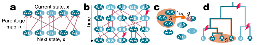
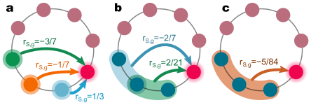
Figure 1: Modeling framework. a We consider a population of alleles at a specific locus, which can be of type $A$ or $a$. Each allele resides in a particular genetic site, within an individual. Each time-step, some alleles are replaced by copies of others, as a result of interaction, reproduction, mating, and/or death. This is recorded in a parentage map $\alpha$, indicating the parent allele of each site in the new state. b The process of selection is represented as a Markov chain. State transitions are determined by sampling a parentage map $\alpha$ from a probability distribution, which depends on the current state and captures all effects of social interaction, spatial structure, mating pattern, and so on. With mutation, there is a unique stationary distribution over states. c Multilateral genetic assortment is quantified by collective relatedness $r_{S,g}$, which characterizes the likelihood that site $g$ contains allele $A$ when all sites in set $S$ do. d Under neutral drift, collective relatedness can be computed via Eq. (3), using the expected branch lengths, $\ell_{S}$, of the tree representing $S$’s ancestry. The smaller the coalescence length $\ell_{S}$, the more likely that sites in $S$ contain the same allele.

We build upon a general mathematical framework for natural selection [34], which allows for arbitrary spatial and/or family structure, mating patterns, and fitness-affecting interactions (Appendix A; Fig. 1). There are two competing alleles, $A$ and $a$, at a single genetic locus. Taking a gene’s-eye view, we imagine a set $G$ of genetic sites, each housing one allele (Fig. 1a). Haploid individuals contain one site each, diploids two, and so on. The set of sites—and hence the population size—is fixed over time. The allele occupying each site $g\in G$ is indicated by a binary variable $x_{g}$, with value 1 if $g$ contains allele $A$ and 0 if $g$ contains $a$. The variables $x_{g}$ are collected into a binary vector $\mathbf{x}$ representing the population state.

Selection proceeds as a Markov chain. In each state $\mathbf{x}$, individuals may interact, migrate, mate, reproduce, and/or die. On the gene level, some alleles are replaced by copies of others, resulting in a new state, $\mathbf{x}^{\prime}$. The new allele in each site $g$ is either survived or copied from the allele previously occupying some other site, which we denote by $\alpha(g)$. Here, $\alpha$ is a parentage map [34]: a set mapping from $G$ to itself, indicating the site from which each allele is inherited (Fig. 1a). In each state $\mathbf{x}$, a probability distribution, over all possible parentage maps, captures the effects of all interactions—as well as all consequences of spatial structure, mating pattern, and inheritance (Mendelian or otherwise)—on the transmission of alleles to the next state.

Two parameters, $u$ and $\delta$, quantify the rate of mutation and the strength of selection, respectively. For nonzero mutation ($u>0$), the process converges to a stationary probability distribution over states $\mathbf{x}$. We say that selection favors allele $A$ if, in the low-mutation limit, $A$ has greater stationary frequency than $a$.

Collective relatedness

Selection for collective action depends on multilateral patterns of genetic assortment [24, 28]. To quantify these patterns, we introduce a measure of the collective relatedness of a set $S$ of sites to a single site $g$:

$$r_{S,g}=\lim_{u\to 0}\frac{\operatorname{\mathbb{E}}\left[\underline{x}_{S}\left(x_{g}-\bar{x}\right)\right]}{\operatorname{\mathbb{E}}\left[\bar{x}(1-\bar{x})\right]}.$$ (1)

Above, $\underline{x}_{S}=\prod_{h\in S}x_{h}$ has value 1 if all sites in $S$ contain allele $A$ and 0 otherwise, $\bar{x}=\frac{1}{n}\sum_{h\in G}x_{h}$ is the frequency of $A$, and $\operatorname{\mathbb{E}}$ denotes expectation over the stationary distribution. The numerator in Eq. (1) quantifies whether $g$ is more or less likely than an average site to contain allele $A$, when all of $S$ does. The denominator is the expected allelic variance in the population. As we show in Appendix D, Eq. (1) generalizes standard pairwise relatedness measures—based on covariance [23], identity-by-descent [25], and geometry [35]—and builds upon previous efforts to extend relatedness beyond pairs [21, 36].

Collective relatedness is difficult to evaluate for arbitrary selection strength, but can be systematically computed for neutral drift ($\delta=0$) using coalescent theory [37, 38]. The key quantity is the expected total branch length, $\ell_{S}$, of a tree representing the ancestry of a given set $S$ (Fig. 1d). These coalescence lengths, $\ell_{S}$, can be computed by solving the system of linear equations

$$\ell_{S}=\begin{cases}|S|+\sum_{\alpha}p(\alpha)\,\ell_{\alpha(S)}&|S|\geq 2\\ 0&|S|=1.\end{cases}$$ (2)

Above, $p(\alpha)$ is the probability that parentage map $\alpha$ occurs; under neutral drift, this probability not depend on the state $\mathbf{x}$. Collective relatedness under neutral drift is then given by

$$r_{S,g}=\frac{\bar{\ell}_{S}-\ell_{S\cup\{g\}}}{\bar{\ell}}.$$ (3)

Above, $\bar{\ell}_{S}$ is the average of $\ell_{S\cup\{h\}}$ as $h$ runs over all sites in $G$, and $\bar{\ell}$ is the average of $\ell_{\{h,k\}}$ over all pairs $h,k\in G$.

Condition for collective action

We represent collective action using collective fitness effects, $c_{S,g}$, that quantify how each set of sites $S$ affects the fitness of each site $g$. Specifically, if all sites in $S$ contain allele $A$, the fitness of each site $g$ (inside or outside of $S$) is altered by $c_{S,g}$, relative to the all-$a$ population state. Aggregating over all sets $S$, the net effect on $g$’s fitness in state $\mathbf{x}$ is $w_{g}(\mathbf{x})=\sum_{S\subseteq G}c_{S,g}\underline{x}_{S}$.

We prove in Appendix E that selection favors allele $A$ over $a$ if and only if

$$\sum_{g\in G}\sum_{S\subseteq G}c_{S,g}r_{S,g}>0.$$ (4)

This condition has two complementary interpretations. First, for a given site $g$, the sum $\sum_{S\subseteq G}c_{S,g}r_{S,g}$ characterizes the expected fitness effect of all social interactions experienced by an $A$ allele in site $g$. $A$ is favored if the total fitness effect on $A$ alleles, over all sites $g$, is positive. Second, for a particular set $S$ of sites, the sum $\sum_{g\in G}c_{S,g}r_{S,g}$ has the form of an inclusive fitness effect [11], in that $S$’s contribution, $c_{S,g}$, to the fitness of each site $g$, is weighted by collective relatedness, $r_{S,g}$. However, in contrast to standard inclusive fitness theory, the actor, $S$, is not an individual but a collective—a set of genetic sites whose joint actions affect their own fitness and that of others.

Condition (4) applies not only to collective action per se, but to any fitness-affecting interaction. The net effect of all interactions in state $\mathbf{x}$ on the fitness of each site $g$ can be written uniquely in the form [12] $w_{g}(\mathbf{x})=\sum_{S\subseteq G}c_{S,g}\underline{x}_{S}$, whereupon Condition (4) again determines which allele is favored.

Condition (4) is valid for any strength of selection $\delta>0$. For weak selection ($\delta\ll 1$), the collective relatedness coefficients $r_{S,g}$ can be evaluated using Eq. (3). This provides a method to evaluate weak selection on any nonlinear fitness-affecting behavior, with arbitrary spatial, network, group, and/or mating structure. If the collective fitness effects $c_{S,g}$ vanish for sets $S$ above a fixed size, this computation takes polynomial time.

Collective action among diploid relatives

JBS Haldane famously quipped that he would jump into a river to save two brothers, or eight cousins. Haldane’s insight is formalized in Hamilton’s rule [11, 13]: A behavior providing benefit $b$ to a relative, at cost $c$ to oneself, is favored if $br>c$, where $r$ quantifies relatedness between actor and recipient.

What about other interactions between relatives [21, 24]? Consider an arbitrary two-player game with two phenotypic strategies, Cooperate (C) and Defect (D). $AA$ individuals have phenotype C, $aa$’s have phenoptype D, and $Aa$ heterozygotes have phenotype C or D with probabilities $h$ and $1-h$, respectively, where $0\leq h\leq 1$ quantifies genetic dominance. The payoff to phenotype $X$ interacting with phenotype $Y$ is denoted $\pi_{XY}$, where $X$ and $Y$ can be either C or D. This game is played by two relatives in a large randomly-mating population. Their relationship is characterized by the probabilities, $p$ and $q$, that their maternally- and paternally-inherited alleles, respectively, descend from a recent common ancestor. For example, maternal half-siblings have $p=1/2$ and $q=0$. The average $r=(p+q)/2$ is Wright’s coefficient of relationship [39] (one-half for full siblings, one-eighth for cousins, etc.). Combining Eq. (3) and Condition (4) with standard results in coalescent theory [37, 38], we find (Appendix G) that weak selection favors allele $A$ (and hence cooperation) if

$$-c+br+\frac{2d(h-\tfrac{1}{2})(r-pq)}{3}>0.$$ (5)

Above $c=\frac{1}{2}(\pi_{\mathrm{DC}}+\pi_{\mathrm{DD}})-\frac{1}{2}(\pi_{\mathrm{CC}}+\pi_{\mathrm{CD}})$ is the cost of cooperation (averaged over the two phenotypes of interaction partners), $b=\frac{1}{2}(\pi_{\mathrm{CC}}+\pi_{\mathrm{DC}})-\frac{1}{2}(\pi_{\mathrm{CD}}+\pi_{\mathrm{DD}})$ is the benefit to the other, $d=\frac{1}{2}(\pi_{\mathrm{CC}}+\pi_{\mathrm{DD}})-\frac{1}{2}(\pi_{\mathrm{CD}}+\pi_{\mathrm{DC}})$ is the synergistic effect of both employing the same strategy. The first two terms recapitulate Hamilton’s rule, while the third captures the joint effects of synergy, $d$, and genetic dominance, $h$. The factor $r-pq$ is positive, unless the individuals are clonal ($p=q=1$) or unrelated ($p=q=0$), in which case it vanishes. Cooperation is therefore promoted if it is synergistic ($d>0$) and mostly dominant ($h>1/2$), or anti-synergistic ($d<0$) and mostly recessive ($h<1/2$). Although we describe this scenario in terms of cooperation, Condition (5) is valid for any two-player, two-strategy game.

What if Haldane must collaborate with one or more siblings to save another [33, 19]? Consider a collective of $m\geq 2$ full siblings. Each Cooperator in this collective pays cost $c/m$. Another sibling receives a benefit, $b_{k}$, depending on the number $k\leq m$ of Cooperators in the collective. Evaluating Condition (4), we find that weak selection favors cooperation if the benefit from all siblings helping exceeds twice the total cost: $b_{m}>2c$. Remarkably, this condition does not depend on the intermediate benefits, $b_{k}$ for $1\leq k\leq m-1$, nor on the degree of genetic dominance, $h$.

Finally, will siblings work together for a common benefit? Consider a threshold public goods game [2] played by $m$ siblings. Each Cooperator pays cost $c$. If all players cooperate, then each receives benefit $b$; otherwise, no benefits are received. We find that cooperation is favored if $2br_{m}>c$, where $r_{m}$ is the intra-relatedness of a collective of $m$ siblings (Table 1). For large $m$, this condition reduces to $b>2c$.

Table 1: Collective intra-relatedness, $r_{m}$, of $m$ full siblings in a diploid population

# of siblings, $m$	1	2	3	4	5
Arbitrary dominance, $h$	$\frac{1}{2}$	$\frac{17+2h}{48}$	$\frac{57+12h-4h^{2}}{192}$	$\frac{209+38h+12h^{2}-24h^{3}}{768}$	$\frac{801+104h+88h^{2}-32h^{3}-80h^{4}}{3072}$
Recessive ($h=0$)	$\frac{1}{2}$	$\frac{17}{48}$	$\frac{19}{64}$	$\frac{209}{768}$	$\frac{267}{1024}$
No dominance ($h=\tfrac{1}{2}$)	$\frac{1}{2}$	$\frac{3}{8}$	$\frac{31}{96}$	$\frac{19}{64}$	$\frac{433}{1536}$
Dominant ($h=1$)	$\frac{1}{2}$	$\frac{19}{48}$	$\frac{65}{192}$	$\frac{235}{768}$	$\frac{881}{3072}$

Collective action on networks and hypergraphs

Network structure—representing spatial or social relationships—has a profound effect on the evolution of social behavior [26, 27, 29]. Exact mathematical results have been derived for pairwise interactions [27, 29], but are difficult to obtain for interactions beyond pairs [30, 28, 32].

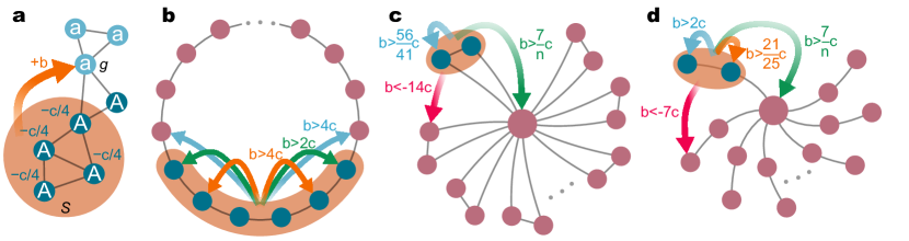
To apply our framework, we let $G$ be the set of nodes in a network. Each node represents an individual, with a single heritable type. As a simple model of collective action, suppose that a particular collective $S$, of size $m$, may help or harm a particular node $g$—inside or outside $S$—at some cost to $S$’s members (Fig. 2a). Individuals in $S$ may pay $c/m$ each to contribute to the action, where $c>0$ represents the action’s total cost. If all individuals in $S$ contribute, the payoff of target node $g$ is altered by an amount $b$; otherwise, there is no effect. Collective help is the case $b>0$, while $b<0$ indicates collective harm. Reproduction occurs via death-Birth updating [26, 27, 29]: First, a site is chosen uniformly from the population to be replaced; then, a neighbor is chosen with probability proportional to $\left(\text{payoff}\right)\times\left(\text{edge weight}\right)$ to reproduce into the vacancy.

Applying Condition (4) (see Appendix H), weak selection favors this collective help or harm if

$$bd_{g}\left(r_{S,g}-r_{S,g}^{(2)}\right)>\frac{c}{m}\sum_{h\in S}d_{h}\left(r_{h}-r_{h}^{(2)}\right).$$ (6)

Above, $d_{g}$ is the degree of node $g$, $r_{S,g}^{(2)}$ is the expected collective relatedness of $S$ to two-step random walk neighbors of $g$, $r_{h}=r_{\{h\},h}$ is the self-relatedness of site $h$, and $r_{h}^{(2)}=r^{(2)}_{\{h\},h}$ is the expected relatedness of $h$ to its own two-step random walk neighbors. The left-hand side of Condition (6) compares the effect of collective action on the target $g$ (weighted by collective relatedness from $S$) to that on $g$’s two-step neighbors, who compete with $g$ for opportunities to reproduce. The right-hand side quantifies the effects of costs paid, and is never negative.

Collective $S$ can be favored to help node $g$ if $r_{S,g}>r_{S,g}^{(2)}$; that is, if $S$ is more related to $g$ than to $g$’s two-step neighbors. In this case, help is favored if the benefit-cost ratio $b/c$ exceeds the threshold

$$(b/c)_{S,g}^{*}=\frac{\sum_{h\in S}d_{h}\left(r_{h}-r_{h}^{(2)}\right)}{md_{g}\left(r_{S,g}-r_{S,g}^{(2)}\right)}.$$ (7)

In contrast, if $r_{S,g}<r_{S,g}^{(2)}$, then collective help is never favored, and collective harm ($b<0$) is favored if $b/c<(b/c)_{S,g}^{*}$. If $r_{S,g}=r_{S,g}^{(2)}$ (in particular, if $g$ and all of its two-step neighbors are within $S$) then $S$ cannot be favored to help or harm $g$.

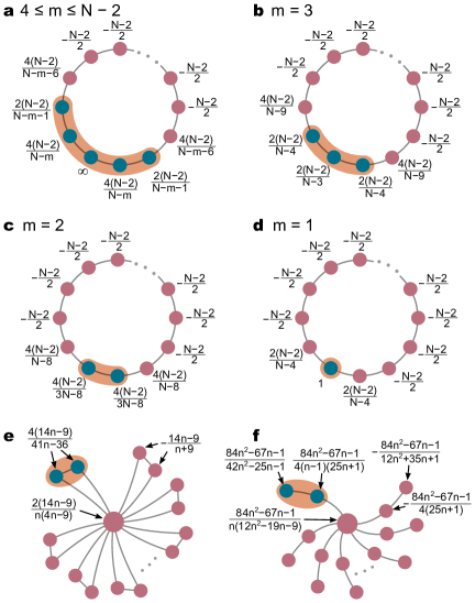
Figure 2: Collective action on simple networks. a We consider a scenario in which a collective $S$ of $m$ network nodes may help a particular node $g$. $A$ individuals within $S$ pay cost $c/m$ each; if all pay, then $g$ receives benefit $b$. b For a large cycle network, a connected collective of size at least four is favored to help its own boundary nodes if $b>2c$, and the neighbors of these boundary nodes if $b>4c$. c On a windmill network with $n\gg 1$ blades, a blade is favored to help the hub if $nb>7c$, which can be satisfied even if the benefit is negligible compared to the cost. In contrast, help to a node within the blade is only favored if $b>\frac{56}{41}c$. Harmful behavior can be favored toward nodes in other blades, if $b<-14c$. d The “spider” network displays similar behavior to the windmill, but help is more readily favored to the inner node of a leg ($b>\frac{21}{25}c$) than to the outer leg ($b>2c$). Results shown here are for large networks; finite-size results are given in Extended Data Figure 6.

Using Condition (6), we can determine whether any set of nodes on a given network is favored to help or harm any target. On a large cycle (Fig. 2b, Extended Data Figure 6a–d), a collective of four or more connected nodes is favored to help its own boundary node if $b>2c$, or the two neighbors of a boundary node if $b>4c$. Neither help nor harm can be favored to any other node.

On heterogeneous networks (Figs. 2cd, Extended Data Figure 6ef), selection can favor extreme collective altruism, in which the benefit is negligible compared to the cost. This occurs when the target is a highly-connected neighbor; such “hubs” are critical for the spread of alleles. Toward other targets, collective harm can be favored. A windmill blade (Fig. 2c) is favored to harm a node in another blade if $b<-14c$, and a spider leg (Fig. 2d) is favored to harm the outer node of another leg if $b<-7c$.

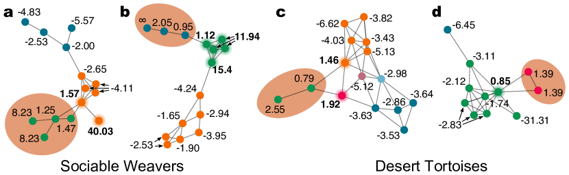
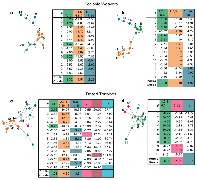
For real-world networks of sociable weavers [40] (Philetairus socius) and desert tortoises [41] (Gopherus agassizii), small, isolated subcommunities are often favored to help their neighbors, and occasionally their neighbors-of-neighbors (Fig. 3 and Extended Data Figure 7). In some cases, help can be favored even if the benefit is less than the cost. Larger and more centralized subcommunities, in contrast, show only potential for collective harm.

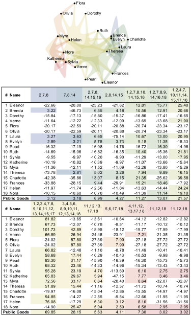
Figure 3: Collective action on animal networks. We partitioned networks into subcommunities using the Girvan-Newman algorithm [42]. Critical benefit-cost thresholds $(b/c)_{S,g}^{*}$, from each subcommunity to each target, were computed according to Eq. (7). Positive (resp., negative) values indicate potential for collective help (resp., harm); this help or harm is selected if the benefit-cost ratio exceeds $(b/c)_{S,g}^{*}$ in absolute value. Results are shown here for particular subcommunities (indicated by ovals); results for all subcommunities are shown in Extended Data Figure 7. a,b Two co-nesting networks of Philetairus socius [40]. In a, the collective is favored to help its neighbor whenever $b/c>1.57$, a lower threshold than for two of its own members. The collective in b can be favored to help all of its neighbors up to distance 2, but not one of its own members (because this member is irrelevant of the spread of the collective’s alleles). c,d Co-burrowing networks of Gopherus agassizii [41]. In c, help to one of the collective members is favored if $b/c>0.79$, meaning the benefit may be less than the cost. In d, such net-negative help can be favored to a neighbor of the collective.

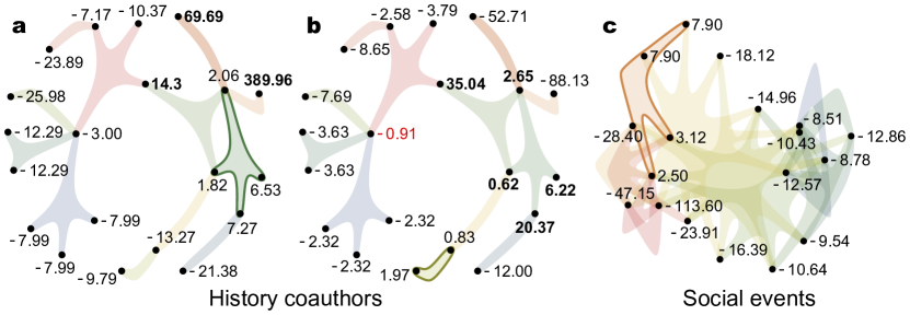
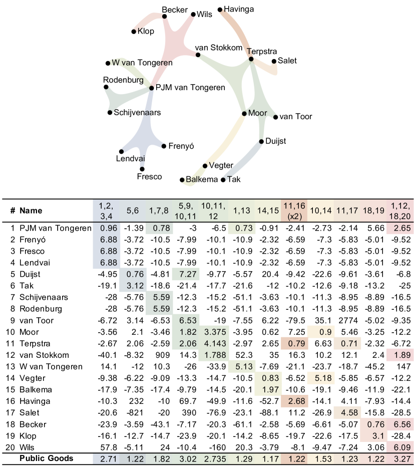
We also analyze collective action by hyperedges—representing multilateral human relationships—on real-world hypergraphs [43, 32] (Fig. 4). In this context, behaviors spread to neighbors via imitation, rather than genetic transmission. For an academic coauthorship hypergraph [43] (Fig. 4ab, Extended Data Figure 8), we again find that the propensity to help neighbors—and neighbors-of-neighbors—decreases with collective size. Collective harm can be favored to more distant individuals, even (in one case) when the damage inflicted is less than the cost. For a hypergraph representing attendance at social events [44] (Fig. 4c, Extended Data Figure 9), which is more densely interconnected, no hyperedge is favored to help any individual outside the hyperedge.

Figure 4: Collective action on hypergraphs We computed critical benefit-cost thresholds for collective action, $(b/c)^{*}_{S,g}$, for hypergraphs representing coauthorship of history research articles [43], and co-attendance at social events [44]. Results for particular hyperedges are shown here; see Extended Data Figures 8 and 9 for all hyperedges and targets. a For the coauthorship hypergraph, a four-node hyperedge can be selected to help neighbors, but only for benefit/cost ratios of at least 14.3. b A two-node hyperedge is favored to help its neighbor if $b>0.62c$, and help to neighbors-of-neighbors can be favored as well. Toward other nodes, selection can favor collective harm—in one case this requires only $b<-0.91c$. c For the social event hypergraph, which is more densely interconnected, no hyperedge is favored to help others.

Synergy and collective actors

The evolution of social behavior is typically studied at the level of individual actors. Natural selection is believed to lead individuals to act as if trying to maximize their inclusive fitness [11, 20]—a sum of fitness effects weighted by relatedness to each recipient. However, multilateral, synergistic interactions make it difficult to identify the inclusive fitness of any given individual [13, 20].

Condition (4) resolves this difficulty by expanding the notion of “actor” to include collectives. Each synergistic effect is ascribed to a collective actor $S$, comprising all sites involved in the synergy. The resulting consequences for selection are captured by $S$’s “collective inclusive fitness effect”, $w_{S}^{\mathrm{IF}}=\sum_{g\in G}c_{S,g}r_{S,g}$. Here, $r_{S,g}$ quantifies $S$’s shared genetic interest (positive or negative) in site $g$’s fitness. To separate $S$’s effects on its own members versus outsiders, $w_{S}^{\mathrm{IF}}$ can be decomposed as $r_{S}\sum_{g\in S}c_{S,g}+\sum_{g\notin S}c_{S,g}r_{S,g}$, where $r_{S}=\lim_{u\to 0}\left(\operatorname{\mathbb{E}}\left[\underline{x}_{S}-\underline{x}_{S}\bar{x}\right]/\operatorname{\mathbb{E}}\left[\bar{x}(1-\bar{x})\right]\right)$ is the common value of $r_{S,g}$ for all members $g$ of $S$. This “intra-relatedness”, $r_{S}$, is always positive, and exceeds $r_{S,g}$ for any $g$ outside of $S$.

Selection favors an allele if the total inclusive fitness effect of all collectives is positive, $\sum_{S\subseteq G}w^{\mathrm{IF}}_{S}>0$. Although every subset of sites $S$ is included in this total, only those with non-negligible intra-relatedness, $r_{S}$, and synergistic effects, $c_{S,g}$, contribute appreciably to selection.

Figure 5: Conflicting inclusive fitness interests within a collective a On a cycle of size 8, three consecutive sites have conflicting relatedness values to a neighboring target site (indicated in red). The closest site has positive relatedness to the target, indicating potential for helpful behavior, while the other two have negative relatedness, indicating potential for harm. b For neighboring pairs of sites, collective relatedness to the target is positive for the nearer pair but negative for the further pair. c Taken together, the three sites have negative collective relatedness to the target. The outcome of selection reflects an aggregation over these differing individual and collective interests, as quantified by Condition (4).

Does selection lead collectives to act as if trying to maximize inclusive fitness? In one highly idealized case, yes. Suppose that a mutant allele affects the actions of only a single collective $S$. We prove that weak selection favors this mutant allele if and only if it increases the quantity $\sum_{g\in G}w_{g}(\mathbf{x})\,r_{S,g}$, which can be interpreted as $S$’s inclusive fitness. In this way, selection would lead $S$ to act as if maximizing inclusive fitness, if the actions of all other collectives (including those contained in or overlapping with $S$) were held fixed. Although conceptually appealing, this result has limited applicability. It is unclear how an allele could affect the actions of only a single collective, and not that of its members or overlapping sets. Moreover, the inclusive fitness interests of a collective can differ from those of its members or subsets (Fig. 5), making simultaneous maximizing behavior impossible. Instead, divergent interests create the potential for evolutionary conflict, such as over worker reproduction in ant colonies [45]. Selection, according to Condition (4), leads not to maximizing behavior, but to conflict and compromise over competing individual and collective prerogatives.

Outlook

Our work provides a mathematical theory for how the actions of collectives, toward their own members and/or others, are shaped by natural selection. Our main result, Condition (4), shows how selection for collective action—or any other social behavior—depends on genetic assortment (quantified by $r_{S,g}$) and synergy (quantified by $c_{S,g}$). This genetic assortment can arise from interactions within families or groups, or from spatial clustering on networks and hypergraphs. Small, isolated communities show the greatest propensity to evolve collective help toward neighbors.

A robust field of research [46, 47] has demonstrated how collective action is achieved via interactions among individuals. Our results complement this research by illuminating why, and when, such collective action evolves.

The notion of collective actors introduced here provides new evolutionary grounding for the idea of shared agency [48]. Moreover, since every multicellular organism is a collection of cells, and every genome a collection of genes, the origin of multicellularity [49] and other transitions in individuality [50] can be understood as the emergence of radical new forms of collective action. In this sense, all action is collective action.

Data availability

No datasets were generated in this work. We made use of publicly available datasets from the Network Data Reposity [51] (http://networkrepository.com/), UCINet [52] (https://sites.google.com/site/ucinetsoftware/datasets), and Austin R. Benson [43] (https://www.cs.cornell.edu/~arb/data/).

Code availability

Coalescence lengths and benefit-cost thresholds on networks and hypergraphs were computed using MATLAB (version R2022a). Code is available at https://github.com/Emmanuel-Math-Bio-Research-Group/Collective-Action. To implement the Girvan-Newman algorithm we used the UCINet [52] software package (v6.753), available at https://sites.google.com/site/ucinetsoftware/.

Author Contributions

BA conceived the project. BA, AK, JD, YAD, and CS analyzed the model. BA and CL designed the figures. BA, YAD, and CS supervised student researchers. BA wrote the manuscript.

Extended Data Figure 6: Benefit-cost thresholds for collective action on finite cycles, windmills, and spiders. a-d For a cycle of size $N$, critical benefit-cost thresholds $(b/c)^{*}_{S,g}$ are shown for all possible collectives of size $1\leq m\leq N-2$ and all possible targets. Separate cases are needed for collectives of size less than four. e For a Windmill graph with $n$ “blades”, critical benefit-cost thresholds $(b/c)^{*}_{S,g}$ are shown a collective $S$ consisting of the two vertices on a single blade, and all possible targets. e For a Spider graph with $n$ “legs”, critical benefit-cost thresholds $(b/c)^{*}_{S,g}$ are shown for a collective $S$ consisting of the two vertices on a single leg, and all possible targets. Note that, for both the Windmill and Spider graphs, the benefit-cost threshold to the hub is asymptotically $7/n$, and in particular approaches zero for large $n$. All calculations are provided in the Supplementary Information.

Extended Data Figure 7: Collective action on animal networks Networks were obtained from the Network Data Repository [51] and partitioned into subcommunities using the Girvan-Newman algorithm [42]. Benefit-cost thresholds $(b/c)^{*}_{S,g}$ are shown for each subcommunity $S$ and node $g$. “Public goods” refers to a scenario in which each member of $S$ may choose to pay cost $c$; if all do, then each receives benefit $b$, otherwise no benefits are received. Cooperation (i.e. paying the cost) is favored if $b/c$ exceeds the threshold of $(b/c)_{S}^{*}=\left(\sum_{g\in S}d_{g}\left(r_{g}-r_{g}^{(2)}\right)\right)/\left(\sum_{g\in S}d_{g}\left(r_{S,g}-r_{S,g}^{(2)}\right)\right)$. a, b Co-nesting networks of sociable weavers (Philetairus socius) obtained by van Dijk et al. [40]. c, d Co-burrowing networks of desert tortoises (Gopherus agassizii) obtained by Sah et al. [41].

Extended Data Figure 8: Collective action on a history co-authorship hypergraph A connected component of a hypergraph representing co-authorship of academic history articles, obtained by Benson et al. [43] from the Microsoft Academic Graph [53]. The hyperedge $\{\text{Terpstra, Balkema}\}$ is doubly weighted because there are two papers with these coauthors. Benefit-cost thresholds $(b/c)^{*}_{S,g}$ are shown for each hyperedge $S$ and node $g$, and also for the public goods scenario described in the caption of Extended Data Figure 7.

Extended Data Figure 9: Collection action on the Southern Women hypergraph A record of attendance at social gatherings by women in Natchez, Mississippi, USA in the 1930’s [44] is represented as a hypergraph, with each hyperedge corresponding to one social event. The hyperedge $\{\text{Sylvia, Katherine, Nora}\}$ is repeated because there were two events with these attendees. Benefit-cost thresholds $(b/c)^{*}_{S,g}$ are shown for each hyperedge $S$ and node $g$, and also for the public goods scenario described in the caption of Extended Data Figure 7.

Appendix

This appendix contains a full mathematical description of our modeling framework, proofs of our main results, computation of examples, and comparisons to previous work. The derivations are mostly self-contained, with only a few reliances on results proven in previous works [54, 55, 34, 56, 57]. We assume familiarity with discrete mathematics (sets, relations, functions, etc.) [58] and probability, especially finite Markov chains [59]. Readers may also refer to Refs. [55, 34] for a more pedagogical exposition of the kind of mathematical framework used here.

Section A presents our mathematical modeling framework. Sections B and C prove key mathematical results, culminating in a proof of equivalence between various criteria for selection (Theorems C.2 and C.3). Section D presents our definition of collective relatedness, and its relationship to other assortment measures such as coalescence length and identity-by-descent. Our main result regarding collective action is proven in Section E, Theorems E.1 and E.2. Our result on maximization of collective inclusive fitness (in a highly idealized case) is proven in Section F. Finally, we develop the application of our main results to collective action among diploid relatives (Section G) and on networks and hypergraphs (Section H).

Appendix A Modeling framework

We start by introducing the modeling framework from which our results are derived. The framework presented here is a variant on one developed in earlier works [55, 34, 56, 57]. It describes a population of fixed size and spatial structure, which may be haploid, diploid, or otherwise. The relationship to previous formulations of this framework is discussed in Section A.9.

A.1 Set-theoretic notation

We will use standard set-theoretic notation throughout: $\in$ for element, $\subseteq$ for subset, and $\varnothing$ for empty set. The cardinality (size) of a finite set $S$ is denoted $|S|$. For two sets $S$ and $T$, we let $S^{T}$ denote the set of all $T$-indexed tuples of the form $(s_{t})_{t\in T}$, with each $s_{t}\in S$.

For a set mapping $f:S\to T$, we denote the image of a subset $S^{\prime}\subseteq S$ by $f(S^{\prime})\subseteq T$, and the preimage of a subset $T^{\prime}\subseteq T$ by $f^{-1}(T^{\prime})\subseteq S$. We also use the shorthand $f^{-1}(t)=f^{-1}(\{t\})$ for the preimage of a singleton subset $\{t\}\subseteq T$.

A.2 Genetic sites and individuals

Adopting a gene’s-eye view, we consider a population of alleles at a particular genetic locus. There is a set $G$ of genetic sites at which alleles can reside; each site houses a single allele. The total number of sites is denoted $n=|G|$.

The individuals in the population are represented by a fixed set $I$. The set $G$ of genetic sites is partitioned into subsets $G_{i}$, for each $i\in I$, representing the sites contained in individual $i$. The number of sites in individual $i$, denoted $n_{i}=|G_{i}|$, corresponds to $i$’s ploidy ($n_{i}=1$ if $i$ is haploid, $n_{i}=2$ if diploid, and so on).

A.3 Alleles and states

There are two competing allele types, $A$ and $a$, which are assigned numerical values 1 and 0, respectively. The allele type occupying each site $g\in G$ is indicated by a binary variable $x_{g}\in\{0,1\}$. The overall population state is the binary vector $\mathbf{x}=(x_{g})_{g\in G}$. The set of all possible states is $\{0,1\}^{G}$.

A.4 Transitions

A transition from one state to another involves two components. The first is a set mapping $\alpha:G\to G$, indicating the site from which each allele in the new state is inherited (in the case of new offspring) or retained (if the allele survives). Thus $\alpha(g)=h$, for $g,h\in G$, indicates that the new occupant of site $g$ is the same as, or a copy of, the allele that occupied site $h$ in the previous time-step. Our framework does not formally distinguish between these two possibilities, as they both result in transmission an allele from $g$ to $h$. We call $\alpha$ the parentage map, understanding a surviving allele to be its own “parent”.

The second component is the subset $U\subseteq G$ of sites that undergo mutation during the transition. In general, $U$ can be any subset of $G$, including the empty set $\varnothing$ (indicating that no mutations occur).

The probability that parentage map $\alpha$ and mutation set $U$ occur in state $\mathbf{x}$ is denoted $p_{\mathbf{x}}(\alpha,U)$. For each state $\mathbf{x}$, $\{p_{\mathbf{x}}(\alpha,U)\}_{(\alpha,U)}$ comprises a joint probability distribution on the set of possible combinations of $\alpha$ and $U$.

We allow the probabilities $p_{\mathbf{x}}(\alpha,U)$ to depend on the state $\mathbf{x}$ in an arbitrary way, subject only to a Fixation Axiom introduced in the next subsection. In this way, our framework encompasses a wide variety of models of selection. Spatial, network, or group structure, behavioral interactions, migration, mate choice, and allele transmission (Mendelian or not) are all represented implicitly in the probability distributions $p_{\mathbf{x}}$.

We denote the marginal probabilities of a parentage map $\alpha$ and a mutation set $U$, respectively, by

$$p_{\mathbf{x}}(\alpha)=\sum_{U\subseteq G}p_{\mathbf{x}}(\alpha,U)\qquad\text{and}\qquad p_{\mathbf{x}}(U)=\sum_{\alpha:G\to G}p_{\mathbf{x}}(\alpha,U).$$ (A.1)

We also use the notation $\operatorname{\mathbb{P}}_{\mathbf{x}}$ and $\operatorname{\mathbb{E}}_{\mathbf{x}}$ for probabilities and expectations, respectively, under the distribution $\{p_{\mathbf{x}}(\alpha,U)\}_{(\alpha,U)}$ for a given state $\mathbf{x}$. For example, the expected number of (self + offspring) of site $g\in G$, in a single transition from state $\mathbf{x}$, can be written as $\operatorname{\mathbb{E}}_{\mathbf{x}}[|\alpha^{-1}(g)|]$.

A.5 Fixation Axiom

For the population to evolve as a unit, it should be possible for at least one genetic site to spread its progeny throughout the population. We formalize this with the following axiom:

Fixation Axiom.

There exists a site $g\in G$ such that, for each $h\in G$, there is a finite sequence of parentage maps $\alpha_{1},\ldots,\alpha_{m}$ with $p_{\mathbf{x}}(\alpha_{k})>0$ for each $k=1,\ldots,m$ and $\mathbf{x}\in\{0,1\}^{G}$, and $\alpha_{1}\circ\cdots\circ\alpha_{m}(h)=g$.

A.6 Selection Markov chain

A particular model within our framework is defined by a set $G$ and a collection of probability distributions $p_{\mathbf{x}}$ for each state $\mathbf{x}\in\{0,1\}^{G}$, satisfying the Fixation Axiom. Given these ingredients, the process of selection is represented as a Markov chain on $\{0,1\}^{G}$. We call this the selection Markov chain, denoted $\mathcal{M}=(\mathbf{X}^{t})_{t=0}^{\infty}$. The initial state $\mathbf{X}^{0}$ may be chosen arbitrarily. For all subsequent times $t\geq 1$, state $\mathbf{X}^{t}$ is constructed from $\mathbf{X}^{t-1}$ by first sampling a parentage map $\alpha^{t}$ and mutation set $U^{t}$ from $p_{\mathbf{X}^{t}}$, and then, for each $g\in G$, setting

$$X^{t}_{g}=\begin{cases}X^{t-1}_{\alpha^{t}(g)}&g\notin U^{t}\\ 1-X^{t-1}_{\alpha^{t}(g)}&g\in U^{t}.\end{cases}$$ (A.2)

In particular, if there is no mutation (that is, if $p_{\mathbf{x}}(\varnothing)=1$ for all $\mathbf{x}\in\{0,1\}^{G}$) then $X^{t}_{g}=X^{t-1}_{\alpha^{t}(g)}$ for all $g\in G$. We can write this compactly as

$$\mathbf{X}^{t}=\mathbf{X}^{t-1}_{\alpha^{t}},$$ (A.3)

where, for any state $\mathbf{x}\in\{0,1\}^{G}$ and set mapping $\sigma:G\to G$, $\mathbf{x}_{\sigma}$ denotes the state with allele $x_{\sigma(g)}$ in each site $g\in G$.

For some purposes, it will be useful to include the parentage mapping $\alpha^{t}$ and mutation set $U^{t}$ as part of the Markov chain state. For this, we define the augmented Markov chain $\tilde{\mathcal{M}}$ with states $(\mathbf{X}^{t},\alpha^{t},U^{t})$, with $\mathbf{X}^{t}$, $\alpha^{t}$ and $U^{t}$ as defined above. The initial state $(\mathbf{X}^{0},\alpha^{0},U^{0})$ of $\tilde{\mathcal{M}}$ may be chosen arbitrarily.

A.7 Mutation and selection parameters

In order to vary the effects of mutation and selection, we allow the probabilities $p_{\mathbf{x}}(\alpha,U)$ to additionally depend on two parameters: a mutation parameter $u$ with $0\leq u\leq 1$, and a selection intensity parameter $\delta$ with $0\leq\delta\leq\epsilon$ for some $\epsilon>0$. In addition to requiring that the Fixation Axiom be satisfied for all combinantions of $u$ and $\delta$, we impose the following additional assumptions on the behavior of the probability distributions $p_{\mathbf{x}}$ with respect to these parameters.

The first is a differentiability requirement:

• Each probability $p_{\mathbf{x}}(\alpha,U)$ is jointly twice-differentiable, with continuous second partial derivatives, in both $u$ and $\delta$

Second $\delta=0$ should represent neutral drift. This means that alleles $A$ and $a$ should be interchangeable, and thus the probability distribution on $\alpha$ and $U$ should be independent of the state:

• For $\delta=0$, the probabilities $p_{\mathbf{x}}(\alpha,U)$ are independent of $\mathbf{x}$.

Third, no mutation should occur in the case $u=0$:

• For $u=0$, $p_{\mathbf{x}}(U)=0$ for all $U\neq\varnothing$.

Fourth, when $u>0$, it should be possible for new mutations to arise and sweep to fixation:

• For $u>0$, there exists some $g\in G$, satisfying the conditions of the Fixation axiom, such that $\operatorname{\mathbb{P}}_{\mathbf{x}}[g\in U]>0$.

Fifth, the probability of multiple mutations should be of order $u^{2}$ as $u\to 0$.

• For each $\mathbf{x}\in\{0,1\}^{G}$ and each fixed $\delta\geq 0$, $\lim_{u\to 0}\frac{\operatorname{\mathbb{P}}_{\mathbf{x}}[|U|\geq 2]}{u}=0$.

Sixth, since $u$ is intended to only parameterize mutation, the marginal probability of each parentage map in a given state should be independent of $u$:

• For each $\alpha:G\to G$ and each $\mathbf{x}\in\{0,1\}^{G}$, $p_{\mathbf{x}}(\alpha)$ is independent of $u$.

Seventh, for $u<1$, it should be possible for no mutation to occur:

• For $u<1$ and all $\mathbf{x}\in\{0,1\}$, $\operatorname{\mathbb{P}}_{\mathbf{x}}[U=\varnothing]>0$.

Finally, in order to isolate the effects of selection, we assume that probabilities of mutation are the same in the two monoallelic states:

• For each $U\subseteq G$ and $u\geq 0$, $p_{\mathbf{a}}(U)=p_{\mathbf{A}}(U)$.

Assumption (M6) removes the possibility that mutation can favor one trait over another; thus any differences in the frequency of $A$ versus $a$ must be due to selection alone. Without (M6), the effects of mutation and selection are difficult to disentangle [60].

A.8 Phenotypes

Although most of our analysis will be conducted on the gene level, it will in some cases be useful to employ a notion of individual phenotype. For this, we suppose there are two phenotypes, numbered 1 and 0. The phenotype $\Phi_{i}\in\{0,1\}$ of each individual $i\in I$ is determined stochastically based on the vector $\mathbf{x}_{|G_{i}}=(x_{g})_{g\in G_{i}}$ of alleles present in this individual. Specifically, each individual $i$ has phenotype 1 with some probability $\varphi_{i}(\mathbf{x}_{|G_{i}})$, and otherwise has phenotype 0. We require that individuals with only $A$ alleles always have phenotype 1, $\varphi_{i}(1,\ldots,1)=1$, and those with only $a$ alleles always have phenotype 0, $\varphi_{i}(0,\ldots,0)=0$. Each individual’s phenotype is determined independently of all others’.

For example, suppose $i$ is a diploid individual, with genetic sites $G_{i}=\{i_{1},i_{2}\}$. Let $0\leq h\leq 1$ represent the degree of genetic dominance, so that an $Aa$ heterozygote has phenotype 1 or 0 with probability $h$ or $1-h$, respectively. Then the probability $\varphi_{i}(\mathbf{x}_{|G_{i}})$ that $i$ has phenotype 1 can be expressed as:

$$\operatorname{\mathbb{P}}_{\mathbf{x}}[\Phi_{i}=1]=\varphi_{i}(x_{i_{1}},x_{i_{2}})=h\left(x_{i_{1}}+x_{i_{2}}\right)+(1-2h)x_{i_{1}}x_{i_{2}}.$$ (A.4)

We observe that $\varphi_{i}(1,1)=1$, $\varphi_{i}(0,0)=0$, and $\varphi_{i}(1,0)=\varphi_{i}(0,1)=h$, as required.

We collect the phenotypes of all individuals into a vector $\mathbf{\Phi}=(\Phi_{i})_{i\in I}$, representing the phenotypic state of the population. The phenotypic state $\mathbf{\Phi}$ depends stochastically on the genotypic state $\mathbf{x}$, according to the probabilities $\varphi_{i}(\mathbf{x}_{|G_{i}})$.

The probability that transition event $(\alpha,U)$ occurs in phenotypic state $\mathbf{\Phi}$ is denoted $\hat{p}_{\mathbf{\Phi}}(\alpha,U)$. Here and below, a hat is used to indicate quantities that depend on the phenotypic state $\Phi$ rather than the genotypic state $\mathbf{x}$.

The phenotype-level formalism discussed in this subsection is a special case of the gene-level framework introduced earlier. The gene-level framework can be recovered from the phenotypic one by setting $p_{\mathbf{x}}(\alpha,U)=\operatorname{\mathbb{E}}_{\mathbf{x}}\left[\hat{p}_{\mathbf{\Phi}}(\alpha,U)\right]$, with expectation taken over the probability distribution on $\mathbf{\Phi}$ in state $\mathbf{x}$.

A.9 Relationship to prior frameworks

The framework introduced here is closely related to those developed in previous works [55, 34, 56, 57], especially Ref. [34]. There are, however, two key differences to highlight.

First, we do not explicitly record births and deaths in the present framework. That is, we make no formal distinction between an allele surviving into the next generation versus being replaced by a copy of itself. This simplifies notation, and also allows for surviving alleles to move between sites (e.g. via migration of adult individuals), which was not allowed in previous formulations.

Second, we do not specify any particular relationship between reproduction and mutation. Previous formulations assumed that offspring alleles acquire mutations independently with some fixed probability. By instead allowing for an arbitrary joint probability distribution on the set $U$ of mutated sites and the parentage map $\alpha$, we allow for mutation of surviving alleles, mutation rates that vary across sites, and non-independence of mutation events in a particular state.

Despite these differences, some results proven in previous works [55, 34, 56, 57] carry over to the present framework with minimal modification, and will be invoked without proof.

Appendix B Stationarity and fixation

In this section we establish the long-term behavior of the selection Markov chain $\mathcal{M}$. The case of no mutation is particularly important; we therefore introduce the notation $\mathcal{M}_{0}$ for the $u=0$ case of $\mathcal{M}$.

B.1 Asymptotic behavior of the selection Markov chain

There are two cases for the asymptotic behavior of the selection Markov chain $\mathcal{M}$ depends on the mutation parameter $u$. For $u=0$, the population is eventually taken over by one of the two competing alleles, while for $u>0$, there is a unique stationary distribution, $\pi_{\mathcal{M}}$. We formalize these observations in the following theorem:

Theorem B.1.

$\mathcal{M}_{0}$ has absorbing states $\mathbf{a}$ and $\mathbf{A}$, and all other states are transient in $\mathcal{M}_{0}$. For $0<u<1$, $\mathcal{M}$ has a unique stationary distribution, $\pi_{\mathcal{M}}$, that satisfies

$$\lim_{t\to\infty}\operatorname{\mathbb{P}}[\mathbf{X}^{t}=\mathbf{x}|\mathbf{X}^{0}=\mathbf{y}]=\pi_{\mathcal{M}}(\mathbf{x}),$$ (B.1)

for any pair of states $\mathbf{x},\mathbf{y}\in\{0,1\}^{G}$.

Proof.

The claim regarding $\mathcal{M}_{0}$ is Theorem 1 of Allen and Tarnita [55]. For the $0<u<1$ case, it suffices to show that $\mathcal{M}$ has a unique closed communicating class, and is aperiodic on this class. Consider an arbitrary initial state $\mathbf{X}^{0}=\mathbf{y}$. We will show that states $\mathbf{A}$ and $\mathbf{a}$ are both accessible from $\mathbf{y}$, which will prove that $\mathcal{M}$ has a unique closed communicating class containing $\mathbf{A}$ and $\mathbf{a}$. Consider a site $g\in G$ and sequence $\alpha_{1},\ldots,\alpha_{k}$ satisfying the properties specified in the Fixation Axiom and Assumption (M2). Suppose the transition events $(\alpha_{1},\varnothing),\ldots,(\alpha_{k},\varnothing)$ all occur in sequence from initial state $\mathbf{y}$; this sequence has positive probability by (M5) and the assumed properties of $g$. The resulting state is $\mathbf{a}$ or $\mathbf{A}$, respectively, if $y_{g}=0$ or $y_{g}=1$. Now suppose the next transition event has $g\in U$ (this has positive probability by Assumption (M2)), and that the sequence $(\alpha_{1},\varnothing),\ldots,(\alpha_{k},\varnothing)$ again follows afterwards. The resulting state is now either $\mathbf{A}$ or $\mathbf{a}$, respectively, if $y_{g}=0$ or $y_{g}=1$. In either case, both $\mathbf{A}$ and $\mathbf{a}$ are accessible from $\mathbf{y}$, and therefore $\mathcal{M}$ has a unique closed communicating class.

Aperiodicity follows from the fact that $\operatorname{\mathbb{P}}_{\mathbf{A}}[U=\varnothing]$ and $\operatorname{\mathbb{P}}_{\mathbf{a}}[U=\varnothing]$ are both positive by Assumption (M5); any transition event with $U=\varnothing$ in state $\mathbf{a}$ or $\mathbf{A}$ leaves the state unchanged. ∎

B.2 Ancestral mapping

Here we introduce a family of stochastic mappings that record ancestral lineages in the selection Markov chain.

Definition.

In $\tilde{\mathcal{M}}$, for any pair of times $t_{0}$ and $t$ with $0\leq t_{0}<t$, we define the ancestral mapping $A_{t_{0}}^{t}:G\to G$ by

$$A_{t_{0}}^{t}=\alpha^{t_{0}+1}\circ\alpha^{t_{0}+2}\circ\cdots\circ\alpha^{t}.$$ (B.2)

For $t_{0}=t$ we define $A_{t}^{t_{0}}$ to be the identity mapping on $G$.

In words, site $A_{t_{0}}^{t}(g)\in G$ contains the ancestor, at time $t_{0}$, of the allele occupying site $g\in G$ at time $t$. Conversely, the preimage $(A_{t_{0}}^{t})^{-1}(g)\subseteq G$ identifies the locations of descendants, at time $t$, of the allele occupying site $g$ at time $t_{0}$. In the $t_{0}=t$ case, each allele’s “ancestor” is itself—that is, $A_{t}^{t}(g)=g$.

Absent mutation, each allele is a faithful copy of its ancestor. Accordingly, in $\tilde{\mathcal{M}}_{0}$, $X^{t}_{g}=X^{t_{0}}_{A^{t}_{t_{0}}(g)}$ for each $g\in G$ and $0\leq t_{0}<t$. We can write this property in the shorthand notation of Section A.6 as

$$\mathbf{X}^{t}=\mathbf{X}^{t_{0}}_{A^{t}_{t_{0}}}.$$ (B.3)

This property can be proven inductively by iterating Eq. (A.3).

For any given initial time $t_{0}$, the population must ultimately (as $t\to\infty$) reach a state where every allele is descended from a single ancestor at time $t_{0}$. Such an outcome is represented by the ancestral map being constant over $G$; that is, there is some $g\in G$ such that $A_{t_{0}}^{t}(h)=g$ for all $h\in G$. We formalize this observation in the following lemma:

Lemma B.2.

For each fixed $t_{0}\geq 0$ $(\mathbf{X}^{t},A_{t_{0}}^{t})_{t=t_{0}}^{\infty}$ is a Markov chain. Every state $(\mathbf{x},A_{t_{0}})$ with nonconstant $A_{t_{0}}$ is transient in this chain. For $u=0$, all recurrent states are absorbing, and they all have the form $(\mathbf{A},A_{t_{0}})$ or $(\mathbf{a},A_{t_{0}})$ with $A_{t_{0}}$ constant.

Proof.

That $(\mathbf{X}^{t},A_{t_{0}}^{t})_{t=t_{0}}^{\infty}$ is a Markov chain follows from the fact that $\alpha^{t}$ is sampled from $\{p_{\mathbf{X}^{t-1}}(\alpha)\}$ independently of $\mathbf{X}^{0},\ldots,\mathbf{X}^{t-2}$ and $\alpha^{0},\ldots,\alpha^{t-1}$. For the claim regarding transience, consider a site $g\in G$ and sequence $\alpha_{1},\ldots,\alpha_{m}$ satisfying the properties specified in the Fixation Axiom. Then for any mapping $A_{t_{0}}:G\to G$ and any site $h\in G$, we have $A_{t_{0}}\circ\alpha_{1}\circ\cdots\circ\alpha_{m}(h)=A_{t_{0}}(g)$, and thus $A_{t_{0}}\circ\alpha_{1}\circ\cdots\circ\alpha_{m}$ is a constant mapping. Since $p_{\mathbf{x}}(\alpha_{k})>0$ for each $k=1,\ldots,m$ and $\mathbf{x}\in\{0,1\}^{G}$, it is possible to transition in $m$ steps from $A_{t_{0}}$ to a constant mapping. This proves that all nonconstant mappings are transient. Furthermore, if $A_{t_{0}}^{t}$ is constant for some $t\geq 0$, then $A^{t}_{t_{0}}\circ\alpha=A^{t}_{t_{0}}$ for any $\alpha:G\to G$, and it follows that $A_{t_{0}}^{t^{\prime}}=A_{t_{0}}^{t}$ for all $t^{\prime}\geq t$. The rest of the claim, for $u=0$, follows from Theorem B.1. ∎

B.3 The low-mutation limit

Many of our key results pertain to the low-mutation ($u\to 0$) limit of $\mathcal{M}$.

B.3.1 Limiting stationary distribution

The stationary distribution $\pi_{\mathcal{M}}$ has a well-defined limit as $u\to 0$ [55], which we denote by $\pi_{\mathcal{M}_{0}}$:

$$\pi_{\mathcal{M}_{0}}(\mathbf{x})=\lim_{u\to 0}\pi_{\mathcal{M}}(\mathbf{x}).$$ (B.4)

This limiting distribution, $\pi_{\mathcal{M}_{0}}$, is nonzero only for the monoallelic states $\mathbf{A}$ and $\mathbf{a}$ [54, 55]. While $\pi_{\mathcal{M}_{0}}$ is a stationary distribution for $\mathcal{M}_{0}$, it is not unique in this regard; indeed, any probability distribution supported only on states $\mathbf{A}$ and $\mathbf{a}$ is stationary for $\mathcal{M}_{0}$.

B.3.2 Appearance of mutations

Since the selection Markov chain becomes concentrated on the monoallelic states $\mathbf{a}$ and $\mathbf{A}$ as $u\to 0$, the mutations of relevance to selection are those that arise in these two states. This motivates the following definition of site-specific mutation rates:

Definition.

For each site $g\in G$, we define the mutation rate $\nu_{g}$ at $g$ as

$$\nu_{g}=\frac{d\operatorname{\mathbb{P}}_{\mathbf{A}}[g\in U]}{du}\bigg{|}_{u=0}=\frac{d\operatorname{\mathbb{P}}_{\mathbf{a}}[g\in U]}{du}\bigg{|}_{u=0}.$$ (B.5a)

More generally, for any subset $$S\subseteq G$$, we define

$$\nu_{S}=\frac{d\operatorname{\mathbb{P}}_{\mathbf{a}}[S\cap U\neq\varnothing]}{du}\bigg{|}_{u=0}=\frac{d\operatorname{\mathbb{P}}_{\mathbf{A}}[S\cap U\neq\varnothing]}{du}\bigg{|}_{u=0}.$$ (B.5b)

The second equalities in Eqs. (B.5a) and (B.5b) are due to Assumption (M6). It follows from Assumption (M3) that $\nu_{S}=\sum_{g\in S}\nu_{g}$ for each $S\subseteq G$. Assumption (M3) also implies that the transition probability from $\mathbf{a}$ to any state $\mathbf{x}$, which we denote by $P_{\mathbf{a}\to\mathbf{x}}$, can be expanded under low mutation as

$$P_{\mathbf{a}\to\mathbf{x}}=\begin{cases}1-u\nu_{G}+\mathcal{O}(u^{2})&\text{if $\mathbf{x}=\mathbf{a}$}\\ u\nu_{g}+\mathcal{O}(u^{2})&\text{if $x_{g}=1$ and $x_{h}=0$ for all $h\neq g$}\\ \mathcal{O}(u^{2})&\text{otherwise.}\end{cases}$$ (B.6a)

Similarly, for transitions from $$\mathbf{A}$$, we have

$$P_{\mathbf{A}\to\mathbf{x}}=\begin{cases}1-u\nu_{G}+\mathcal{O}(u^{2})&\text{if $\mathbf{x}=\mathbf{A}$}\\ u\nu_{g}+\mathcal{O}(u^{2})&\text{if $x_{g}=0$ and $x_{h}=1$ for all $h\neq g$}\\ \mathcal{O}(u^{2})&\text{otherwise.}\end{cases}$$ (B.6b)

Definition.

We define the mutant appearance distribution from $\mathbf{a}$, $\mu_{A;a}$, as a probability distribution on $\{0,1\}^{G}-\{\mathbf{a}\}$, characterizing the limit as $u\to 0$ of the probability of reaching a given state via a transition away from $\mathbf{a}$:

$$\mu_{A;a}(\mathbf{x})=\lim_{u\to 0}\frac{P_{\mathbf{a}\to\mathbf{x}}}{1-P_{\mathbf{a}\to\mathbf{a}}}.$$ (B.7a)

The mutant appearance distribution from $$\mathbf{A} \mu_{a;A} \{0,1\}^{G}-\{\mathbf{A}\}$$, , is defined similarly as a probability distribution on :

$$\mu_{a;A}(\mathbf{x})=\lim_{u\to 0}\frac{P_{\mathbf{A}\to\mathbf{x}}}{1-P_{\mathbf{A}\to\mathbf{A}}}.$$ (B.7b)

We also define the two-sided mutant appearance distribution, $$\mu \{0,1\}^{G} \mu_{A;a} \mu_{a;A} \pi_{\mathcal{M}_{0}}(\mathbf{a}) \pi_{\mathcal{M}_{0}}(\mathbf{A})$$, on , by first sampling from either or with probabilities and , respectively,

$$\mu(\mathbf{x})=\pi_{\mathcal{M}_{0}}(\mathbf{a})\mu_{A;a}(\mathbf{x})+\pi_{\mathcal{M}_{0}}(\mathbf{A})\mu_{a;A}(\mathbf{x}).$$ (B.7c)

It follows from Eq. (B.6) that the mutant appearance distributions are concentrated on states with one mutant allele, whose location $g$ is chosen proportionally to the mutation rate $\nu_{g}$:

$$\mu_{A;a}(\mathbf{x}) =\begin{cases}\frac{\nu_{g}}{\nu_{G}}&\text{if $x_{g}=1$ and $x_{h}=0$ for all $h\neq g$}\\[2.84526pt] 0&\text{otherwise}\end{cases}$$ (B.8a)

$$\mu_{a;A}(\mathbf{x}) =\begin{cases}\frac{\nu_{g}}{\nu_{G}}&\text{if $x_{g}=0$ and $x_{h}=1$ for all $h\neq g$}\\[2.84526pt] 0&\text{otherwise.}\end{cases}$$ (B.8b)

B.3.3 Rare-mutation lemma

A lemma proven in Ref. [57], applied to the framework described here, provides a very useful connection between the $u\to 0$ limit and the $u=0$ case of $\mathcal{M}$:

Lemma B.3.

Let $f:\{0,1\}^{G}\to\mathbb{R}$ be any function with $f(\mathbf{A})=f(\mathbf{a})=0$. Then

$$\frac{d\operatorname{\mathbb{E}}_{\pi_{\mathcal{M}}}[f]}{du}\bigg{|}_{u=0}=\nu_{G}\sum_{t=0}^{\infty}\operatorname{\mathbb{E}}_{\mathcal{M}_{0}}[f(\mathbf{X}^{t})|\mathbf{X}^{0}\sim\mu],$$ (B.9)

and the sum on the right converges absolutely.

This lemma allows us to pass back and forth between low-mutation limits under the stationary distribution, $\pi_{\mathcal{M}}$, and expected sums over the mutation-free process, $\mathcal{M}_{0}$. Motivated by this result, we define the operator $\langle\;\rangle$, on functions $f:\{0,1\}^{G}\to\mathbb{R}$ satisfying $f(\mathbf{A})=f(\mathbf{a})=0$, so that $\langle f\rangle$ is equal to both sides of Eq. (B.9):

$$\langle f\rangle=\frac{d\operatorname{\mathbb{E}}_{\pi_{\mathcal{M}}}[f]}{du}\bigg{|}_{u=0}=\nu_{G}\sum_{t=0}^{\infty}\operatorname{\mathbb{E}}_{\mathcal{M}_{0}}[f(\mathbf{X}^{t})|\mathbf{X}^{0}\sim\mu].$$ (B.10)

B.4 Fixation probability

We are interested in the whether or not a mutant lineage, starting from a single allele, will eventually take over the population. To this end, we define the fixation probability of alleles $A$ and $a$:

Definition.

The fixation probabilities $\rho_{A}$ and $\rho_{a}$ are defined as the probabilities of becoming absorbed in states $\mathbf{A}$ and $\mathbf{a}$, respectively, in $\mathcal{M}_{0}$ with initial state sampled from the appropriate mutant appearance distribution:

$$\rho_{A} =\lim_{t\to\infty}\operatorname{\mathbb{P}}_{\mathcal{M}_{0}}[\mathbf{X}^{t}=\mathbf{A}|\mathbf{X}^{0}\sim\mu_{A;a}]$$

$$\rho_{a} =\lim_{t\to\infty}\operatorname{\mathbb{P}}_{\mathcal{M}_{0}}[\mathbf{X}^{t}=\mathbf{a}|\mathbf{X}^{0}\sim\mu_{a;A}].$$

Theorem 2 of Fudenberg and Imhof [54] implies that the fixation probabilities are related to the limiting stationary distribution $\pi_{\mathcal{M}_{0}}$ by

$$\pi_{\mathcal{M}_{0}}(\mathbf{x})=\begin{cases}\displaystyle\frac{\rho_{A}}{\rho_{A}+\rho_{a}}&\mathbf{x}=\mathbf{A}\\[8.53581pt] \displaystyle\frac{\rho_{a}}{\rho_{A}+\rho_{a}}&\mathbf{x}=\mathbf{a}\\[8.53581pt] 0&\text{otherwise.}\end{cases}$$ (B.11)

Appendix C Fitness and selection

We now turn to the quantification of selection, in particular states as well as in the overall selection process. The results here pertain either to no mutation ($u=0$) or to the low-mutation limit ($u\to 0$) limit. The main results are Theorems C.2 and C.3, which show the equivalence between different measures of success.

C.1 Lineage fitness

The quantification of fitness is a perennial topic of debate in evolutionary theory [61, 62, 63]. Here, we follow the principle that “there is no fitness but fitness, and the lineage is its bearer” [64] by defining fitness as an attribute of a genetic lineage originating at a particular site in a particular state:

Definition.

The lineage fitness $W_{g}(\mathbf{x})$, of site $g\in G$ in state $\mathbf{x}$, is defined as the expected number of long-term descendants of the occupant of $g$, when starting from initial state $\mathbf{x}$:

$$W_{g}(\mathbf{x})=\lim_{t\to\infty}\operatorname{\mathbb{P}}_{\tilde{\mathcal{M}}}\left[|(A_{0}^{t})^{-1}(g)|\,\Big{|}\,\mathbf{X}^{0}=\mathbf{x}\right].$$ (C.1)

Since total population size is fixed, the total fitness of each site in each state must equal the population size $n$:

$$\sum_{g\in G}W_{g}(\mathbf{x})=\lim_{t\to\infty}\operatorname{\mathbb{P}}_{\tilde{\mathcal{M}}}\left[\sum_{g\in G}|(A_{0}^{t})^{-1}(g)|\,\bigg{|}\,\mathbf{X}^{0}=\mathbf{x}\right]=n$$ (C.2)

For $u=0$, Eq. (C.1) implies the following recurrence equation on lineage fitness:

$$W_{g}(\mathbf{x})=\operatorname{\mathbb{E}}_{\mathbf{x}}\left[\sum_{h\in\alpha^{-1}(g)}W_{h}\left(\mathbf{x}_{\alpha}\right)\right]=\sum_{\alpha}p_{\mathbf{x}}(\alpha)\sum_{h\in\alpha^{-1}(g)}W_{h}(\mathbf{x}_{\alpha}).$$ (C.3)

Above, $\mathbf{x}_{\alpha}$ is the state for which each site $g\in G$ contains allele $x_{\alpha(g)}$. Eqs. (C.2) and (C.3) form a system of linear equations for the lineage fitness $W_{g}(\mathbf{x})$ of each site $g$ in each state $\mathbf{x}$. Unfortunately, this system is difficult to solve in general, and we will need to introduce other fitness measures to obtain tractable results.

C.2 Neutral drift and reproductive value

For neutral drift ($\delta=0$), the probabilities of transition events—and hence all quantities derived from them—are independent of the state $\mathbf{x}$, according to Assumption (D2). We indicate quantities under neutral drift using a superscript ^∘; for example, the probability of parentage map $\alpha$ under neutral drift is denoted $p^{\circ}(\alpha)$.

The neutral stationary distribution, $\pi^{\circ}_{\mathcal{M}}$, is symmetric with respect to interchange of alleles $A$ and $a$; see Propositions 2 and 3 of Ref. [34] for a formal statement and proof. It follows that for each $g\in G$,

$$\operatorname{\mathbb{E}}^{\circ}_{\pi_{\mathcal{M}}}[x_{g}]=\frac{1}{2}.$$ (C.4)

This result can also be obtained from Theorem 3.3 of McAvoy et al. [65].

Neutral drift also leads to the key concept of reproductive value [66, 67, 68]:

Definition.

The reproductive value (RV) of each site $g\in G$, denoted $v_{g}$, is its lineage fitness under neutral drift: $v_{g}=W^{\circ}_{g}$.

Applying Eqs. (C.2) and (C.3), we obtain the following system of recurrence relations for reproductive value:

$$v_{g} =\sum_{\alpha}p^{\circ}(\alpha)\sum_{h\in\alpha^{-1}(g)}v_{h} g\in G$$ for all (C.5a)

$$\sum_{g\in G}v_{g} =n.$$ (C.5b)

These recurrence relations uniquely determine the reproductive values $v_{g}$ for each $g\in G$ [69, 34].

C.3 Fitness increments

While the definition of lineage fitness in Section C.1 is conceptually natural, it is difficult to apply because it pertains to the far future ($t\to\infty$). To quantify selection, we first need to isolate how fitness is affected by events in the current state only.

To do this, we consider a hypothetical process in which selection operates in the current time-step only, and all steps thereafter follow neutral drift. In such a process, the expected number of long-term descendants of site $g$ in state $\mathbf{x}$ is

$$\operatorname{\mathbb{E}}_{\mathbf{x}}\left[\sum_{h\in\alpha^{-1}(g)}\lim_{t\to\infty}\operatorname{\mathbb{P}}^{\circ}_{\tilde{\mathcal{M}}}\left[|(A_{1}^{t})^{-1}(h)|\,\Big{|}\,\mathbf{X}^{1}=\mathbf{x}_{\alpha}\right]\right] =\operatorname{\mathbb{E}}_{\mathbf{x}}\left[\sum_{h\in\alpha^{-1}(g)}W^{\circ}_{h}\right]$$

$$=\operatorname{\mathbb{E}}_{\mathbf{x}}\left[\sum_{h\in\alpha^{-1}(g)}v_{h}\right].$$

To isolate the effects of selection, we subtract the expected number of long-term descendants under neutral drift only, $W^{\circ}_{g}=v_{g}$. This motivates the following definition of fitness increments:

Definition.

The fitness increment of site $g\in G$ in state $\mathbf{x}$ is

$$w_{g}(\mathbf{x})=\operatorname{\mathbb{E}}_{\mathbf{x}}\left[\sum_{h\in\alpha^{-1}(g)}v_{h}\right]-v_{g}.$$ (C.6)

In words, $w_{g}(\mathbf{x})$ is the expected difference in reproductive value between the allele occupying $g$ and this allele’s offspring (counting itself, if it survives) in the next time-step.

The total fitness increment of all sites is zero, for each state $\mathbf{x}$, since the total reproductive value of all sites is constant:

$$\begin{split}\sum_{g\in G}w_{g}(\mathbf{x})&=\operatorname{\mathbb{E}}_{\mathbf{x}}\left[\sum_{g\in G}\sum_{h\in\alpha^{-1}(g)}v_{h}\right]-\sum_{g\in G}v_{g}\\ &=\sum_{h\in G}v_{h}-\sum_{g\in G}v_{g}\\ &=0.\end{split}$$ (C.7)

Above, we have used the fact that for any parentage map $\alpha:G\to G$, each $h\in G$ is an element of $\alpha^{-1}(g)$ for exactly one $g\in G$, namely, $g=\alpha(h)$. It also follows from Eq. (C.5a) that the fitness increment of each site is zero under neutral drift: $w_{g}^{\circ}=0$ for all $g\in G$.

C.4 Selection increments

We quantify selection between the $A$ and $a$ alleles by looking at changes in the RV-weighted frequency, defined in each state $\mathbf{x}$ as

$$\hat{x}=\frac{1}{n}\sum_{g\in G}x_{g}v_{g}.$$ (C.8)

Note that we have $\hat{x}=0$ in state $\mathbf{x}=\mathbf{a}$ and $\hat{x}=1$ in state $\mathbf{x}=\mathbf{A}$. We denote the RV-weighted frequency at time $t$ in $\mathcal{M}$ by $\hat{X}^{t}$. $\hat{X}^{t}$ is a Martingale for neutral drift without mutation, meaning that $\operatorname{\mathbb{E}}_{\mathcal{M}_{0}}^{\circ}[\hat{X}^{t+1}|\mathbf{X}^{t}=\mathbf{x}]=\hat{x}$.

Definition.

We define the selection increment in state $\mathbf{x}$, denoted $\Delta(\mathbf{x})$, as the expected change (absent mutation) in $\hat{x}$ from state $\mathbf{x}$:

$$\Delta(\mathbf{x})=\operatorname{\mathbb{E}}_{\mathcal{M}_{0}}[\hat{X}^{t+1}-\hat{X}^{t}|\mathbf{X}^{t}=\mathbf{x}].$$ (C.9)

The following lemma, an instance of the Price equation [70], gives an expression for $\Delta(\mathbf{x})$ in terms of fitness increments:

Lemma C.1.

For $u=0$, in each state $\mathbf{x}$,

$$\Delta(\mathbf{x})=\frac{1}{n}\sum_{g\in G}x_{g}w_{g}(\mathbf{x})=\frac{1}{n}\sum_{g\in G}\left(x_{g}-\bar{x}\right)w_{g}(\mathbf{x}).$$ (C.10)

Proof.

We first observe that, from Eqs. (A.3) and (C.8),

$$\operatorname{\mathbb{E}}[\hat{X}^{t+1}|\mathbf{X}^{t}=\mathbf{x}]=\frac{1}{n}\operatorname{\mathbb{E}}_{\mathbf{x}}\left[\sum_{g\in G}\sum_{h\in\alpha^{-1}(g)}v_{h}x_{\alpha(h)}\right]=\frac{1}{n}\operatorname{\mathbb{E}}_{\mathbf{x}}\left[\sum_{g\in G}\sum_{h\in\alpha^{-1}(g)}v_{h}x_{g}\right].$$ (C.11)

Substituting this and Eq. (C.8) into Eq. (C.9), we have

$$\Delta(\mathbf{x}) =\frac{1}{n}\operatorname{\mathbb{E}}_{\mathbf{x}}\left[\sum_{g\in G}\sum_{h\in\alpha^{-1}(g)}v_{h}x_{g}-\sum_{g\in G}v_{g}x_{g}\right]$$

$$=\frac{1}{n}\sum_{g\in G}x_{g}\left(\operatorname{\mathbb{E}}_{\mathbf{x}}\left[\sum_{h\in\alpha^{-1}(g)}v_{h}\right]-v_{g}\right)$$

$$=\frac{1}{n}\sum_{g\in G}x_{g}w_{g}(\mathbf{x}).$$

This proves the first equality in Eq. (C.10), and the second follows from Eq. (LABEL:eq:fitsum). ∎

For neutral drift ($\delta=0$), the selection increment is zero in each state, $\Delta^{\circ}=0$, since $w_{g}^{\circ}=0$ for each $g\in G$. We also observe that $\Delta(\mathbf{A})=\Delta(\mathbf{a})=0$, reflecting the fact that, absent mutation, the RV-weighted frequency $\hat{x}$ cannot change from states $\mathbf{A}$ or $\mathbf{a}$.

C.5 Equivalence of success criteria

The success of an allele can be quantified in a number of ways. Commonly used measures are based on expected frequency, on fixation probability, and on fitness-based measures. Here we show that these measures are equivalent in our framework, in the $u\to 0$ limit. Similar equivalencies have been proven for other models and frameworks [25, 71, 72, 55, 60, 12, 34].

Theorem C.2.

The following success criteria are equivalent:

1. $\pi_{\mathcal{M}_{0}}(\mathbf{A})>\frac{1}{2}>\pi_{\mathcal{M}_{0}}(\mathbf{a})$,

2. $\rho_{A}>\rho_{a}$,

3. $\langle\Delta\rangle>0$.

Above, the brackets $\langle\;\rangle$ in (iii) refer to the operator defined in Eq. (B.10).

Proof.

The equivalence (i) $\Leftrightarrow$ (ii) follows directly from Eq. (B.11). For (ii) $\Leftrightarrow$ (iii), we first develop expressions for $\rho_{A}$ and $\rho_{a}$ in terms of $\Delta(\mathbf{x})$. Since the weighted frequency $\hat{x}$ is 0 and 1, respectively, in states $\mathbf{a}$ and $\mathbf{A}$, we can express fixation probability in terms of the limiting expectation of $\hat{X}^{t}$:

$$\rho_{A} =\lim_{t\to\infty}\operatorname{\mathbb{E}}_{\mathcal{M}_{0}}[\hat{X}^{t}\,|\,\mathbf{X}^{0}\sim\mu_{A;a}]$$ (C.12a)

$$\rho_{a} =1-\lim_{t\to\infty}\operatorname{\mathbb{E}}_{\mathcal{M}_{0}}[\hat{X}^{t}\,|\,\mathbf{X}^{0}\sim\mu_{a;A}].$$ (C.12b)

We let $\hat{\mu}$ denote the expected RV-weighted frequency of a new mutant type:

$$\hat{\mu}=\operatorname{\mathbb{E}}_{\mu_{A;a}}[\hat{X}]=\operatorname{\mathbb{E}}_{\mu_{a;A}}[1-\hat{X}]=\frac{1}{n\nu_{G}}\sum_{g\in G}\nu_{g}v_{g}.$$ (C.13)

Then, using Eqs. (C.12a) and (C.9) we can express the fixation probability of $A$ as

$$\rho_{A} =\operatorname{\mathbb{E}}_{\mu_{A;a}}[\hat{X}]+\sum_{t=0}^{\infty}\operatorname{\mathbb{E}}_{\mathcal{M}_{0}}[\hat{X}^{t+1}-\hat{X}^{t}\,|\,\mathbf{X}^{0}\sim\mu_{A;a}]$$

$$=\hat{\mu}+\sum_{t=0}^{\infty}\operatorname{\mathbb{E}}_{\mathcal{M}_{0}}[\Delta(\mathbf{X}^{t})\,|\,\mathbf{X}^{0}\sim\mu_{A;a}].$$ (C.14)

Similarly, using Eq. (C.12b), the fixation probability of $a$ can be written as

$$\rho_{a} =1-\left(\operatorname{\mathbb{E}}_{\mu_{a;A}}[\hat{X}]+\sum_{t=0}^{\infty}\operatorname{\mathbb{E}}_{\mathcal{M}_{0}}[\hat{X}^{t+1}-\hat{X}^{t}\,|\,\mathbf{X}^{0}\sim\mu_{a;A}]\right)$$

$$=\operatorname{\mathbb{E}}_{\mu_{a;A}}[1-\hat{X}]-\sum_{t=0}^{\infty}\operatorname{\mathbb{E}}_{\mathcal{M}_{0}}[\Delta(\mathbf{X}^{t})\,|\,\mathbf{X}^{0}\sim\mu_{a;A}]$$

$$=\hat{\mu}-\sum_{t=0}^{\infty}\operatorname{\mathbb{E}}_{\mathcal{M}_{0}}[\Delta(\mathbf{X}^{t})\,|\,\mathbf{X}^{0}\sim\mu_{a;A}].$$ (C.15)

Combining these expressions with Eqs. (B.7c), (B.10), and (B.11) provides the relationship between $\langle\Delta\rangle$ and the fixation probabilities:

$$\langle\Delta\rangle =\nu_{G}\sum_{t=0}^{\infty}\operatorname{\mathbb{E}}_{\mathcal{M}_{0}}[\Delta(\mathbf{X}^{t})|\mathbf{X}^{0}\sim\mu]$$

$$=\nu_{G}\left(\pi_{\mathcal{M}_{0}}(\mathbf{a})\sum_{t=0}^{\infty}\operatorname{\mathbb{E}}_{\mathcal{M}_{0}}[\Delta(\mathbf{X}^{t})|\mathbf{X}^{0}\sim\mu_{A;a}]\right.$$

$$\qquad\qquad\left.{}+\pi_{\mathcal{M}_{0}}(\mathbf{A})\sum_{t=0}^{\infty}\operatorname{\mathbb{E}}_{\mathcal{M}_{0}}[\Delta(\mathbf{X}^{t})|\mathbf{X}^{0}\sim\mu_{a;A}]\right)$$

$$=\frac{\nu_{G}}{\rho_{A}+\rho_{a}}$$

$$\qquad{}\times\left(\rho_{a}\sum_{t=0}^{\infty}\operatorname{\mathbb{E}}_{\mathcal{M}_{0}}[\Delta(\mathbf{X}^{t})|\mathbf{X}^{0}\sim\mu_{A;a}]+\rho_{A}\sum_{t=0}^{\infty}\operatorname{\mathbb{E}}_{\mathcal{M}_{0}}[\Delta(\mathbf{X}^{t})|\mathbf{X}^{0}\sim\mu_{a;A}]\right)$$

$$=\frac{\nu_{G}}{\rho_{A}+\rho_{a}}\,\big{(}\rho_{a}(\rho_{A}-\hat{\mu})-\rho_{A}(\rho_{a}-\hat{\mu})\big{)}$$

$$=\frac{\nu_{G}\,\hat{\mu}}{\rho_{A}+\rho_{a}}\left(\rho_{A}-\rho_{a}\right).$$

The right-hand side (and hence the left-hand side) is positive if and only if Condition (ii) holds, proving (ii) $\Leftrightarrow$ (iii). ∎

The above result makes implicit use of Assumption (M6), that mutation rates are the same in the two monoallelic states. If this assumption does not hold, the relationship between fixation probability and expected frequency becomes more nuanced [60, 34, 56].

C.6 Weak selection

We now turn to weak selection. This means we consider selection as a perturbation, in $\delta$, of neutral drift ($\delta=0$). We use prime (^′) to indicate $\delta$-derivatives at $\delta=0$. Thus the first order expansion of a function $f(\delta)$ can be written

$$f(\delta)=f^{\circ}+\delta f^{\prime}+\mathcal{O}(\delta^{2})\qquad(\delta\to 0).$$ (C.16)

For weak selection, we have the following version of Theorem C.2:

Theorem C.3.

The following weak-selection success criteria are equivalent:

1. $\pi^{\prime}_{\mathcal{M}_{0}}(\mathbf{A})>0>\pi^{\prime}_{\mathcal{M}_{0}}(\mathbf{a})$,

2. $\rho^{\prime}_{A}>\rho^{\prime}_{a}$,

3. $\langle\Delta^{\prime}\rangle^{\circ}>0$.

Proof.

The equivalence $(i)\Leftrightarrow(ii)$ follows directly from taking $\delta$-derivatives, at $\delta=0$, of the quantities in the corresponding conditions of Theorem C.2. To prove (ii) $\Leftrightarrow$ (iii) we first observe that, for every fixed $0<u<1$,

$$\frac{d\operatorname{\mathbb{E}}_{\pi_{\mathcal{M}}}[\Delta]}{d\delta}\bigg{|}_{\delta=0}=\sum_{\mathbf{x}\in\{0,1\}^{G}}\pi^{\circ}_{\mathcal{M}}(\mathbf{x})\;\Delta^{\prime}(\mathbf{x})=\operatorname{\mathbb{E}}^{\circ}_{\pi_{\mathcal{M}}}[\Delta^{\prime}],$$ (C.17)

where the first equality uses the fact that $\Delta^{\circ}(\mathbf{x})=0$ for each state $\mathbf{x}$. Taking $u$-derivatives at $u=0$ gives

$$\frac{d\langle\Delta\rangle}{d\delta}\bigg{|}_{\delta=0}=\frac{\partial^{2}\operatorname{\mathbb{E}}_{\pi_{\mathcal{M}}}[\Delta]}{\partial u\,\partial\delta}\bigg{|}_{\begin{subarray}{c}u=0\\ \delta=0\end{subarray}}=\frac{d\operatorname{\mathbb{E}}^{\circ}_{\pi_{\mathcal{M}}}[\Delta^{\prime}]}{du}\bigg{|}_{u=0}=\langle\Delta^{\prime}\rangle^{\circ}.$$ (C.18)

Now, taking $\delta$-derivatives of Conditions (ii) and (iii) in Theorem C.2, we have

$$\rho_{A}^{\prime}>\rho_{a}^{\prime}\quad\Longleftrightarrow\quad\frac{d\langle\Delta\rangle}{d\delta}\bigg{|}_{\delta=0}>0\quad\Longleftrightarrow\quad\langle\Delta^{\prime}\rangle^{\circ}>0,$$ (C.19)

as desired. ∎

If the criteria of Theorem C.3 are met, we say that weak selection favors $A$ over $a$. Theorem C.3 is a variation of Theorem 8 of Allen & McAvoy [34], and generalizes Proposition 4.1 of Taylor [72].

Appendix D Genetic assortment and relatedness

We now turn to measures of genetic assortment, building up to our definition of collective relatedness.

D.1 Identity-by-state

A set of alleles are identical by state (IBS) if they are copies of each other, whether by co-ancestry or another reason. To formalize this concept we define, for each $S\subseteq G$, the state function $\iota_{S}(\mathbf{x})$, which equals one if all sites in $S$ contain the same allele in state $\mathbf{x}$ (that is, if $x_{g}=x_{h}$ for all $g,h\in S$), and zero otherwise. We also define $\iota^{A}_{S}(\mathbf{x})$ (respectively, $\iota^{a}_{S}(\mathbf{x})$), to equal one if all sites in $S$ contain $A$ (respectively, $a$) in state $\mathbf{x}$, and zero otherwise.

We can express these state functions algebraically as

$$\iota^{A}_{S}(\mathbf{x}) =\prod_{g\in G}x_{g}, \iota^{a}_{S}(\mathbf{x}) =\prod_{g\in G}(1-x_{g}),$$ (D.1)

and, for $S\neq\varnothing$,

$$\iota_{S}(\mathbf{x})=\iota^{A}_{S}(\mathbf{x})+\iota^{a}_{S}(\mathbf{x}).$$ (D.2)

If $S$ is a singleton set, then $\iota_{S}(\mathbf{x})=1$ for all $\mathbf{x}\in\{0,1\}^{G}$. In the vacuous case $S=\varnothing$, we have $\iota^{A}_{\varnothing}(\mathbf{x})=\iota^{a}_{\varnothing}(\mathbf{x})=\iota_{\varnothing}(\mathbf{x})=1$ for each $\mathbf{x}\in\{0,1\}^{G}$.

From Eq. (D.1) we obtain the relationship

$$\iota_{S}^{a}(\mathbf{x})=\sum_{T\subseteq S}(-1)^{|T|}\iota_{T}^{A}(\mathbf{x}),$$ (D.3)

as well as the identities

$$x_{g}\iota^{A}_{S}(\mathbf{x})=\iota^{A}_{S\cup\{g\}}(\mathbf{x}),\qquad x_{g}\iota^{a}_{S}(\mathbf{x})=\iota^{a}_{S}(\mathbf{x})-\iota^{a}_{S\cup\{g\}}(\mathbf{x}).$$ (D.4)

D.2 Identity-by-descent

Genetic assortment can also be quantified using identity-by-descent (IBD) [73, 74, 75, 76]. Two alleles are identical by descent if no mutation separates them from their common ancestor.

D.2.1 Definition

We formalize IBD within our framework as a time-dependent random equivalence relation on the set $G$ of sites, using the ancestral mappings defined in Section B.2.

Definition.

In the Markov chain $\tilde{\mathcal{M}}$, sites $g,h\in G$ are identical-by-descent (IBD) at time $t$ if there exists $t_{0}$, $0\leq t_{0}\leq t$, such that

1. $A_{t_{0}}^{t}(g)=A_{t_{0}}^{t}(h)$, and

2. For all $t_{1}$ with $t_{0}<t_{1}\leq t$, $A_{t_{1}}^{t}(g)\notin U^{t_{1}}$ and $A_{t_{1}}^{t}(h)\notin U^{t_{1}}$.

Condition (i) of this definition says that $g$ and $h$ have a common ancestor at time $t_{0}$, while (ii) says that no mutation has occurred in the lineages of $g$ or $h$ since that common ancestor. This notion of identity-by-descent applies to arbitrary selection strength, as well as arbitrary mutation rates. It is straightforward to show that identity-by-descent at time $t$ is an equivalence relation (reflexive, symmetric, and transitive) on $G$. Consequently at any time $t$, the set of sites $G$ can be partitioned into IBD classes, such that two sites are in the same IBD class if and only if they are IBD to each other.

We record identity-by-descent using binary random variables $Q_{S}^{t}$, for each nonempty $S\subseteq G$ and $t\geq 0$, with $Q_{S}^{t}=1$ if all pairs $g,h\in S$ are IBD at time $t$, and $Q_{S}^{t}=0$ otherwise. These variables obey the recurrence equation

$$Q_{S}^{t}=\begin{cases}1&\text{if $|S|=1$}\\ Q^{t-1}_{\alpha^{t}(S)}&\text{if $|S|\geq 2$ and $U^{t}\cap S=\varnothing$}\\ 0&\text{otherwise.}\end{cases}$$ (D.5)

In words, the sites in a non-singleton set $S$ are IBD if and only if their parents (in $\alpha^{t}(S)$) were IBD in the previous time-step and no mutation occurred in these sites during the transition to the current state.

These variables $Q_{S}^{t}$ can be collected into a vector $\mathbf{Q}^{t}=(Q_{S}^{t})_{\varnothing\subset S\subseteq G}$, which records all IBD relationships within the population. The sequence $(\mathcal{M},\mathcal{Q})=(\mathbf{X}^{t},\mathbf{Q}^{t})_{t=0}^{\infty}$ is a Markov chain in its own right, as can be seen from Eq. (D.5).

D.2.2 IBD probability

Moving from particular states to the overall selection process, we define the IBD probability of a set of sites:

Definition.

The IBD probability of a nonempty subset $S\subseteq G$ is defined as

$$q_{S}=\lim_{t\to\infty}\operatorname{\mathbb{E}}_{\tilde{\mathcal{M}}}[Q_{S}^{t}].$$ (D.6)

The following proposition verifies that $q_{S}$ is well-defined, and is equal to 1 for all $S$ when $u=0$:

Proposition D.1.

For each nonempty $S\subseteq G$ and $u\geq 0$ the limit in Eq. (D.6) exists and is independent of the initial state of $\tilde{\mathcal{M}}$. For $u=0$, this limit equals 1 for all nonempty $S\subseteq G$.

Proof.

We recall that the sequence $(\mathcal{M},\mathcal{Q})=(\mathbf{X}^{t},\mathbf{Q}^{t})_{t=0}^{\infty}$ in $\tilde{\mathcal{M}}$ is a Markov chain in its own right. For $u>0$, an argument similar to the proof of Theorem B.1 shows that the state of $(\mathcal{M},\mathcal{Q})$ has a unique stationary distribution $\pi_{(\mathcal{M},\mathcal{Q})}$, and

$$\lim_{t\to\infty}\operatorname{\mathbb{E}}_{(\mathcal{M},\mathcal{Q})}[Q_{S}^{t}]=\operatorname{\mathbb{E}}_{\pi_{(\mathcal{M},\mathcal{Q})}}[Q_{S}],$$

regardless of the initial state of $(\mathcal{M},\mathcal{Q})$, proving the result in the case $u>0$.

For $u=0$, it follows the Fixation Axiom that $(\mathcal{M},\mathcal{Q})$ has absorbing states $(\mathbf{A},\mathbf{1})$ and $(\mathbf{a},\mathbf{1})$—where $\mathbf{1}$ indicates that all sites are IBD to each other ($Q_{S}=1$ for all $\varnothing\subset S\subseteq G$)—and other states are transient. Thus $\lim_{t\to\infty}\operatorname{\mathbb{E}}_{\tilde{\mathcal{M}}}[Q_{S}^{t}]=\lim_{t\to\infty}\operatorname{\mathbb{E}}_{(\mathcal{M},\mathcal{Q})}[Q_{S}^{t}]=1$ for all $S$ when $u=0$. ∎

In the case of neutral drift, Eq. (D.5) implies the following recurrence relations for neutral IBD probabilities:

$$q^{\circ}_{S}=\begin{cases}\displaystyle\sum_{\begin{subarray}{c}(\alpha,U)\\ U\cap S=\varnothing\end{subarray}}p^{\circ}(\alpha)\;q^{\circ}_{\alpha(S)}&|S|\geq 2\\[22.76219pt] 1&|S|=1.\end{cases}$$ (D.7)

Sites that are identical by descent must also be identical by state. Formally, in the Markov chain $\tilde{\mathcal{M}}$, for all nonempty $S\subseteq G$ and $t\geq 0$, $(Q_{S}^{t}=1)\Rightarrow(\iota_{S}(\mathbf{X}^{t})=1)$. This follows from tracing through the definitions of IBD, $\tilde{\mathcal{M}}$, and the ancestral mapping $A_{t_{0}}^{t}$.

Moreover, since mutations always change the allele type ($A$ to $a$ and vice versa), two mutations are required for a pair of sites to be IBS but not IBD. This suggests that IBS and IBD probabilities should agree to first order in $u$ as $u\to 0$. We formalize this observation as follows:

Proposition D.2.

For each nonempty $S\subseteq G$,

$$\lim_{u\to 0}\frac{1-q_{S}}{u}=\langle 1-\iota_{S}\rangle.$$ (D.8)

Proof.

We first write

$$\lim_{u\to 0}\frac{1-q_{S}}{u}=\frac{d(1-q_{S})}{du}\bigg{|}_{u=0}=\frac{d\operatorname{\mathbb{E}}_{\pi_{(\mathcal{M},\mathcal{Q})}}[1-Q_{S}]}{du}\bigg{|}_{u=0}.$$ (D.9)

We next apply Corollary A.4 of Allen and McAvoy [57] to the Markov chain $(\mathcal{M},\mathcal{Q})$. This yields the following variant of Lemma B.3:

$$\frac{d\operatorname{\mathbb{E}}_{\pi_{(\mathcal{M},\mathcal{Q})}}[1-Q_{S}]}{du}\bigg{|}_{u=0}=\nu_{G}\sum_{t=0}^{\infty}\operatorname{\mathbb{E}}_{{(\mathcal{M},\mathcal{Q})}_{0}}\left[1-Q^{t}_{S}\,\big{|}\,(\mathbf{X}^{0},\mathbf{Q}^{0})\sim\mu_{(\mathcal{M},\mathcal{Q})}\right].$$ (D.10)

Above, $(\mathcal{M},\mathcal{Q})_{0}$ indicates the $u=0$ case of $(\mathcal{M},\mathcal{Q})$, and $\mu_{(\mathcal{M},\mathcal{Q})}$ is an extension of the mutant appearance distribution $\mu$ to states of $(\mathcal{M},\mathcal{Q})$, obtained by first sampling a population state $\mathbf{X}$ from $\mu$, and then choosing the IBD state $\mathbf{Q}$ such that two sites are IBD if and only if they contain the same allele.

In $(\mathcal{M},\mathcal{Q})_{0}$, with initial state sampled from $\mu_{(\mathcal{M},\mathcal{Q})}$, we have $(Q_{S}^{t}=1)\Leftrightarrow(\iota_{S}(\mathbf{X}^{t})=1)$ (that is, IBS and IBD are equivalent in the absence of mutation). We can therefore rewrite the right-hand side of Eq. (D.10) as

$$\nu_{G}\sum_{t=0}^{\infty}\operatorname{\mathbb{E}}_{{(\mathcal{M},\mathcal{Q})}_{0}}[1-Q^{t}_{S}\,|\,(\mathbf{X}^{0},\mathbf{Q}^{0})\sim\mu] =\nu_{G}\sum_{t=0}^{\infty}\operatorname{\mathbb{E}}_{{\mathcal{M}}_{0}}[1-\iota_{S}(\mathbf{X}^{t})\,|\,\mathbf{X}^{0}\sim\mu]$$

$$=\langle 1-\iota_{S}\rangle.$$

Combining with Eqs. (D.9)–(D.10) yields Eq. (D.8). ∎

D.3 Genetic dissimilarity and coalescence length

From Eq. (D.8), we obtain a natural measure of the genetic dissimilarity of a $S$ of sites under low mutation:

Definition.

The genetic dissimilarity of a nonempty subset $S\subseteq G$ is defined as

$$\ell_{S}=\lim_{u\to 0}\frac{1-q_{S}}{u}=\left\langle 1-\iota_{S}\right\rangle.$$ (D.11)

The genetic dissimilarity $\ell_{S}$ quantifies the effect of rare mutation on the stationary probability that the sites in $S$ are not all IBD or IBS. By Eq. (B.10), $\ell_{S}$ is proportional to the expected duration of time for which the sites in $S$ do not all contain the same allele, in $\mathcal{M}$ starting from the mutant appearance distribution. It follows from Eq. (D.11) that $\ell_{S}$ is always nonnegative, and is zero if $S$ is a singleton or if the sites in $S$ always contain the same allele.

For neutral drift ($\delta=0$), symmetry under interchange of $A$ and $a$ implies

$$\ell^{\circ}_{S}=\left\langle 1-2\iota^{A}_{S}\right\rangle^{\circ}=\left\langle 1-2\iota^{a}_{S}\right\rangle^{\circ}.$$ (D.12)

Taking the $u$-derivative of Eq. (D.7) at $u=0$, and applying Eqs. (B.5b) and (D.11), we obtain a recurrence relation for the neutral genetic dissimilarities:

$$\ell^{\circ}_{S}=\begin{cases}\nu^{\circ}_{S}+\sum_{\alpha}p^{\circ}(\alpha)\,\ell^{\circ}_{\alpha(S)}&|S|\geq 2\\ 0&|S|=1.\end{cases}$$ (D.13)

This recurrence relation implies that the neutral dissimilarities $\ell_{S}^{\circ}$ can be understood as coalescence lengths scaled by mutation rates. More precisely, $\ell_{S}^{\circ}$ is the expected sum of the site-specific mutation rates $\nu_{g}$, over the coalescent representing the ancestry of set $S$, up until a common ancestor is reached. This idea is formalized by Allen and McAvoy [57], who derive Eq. (D.13) for a geneneralized coalescent process, and show that it uniquely determines the $\ell^{\circ}_{S}$ (denoted $m_{S}^{\prime}$ in Section 7.2 of Ref. [57]). We therefore refer to the neutral dissimilarities $\ell_{S}^{\circ}$ as coalescence lengths, which is shorthand for “expected total branch length of the coalescent tree of $S$, scaled by mutation rates $\nu_{g}$”.

D.4 Collective relatedness

Having introduced the requisite concepts of identity by state, identity by descent, and coalescence length, we are now prepared to define collective relatedness.

D.4.1 Definition and alternative expressions

We introduce the following notation for the average identity-by-state of a fixed set $S$ to all sites $g$:

$$\bar{\iota}_{S}(\mathbf{x})=\frac{1}{n}\sum_{g\in G}\iota_{S\cup\{g\}}(\mathbf{x}),\quad\bar{\iota}_{S}^{A}(\mathbf{x})=\frac{1}{n}\sum_{g\in G}\iota_{S\cup\{g\}}^{A}(\mathbf{x}),\quad\bar{\iota}_{S}^{a}(\mathbf{x})=\frac{1}{n}\sum_{g\in G}\iota_{S\cup\{g\}}^{a}(\mathbf{x}).$$ (D.14)

We now define collective relatedness as follows:

Definition.

For a nonempty set of sites $S\subseteq G$ and a site $g\in G$, the collective relatedness of $S$ to $g$ with respect to allele $A$ is defined as

$$r^{A}_{S,g}=\frac{\left\langle\iota_{S}^{A}(\mathbf{x})\left(x_{g}-\bar{x}\right)\right\rangle}{\langle\bar{x}(1-\bar{x})\rangle}=\frac{\left\langle\iota_{S\cup\{g\}}^{A}(\mathbf{x})-\bar{\iota}_{S}^{A}(\mathbf{x})\right\rangle}{\langle\bar{x}(1-\bar{x})\rangle}.$$ (D.15a)

The collective relatedness of $$S g a A a$$ to with respect to allele is obtained interchanging the roles of and in Eq. (D.15a):

$$r^{a}_{S,g}=\frac{-\left\langle\iota_{S}^{a}(\mathbf{x})\left(x_{g}-\bar{x}\right)\right\rangle}{\langle\bar{x}(1-\bar{x})\rangle}=\frac{\left\langle\iota_{S\cup\{g\}}^{a}(\mathbf{x})-\bar{\iota}_{S}^{a}(\mathbf{x})\right\rangle}{\langle\bar{x}(1-\bar{x})\rangle}.$$ (D.15b)

Collective relatedness can be expressed in a number of equivalent ways. First, by applying Eq. (B.10) and L’Hôpital’s rule to Eq. (D.15a), we obtain Eq. (1) of the main text (which uses $r_{S,g}$ as shorthand for $r^{A}_{S,g}$).

Second, the expression $\bar{x}(1-\bar{x})$ in the denominators is equal to the variance in $x_{g}$ over all sites, and can be rewritten as follows:

$$\bar{x}(1-\bar{x}) =\frac{1}{2}\left(1-\left(\bar{x}\right)^{2}-\left(1-\bar{x}\right)^{2}\right)$$

$$=\frac{1}{2}\left(1-\frac{1}{n^{2}}\sum_{h,k\in G}\left(x_{h}x_{k}+(1-x_{h})(1-x_{k})\right)\right)$$

$$=\frac{1}{2}\left(1-\frac{1}{n^{2}}\sum_{h,k\in G}\iota_{\{h,k\}}(\mathbf{x})\right).$$

If we let $\bar{q}=\frac{1}{n^{2}}\sum_{h,k\in G}q_{\{h,k\}}$ and $\bar{\ell}=\frac{1}{n^{2}}\sum_{h,k\in G}\ell_{\{h,k\}}$ denote the average IBD probability and coalescence length, respectively, between all pairs, then Eq. (D.11) gives

$$\langle\bar{x}(1-\bar{x})\rangle=\lim_{u\to 0}\frac{1-\bar{q}}{2u}=\frac{\bar{\ell}}{2}.$$ (D.16)

We can then rewrite Eqs. (D.15a) and (D.15b) as

$$r^{A}_{S,g} =\frac{2}{\bar{\ell}}\left\langle\iota_{S\cup\{g\}}^{A}-\bar{\iota}_{S}^{A}\right\rangle$$ (D.17a)

$$r^{a}_{S,g} =\frac{2}{\bar{\ell}}\left\langle\iota_{S\cup\{g\}}^{a}-\bar{\iota}_{S}^{A}\right\rangle.$$ (D.17b)

Combining Eqs. (D.2), (D.11), and (D.17), we obtain elegant expressions for the average of $r^{A}_{S,g}$ and $r^{a}_{S,g}$:

$$\frac{r^{A}_{S,g}+r^{a}_{S,g}}{2}=\lim_{u\to 0}\frac{q_{S\cup\{g\}}-\bar{q}_{S}}{1-\bar{q}}=\frac{\bar{\ell}_{S}-\ell_{S\cup\{g\}}}{\bar{\ell}},$$ (D.18)

where $\bar{q}_{S}=\frac{1}{n}\sum_{h\in G}q_{S\cup\{h\}}$ and $\bar{\ell}_{S}=\frac{1}{n}\sum_{h\in G}\ell_{S\cup\{h\}}$.

For neutral drift, the symmetry of $\pi_{\mathcal{M}}$ under interchange of $A$ and $a$ (in the neutral case) implies that collective relatedness for the two alleles coincide:

$$\left(r^{A}_{S,g}\right)^{\circ}=\left(r^{a}_{S,g}\right)^{\circ}=\lim_{u\to 0}\frac{q_{S\cup\{g\}}^{\circ}-\bar{q}_{S}^{\circ}}{1-\bar{q}^{\circ}}=\frac{\bar{\ell}^{\circ}_{S}-\ell^{\circ}_{S\cup\{g\}}}{\bar{\ell}^{\circ}}.$$ (D.19)

This is Eq. (2) of the main text. We therefore write $r^{\circ}_{S,g}$ for the value of both $r^{a}_{S,g}$ and $r^{a}_{S,g}$ under neutral drift. These neutral collective relatedness quantities $r^{\circ}_{S,g}$ can be computed by solving Eq. (D.13) for the coalescence lengths $\ell_{S}^{\circ}$, and then applying Eq. (D.19).

D.4.2 Properties of collective relatedness

Collective relatedness has the following properties:

• The average collective relatedness of a set $S$ to all sites is zero:

  $$\frac{1}{n}\sum_{g\in G}r^{A}_{S,g}=\frac{1}{n}\sum_{g\in G}r^{a}_{S,g}=0.$$ (D.20)

• A set of sites has the same collective relatedness to each of its members. Specifically, for any nonempty $S\subseteq G$, we have $r^{A}_{S,g}=r^{A}_{S}$ and $r^{a}_{S,g}=r^{a}_{S}$ for each $g\in S$, where the intra-relatedness quantities $r^{A}_{S}$ and $r^{a}_{S}$ are given by

  $$r^{A}_{S}=\frac{\left\langle\iota_{S}^{A}(\mathbf{x})-\bar{\iota}_{S}^{A}(\mathbf{x})\right\rangle}{\langle\bar{x}(1-\bar{x})\rangle},\qquad r^{a}_{S}=\frac{\left\langle\iota_{S}^{a}(\mathbf{x})-\bar{\iota}_{S}^{a}(\mathbf{x})\right\rangle}{\langle\bar{x}(1-\bar{x})\rangle}.$$

• The average relatedness of each site to itself is 1:

  $$\frac{1}{n}\sum_{g\in G}r^{A}_{\{g\},g}=\frac{1}{n}\sum_{g\in G}r^{a}_{\{g\},g}=1.$$

  However, the relatedness of an individual site to itself is not necessarily 1, even under neutral drift. Instead, we have

  $$r^{A}_{\{g\},g}=r^{a}_{\{g\},g}=\frac{\left\langle x_{g}-x_{g}\bar{x}\right\rangle}{\frac{1}{n}\sum_{h\in G}\left\langle x_{h}-x_{h}\bar{x}\right\rangle}=\frac{\bar{\ell}_{\{g\}}}{\bar{\ell}}.$$

  Thus, a site $g$ has self-relatedness greater than 1, $r_{\{g\},g}>1$, if and only if $\bar{\ell}_{\{g\}}>\bar{\ell}$, meaning that the average coalescence length from $g$ to other sites exceeds the average coalescence length of all pairs.

• The “collective” relatedness of the empty set to any site is zero under neutral drift: $r^{\circ}_{\varnothing,g}=0$. This follows from Eq. (D.19), noting that $\ell_{\varnothing\cup\{h\}}(\mathbf{x})=\ell_{\{h\}}(\mathbf{x})=0$ for all $h\in G$. Away from neutral drift, however, $r^{A}_{\varnothing,g}$ and $r^{a}_{\varnothing,g}$ are not necessarily zero; instead, we have

  $$r^{A}_{\varnothing,g}=-r^{a}_{\varnothing,g}=\frac{\langle x_{g}-\bar{x}\rangle}{\langle\bar{x}(1-\bar{x})\rangle}.$$ (D.21)

  Thus $r^{A}_{\varnothing,g}$ is positive if site $g$ is more likely than the average site to hold an $A$ allele in transient states of the selection process, and the analogous statement holds for $r^{a}_{\varnothing,g}$.

D.4.3 Collective phenotypic relatedness

It is also useful to have a notion of collective relatedness at the level of phenotypes, using the formalism of Section A.8. Let us denote the frequency of the $A$ allele in individual $i\in I$ as $\bar{x}_{i}$:

$$\bar{x}_{i}=\frac{1}{n_{i}}\sum_{g\in G_{i}}x_{g}.$$ (D.22)

We then define collective phenotypic relatedness as follows:

Definition.

The collective phenotypic relatedness of a set of individuals $J\subseteq I$ to an individual $i\in I$, with respect to phenotype 1, is defined as

$$r^{1}_{J,i}=\frac{\left\langle\operatorname{\mathbb{E}}\left[\prod_{j\in J}\Phi_{j}\right]\left(\bar{x}_{i}-\bar{x}\right)\right\rangle}{\langle\bar{x}(1-\bar{x})\rangle}=\frac{\left\langle\prod_{j\in J}\varphi_{j}(\mathbf{x}_{|G_{j}})\left(\bar{x}_{i}-\bar{x}\right)\right\rangle}{\langle\bar{x}(1-\bar{x})\rangle}.$$ (D.23a)

Analogously, the collective phenotypic relatedness of $$J i$$ to with respect to phenotype 0 is defined as

$$r^{0}_{J,i}=\frac{\left\langle\operatorname{\mathbb{E}}\left[\prod_{j\in J}(1-\Phi_{j})\right]\left(\bar{x}_{i}-\bar{x}\right)\right\rangle}{\langle\bar{x}(1-\bar{x})\rangle}=\frac{\left\langle\prod_{j\in J}(1-\varphi_{j}(\mathbf{x}_{|G_{j}}))\left(\bar{x}_{i}-\bar{x}\right)\right\rangle}{\langle\bar{x}(1-\bar{x})\rangle}.$$ (D.23b)

D.5 Relationship to other relatedness measures

The collective relatedness introduced here is closely related to established definitions of pairwise relatedness based on covariance [77, 23, 78, 79], identity-by-descent [25, 80, 81, 72], and geometric considerations [35]. A number of these standard pairwise relatedness measures can be recovered from collective relatedness in the case that the “collective” is a single site or individual.

D.5.1 Identity-by-descent

Relatedness is often quantified using identity-by-descent probabilities. In the case of a singleton set $S=\{h\}$, Eq. (D.18) gives

$$r^{\circ}_{\{h\},g}=\lim_{u\to 0}\frac{q^{\circ}_{\{h,g\}}-\bar{q}^{\circ}_{\{h\}}}{1-\bar{q}^{\circ}}.$$ (D.24)

The right-hand side is a standard measure relatedness between two haploid individuals [25, 80, 81, 72].

D.5.2 Geometric relatedness

Grafen [35] introduced a definition of relatedness with a geometric interpretation. Translated into our notation, Grafen’s Eq. (7) for the relatedness of individual $j$ to $i$ is

$$R_{ji}=\frac{\langle\varphi_{j}(\mathbf{x}_{|G_{j}})\,(\bar{x}_{i}-\bar{x})\rangle}{\langle\varphi_{j}(\mathbf{x}_{|G_{j}})(\bar{x}_{j}-\bar{x})\rangle}.$$ (D.25)

Above, we have replaced Grafen’s sums over a “list of occasions” with expected sums over transient states of the process, as in Eq. (B.10).

The numerator of Grafen’s definition, Eq. (D.25), agrees with that of our Eq. (D.23a) for $r^{1}_{J,i}$ in the case of a singleton set, $J=\{j\}$. The denominators are differerent, relecting a different choice of normalization. While Grafen’s definition has the property that relatedness to oneself is always one ($R_{ii}=1$ for all $i\in I$), ours has the advantage of allowing for relatednesses from different actors—including collective actors with different numbers of individuals—to be directly compared.

D.5.3 Genetic covariance

A number of established definitions of relatedness involve a ratio of covariances, which can in some cases be interpreted as a correlation coefficient [82, 83] or a regression coefficient [77, 78, 79]. We show here that standard regression definitions of relatedness [78, 79] can be recovered as an expectation of our $r^{A}_{S,g}$, with $g$ sampled uniformly from the population and $S$ sampled from the “social environment” of site $g$.

To obtain this connection, we suppose that each site $g\in G$ has an associated “social environment”, characterized by a fixed probability distribution $\{p_{S|g}\}_{\varnothing\subset S\subseteq G}$ over nonempty subsets $S$. These social environments are given a priori. They are understood to quantify how frequently each collective interacts with a given site.

For each site $g\in G$, we define the state variable $y_{g}$ as the probability that a set sampled from $g$’s social environment contains only allele $A$:

$$y_{g}=\operatorname{\mathbb{E}}_{S|g}\left[\iota_{S}^{A}(\mathbf{x})\right]=\sum_{\varnothing\subset S\subseteq G}p_{S|g}\,\iota_{S}^{A}(\mathbf{x}).$$

We let $\bar{y}=\frac{1}{n}\sum_{g\in G}y_{g}$ denote the population average of $y_{g}$.

Now suppose that a site $g$ is sampled uniformly from $G$, and then a nonempty set $S\subseteq G$ is sampled from $\{p_{S|g}\}$. We compute the expectation of $r^{A}_{S,g}$ under this scheme:

$$\operatorname{\mathbb{E}}_{g,S}\left[r^{A}_{S,g}\right] =\frac{1}{n}\sum_{g\in G}\sum_{\varnothing\subset S\subseteq G}p_{S|g}\,r^{A}_{S,g}$$

$$=\frac{\left\langle\frac{1}{n}\sum_{g\in G}\sum_{\varnothing\subset S\subseteq G}p_{S|g}\,\iota_{S}^{A}(\mathbf{x})\left(x_{g}-\bar{x}\right)\right\rangle}{\langle\bar{x}(1-\bar{x})\rangle}$$

$$=\frac{\left\langle\frac{1}{n}\sum_{g\in G}y_{g}\left(x_{g}-\bar{x}\right)\right\rangle}{\langle\bar{x}(1-\bar{x})\rangle}$$

$$=\frac{\left\langle\frac{1}{n}\sum_{g\in G}y_{g}x_{g}-\bar{y}\bar{x}\right\rangle}{\langle\bar{x}(1-\bar{x})\rangle}$$

$$=\lim_{u\to 0}\frac{\operatorname{\mathbb{E}}_{\pi_{\mathcal{M}}}\left[\sum_{g\in G}y_{g}x_{g}-\bar{y}\bar{x}\right]}{\operatorname{\mathbb{E}}_{\pi_{\mathcal{M}}}\left[\bar{x}(1-\bar{x})\right]}$$

$$=\lim_{u\to 0}\frac{\operatorname{\mathrm{Cov}}_{\pi_{\mathcal{M}},g}[y_{g},x_{g}]}{\operatorname{\mathrm{Var}}_{\pi_{\mathcal{M}},g}[x_{g}]}.$$ (D.26)

In the last line, the numerator and denominator are, respectively, the covariance of $x_{g}$ with $y_{g}$ and the variance of $x_{g}$, with state $\mathbf{x}$ is sampled from $\pi_{\mathcal{M}}$ and $g$ sampled uniformly from $G$.

Our result in Eq. (D.26) has the same form as a standard definition of relatedness based on linear regression [78, 79], which can be written in our framework as

$$r(\mathbf{x})=\frac{\operatorname{\mathrm{Cov}}_{g}[y_{g},x_{g}]}{\operatorname{\mathrm{Var}}_{g}[x_{g}]}.$$ (D.27)

Although Eqs. (D.26) and (D.27) have essentially the same form, they differ in that Eq. (D.27) applies to a specific state $\mathbf{x}$, whereas Eq. (D.26) averages over all states, weighted according to the low-mutation limit of the stationary distribution. We also emphasize that while Eq. (D.27) is typically applied in the case of individual actors, Eq. (D.26) allows for collective actors.

Therefore, the expectation of $r^{A}_{S,g}$, with $g$ sampled uniformly and $S$ sampled from the social environment of $g$, recovers a generalization of a standard regression definition of relatedness [78, 79]. A similar result can be obtained for $r^{a}_{S,g}$, by replacing $\iota_{S}^{A}(\mathbf{x})$ and $x_{g}$ with $\iota_{S}^{a}(\mathbf{x})$ and $1-x_{g}$, respectively.

D.5.4 Phenotypic covariance

Other common definitions of relatedness [23, 84] are based on covariance between phenotype and genotype of interacting individuals. To relate these definitions to ours, we apply the concept of social environment, from the previous subsection, at the level of phenotypes rather than alleles.

In this context, we represent the social environment of an individual $i\in I$ by a given, fixed probability distribution $\{p_{J|i}\}_{\varnothing\subset J\subseteq I}$ over nonempty sets of individuals $J\subseteq I$. We define $z_{i}$ as the probability, in a given state $\mathbf{x}$, that a set in $i$’s social environment contains only phenotype 1:

$$z_{i}=\sum_{J\subseteq I}p_{J|i}\operatorname{\mathbb{P}}_{\mathbf{x}}[\Phi_{j}=1,\;\forall j\in J]=\sum_{J\subseteq I}p_{J|i}\prod_{j\in J}\varphi_{j}(\mathbf{x}_{|G_{j}}).$$ (D.28)

Now we compute the expectation of $r^{1}_{J,i}$ as first $i$ is sampled uniformly from $I$, and then $J$ is sampled from $\{p_{J|i}\}$:

$$\operatorname{\mathbb{E}}_{i,J}\left[r^{1}_{J,i}\right] =\frac{1}{N}\sum_{i\in I}\sum_{\varnothing\subseteq J\subseteq I}p_{J|i}r^{1}_{I,j}$$

$$=\frac{\left\langle\frac{1}{N}\sum_{i\in I}\sum_{\varnothing\subseteq J\subseteq I}p_{J|i}\prod_{j\in J}\varphi_{j}(\mathbf{x}_{|G_{j}})\left(\bar{x}_{i}-\bar{x}\right)\right\rangle}{\langle\bar{x}(1-\bar{x})\rangle}$$

$$=\frac{\left\langle\frac{1}{N}\sum_{i\in I}z_{i}\left(\bar{x}_{i}-\bar{x}\right)\right\rangle}{\langle\bar{x}(1-\bar{x})\rangle}$$

$$=\frac{\left\langle\frac{1}{N}\sum_{i\in I}z_{i}\bar{x}_{i}-\bar{z}\bar{x}\right\rangle}{\langle\bar{x}(1-\bar{x})\rangle}$$

$$=\lim_{u\to 0}\frac{\operatorname{\mathrm{Cov}}_{\pi_{\mathcal{M}},i}[z_{i},\bar{x}_{i}]}{\operatorname{\mathrm{Var}}_{\pi_{\mathcal{M}},g}[x_{g}]}.$$ (D.29)

This resulting expression for $\operatorname{\mathbb{E}}_{i,J}\left[r^{1}_{J,i}\right]$ is closely related to relatedness measure developed by Michod and Hamilton [23], which can be expressed in our framework as

$$r(\mathbf{x})=\frac{\operatorname{\mathrm{Cov}}_{i}[z_{i},\bar{x}_{i}]}{\operatorname{\mathrm{Cov}}_{i}[\varphi_{i},\bar{x}_{i}]}.$$ (D.30)

However, our result in Eq. (D.29) differs from Michod and Hamilton’s [23] definition, Eq. (D.30), in three ways: (i) Michod and Hamilton’s definition applies to individual actors only, whereas ours allows for collective actors; (ii) Eq. (D.30) applies in a particular state, whereas Eq. (D.29) averages over all states in the $u\to 0$ limit of the stationary distribution; (iii) the denominators differ, which amounts to a different choice of normalization.

D.5.5 Queller’s (1985) coefficient of synergism

We now turn to measures of relatedness between a pair of individuals and a third individual, which are precursors of the collective relatedness measure introduced here.

Queller [21] introduced a “coefficient of synergism” defined in the final term of his Eq. (3), to quantify how frequently a synergistic effect between like phenotypes will arise. This coefficient of synergism, denoted $s(\mathbf{x})$, is defined the same way as $r(\mathbf{x})$ in Eq. (D.30), but with $i$’s “social environment” consisting of pairs of the form $J=\{i,j\}$, so that $z_{i}$ is given by

$$z_{i}=\sum_{j\in I}p_{\{i,j\}|i}\;\varphi_{i}(\mathbf{x}_{|G_{i}})\,\varphi_{j}(\mathbf{x}_{|G_{j}}).$$ (D.31)

From the discussion in Section D.5.4, Queller’s $s$ is closely related to our $r^{1}_{\{i,j\},i}$, the differences being that (i) $s(\mathbf{x})$ averages over pairs in a given state $\mathbf{x}$, whereas $r^{1}_{\{i,j\},i}$ pertains to a single pair $\{i,j\}$, averaged over the $u\to 0$ limit of the stationary distribution, and (ii) the denominators differ, amounting to a difference in normalization.

D.5.6 Taylor’s (2013) joint relatedness

Taylor [36] introduced a measure of joint relatedness between a two haploid individuals and a third. In our notation, for three sites $g,h,k\in G$, Taylor’s joint relatedness—as defined in Eq. (9) of Ref. [36]—can be written as

$$R_{gh-k}=\frac{\operatorname{\mathrm{Cov}}_{\pi_{\mathcal{M}}}[x_{g}x_{h},x_{k}]}{\operatorname{\mathrm{Var}}_{\pi_{\mathcal{M}}}[x_{k}]}$$ (D.32)

The idea is that sites $g$ and $h$ jointly produce a synergistic effect on the fitness of site $k$, and this synergistic effect is weighted by the joint relatedness $R_{gh-k}$ in determining the consequences for selection.

Taylor’s $R_{gh-k}$ serves a similar role to our collective relatedness $r_{S,k}$ (with $S=\{g,h\}$), and the formulas are similar as well. However, the two definitions are not equivalent, as can be seen by taking the low-mutation limit of Eq. (D.32):

$$\lim_{u\to 0}R_{gh-k} =\lim_{u\to 0}\frac{\operatorname{\mathrm{Cov}}_{\pi_{\mathcal{M}}}[x_{g}x_{h},x_{k}]}{\operatorname{\mathrm{Var}}_{\pi_{\mathcal{M}}}[x_{k}]}$$

$$=\lim_{u\to 0}\frac{\operatorname{\mathbb{E}}_{\pi_{\mathcal{M}}}[x_{g}x_{h}x_{k}]-\operatorname{\mathbb{E}}_{\pi_{\mathcal{M}}}[x_{g}x_{h}]\operatorname{\mathbb{E}}_{\pi_{\mathcal{M}}}[x_{k}]}{\operatorname{\mathbb{E}}_{\pi_{\mathcal{M}}}[x_{k}]-\left(\operatorname{\mathbb{E}}_{\pi_{\mathcal{M}}}[x_{k}]\right)^{2}}$$

$$=\frac{\pi_{\mathcal{M}_{0}}(\mathbf{A})-\left(\pi_{\mathcal{M}_{0}}(\mathbf{A})\right)^{2}}{\pi_{\mathcal{M}_{0}}(\mathbf{A})-\left(\pi_{\mathcal{M}_{0}}(\mathbf{A})\right)^{2}}$$

$$=1.$$

Thus, for each triple $g,h,k\in G$, Taylor’s $R_{gh-k}$ converges to 1 in the low-mutation limit. Collective relatedness $r_{S,g}$, which is already defined as a $u\to 0$ limit, provides a more informative quantification of genetic assortment under low mutation.

Appendix E Selection for collective action

Here we derive our main results, Theorems E.1 and E.2, which provide conditions for success in terms of synergistic fitness effects and collective relatedness.

E.1 Representing synergistic fitness effects

Our first task is to identify and represent synergistic effects on fitness. For each site $g\in G$, the fitness increment $w_{g}(\mathbf{x})$ can be uniquely represented [85] in the form

$$w_{g}(\mathbf{x})=\sum_{S\subseteq G}c_{S,g}\,\iota^{A}_{S}(\mathbf{x}).$$ (E.1)

We interpret $c_{S,g}$ as the synergistic effect of set $S$ having allele $A$, relative to $a$, on the fitness of site $g$. An explicit formula is given by

$$c_{S,g}=\sum_{T\subseteq S}(-1)^{|S|-|T|}w_{g}\left(\mathbf{1}_{T}\right),$$ (E.2)

where $\mathbf{1}_{T}$, for $T\subseteq G$, is the state with $x_{g}=1$ for $g\in T$ and $x_{g}=0$ for $g\notin T$.

By Eq. (LABEL:eq:fitsum), the synergistic fitness effects of a set $S$, over all target sites $g$, sum to zero:

$$\sum_{g\in G}c_{S,g}=\sum_{T\subseteq S}(-1)^{|S|-|T|}\;\sum_{g\in G}w_{g}\left(\mathbf{1}_{T}\right)=0.$$ (E.3)

So far we have expressed synergistic fitness effects from the perspective of allele $A$ relative to $a$. Alternatively, we may take the perspective of allele $a$, and uniquely write

$$w_{g}(\mathbf{x})=\sum_{S\subseteq G}\tilde{c}_{S,g}\,\iota^{a}_{S}(\mathbf{x}).$$ (E.4)

Here, the $\tilde{c}_{S,g}$ are given explicitly by

$$\tilde{c}_{S,g}=\sum_{T\subseteq S}(-1)^{|S|-|T|}\;w_{g}\left(\mathbf{1}_{G-T}\right),$$ (E.5)

and satisfy $\sum_{S\subseteq G}\tilde{c}_{S,g}=0$. Using Eq. (D.3), we obtain that ${c}_{S,g}$ and $\tilde{c}_{S,g}$ are related by

$$c_{S,g}=(-1)^{|S|}\sum_{T\supseteq S}\tilde{c}_{T,g},\qquad\tilde{c}_{S,g}=(-1)^{|S|}\sum_{T\supseteq S}c_{T,g}.$$ (E.6)

It follows from Eq. (E.6) that the maximal degree of synergy does not depend on which representation in Eq. (E.1) or Eq. (E.4) is used. By this we mean that if there is some $d\geq 0$ such that $c_{S,g}=0$ whenever $|S|>d$, then it is also true that $\tilde{c}_{S,g}=0$ whenever $|S|>d$.

Most flexibly, we can represent fitness as

$$w_{g}(\mathbf{x})=\sum_{S\subseteq G}\left(c^{A}_{S,g}\,\iota^{A}_{S}(\mathbf{x})+c^{a}_{S,g}\,\iota^{a}_{S}(\mathbf{x})\right),$$ (E.7)

where the $c^{A}_{S,g}$ and $c^{a}_{S,g}$ are subject to

$$\sum_{g\in G}c^{A}_{S,g}=\sum_{g\in G}c^{a}_{S,g}=0\qquad\text{for each $S\subseteq G$},$$ (E.8a)

and

$$c^{A}_{S,g}=c^{a}_{S,g}=0,\;\text{for all $S\subseteq G$ and $g\in G$, when $\delta=0$.}$$ (E.8b)

Although the representation in Eq. (E.7) is not unique, it will prove useful in later analysis. With fitness represented this way, the change due to selection can be written using Eqs. (C.10), (D.4), and (E.8a) as

$$\Delta(\mathbf{x}) =\frac{1}{n}\sum_{g\in G}x_{g}\sum_{S\subseteq G}\left(c^{A}_{S,g}\,\iota^{A}_{S}(\mathbf{x})+c^{a}_{S,g}\,\iota^{a}_{S}(\mathbf{x})\right)$$

$$=\frac{1}{n}\sum_{g\in G}\sum_{S\subseteq G}\left(c^{A}_{S,g}\,\iota^{A}_{S\cup\{g\}}(\mathbf{x})+c^{a}_{S,g}\left(\iota_{S}^{a}(\mathbf{x})-\iota^{a}_{S\cup\{g\}}(\mathbf{x})\right)\right)$$

$$=\frac{1}{n}\sum_{g\in G}\sum_{S\subseteq G}\left(c^{A}_{S,g}\,\iota^{A}_{S\cup\{g\}}(\mathbf{x})-c^{a}_{S,g}\,\iota^{a}_{S\cup\{g\}}(\mathbf{x})\right).$$ (E.9)

In particular, for the representations in Eqs. (E.1) and (E.4), we have

$$\Delta(\mathbf{x})=\frac{1}{n}\sum_{g\in G}\sum_{S\subseteq G}c_{S,g}\,\iota^{A}_{S\cup\{g\}}(\mathbf{x})=-\frac{1}{n}\sum_{g\in G}\sum_{S\subseteq G}\tilde{c}_{S,g}\,\iota^{a}_{S\cup\{g\}}(\mathbf{x}).$$ (E.10)

The second equality can also be obtained directly using Eqs. (D.3), (E.6), and (E.8a). We caution that the sums over both $S$ and $g$ are required for the second equality to hold; it is not true in general that $\sum_{g\in G}c_{S,g}\,\iota^{A}_{S\cup\{g\}}(\mathbf{x})=-\sum_{g\in G}\tilde{c}_{S,g}\,\iota^{a}_{S\cup\{g\}}(\mathbf{x})$, nor that $\sum_{S\subseteq G}c_{S,g}\,\iota^{A}_{S\cup\{g\}}(\mathbf{x})=-\sum_{S\subseteq G}\tilde{c}_{S,g}\,\iota^{a}_{S\cup\{g\}}(\mathbf{x})$.

E.2 Condition for success under arbitrary selection strength

We now state and prove our main result:

Theorem E.1.

Suppose fitness is represented as in Eq. (E.7), subject to Eq. (E.8a). Then $A$ is favored over $a$, in the sense of Theorem C.2, if and only if

$$\sum_{g\in G}\sum_{S\subseteq G}c^{A}_{S,g}\,r^{A}_{S,g}>\sum_{g\in G}\sum_{S\subseteq G}c^{a}_{S,g}\,r^{a}_{S,g}.$$ (E.11)

In particular, Condition (E.11) becomes $\sum_{g\in G}\sum_{S\subseteq G}c_{S,g}\,r^{A}_{S,g}>0$ for the representation in Eq. (E.1), giving Condition (3) of the main text. If we instead take allele $a$’s perspective, using the representation in Eq. (E.4), we obtain $\sum_{g\in G}\sum_{S\subseteq G}\tilde{c}_{S,g}\,r^{a}_{S,g}<0$.

Proof.

Using Eq. (E.8a), we can rewrite Eq. (E.9) as

$$\Delta(\mathbf{x})=\frac{1}{n}\sum_{g\in G}\sum_{S\subseteq G}\left(c^{A}_{S,g}\left(\iota^{A}_{S\cup\{g\}}(\mathbf{x})-\bar{\iota}_{S}^{A}(\mathbf{x})\right)-c^{a}_{S,g}\left(\iota^{a}_{S\cup\{g\}}(\mathbf{x})-\bar{\iota}_{S}^{a}(\mathbf{x})\right)\right).$$ (E.12)

Applying the operator $\langle\;\rangle$ to both sides, we have

$$\langle\Delta\rangle=\frac{1}{n}\sum_{g\in G}\sum_{S\subseteq G}\left(c^{A}_{S,g}\left\langle\iota^{A}_{S\cup\{g\}}-\bar{\iota}_{S}^{A}\right\rangle-c^{a}_{S,g}\left\langle\iota^{a}_{S\cup\{g\}}-\bar{\iota}_{S}^{a}\right\rangle\right).$$

By Theorem C.2, $\rho_{A}>\rho_{a}$ if and only if

$$\sum_{g\in G}\sum_{S\subseteq G}c^{A}_{S,g}\left\langle\iota^{A}_{S\cup\{g\}}-\bar{\iota}_{S}^{A}\right\rangle>\sum_{g\in G}\sum_{S\subseteq G}c^{a}_{S,g}\left\langle\iota^{a}_{S\cup\{g\}}-\bar{\iota}_{S}^{a}\right\rangle.$$

The result then follows from multiplying both sides by $2/\bar{\ell}$ and applying Eq. (D.17). ∎

E.3 Condition for success under weak selection

Theorem E.1 holds for arbitrary strength of selection $\delta>0$. However, the collective relatedness coefficients in Condition (E.11) are difficult to evaluate, because they depend on the stationary distribution $\pi_{\mathcal{M}}$, which itself depends on the process of selection. For a more tractable condition, we prove a weak-selection version of Theorem E.1:

Theorem E.2.

Suppose fitness is represented as in Eq. (E.7), subject to Eq. (E.8a). Then weak selection favors $A$ over $a$ in the sense of Theorem C.3 if and only if

$$\sum_{g\in G}\sum_{S\subseteq G}(c^{A}_{S,g})^{\prime}\,r^{\circ}_{S,g}>\sum_{g\in G}\sum_{S\subseteq G}(c^{a}_{S,g})^{\prime}\,r^{\circ}_{S,g}.$$ (E.13)

Proof.

Taking the $\delta$-derivative of Eq. (E.12) at $\delta=0$, and recalling condition (E.8b), we obtain

$$\Delta^{\prime}(\mathbf{x})=\frac{1}{n}\sum_{g\in G}\sum_{S\subseteq G}\left((c^{A}_{S,g})^{\prime}\left(\iota^{A}_{S\cup\{g\}}(\mathbf{x})-\bar{\iota}_{S}^{A}(\mathbf{x})\right)-(c^{a}_{S,g})^{\prime}\left(\iota^{a}_{S\cup\{g\}}(\mathbf{x})-\bar{\iota}_{S}^{a}(\mathbf{x})\right)\right).$$ (E.14)

By Theorem C.3, weak selection favors $A$ over $a$ if and only if

$$\sum_{g\in G}\sum_{S\subseteq G}\left((c^{A}_{S,g})^{\prime}\left\langle\iota^{A}_{S\cup\{g\}}-\bar{\iota}_{S}^{A}\right\rangle^{\circ}-(c^{a}_{S,g})^{\prime}\left\langle\iota^{a}_{S\cup\{g\}}-\bar{\iota}_{S}^{a}\right\rangle^{\circ}\right)>0.$$ (E.15)

The result follows from multiplying by $2/\bar{\ell}^{\circ}$ and applying Eqs. (D.17) and (D.19). ∎

E.4 Conditions for success at the phenotype level

It is also useful to derive conditions for selection that apply at the level of phenotypes. We follow the formalism for phenotypes introduced in Section A.8, with relatedness defined as in Section D.4.3.

As in Section A.8, we use hats ( $\hat{}$ ) to indicate quantities that depend on the phenotypic state $\mathbf{\Phi}$, rather than the (allelic) population state $\mathbf{x}$. The fitness increment of each site $g\in G$ in phenotypic state $\mathbf{\Phi}$ is defined as

$$\hat{w}_{g}(\mathbf{\Phi})=\hat{\operatorname{\mathbb{E}}}_{\mathbf{\Phi}}\left[\sum_{h\in\alpha^{-1}(g)}v_{h}\right]-v_{g}=\sum_{\alpha:G\to G}\hat{p}_{\mathbf{\Phi}}(\alpha)\sum_{h\in\alpha^{-1}(g)}v_{h}-v_{g}.$$ (E.16)

The fitness increments in population sate $\mathbf{x}$ is then recovered by

$$w_{g}(\mathbf{x})=\operatorname{\mathbb{E}}_{\mathbf{x}}[\hat{w}_{g}(\mathbf{\Phi})].$$ (E.17)

To proceed, we must assume that sites within a single individual have the same fitness increment:

• For each individual $i\in I$ and each phenotypic state $\mathbf{\Phi}$, the fitness increment of each site in $i$ is the same: $\hat{w}_{g}(\mathbf{\Phi})=\hat{w}_{h}(\mathbf{\Phi})$ for each $g,h\in G_{i}$.

Assumption (I) formalizes the principle of “fair meiosis” in Mendelian inheritance. It excludes the possibility of gene drive, in which certain alleles are more likely than others in the same individual to be transmitted during meiosis [86]. We will only invoke this assumption for specific individual-level results.

With Assumption (I) in force, we let $\hat{w}_{i}(\mathbf{\Phi})$ denote the fitness increment of each site in individual $i\in I$, so that $\hat{w}_{g}(\mathbf{\Phi})=\hat{w}_{i}(\mathbf{\Phi})$ for each $g\in G_{i}$. By Eq. (LABEL:eq:fitsum) we have

$$\sum_{i\in I}n_{i}\hat{w}_{i}(\mathbf{\Phi})=0.$$ (E.18)

We next obtain a phenotype-level analogue of Eq. (C.10), which can also be understood as an instance of the Price equation [70].

Lemma E.3.

If Assumption (I) holds, then the selection increment in state $\mathbf{x}$ is given by

$$\Delta(\mathbf{x})=\frac{1}{n}\sum_{i\in I}n_{i}\operatorname{\mathbb{E}}_{\mathbf{x}}\left[\hat{w}_{i}(\mathbf{\Phi})\right]\bar{x}_{i}=\frac{1}{n}\sum_{i\in I}n_{i}\operatorname{\mathbb{E}}_{\mathbf{x}}\left[\hat{w}_{i}(\mathbf{\Phi})\right](\bar{x}_{i}-\bar{x}).$$ (E.19)

In particular, if each individual has the same ploidy (=number of sites) then

$$\Delta(\mathbf{x})=\frac{1}{N}\sum_{i\in I}\operatorname{\mathbb{E}}_{\mathbf{x}}[\hat{w}_{i}(\mathbf{\Phi})]\bar{x}_{i}=\frac{1}{N}\sum_{i\in I}\operatorname{\mathbb{E}}_{\mathbf{x}}\left[\hat{w}_{i}(\mathbf{\Phi})\right](\bar{x}_{i}-\bar{x}),$$ (E.20)

where $N=|I|$ is the number of individuals.

Proof.

We begin with Eq. (C.10):

$$\Delta(\mathbf{x}) =\frac{1}{n}\sum_{g\in G}x_{g}w_{g}(\mathbf{x})$$

$$=\frac{1}{n}\sum_{i\in I}\sum_{g\in G_{i}}x_{g}w_{g}(\mathbf{x})$$

$$=\frac{1}{n}\sum_{i\in I}\sum_{g\in G_{i}}x_{g}\operatorname{\mathbb{E}}_{\mathbf{x}}[\hat{w}_{g}(\mathbf{\Phi})].$$

Now invoking Assumption (I), we have

$$\Delta(\mathbf{x}) =\frac{1}{n}\sum_{i\in I}\operatorname{\mathbb{E}}_{\mathbf{x}}[\hat{w}_{i}(\mathbf{\Phi})]\sum_{g\in G_{i}}x_{g}$$

$$=\frac{1}{n}\sum_{i\in I}n_{i}\operatorname{\mathbb{E}}_{\mathbf{x}}\left[\hat{w}_{i}(\mathbf{\Phi})\right]\bar{x}_{i}$$

$$=\frac{1}{n}\sum_{i\in I}n_{i}\operatorname{\mathbb{E}}_{\mathbf{x}}\left[\hat{w}_{i}(\mathbf{\Phi})\right](\bar{x}_{i}-\bar{x}).$$

The last equality follows from Eq. (E.18). This proves Eq. (E.19). Eq. (E.20) follows from observing that if $n_{i}$ is constant over all individuals $i\in I$, then $Nn_{i}=n$. ∎

As in Section E.1, we write each fitness increment $\hat{w}_{i}(\mathbf{\Phi})$ uniquely in the form

$$\hat{w}_{i}(\mathbf{\Phi})=\sum_{J\subseteq I}\hat{c}_{J,i}\left(\prod_{j\in J}\Phi_{j}\right),$$ (E.21)

for some coefficients $\hat{c}_{J,i}$ with $\sum_{i\in I}\hat{c}_{J,i}=0$ for each $J\subseteq I$. We then obtain a phenotype-level version of Theorem E.1:

Theorem E.4.

If Assumption (I) holds, then selection favors allele $A$ if and only if

$$\sum_{i\in I}n_{i}\sum_{J\subseteq I}\hat{c}_{J,i}\,r^{1}_{J,i}>0.$$ (E.22)

Proof.

Taking the expectation of Eq. (E.21) in state $\mathbf{x}$ gives

$$\operatorname{\mathbb{E}}_{\mathbf{x}}\left[\hat{w}_{i}(\mathbf{\Phi})\right]=\sum_{J\subseteq I}\hat{c}_{J,i}\operatorname{\mathbb{E}}_{\mathbf{x}}\left[\prod_{j\in J}\Phi_{j}\right]=\sum_{J\subseteq I}\hat{c}_{J,i}\left(\prod_{j\in J}\varphi_{j}(\mathbf{x}_{|G_{j}})\right).$$ (E.23)

Combining with Eq. (E.19), the selection increment can be written

$$\Delta(\mathbf{x})=\frac{1}{n}\sum_{i\in I}n_{i}\sum_{J\subseteq I}\hat{c}_{J,i}\left(\prod_{j\in J}\varphi_{j}(\mathbf{x}_{|G_{j}})\right)\left(\bar{x}_{i}-\bar{x}\right).$$ (E.24)

Applying the operator $\langle\;\rangle$ to both sides and invoking Eq. (D.23a), we obtain

$$\langle\Delta\rangle=\frac{1}{n}\langle\bar{x}(1-\bar{x})\rangle\sum_{i\in I}n_{i}\sum_{J\subseteq I}\hat{c}_{J,i}\,r^{1}_{J,i}.$$ (E.25)

The result now follows from Theorem C.2. ∎

Appendix F Maximization of inclusive fitness for a single collective

Does selection lead collectives to act as if maximizing inclusive fitness? We find one highly idealized case in which it does. Let us assume (unrealistically) that the fitness increment of each site depends only on which alleles are present or absent from a particular nonempty subset $S\subseteq G$. This means that, for each site $g\in G$, there exist three values, $w^{A}_{g}$, $w^{a}_{g}$, and $w^{Aa}_{g}$, such that, in each state $\mathbf{x}$,

$$w_{g}(\mathbf{x})=\begin{cases}w^{A}_{g}&\text{if $x_{h}=A$ for all $h\in S$}\\ w^{a}_{g}&\text{if $x_{h}=a$ for all $h\in S$}\\ w^{Aa}_{g}&\text{otherwise}.\end{cases}$$ (F.1)

By Eq. (LABEL:eq:fitsum) we must have

$$\sum_{g\in G}w^{A}_{g}=\sum_{g\in G}w^{a}_{g}=\sum_{g\in G}w^{Aa}_{g}=0.$$ (F.2)

Under this assumption, we obtain the following maximization result:

Theorem F.1.

If Eq. (F.1) holds for a particular nonempty $S\subseteq G$, then weak selection favors $A$ over $a$ in the sense of Theorem C.3 if and only if

$$\sum_{g\in G}w_{g}^{\prime}(\mathbf{A})\,r_{S,g}^{\circ}>\sum_{g\in G}w_{g}^{\prime}(\mathbf{a})\,r_{S,g}^{\circ}.$$

Proof.

We rewrite Eq. (F.1) as

$$w_{g}(\mathbf{x}) =w^{A}_{g}\,\iota^{A}_{S}(\mathbf{x})+w^{a}_{g}\,\iota^{a}_{S}(\mathbf{x})+w^{Aa}_{g}\left(1-\iota^{A}_{S}(\mathbf{x})-\iota^{a}_{S}(\mathbf{x})\right)$$

$$=w^{Aa}_{g}+\left(w^{A}_{g}-w^{Aa}_{g}\right)\iota^{A}_{S}(\mathbf{x})+\left(w^{aa}_{g}-w^{Aa}_{g}\right)\iota^{a}_{S}(\mathbf{x}).$$ (F.3)

This representation of fitness has the form of Eq. (E.7), with

$$c^{A}_{S,g} =w^{A}_{g}-w^{Aa}_{g}$$ (F.4a)

$$c^{a}_{S,g} =w^{a}_{g}-w^{Aa}_{g}$$ (F.4b)

$$c^{A}_{\varnothing,g} =c^{a}_{\varnothing,g}=\frac{1}{2}w^{Aa}_{g}$$ (F.4c)

$$c^{A}_{T,g} =c^{a}_{T,g}=0\qquad\text{for all $T\neq S,\varnothing$}.$$ (F.4d)

Eq. (E.8a) holds for these $c^{A}_{T,g}$ and $c^{a}_{T,g}$ coefficients as a consequence of Eq. (F.2). Applying Theorem E.2, weak selection favors $A$ over $a$ if and only if

$$\sum_{g\in G}\Big{(}(w^{A}_{g})^{\prime}-(w^{Aa}_{g})^{\prime}\Big{)}\,r_{S,g}^{\circ}>\sum_{g\in G}\Big{(}(w^{a}_{g})^{\prime}-(w^{Aa}_{g})^{\prime}\Big{)}\,r_{S,g}^{\circ}.$$ (F.5)

Above, primes indicate derivatives with respect to $\delta$ at $\delta=0$. The result follow from cancelling the terms with $(w^{Aa}_{g})^{\prime}$ on both sides, and observing that $(w^{A}_{g})^{\prime}=w_{g}^{\prime}(\mathbf{A})$ and $(w^{a}_{g})^{\prime}=w_{g}^{\prime}(\mathbf{a})$. ∎

Thus, if only the behavior of a single collective $S$ is under selection—in the sense that fitness of each site depends only on the set of alleles present in $S$—then weak selection acts to increase the quantity $\sum_{g\in G}w_{g}^{\prime}(\mathbf{x})\,r_{S,g}^{\circ}$ over monoallelic states $\mathbf{x}$. This can be understood as saying that, if selection acts only on the collective behavior of $S$, then it will favor increase in the collective inclusive fitness of $S$.

Theorem F.1 is conceptually intriguing. It suggests that each collective has a particular genetic interest, which would be maximized if it were left to evolve on its own with the behavior of all other collectives fixed (ceteris paribus). However, the required assumption—that only the actions of a single collective are under selection—is unlikely to apply (even approximately) to any real-world population. Because of this, Theorem F.1 does not imply that selection in real-world populations will lead any particular collective to act as if maximizing inclusive fitness.

Appendix G Collective action among diploid relatives

Here we apply our results to social behavior among relatives in a diploid population. This model uses the formalism for individual phenotypes, as introduced in Section A.8 and further developed in Sections D.4.3 and E.4.

G.1 Population model

We consider a diploid population with discrete generations. We first describe the model for a hermaphroditic (one sex) population, and then show how it extends to two sexes.

We focus on the population of juveniles in each generation. There is a set $I$ of juvenile individuals, with size $N=|I|$. These individuals are partitioned into $N/M$ families of size $M$ each. Each individual $i\in I$ has genetic sites $G_{i}=\{i_{1},i_{2}\}$.

There are two phenotypes, numbered 1 and 0. $AA$ individuals have phenotype 1, $aa$ individuals have phenotype 0, and heterozygotes have phenotype 1 or 0 with probabilities $h$ and $1-h$, respectively, where $0\leq h\leq 1$ represents the degree of genetic dominance. Overall, the probability that individual $i\in I$ has phenotype $\Phi_{i}=1$ in state $\mathbf{x}$ is given by Eq. (A.4). The overall phenotypic state of the population is represented by the vector $\mathbf{\Phi}=(\Phi_{i})_{i\in I}$.

The effect of phenotypic state $\mathbf{\Phi}$ on the survival of each each juvenile individual $i$ is represented by a “payoff function” $f_{i}(\mathbf{\Phi})$, which captures the effects of $i$’s own phenotype as well as all social interactions affecting $i$. This payoff is then rescaled to a survival function $F_{i}(\mathbf{\Phi})=1+\delta f_{i}(\mathbf{\Phi})$.

The population follows a three-stage lifecycle. In the one-sex case, the stages proceed as follwos:

1. Survival: A fixed number $N_{\mathrm{A}}\leq N$ of juveniles survive to adulthood. These $N_{\mathrm{A}}$ surviving adults are sampled in sequence (without replacement) from $I$, each proportionally to $F_{i}(\mathbf{\Phi})$.

2. Mating: From these $N_{\mathrm{A}}$ surviving adults, $N/M$ ordered pairs of individuals are sampled, uniformly and independently (with replacement).

3. Reproduction: Each ordered pair produces $M$ juvenile offspring to fill a single family group. Alleles are transmitted according to Mendelian inheritance: For each new individual $i$ in a family group with parents $(j,k)$, site $i_{1}$ randomly inherits the allele in $j_{1}$ or $j_{2}$, and site $i_{2}$ randomly inherits the allele in $k_{1}$ or $k_{2}$, each chosen with equal probability independently of all other such choices. Mutation occurs independently with probability $u$ at each site.

The model for two sexes has the same lifecycle, with the following amendments: The set $I$ of juveniles is partitioned into equally-sized subsets $I_{\mathrm{M}}$ and $I_{\mathrm{F}}$ for males and females, respectively. In the survival stage, $N_{\mathrm{A}}/2$ males and $N_{\mathrm{A}}/2$ females are sampled from sets $I_{\mathrm{M}}$ and $I_{\mathrm{F}}$ respectively, again proportionally to $F_{i}(\mathbf{\Phi})$. In the mating stage, the first entry of each mating pair $(j,k)$ is sampled from the surviving males, and the second from the surviving females. In the reproduction stage, each mating pair $(j,k)$ produces $M/2$ male offspring and $M/2$ female offspring. For each juvenile offspring $i$, site $i_{1}$ inherits an allele from one of the paternal sites, $j_{1}$ or $j_{2}$, and $i_{2}$ inherits an allele from one of the maternal sites, $k_{1}$ or $k_{2}$, each independently with equal probability.

G.2 Analysis of selection

To make analytical progress, we first assume that $M\ll N$. Under this assumption, the probability that a given individual $i\in I$ survives to adulthood is asymptotically $(N_{\mathrm{A}}F_{i}(\mathbf{\Phi}))/(N\bar{F}(\mathbf{\Phi}))$, where $\bar{F}(\mathbf{\Phi})=\frac{1}{N}\sum_{j\in I}F_{j}(\mathbf{\Phi})$ is the population average fecundity. Each adult individual has, on expectation, $2N/N_{\mathrm{A}}$ offspring (regardless of family size $M$). Therefore, each juvenile individual $i\in I$ produces $2F_{i}(\mathbf{\Phi})/\bar{F}(\mathbf{\Phi})$ offspring on expectation. Since each parental allele has $1/2$ probability to be transmitted to each offspring, each allele in individual $i$ produces an expected $F_{i}(\mathbf{\Phi})/\bar{F}(\mathbf{\Phi})$ copies in the next generation. By symmetry, each site $g\in G$ has reproductive value $v_{g}=1$. Therefore, applying Eq. (E.16), the fitness increment of each site in a given individual $i\in I$ is

$$\hat{w}_{i}(\mathbf{\Phi})=\frac{F_{i}(\mathbf{\Phi})}{\bar{F}(\mathbf{\Phi})}-1=\frac{F_{i}(\mathbf{\Phi})-\bar{F}(\mathbf{\Phi})}{\bar{F}(\mathbf{\Phi})}.$$ (G.1)

For weak selection, taking the $\delta$-derivative at $\delta=0$ yields

$$\hat{w}^{\prime}_{i}(\mathbf{\Phi})=f_{i}(\mathbf{\Phi})-\bar{f}(\mathbf{\Phi}),$$ (G.2)

where $\bar{f}(\mathbf{\Phi})=\frac{1}{N}\sum_{j\in I}f_{j}(\mathbf{\Phi})$. Applying Lemma E.3, the weak selection increment in each state $\mathbf{x}$ is

$$\Delta^{\prime}(\mathbf{x})=\sum_{i\in I}\operatorname{\mathbb{E}}_{\mathbf{x}}\left[f_{i}(\mathbf{\Phi})-\bar{f}(\mathbf{\Phi})\right](\bar{x}_{i}-\bar{x})=\sum_{i\in I}\operatorname{\mathbb{E}}_{\mathbf{x}}\left[f_{i}(\mathbf{\Phi})\right](\bar{x}_{i}-\bar{x}).$$ (G.3)

In the second equality above, the terms involving $\bar{f}(\mathbf{\Phi})$ cancel because $\sum_{i\in I}(\bar{x}_{i}-\bar{x})=0$. Eqs. (G.1)–(G.3) apply to both the one-sex and two-sex models.

G.3 Coalescence lengths

We now turn to computing coalescence lengths for the neutral ($\delta=0$) case of this model, under the further assumption that $M\ll N_{\mathrm{A}}\ll N$.

We first consider the population of $N_{\mathrm{A}}$ adults at each generation. In the one-sex case, this adult population is asymptotically described by the neutral Wright-Fisher process for $N_{\mathrm{A}}$ diploid individuals. The neutral process in the two-sex case was formally characterized in Section 8.2 of Allen and McAvoy [57]. In either case, coalescence lengths for alleles in adults are asymptotally characterized by the standard Kingman coalescent [37, 87, 38, 57] on $2N_{\mathrm{A}}$ alleles.

Let $\lambda_{k}$ denote the coalescence length of a set of $k\geq 1$ alleles in adults, and let $L_{k}=\lim_{N_{\mathrm{A}}\to\infty}\lambda_{k}/(4N_{\mathrm{A}})$. A classical result [88] gives

$$L_{k}=\sum_{j=1}^{k-1}\frac{1}{j},$$ (G.4)

which is the expected total branch length for $k$ sites in the Kingman coalescent [37, 38].

Now we return to the juvenile population. For any nonempty $S\subseteq G$, let $P_{S}$ be a random variable representing the number of distinct sites among the parents of alleles in $S$, within the adult population, in the $N\to\infty$ limit. (This requires $S$ to be defined in such a way as to be independent of $N$, which will be the case for all sets we examine.) Note that $1\leq P_{S}\leq|S|$. Then neutral expected coalescence lengths obey $\lim_{N\to\infty}\ell_{S}^{\circ}=|S|+\operatorname{\mathbb{E}}\left[\lambda_{P_{S}}\right]$. Normalizing by $4N_{\mathrm{A}}$ and applying Eq. (G.4), we obtain

$$\lim_{N_{\mathrm{A}}\to\infty}\lim_{N\to\infty}\frac{\ell_{S}^{\circ}}{4N_{\mathrm{A}}}=\lim_{N_{\mathrm{A}}\to\infty}\frac{|S|+\operatorname{\mathbb{E}}\left[\lambda_{P_{S}}\right]}{4N_{\mathrm{A}}}=\operatorname{\mathbb{E}}\left[L_{P_{S}}\right].$$ (G.5)

Let us apply this result to $\bar{\ell}=\frac{1}{n^{2}}\sum_{h,k\in G}\ell_{\{h,k\}}$, the average coalescence length among all pairs of (juvenile) sites. For two sites sampled uniformly from the juvenile population, their likelihood of having the same parent allele is negligible since they are unlikely to belong to the same family ($N\gg M$), and distinct families are unlikely to have the same parents ($N_{\mathrm{A}}\gg 1$). Therefore, in the relevant limits (first $N\to\infty$, then $N_{\mathrm{A}}\to\infty$), $P_{\{h,k\}}=2$ almost surely for almost all pairs $h,k\in G$. Eq. (G.5) then gives

$$\lim_{N_{\mathrm{A}}\to\infty}\lim_{N\to\infty}\frac{\bar{\ell}^{\circ}}{4N_{\mathrm{A}}}=L_{2}=1.$$ (G.6)

G.4 Collective relatedness among siblings

We now begin computing collective relatedness quantities, in the limits of first $N\to\infty$ and then $N_{A}\to\infty$. It will be useful to define an operator $\llbracket\,\rrbracket$ on state functions $f(\mathbf{x})$ with $f(\mathbf{A})=1$ and $f(\mathbf{a})=0$ by

$$\llbracket f\rrbracket=\lim_{N_{\mathrm{A}}\to\infty}\lim_{N\to\infty}\frac{\left\langle\bar{x}-f(\mathbf{x})\right\rangle^{\circ}}{\left\langle\bar{x}\left(1-\bar{x}\right)\right\rangle^{\circ}}=\lim_{N_{\mathrm{A}}\to\infty}\lim_{N\to\infty}\frac{2\left\langle\bar{x}-f(\mathbf{x})\right\rangle^{\circ}}{\bar{\ell}^{\circ}}.$$ (G.7)

This operator is affine in the sense that, for state functions $f(\mathbf{x})$ and $g(\mathbf{x})$ with $f(\mathbf{A})=g(\mathbf{A})=1$ and $f(\mathbf{a})=g(\mathbf{a})=0$, we have $\llbracket af+bg\rrbracket=a\llbracket f\rrbracket+b\llbracket g\rrbracket$ for all scalars $a,b\in\mathbb{R}$ with $a+b=1$.

As an example, let $f(\mathbf{x})$ be the identity-by-state function $\iota^{A}_{S}(\mathbf{x})=\prod_{g\in S}x_{g}$ for some nonempty $S\subseteq G$. By Eq. (D.11) and symmetry of $A$ and $a$ under neutral drift, we have

$$\left\langle\bar{x}-\iota^{A}_{S}\right\rangle^{\circ}=\left\langle 1-\bar{x}-\iota^{a}_{S}\right\rangle^{\circ}=\frac{1}{2}\left\langle 1-\iota_{S}\right\rangle^{\circ}=\frac{\ell^{\circ}_{S}}{2}.$$ (G.8)

Combining with Eqs. (G.5) and (G.7) gives

$$\llbracket\iota^{A}_{S}\rrbracket=\lim_{N_{\mathrm{A}}\to\infty}\lim_{N\to\infty}\frac{\left\langle\bar{x}-\iota^{A}_{S}\right\rangle^{\circ}}{\left\langle\bar{x}\left(1-\bar{x}\right)\right\rangle^{\circ}}=\lim_{N_{\mathrm{A}}\to\infty}\lim_{N\to\infty}\frac{\ell^{\circ}_{S}}{\bar{\ell}^{\circ}}=\frac{\operatorname{\mathbb{E}}\left[L_{P_{S}}\right]}{L_{2}}=\operatorname{\mathbb{E}}\left[L_{P_{S}}\right].$$ (G.9)

This means that, for any set $S$ of sites in the juvenile population, $\llbracket\iota^{A}_{S}\rrbracket$ is equal to the expected total branch length, under the Kingman coalescent, of the parental sites from which the alleles in $S$ are inherited. Eq. (G.9) will be instrumental in computing collective relatedness.

G.4.1 Self-relatedness

We begin with the relatedness of any individual $j\in J$ to itself. Combining Eqs. (D.23) and Eq. (A.4), and applying the limits $N\to\infty$ and then $N_{\mathrm{A}}\to\infty$, we obtain

$$r^{\circ}_{j} =\lim_{N_{\mathrm{A}}\to\infty}\lim_{N\to\infty}\frac{\left\langle\left(h\left(x_{j_{1}}+x_{j_{2}}\right)+(1-2h)x_{j_{1}}x_{j_{2}}\right)\left(\frac{x_{j_{1}}+x_{j_{2}}}{2}-\bar{x}\right)\right\rangle^{\circ}}{\left\langle\bar{x}(1-\bar{x})\right\rangle^{\circ}}.$$

Recalling that $x_{g}^{2}=x_{g}$ for each site $g$, the bracketed quantity in the numerator can be expanded as

$$h\left(\frac{x_{j_{1}}+x_{j_{2}}}{2}+x_{j_{1}}x_{j_{2}}-2\left(\frac{x_{j_{1}}+x_{j_{2}}}{2}\right)\bar{x}\right)\\ +(1-2h)\left(x_{j_{1}}x_{j_{2}}-x_{j_{1}}x_{j_{2}}\bar{x}\right).$$ (G.10)

Applying Eq. (G.7), we can express $r^{\circ}_{j}$ in terms of the $\llbracket\,\rrbracket$ operator as

$$r^{\circ}_{j}=h\left(2\left\llbracket\left(\frac{x_{j_{1}}+x_{j_{2}}}{2}\right)\bar{x}\right\rrbracket-\left\llbracket\frac{x_{j_{1}}+x_{j_{2}}}{2}\right\rrbracket-\llbracket x_{j_{1}}x_{j_{2}}\rrbracket\right)\\ +(1-2h)\left(\left\llbracket x_{j_{1}}x_{j_{2}}\bar{x}\right\rrbracket-\left\llbracket x_{j_{1}}x_{j_{2}}\right\rrbracket\right).$$ (G.11)

Invoking Eq. (G.9), and noting that (in the $N_{\mathrm{A}}\to\infty$ limit), $j_{1}$ and $j_{2}$ must come from distinct parental sites, we have

$$\llbracket x_{j_{1}}\rrbracket=\llbracket x_{j_{2}}\rrbracket =L_{1}$$

$$\llbracket x_{j_{1}}x_{j_{2}}\rrbracket=\llbracket x_{i_{1}}\bar{x}\rrbracket=\llbracket x_{i_{2}}\bar{x}\rrbracket =L_{2}$$

$$\llbracket x_{j_{1}}x_{j_{2}}\bar{x}\rrbracket =L_{3}.$$

Substituting into Eq. (G.11) and evaluating via Eq. (G.4), we obtain

$$r^{\circ}_{j} =h\left(2L_{2}-L_{1}-L_{2}\right)+(1-2h)(L_{3}-L_{2})$$

$$=h(1)+(1-2h)\left(\frac{1}{2}\right)$$

$$=\frac{1}{2}.$$ (G.12)

Thus the neutral relatedness of any individual $j$ to itself is $r^{\circ}_{j}=\frac{1}{2}$ in this model.

G.4.2 Collective relatedness to other sibling

We now consider the relatedness of a set $J$ of siblings to another sibling $i\notin J$. Again combining Eqs. (D.23) and Eq. (A.4), we obtain

$$r^{\circ}_{J,i}=\lim_{N_{\mathrm{A}}\to\infty}\lim_{N\to\infty}\frac{\displaystyle\left\langle\left(\prod_{j\in J}\big{(}hx_{j_{1}}+hx_{j_{2}}+(1-2h)x_{j_{1}}x_{j_{2}}\big{)}\right)\left(\frac{x_{i_{1}}+x_{i_{2}}}{2}-\bar{x}\right)\right\rangle^{\circ}}{\left\langle\bar{x}(1-\bar{x})\right\rangle^{\circ}}.$$ (G.13)

Let us define the notation $\underline{x}_{(a,b)}$, for $0\leq a\leq m$ and $0\leq b\leq m$, to be the average value of all products involving $a$ distinct factors of the form $x_{j_{1}}$ and $b$ distinct factors of the form $x_{j_{2}}$, for $j$ varying over $J$. Expanding the first factor in the numerator of Eq. (G.13) according to the multinomial theorem, we have

$$\prod_{j\in J}\big{(}hx_{j_{1}}+hx_{j_{2}}+(1-2h)x_{j_{1}}x_{j_{2}}\big{)}\\ =\sum_{\begin{subarray}{c}k_{1},k_{2}\geq 0\\ k_{1}+k_{2}\leq m\end{subarray}}\frac{m!\;h^{k_{1}+k_{2}}\;(1-2h)^{m-k_{1}-k_{2}}}{k_{1}!\;k_{2}!\;(m-k_{1}-k_{2})!}\;\underline{x}_{(m-k_{2},m-k_{1})}.$$ (G.14)

Each term on the right-hand side corresponds to choosing $k_{1}$ factors of the form $hx_{j_{1}}$, $k_{2}$ factors of the form $hx_{j_{2}}$,, and $m-k_{1}-k_{2}$ factors of the form $(1-2h)x_{j_{1}}x_{j_{2}}$.

Using this result, we can express Eq. (G.13) as

$$r^{\circ}_{J,i}=\sum_{\begin{subarray}{c}k_{1},k_{2}\geq 0\\ k_{1}+k_{2}\leq m\end{subarray}}\frac{m!\;h^{k_{1}+k_{2}}\;(1-2h)^{m-k_{1}-k_{2}}}{k_{1}!\;k_{2}!\;(m-k_{1}-k_{2})!}\\ \times\left(\left\llbracket\underline{x}_{(m-k_{2},m-k_{1})}\bar{x}\right\rrbracket-\left\llbracket\frac{\underline{x}_{(m-k_{2}+1,m-k_{1})}+\underline{x}_{(m-k_{2},m-k_{1}+1)}}{2}\right\rrbracket\right).$$ (G.15)

We now evaluate the $\llbracket\,\rrbracket$ operations in Eq. (G.15), by means of Eq. (G.9). We start with terms of the form $\underline{x}_{(a,b)}$. For $b=0$, we have

$$\left\llbracket\underline{x}_{(a,0)}\right\rrbracket=\frac{1}{2^{a-1}}L_{1}+\left(1-\frac{1}{2^{a-1}}\right)L_{2}=1-\frac{1}{2^{a-1}}.$$ (G.16)

Similarly, for $a=0$,

$$\left\llbracket\underline{x}_{(0,b)}\right\rrbracket=1-\frac{1}{2^{b-1}}.$$ (G.17)

For $a,b\neq 0$ we have

$$\left\llbracket\underline{x}_{(a,b)}\right\rrbracket =\left(\frac{1}{2^{a-1}}\right)\left(\frac{1}{2^{b-1}}\right)L_{2}$$

$$\qquad+\left(\frac{1}{2^{a-1}}\left(1-\frac{1}{2^{b-1}}\right)+\left(1-\frac{1}{2^{a-1}}\right)\frac{1}{2^{b-1}}\right)L_{3}$$

$$\qquad\qquad+\left(1-\frac{1}{2^{a-1}}\right)\left(1-\frac{1}{2^{b-1}}\right)L_{4}$$

$$=\frac{11}{6}-\frac{1}{3}\left(\frac{1}{2^{a-1}}+\frac{1}{2^{b-1}}\right)-\frac{1}{6}\left(\frac{1}{2^{a+b-2}}\right).$$ (G.18)

We next consider combined terms of the form $\frac{1}{2}\left(\underline{x}_{(a+1,b)}+\underline{x}_{(a,b+1)}\right)$. For $b=0$, using Eqs. (G.16) and (G.18), we have

$$\left\llbracket\frac{\underline{x}_{(a+1,0)}+\underline{x}_{(a,1)}}{2}\right\rrbracket =\frac{1}{2}\left(1-\frac{1}{2^{a}}+\frac{11}{6}-\frac{1}{3}\left(\frac{1}{2^{a-1}}+1\right)-\frac{1}{6}\left(\frac{1}{2^{a-1}}\right)\right)$$

$$=\frac{1}{2}\left(\frac{5}{2}-\frac{1}{2^{a-1}}\right)$$

$$=\frac{5}{4}-\frac{1}{2^{a}}.$$ (G.19)

Similarly, for $a=0$,

$$\left\llbracket\frac{\underline{x}_{(1,b)}+\underline{x}_{(0,b+1)}}{2}\right\rrbracket=\frac{5}{4}-\frac{1}{2^{b}}.$$ (G.20)

For $a,b\neq 0$, applying Eq. (G.18) gives

$$\left\llbracket\frac{\underline{x}_{(a+1,b)}+\underline{x}_{(a,b+1)}}{2}\right\rrbracket =\frac{11}{6}-\frac{1}{6}\left(\frac{1}{2^{a-1}}+\frac{1}{2^{a}}+\frac{1}{2^{b-1}}+\frac{1}{2^{b}}\right)-\frac{1}{6}\left(\frac{1}{2^{a+b-1}}\right)$$

$$=\frac{11}{6}-\frac{1}{2}\left(\frac{1}{2^{a}}+\frac{1}{2^{b}}\right)-\frac{1}{3}\left(\frac{1}{2^{a+b}}\right).$$ (G.21)

We also require terms of the form $\underline{x}_{(a,b)}\bar{x}$. For $b=0$,

$$\left\llbracket\underline{x}_{(a,0)}\bar{x}\right\rrbracket=\frac{1}{2^{a-1}}L_{2}+\left(1-\frac{1}{2^{a-1}}\right)L_{3}=\frac{3}{2}-\frac{1}{2^{a}}.$$ (G.22)

Similarly, for $a=0$,

$$\left\llbracket\underline{x}_{(0,b)}\bar{x}\right\rrbracket=\frac{3}{2}-\frac{1}{2^{b}}.$$ (G.23)

For $a,b\neq 0$,

$$\left\llbracket\underline{x}_{(a,b)}\bar{x}\right\rrbracket =\frac{1}{2^{a+b-2}}L_{3}+\left(\frac{1}{2^{a-1}}\left(1-\frac{1}{2^{b-1}}\right)+\left(1-\frac{1}{2^{a-1}}\right)\frac{1}{2^{b-1}}\right)L_{4}$$

$$\qquad\quad+\left(1-\frac{1}{2^{a-1}}\right)\left(1-\frac{1}{2^{b-1}}\right)L_{5}$$

$$=\frac{3}{2}+\frac{1}{3}\left(1-\frac{1}{2^{a+b-2}}\right)+\frac{1}{4}\left(1-\frac{1}{2^{a-1}}\right)\left(1-\frac{1}{2^{b-1}}\right)$$

$$=\frac{25}{12}-\frac{1}{4}\left(\frac{1}{2^{a-1}}+\frac{1}{2^{b-1}}\right)-\frac{1}{12}\left(\frac{1}{2^{a+b-2}}\right)$$

$$=\frac{25}{12}-\frac{1}{2}\left(\frac{1}{2^{a}}+\frac{1}{2^{b}}\right)-\frac{1}{3}\left(\frac{1}{2^{a+b}}\right).$$ (G.24)

Combining Eqs. (G.19)–(G.24), we find that for any $a,b\geq 0$ with $a+b\geq 1$,

$$\left\llbracket\underline{x}_{(a,b)}\bar{x}\right\rrbracket-\left\llbracket\frac{\underline{x}_{(a+1,b)}+\underline{x}_{(a,b+1)}}{2}\right\rrbracket=\frac{1}{4}.$$ (G.25)

It then follows from Eqs. (G.13) and (G.15) that the collective relatedness of $J$ to $i$ is

$$r^{\circ}_{J,i}=1/4.$$ (G.26)

Strikingly, this result does not depend on the number of siblings, $m$, nor on the degree of dominance, $h$.

G.4.3 Collective intra-relatedness of siblings

Finally, we compute the intra-relatedness $r^{\circ}_{J}$ of a set $J$ of siblings, given by

$$r^{\circ}_{J}=\lim_{N_{\mathrm{A}}\to\infty}\lim_{N\to\infty}\frac{\left\langle\left(\prod_{j\in J}\big{(}hx_{j_{1}}+hx_{j_{2}}+(1-2h)x_{j_{1}}x_{j_{2}}\big{)}\right)\left(\frac{1}{2m}\sum_{j\in J}\left(x_{j_{1}}+x_{j_{2}}\right)-\bar{x}\right)\right\rangle^{\circ}}{\left\langle\bar{x}(1-\bar{x})\right\rangle^{\circ}}.$$ (G.27)

Using the multinomial expansion in Eq. (G.14), and the identity

$$\underline{x}_{(m-k_{2},m-k_{1})}\left(\frac{\sum_{j\in J}\left(x_{j_{1}}+x_{j_{2}}\right)}{2m}\right)\\ =\frac{k_{2}}{2m}\,\underline{x}_{(m-k_{2}+1,m-k_{1})}+\frac{k_{1}}{2m}\,\underline{x}_{(m-k_{2},m-k_{1}+1)}+\frac{2m-k_{1}-k_{2}}{2m}\,\underline{x}_{(m-k_{2},m-k_{1})},$$ (G.28)

we can express the intra-relatedness $r^{\circ}_{J}$ in terms of the $\llbracket\,\rrbracket$ operator as

$$r^{\circ}_{J}=\sum_{\begin{subarray}{c}k_{1},k_{2}\geq 0\\ k_{1}+k_{2}\leq m\end{subarray}}\frac{m!\;h^{k_{1}+k_{2}}\;(1-2h)^{m-k_{1}-k_{2}}}{k_{1}!\;k_{2}!\;(m-k_{1}-k_{2})!}\\ \times\left(\left\llbracket\underline{x}_{(m-k_{2},m-k_{1})}\bar{x}\right\rrbracket-\frac{k_{2}}{2m}\left\llbracket\underline{x}_{(m-k_{2}+1,m-k_{1})}\right\rrbracket-\frac{k_{1}}{2m}\left\llbracket\underline{x}_{(m-k_{2},m-k_{1}+1)}\right\rrbracket\right.\\ \left.-\frac{2m-k_{1}-k_{2}}{2m}\left\llbracket\underline{x}_{(m-k_{2},m-k_{1})}\right\rrbracket\right).$$ (G.29)

Unlike for $r^{\circ}_{J,i}$, the expression for $r^{\circ}_{J}$ does not appear to simplify in general. However, by evaluating the terms in Eq. (G.29) according to Eqs. (G.16)–(G.23), one can compute $r^{\circ}_{J}$ for any given number $m$ of siblings. The first five values are:

$$r^{\circ}_{J}=\begin{cases}\frac{1}{2}&m=1\\ \frac{17+2h}{48}&m=2\\ \frac{57+12h-4h^{2}}{192}&m=3\\ \frac{209+38h+12h^{2}-24h^{3}}{768}&m=4\\ \frac{801+104h+88h^{2}-32h^{3}-80h^{4}}{3072}&m=5.\end{cases}$$ (G.30)

Evaluating these expressions for different values of $h$ leads to the intra-relatedness values given in Table 1 of the main text.

In the recessive case ($h=0$), a closed-form expression for $r^{\circ}_{J}$ can be obtained. Eq. (G.27) simplifies in the recessive case to

$$r^{\circ}_{J} =\lim_{N_{\mathrm{A}}\to\infty}\lim_{N\to\infty}\frac{\left\langle\left(\prod_{j\in J}x_{j_{1}}x_{j_{2}}\right)\left(1-\bar{x}\right)\right\rangle^{\circ}}{\left\langle\bar{x}(1-\bar{x})\right\rangle^{\circ}}$$

$$=\left\llbracket\underline{x}_{(m,m)}\bar{x}\right\rrbracket-\left\llbracket\underline{x}_{(m,m)}\right\rrbracket.$$ (G.31)

From Eqs. (G.18) and (G.24), we have

$$\left\llbracket\underline{x}_{(m,m)}\right\rrbracket =\frac{11}{6}-\frac{2}{3}\left(\frac{1}{2^{m-1}}\right)-\frac{1}{6}\left(\frac{1}{2^{2m-2}}\right)$$

$$=\frac{22}{12}-\frac{4}{3}\left(\frac{1}{2^{m}}\right)-\frac{2}{3}\left(\frac{1}{2^{2m}}\right)$$

$$\left\llbracket\underline{x}_{(m,m)}\bar{x}\right\rrbracket =\frac{25}{12}-\frac{1}{2^{m}}-\frac{1}{3}\left(\frac{1}{2^{2m}}\right).$$

Substituting in Eq. (G.31) gives the intra-relatedness in the recessive case:

$$r^{\circ}_{J}=\frac{1}{4}+\frac{1}{3}\left(\frac{1}{2^{m}}+\frac{1}{2^{2m}}\right).$$ (G.32)

G.5 Conditions for collective action

G.5.1 Collective help model

We now turn to the collective help scenario discussed in the main text. Consider a set $J\subseteq I$ of siblings, with size $|J|=m$, and another sibling $i\notin J$. We denote the phenotypic state of set $J$ by $\mathbf{\Phi}_{|J}=(\Phi_{j})_{j\in J}$.

In this scenario, phenotypes 1 and 0 correspond to Cooperators and Defectors, respectively. Each Cooperator in $J$ pays a cost, $c/m$. The target sibling, $i$, receives some benefit depending on which members of $J$ are Cooperators. The amount of benefit to $i$ is given by an arbitrary function, $b(\mathbf{\Phi}_{|J})$, of $J$’s phenotypic state $\mathbf{\Phi}_{|J}$, subject only to $b(\mathbf{0})=0$ (no benefit if there are no Cooperators in $J$). The payoff to each individual $j\in I$ is given by

$$f_{j}(\mathbf{\Phi})=\begin{cases}\displaystyle b\left(\mathbf{\Phi}_{|J}\right)&j=i\\[5.69054pt] \displaystyle-\frac{c}{m}\,\Phi_{j}&j\in J\\[5.69054pt] 0&j\notin J\cup\{i\}.\end{cases}$$ (G.33)

To determine conditions for help to be favored, we write $b(\mathbf{\Phi}_{|J})$ uniquely in the polynomial form

$$b\left(\mathbf{\Phi}_{|J}\right)=\sum_{\varnothing\subset K\subseteq J}C_{K}\prod_{k\in K}\Phi_{k}.$$ (G.34)

Above, the coefficients $C_{K}$ satisfy

$$\sum_{\varnothing\subset L\subseteq K}C_{L}=b(\mathbf{1}_{K}),$$ (G.35)

where $\mathbf{1}_{K}\in\{0,1\}^{J}$ is the phenotypic state of $J$ with 1’s in the entries corresponding to individuals in set $K\subseteq J$, and 0’s in the entries corresponding to individuals in $J-K$. Combining Eqs. (A.4) and (G.34), the expected benefit to $i$ in genotypic state $\mathbf{x}$ is given by

$$\operatorname{\mathbb{E}}_{\mathbf{x}}\left[b\left(\mathbf{\Phi}_{|J}\right)\right]=\sum_{\varnothing\subset K\subseteq J}C_{K}\prod_{k\in K}\varphi_{k}(x_{k_{1}},x_{k_{2}}).$$ (G.36)

Applying Eq. (G.3), the weak selection increment is given by

$$\Delta^{\prime}(\mathbf{x}) =-c\sum_{j\in J}\varphi_{j}\left(x_{j_{1}},x_{j_{2}}\right)(\bar{x}_{j}-\bar{x})+\sum_{\varnothing\subset K\subseteq J}C_{K}\prod_{k\in K}\varphi_{k}\left(x_{k_{1}},x_{k_{2}}\right)(\bar{x}_{i}-\bar{x}).$$ (G.37)

Applying the operator $\langle\;\rangle^{\circ}$ to both sides, dividing by $\langle\bar{x}(1-\bar{x})\rangle^{\circ}$, and invoking Eq. (D.23) and Theorem C.3, we find that weak selection favors $A$ if and only if

$$-c\sum_{j\in J}r_{j}^{\circ}+\sum_{\varnothing\subset K\subseteq J}C_{K}\,r_{K,i}^{\circ}>0.$$ (G.38)

Eq. (G.12) gives $r_{j}^{\circ}=\frac{1}{2}$, and Eq. (G.26) gives $r_{K,i}^{\circ}=\frac{1}{4}$ for each nonempty $K\subseteq J$. Substituting, we obtain the condition

$$-\frac{c}{2}+\frac{1}{4}\sum_{\varnothing\subset K\subseteq J}C_{K}>0.$$ (G.39)

Applying Eq. (G.35) and simplifying, this condition reduces to

$$b(\mathbf{1}_{J})>2c.$$ (G.40)

Thus—as reported in the main text—collective help to $i$ is favored if, when all members of $J$ cooperate, the total benefit exceeds twice the total cost. Interestingly, this condition does not involve the values of $b\left(\mathbf{\Phi}_{|J}\right)$ on any phenotypic states of $J$ other than the all-Cooperator state $\mathbf{1}_{J}$.

G.5.2 Threshold public goods

We now consider a threshold public goods game, which can also be understood as a multiplayer Stag Hunt game. As before, there is a set $J$ of siblings, and phenotypes 1 and 0 correspond to Cooperators and Defectors, respectively. Each Cooperator in $J$ pays cost $c$. If all members of $J$ are Cooperators, they each receive benefit $b$; otherwise no benefit is received.

The payoff to each individual $j\in I$ is given by

$$f_{j}(\mathbf{\Phi})=\begin{cases}\displaystyle-c\,\Phi_{j}+b\prod_{k\in J}\Phi_{k}&j\in J\\[14.22636pt] 0&j\notin J.\end{cases}$$ (G.41)

To derive the conditions for weak selection to favor cooperation, we formulate the selection increment according to Eq. (G.3), making use of Eq. (A.4):

$$\Delta^{\prime}(\mathbf{x})=-c\sum_{j\in J}\varphi_{j}\left(x_{j_{1}},x_{j_{2}}\right)(\bar{x}_{j}-\bar{x})+b\prod_{k\in J}\varphi_{k}\left(x_{k_{1}},x_{k_{2}}\right)\sum_{j\in J}(\bar{x}_{j}-\bar{x}).$$ (G.42)

Applying $\langle\;\rangle^{\circ}$ to both sides, dividing by $\langle\bar{x}(1-\bar{x})\rangle^{\circ}$, and invoking Eqs. (D.23) and (G.27) and Theorem C.3, we find that weak selection favors allele $A$ if and only if

$$-c\sum_{j\in J}r_{j}^{\circ}+mbr^{\circ}_{J}>0.$$ (G.43)

Since $r_{j}^{\circ}=1/2$ for each $j\in J$ according to Eq. (G.12), this condition reduces to

$$2br^{\circ}_{J}>c,$$ (G.44)

as reported in the main text.

G.6 Two arbitrary relatives

We now extend to relationships beyond full siblings. We imagine a model similar to the model described above, but with individuals grouped by a relationship other than full siblings (half-siblings, cousins, etc.). We do not attempt to explicitly construct such a model, as the setup would depend on the pedigree relationship in question. Instead, we suppose that such a model will share the following features with the full-sibling model:

1. The juvenile population is represented a set $I$ of $N$ diploid individuals, with sites $i_{1}$ and $i_{2}$ for each individual $i\in I$.

2. The effects of phenotypic state $\mathbf{\Phi}$ on the survival of each individual $i\in I$ to adulthood is captured by an arbitrary function $f_{i}(\mathbf{\Phi})$.

3. At each time-step, $N_{\mathrm{A}}$ surviving adults are sampled from $I$, in such a manner that, as $N\to\infty$, the probability individual $i$ survives becomes proportional to $F_{i}(\mathbf{\Phi})=1+\delta f_{i}(\mathbf{\Phi})$.

4. Each of the $2N_{\mathrm{A}}$ sites in the adult population produces, on expectation, $N/N_{\mathrm{A}}$ copies in the next juvenile population.

5. For $k\geq 1$, let $\bar{\ell}^{\circ}_{k}$ denote the average of $\ell^{\circ}_{S}$ over all sets $S\subseteq G$ of size $k$. Then there exists a constant $C$ such that

   $$\lim_{N_{\mathrm{A}}\to\infty}\lim_{N\to\infty}\frac{\bar{\ell}^{\circ}_{k}}{N_{\mathrm{A}}}=CL_{k},$$

   where $L_{k}=\sum_{j=1}^{k-1}1/j$.

The above assumptions are quite flexible in allowing for various kinds of family relationships to be described. In particular, Property 5 holds for any model for which the adult population converges (in the specified limits, under some rescaling of time) to the Kingman coalescent [37]. Many population models satisfy this property, including models with two distinct sexes [87, 38, 57]. We also note that Properties 2 and 4 do not require independence across individuals in the survival of juveniles to adulthoood, nor in the production of offspring by adults.

Within such a model, we consider two individuals $i,j\in I$ with a particular pedigree relationship (siblings, cousins, etc), quantified by two probabilities $p_{1}$ and $p_{2}$. With probability $p_{1}$, site $i_{1}$ shares a recent common ancestor with $j_{1}$; likewise, with probability $p_{2}$, site $i_{2}$ shares a recent common ancestor with $j_{2}$. To state this formally, we assume there is some fixed $T\geq 1$ such that, under neutral drift ($\delta=0$), asymptotically as first $N\to\infty$ and then $N_{\mathrm{A}}\to\infty$, the ancestral map $A_{0}^{T}$ has the following properties:

1. With probability $p_{1}$, $A_{0}^{T}(i_{1})=A_{0}^{T}(j_{1})$, otherwise $A_{0}^{T}(i_{1})$ and $A_{0}^{T}(j_{1})$ are distributed uniformly and independently over $G$;

2. With probability $p_{2}$, $A_{0}^{T}(i_{2})=A_{0}^{T}(j_{2})$, otherwise $A_{0}^{T}(i_{2})$ and $A_{0}^{T}(j_{2})$ are distributed uniformly and independently over $G$;

3. The events described in (i) and (ii) are independent of each other.

Here, $T$ represents the number of generations needed to characterize the pedigree relationship. So, for example, half-siblings have $T=1$ and either $p_{1}=\frac{1}{2}$ and $p_{2}=0$, or alternatively $p_{1}=0$ and $p_{2}=\frac{1}{2}$. Full cousins have $T=2$ and $p_{1}=p_{2}=\frac{1}{8}$.

G.6.1 Relatedness of one relative to another

We first compute the relatedness $r^{\circ}_{\{i\},j}$ of (the set containing) one relative to the other:

$$r^{\circ}_{\{i\},j}=\lim_{N_{\mathrm{A}}\to\infty}\lim_{N\to\infty}\frac{\left\langle\left(h\left(x_{i_{1}}+x_{i_{2}}\right)+(1-2h)x_{i_{1}}x_{i_{2}}\right)\left(\frac{1}{2}\left(x_{j_{1}}+x_{j_{2}}\right)-\bar{x}\right)\right\rangle^{\circ}}{\left\langle\bar{x}(1-\bar{x})\right\rangle^{\circ}}.$$ (G.45)

The bracketed quantity in the numerator can be expanded as

$$h\left(\frac{x_{i_{1}}x_{j_{1}}+x_{i_{2}}x_{j_{2}}}{2}+\frac{x_{i_{1}}x_{j_{2}}+x_{i_{2}}x_{j_{1}}}{2}-2\left(\frac{x_{i_{1}}\bar{x}+x_{i_{2}}\bar{x}}{2}\right)\right)\\ +(1-2h)\left(\frac{x_{i_{1}}x_{i_{2}}x_{j_{1}}+x_{i_{1}}x_{i_{2}}x_{j_{2}}}{2}-x_{i_{1}}x_{i_{2}}\bar{x}\right).$$

We again make use of the $\llbracket\,\rrbracket$ operation, defined in Eq. (G.7), to express this relatedness:

$$h\left(2\left\llbracket\frac{x_{i_{1}}\bar{x}+x_{i_{2}}\bar{x}}{2}\right\rrbracket-\left\llbracket\frac{x_{i_{1}}x_{j_{1}}+x_{i_{2}}x_{j_{2}}}{2}\right\rrbracket-\left\llbracket\frac{x_{i_{1}}x_{j_{2}}+x_{i_{2}}x_{j_{1}}}{2}\right\rrbracket\right)\\ +(1-2h)\left(\left\llbracket x_{i_{1}}x_{i_{2}}\bar{x}\right\rrbracket-\left\llbracket\frac{x_{i_{1}}x_{i_{2}}x_{j_{1}}+x_{i_{1}}x_{i_{2}}x_{j_{2}}}{2}\right\rrbracket\right).$$ (G.46)

Using Eq. (G.9) and the given relationship between $i$ and $j$, we compute

$$\left\llbracket x_{i_{1}}\bar{x}\right\rrbracket=\left\llbracket x_{i_{2}}\bar{x}\right\rrbracket=\left\llbracket x_{i_{1}}x_{j_{2}}\right\rrbracket=\left\llbracket x_{i_{2}}x_{j_{1}}\right\rrbracket =L_{2}=1$$

$$\left\llbracket x_{i_{1}}x_{j_{1}}\right\rrbracket =p_{1}L_{1}+(1-p_{1})L_{2}=1-p_{1}$$

$$\left\llbracket x_{i_{2}}x_{j_{2}}\right\rrbracket =p_{2}L_{1}+(1-p_{2})L_{2}=1-p_{2}$$

$$\left\llbracket x_{i_{1}}x_{i_{2}}\bar{x}\right\rrbracket =L_{3}=\frac{3}{2}$$

$$\left\llbracket x_{i_{1}}x_{i_{2}}x_{j_{1}}\right\rrbracket =p_{1}L_{2}+(1-p_{1})L_{3}=\frac{3-p_{1}}{2}$$

$$\left\llbracket x_{i_{1}}x_{i_{2}}x_{j_{2}}\right\rrbracket =p_{2}L_{2}+(1-p_{2})L_{3}=\frac{3-p_{2}}{2}.$$

Substituting in Eq. (G.46) yields

$$r^{\circ}_{\{i\},j} =h\left(2(1)-\left(1-\frac{p_{1}+p_{2}}{2}\right)-1\right)+(1-2h)\left(\frac{3}{2}-\frac{6-p_{1}-p_{2}}{4}\right)$$

$$=h\left(\frac{p_{1}+p_{2}}{2}\right)+(1-2h)\left(\frac{p_{1}+p_{2}}{4}\right)$$

$$=\frac{p_{1}+p_{2}}{4}.$$

We conclude that

$$r^{\circ}_{\{i\},j}=r/2,$$ (G.47)

where $r=(p_{1}+p_{2})/2$ is Wright’s coefficient of relationship [39].

G.6.2 Intra-relatedness of two relatives

Next we compute the intra-relatedness $r^{\circ}_{\{i,j\}}$ of the set containing the two relatives together:

$$r^{\circ}_{\{i,j\}}=\lim_{N_{\mathrm{A}}\to\infty}\lim_{N\to\infty}\frac{\left\langle\varphi_{i}(x_{i_{1}},x_{i_{2}})\,\varphi_{j}(x_{j_{1}},x_{j_{2}})\left(\frac{x_{i_{1}}+x_{i_{2}}+x_{j_{1}}+x_{j_{2}}}{4}-\bar{x}\right)\right\rangle^{\circ}}{\left\langle\sum_{g\in G}x_{g}(x_{g}-\bar{x})\right\rangle^{\circ}},$$ (G.48)

where $\varphi_{i}(x_{i_{1}},x_{i_{2}})$ and $\varphi_{j}(x_{j_{1}},x_{j_{2}})$ are as given in Eq. (A.4). For the sake of symmetry, $r^{\circ}_{\{i,j\}}$ is expressed in Eq. (G.48) as the average of $r^{\circ}_{\{i,j\},i}$ and $r^{\circ}_{\{i,j\},j}$; we recall from Section D.4.2 that $r^{\circ}_{\{i,j\},i}=r^{\circ}_{\{i,j\},j}=r^{\circ}_{\{i,j\}}$.

The bracketed quantity in the numerator can be expanded as follows:

$$\varphi_{i}(x_{i_{1}},x_{i_{2}})\,\varphi_{j}(x_{j_{1}},x_{j_{2}})\left(\frac{x_{i_{1}}+x_{i_{2}}+x_{j_{1}}+x_{j_{2}}}{4}-\bar{x}\right)$$

$$\quad=h^{2}(x_{i_{1}}+x_{i_{2}})(x_{j_{1}}+x_{j_{2}})\left(\frac{x_{i_{1}}+x_{i_{2}}+x_{j_{1}}+x_{j_{2}}}{4}-\bar{x}\right)$$

$$\qquad+h(1-2h)\left(x_{i_{1}}x_{i_{2}}(x_{j_{1}}+x_{j_{2}})+x_{j_{1}}x_{j_{2}}(x_{i_{1}}+x_{i_{2}})\right)\left(\frac{x_{i_{1}}+x_{i_{2}}+x_{j_{1}}+x_{j_{2}}}{4}-\bar{x}\right)$$

$$\qquad\quad+(1-2h)^{2}x_{i_{1}}x_{i_{2}}x_{j_{1}}x_{j_{2}}\left(\frac{x_{i_{1}}+x_{i_{2}}+x_{j_{1}}+x_{j_{2}}}{4}-\bar{x}\right)$$

$$\quad=h^{2}\left(\frac{x_{i_{1}}x_{j_{1}}+x_{i_{2}}x_{j_{2}}}{2}+\frac{x_{i_{1}}x_{j_{2}}+x_{i_{2}}x_{j_{1}}}{2}\right.$$

$$\qquad+2\left(\frac{x_{i_{1}}x_{i_{2}}x_{j_{1}}+x_{i_{1}}x_{j_{1}}x_{j_{2}}+x_{i_{1}}x_{i_{2}}x_{j_{2}}+x_{i_{2}}x_{j_{1}}x_{j_{2}}}{4}\right)$$

$$\qquad\quad\left.-2\left(\frac{x_{i_{1}}x_{j_{1}}\bar{x}+x_{i_{2}}x_{j_{2}}\bar{x}}{2}\right)-2\left(\frac{x_{i_{1}}x_{j_{2}}\bar{x}+x_{i_{2}}x_{j_{1}}\bar{x}}{2}\right)\right)$$

$$\quad+h(1-2h)\left(3\left(\frac{x_{i_{1}}x_{i_{2}}x_{j_{1}}+x_{i_{1}}x_{j_{1}}x_{j_{2}}+x_{i_{1}}x_{i_{2}}x_{j_{2}}+x_{i_{2}}x_{j_{1}}x_{j_{2}}}{4}\right)+x_{i_{1}}x_{i_{2}}x_{j_{1}}x_{j_{2}}\right.$$

$$\qquad\left.-4\left(\frac{x_{i_{1}}x_{i_{2}}x_{j_{1}}\bar{x}+x_{i_{1}}x_{j_{1}}x_{j_{2}}\bar{x}+x_{i_{1}}x_{i_{2}}x_{j_{2}}\bar{x}+x_{i_{2}}x_{j_{1}}x_{j_{2}}\bar{x}}{4}\right)\right)$$

$$\quad+(1-2h)^{2}\left(x_{i_{1}}x_{i_{2}}x_{j_{1}}x_{j_{2}}-x_{i_{1}}x_{i_{2}}x_{j_{1}}x_{j_{2}}\bar{x}\right).$$

We can therefore express the relatedness $r^{\circ}_{\{i,j\}}$ as

$$r^{\circ}_{\{i,j\}} =h^{2}\left(2\left\llbracket\frac{x_{i_{1}}x_{j_{1}}\bar{x}+x_{i_{2}}x_{j_{2}}\bar{x}}{2}\right\rrbracket+2\left\llbracket\frac{x_{i_{1}}x_{j_{2}}\bar{x}+x_{i_{2}}x_{j_{1}}\bar{x}}{2}\right\rrbracket\right.$$

$$\qquad-\left\llbracket\frac{x_{i_{1}}x_{j_{1}}+x_{i_{2}}x_{j_{2}}}{2}\right\rrbracket-\left\llbracket\frac{x_{i_{1}}x_{j_{2}}+x_{i_{2}}x_{j_{1}}}{2}\right\rrbracket$$

$$\qquad\qquad\left.-2\left\llbracket\frac{x_{i_{1}}x_{i_{2}}x_{j_{1}}+x_{i_{1}}x_{j_{1}}x_{j_{2}}+x_{i_{1}}x_{i_{2}}x_{j_{2}}+x_{i_{2}}x_{j_{1}}x_{j_{2}}}{4}\right\rrbracket\right)$$

$$\quad+h(1-2h)\left(4\left\llbracket\frac{x_{i_{1}}x_{i_{2}}x_{j_{1}}\bar{x}+x_{i_{1}}x_{j_{1}}x_{j_{2}}\bar{x}+x_{i_{1}}x_{i_{2}}x_{j_{2}}\bar{x}+x_{i_{2}}x_{j_{1}}x_{j_{2}}\bar{x}}{4}\right\rrbracket\right.$$

$$\qquad-3\left\llbracket\frac{x_{i_{1}}x_{i_{2}}x_{j_{1}}+x_{i_{1}}x_{j_{1}}x_{j_{2}}+x_{i_{1}}x_{i_{2}}x_{j_{2}}+x_{i_{2}}x_{j_{1}}x_{j_{2}}}{4}\right\rrbracket$$

$$\qquad\qquad-\left\llbracket x_{i_{1}}x_{i_{2}}x_{j_{1}}x_{j_{2}}\right\rrbracket\bigg{)}$$

$$\quad+(1-2h)^{2}\left(\left\llbracket x_{i_{1}}x_{i_{2}}x_{j_{1}}x_{j_{2}}\bar{x}\right\rrbracket-\left\llbracket x_{i_{1}}x_{i_{2}}x_{j_{1}}x_{j_{2}}\right\rrbracket\right).$$

Using Eq. (G.9) and the given relationship between $i$ and $j$, we compute

$$\left\llbracket x_{i_{1}}x_{j_{2}}\right\rrbracket=\left\llbracket x_{i_{2}}x_{j_{1}}\right\rrbracket =L_{2}=1$$

$$\left\llbracket x_{i_{1}}x_{j_{1}}\right\rrbracket =p_{1}L_{1}+(1-p_{1})L_{2}=1-p_{1}$$

$$\left\llbracket x_{i_{2}}x_{j_{2}}\right\rrbracket =p_{2}L_{1}+(1-p_{2})L_{2}=1-p_{2}$$

$$\left\llbracket x_{i_{1}}x_{i_{2}}x_{j_{1}}\right\rrbracket=\left\llbracket x_{i_{1}}x_{j_{1}}x_{j_{2}}\right\rrbracket=\left\llbracket x_{i_{1}}x_{j_{1}}\bar{x}\right\rrbracket =p_{1}L_{2}+(1-p_{1})L_{3}=\frac{3-p_{1}}{2}$$

$$\left\llbracket x_{i_{1}}x_{i_{2}}x_{j_{2}}\right\rrbracket=\left\llbracket x_{i_{2}}x_{j_{1}}x_{j_{2}}\right\rrbracket=\left\llbracket x_{i_{2}}x_{j_{2}}\bar{x}\right\rrbracket =p_{2}L_{2}+(1-p_{2})L_{3}=\frac{3-p_{2}}{2}$$

$$\left\llbracket x_{i_{1}}x_{j_{2}}\bar{x}\right\rrbracket=\left\llbracket x_{i_{2}}x_{j_{1}}\bar{x}\right\rrbracket =L_{3}=\frac{3}{2}$$

$$\left\llbracket x_{i_{1}}x_{i_{2}}x_{j_{1}}\bar{x}\right\rrbracket=\left\llbracket x_{i_{1}}x_{j_{1}}x_{j_{2}}\bar{x}\right\rrbracket =p_{1}L_{3}+(1-p_{1})L_{4}=\frac{11-2p_{1}}{6}$$

$$\left\llbracket x_{i_{1}}x_{i_{2}}x_{j_{2}}\bar{x}\right\rrbracket=\left\llbracket x_{i_{2}}x_{j_{1}}x_{j_{2}}\bar{x}\right\rrbracket =p_{2}L_{3}+(1-p_{2})L_{4}=\frac{11-2p_{2}}{6}$$

$$\left\llbracket x_{i_{1}}x_{i_{2}}x_{j_{1}}x_{j_{2}}\right\rrbracket =p_{1}p_{2}L_{2}+(p_{1}+p_{2}-2p_{1}p_{2})L_{3}$$

$$\qquad+(1-p_{1})(1-p_{2})L_{4}$$

$$=\frac{11-2p_{1}-2p_{2}-p_{1}p_{2}}{6}$$

$$\left\llbracket x_{i_{1}}x_{i_{2}}x_{j_{1}}x_{j_{2}}\bar{x}\right\rrbracket =p_{1}p_{2}L_{3}+(p_{1}+p_{2}-2p_{1}p_{2})L_{4}$$

$$\qquad+(1-p_{1})(1-p_{2})L_{5}$$

$$=\frac{25-3p_{1}-3p_{2}-p_{1}p_{2}}{12}.$$

Subsituting, and using $r=(p_{1}+p_{2})/2$ for Wright’s coefficient of relationship, we obtain

$$r^{\circ}_{\{i,j\}}=h^{2}\left(2\left(\frac{3-r}{2}\right)+2\left(\frac{3}{2}\right)-(1-r)-1-2\left(\frac{3-r}{2}\right)\right)\\ +h(1-2h)\left(4\left(\frac{11-2r}{6}\right)-3\left(\frac{3-r}{2}\right)-\frac{11-4r-p_{1}p_{2}}{6}\right)\\ +(1-2h)^{2}\left(\frac{25-6r-p_{1}p_{2}}{12}-\frac{11-4r-p_{1}p_{2}}{6}\right).$$

Simplifying, we arrive at

$$r^{\circ}_{\{i,j\}}=\frac{1+r}{4}+\frac{\left(h-\frac{1}{2}\right)(r-p_{1}p_{2})}{6}.$$ (G.49)

G.6.3 Arbitrary two-strategy game

We represent the interaction between individuals $i$ and $j$ as an arbitrary $2\times 2$ matrix game, with phenotypes 1 and 0 representing the two strategies. The game matrix is

$$\bordermatrix{&1&0\cr 1&\pi_{11}&\pi_{10}\cr 0&\pi_{01}&\pi_{00}}.$$ (G.50)

$$f_{i}(\mathbf{\Phi}) =\pi_{11}\Phi_{i}\Phi_{j}+\pi_{10}\Phi_{i}(1-\Phi_{j})+\pi_{01}(1-\Phi_{i})\Phi_{j}+\pi_{00}(1-\Phi_{i})(1-\Phi_{j})$$

$$=\pi_{00}+(\pi_{10}-\pi_{00})\Phi_{i}+(\pi_{01}-\pi_{00})\Phi_{j}+(\pi_{11}-\pi_{10}-\pi_{01}+\pi_{00})\Phi_{i}\Phi_{j}.$$ (G.51)

Similarly,

$$f_{j}(\mathbf{\Phi})=\pi_{00}+(\pi_{10}-\pi_{00})\Phi_{j}+(\pi_{01}-\pi_{00})\Phi_{i}+(\pi_{11}-\pi_{10}-\pi_{01}+\pi_{00})\Phi_{i}\Phi_{j}.$$ (G.52)

Eq. (G.3) for the weak-selection increment $\Delta^{\prime}(\mathbf{x})$ holds for any model satisfying Assumptions 1–5 from the beginning of Section G.6. Combining with Eqs. (G.51)–(G.52), we obtain

$$\Delta^{\prime}(\mathbf{x})=\pi_{00}\big{(}(\bar{x}_{i}-\bar{x})+(\bar{x}_{j}-\bar{x})\big{)}\\ +(\pi_{10}-\pi_{00})\big{(}\Phi_{i}(\bar{x}_{i}-\bar{x})+\Phi_{j}(\bar{x}_{j}-\bar{x})\big{)}\\ +(\pi_{01}-\pi_{00})\big{(}\Phi_{j}(\bar{x}_{i}-\bar{x})+\Phi_{i}(\bar{x}_{j}-\bar{x})\big{)}\\ +(\pi_{11}-\pi_{10}-\pi_{01}+\pi_{00})\big{(}\Phi_{i}\Phi_{j}(\bar{x}_{i}-\bar{x})+\Phi_{i}\Phi_{j}(\bar{x}_{j}-\bar{x})\big{)}.$$ (G.53)

Now applying $\langle\;\rangle^{\circ}$ and invoking Theorem C.3, weak selection favors allele $A$ if and only if

$$(\pi_{10}-\pi_{00})\left(r_{i}^{\circ}+r_{j}^{\circ}\right)+(\pi_{01}-\pi_{00})\left(r_{\{j\},i}^{\circ}+r_{\{i\},j}^{\circ}\right)\\ +(\pi_{11}-\pi_{10}-\pi_{01}+\pi_{00})\,2r_{\{i,j\}}^{\circ}>0.$$ (G.54)

Substituting from Eqs. (G.47) and (G.49) and noting the symmetry between $i$ and $j$, this becomes

$$(\pi_{10}-\pi_{00})+\left(\pi_{01}-\pi_{00}\right)r\\ +(\pi_{11}-\pi_{10}-\pi_{01}+\pi_{00})\left(\frac{1+r}{2}+\frac{\left(h-\frac{1}{2}\right)(r-p_{1}p_{2})}{3}\right)>0,$$ (G.55)

with $r=(p_{1}+p_{2})/2$ as before. Defining the cost, $c$, benefit, $b$, and synergistic effect, $d$, of phenotype 1, as

$$c =\frac{1}{2}(\pi_{01}+\pi_{00})-\frac{1}{2}(\pi_{11}+\pi_{10})$$ (G.56a)

$$b =\frac{1}{2}(\pi_{11}+\pi_{01})-\frac{1}{2}(\pi_{10}+\pi_{00})$$ (G.56b)

$$d =\frac{1}{2}(\pi_{11}+\pi_{00})-\frac{1}{2}(\pi_{10}+\pi_{01}),$$ (G.56c)

we can rewrite Condition (G.55) as

$$-c+br+\frac{2d}{3}\left(h-\frac{1}{2}\right)(r-p_{1}p_{2})>0,$$ (G.57)

which is Condition (4) of the main text.

G.7 Relationship to prior results

The questions of collective action among siblings and games between relatives, have been explored in a number of previous works. Here we discuss the relationship between our findings and key results from the literature.

G.7.1 Jones (2000)

Jones [33] considered the problem of whether two full siblings (referred to as Ivan and Alyosha) will to help a third (Dmitri). If both Ivan and Alyosha have the Cooperator phenotype, they each pay cost $c$ to generate benefit $2b$ to Alyosha. If one or both of them have the Defector phenotype, no costs are paid and no benefits received. Thus, in contrast to our model in Section G.5.1, the costs paid in Jones’s model are conditional on Ivan and Alyosha both being Cooperators.

As in our model, Jones [33] considers a large, randomly mating population. The Cooperator phenotype is conferred by an allele with dominance $0\leq h\leq 1$ at a single genetic locus. Jones finds that the Cooperator allele increases from a given frequency $x$ if and only if $bR>c$, where the relatedness quantity $R$ is given by

$$R=\frac{2h^{2}+x(1+4h)+x^{2}(3-12h^{2})+x^{3}(2-8h+8h^{2})}{4h^{2}+x(2+6h-4h^{2})+x^{2}(4-2h-12h^{2})+x^{3}(2-8h+8h^{2})}.$$ (G.58)

Amending our framework to incorporate conditional costs as in Jones’s model, we find that weak selection favors two full siblings to help a third if $br^{\circ}_{J,i}>cr^{\circ}_{J}$, where $J$ is a set of two siblings and $i\notin J$ is a third sibling. Using $r^{\circ}_{J,i}=1/4$ and $r^{\circ}_{J}=(17+2h)/48$ from Eq. (G.30), we can express this condition in the form $bR>c$, where

$$R=\frac{r^{\circ}_{J}}{r^{\circ}_{J,i}}=\frac{12}{17+2h}.$$ (G.59)

The results in Eqs. (G.58) and (G.59) are not directly comparable, since Jones’s result pertains to a particular Cooperator allele frequency $x$, whereas ours reflects the entire process of selection. They do coincide, however, in one case of interest: if there is no genetic dominance ($h=1/2$) and both alleles are equally abundant ($x=1/2$), then Eqs. (G.58) and (G.59) both give $R=2/3$, indicating that helping is favored if $b>\frac{3}{2}c$.

G.7.2 Garay et al. (2023)

Garay et al. [19] also investigate collective action among some siblings to help another. In the case that the benefits of help scale linearly with the number of helpers, they obtain the condition $b>2c$ for a collective of full siblings to help another, in agreement with our Eq. (G.40). However, for a nonlinear benefit function, they obtain a more complicated condition. This contrasts with our finding in Eq. (G.40) that the $b>2c$ condition is valid for all benefit functions, linear or nonlinear.

This apparent difference in results stems from the criteria used to characterize selection. Garay et al. [19] ask whether collective help is evolutionarily stable, i.e. robust to invasion by a non-helper mutation. In their model, the helping behavior is recessive, meaning that a single copy of a non-helper mutant allele eliminates the helping behavior.

In contrast, we have characterized selection here in terms of pairwise fixation probabilities, or equivalently, the low-mutation limit of the stationary distrubution (see Theorem C.2). This condition for success is distinct from—albeit related to—the evolutionary stability condition used by Garay et al. [19]. The relationship between these selection criteria is discussed, for example, in Refs. [89, 90]. This difference in selection criteria explains the different conditions obtained.

G.7.3 Games between relatives

A number of works [91, 92, 93, 94] have analyzed the evolutionary dynamics of two-player games played by relatives. A typical setup involves a large haploid population with two heritable types, corresponding to the strategies in a $2\times 2$ matrix game. Each individual plays with a large number of partners, a fraction $r$ of which are clonal relatives of the individual (guaranteed to have the same type). The remaining fraction, $1-r$, are drawn from the population at large.

Using the game matrix (G.50) with parameters $b$, $c$, and $d$ defined as in Eq. (G.56), Strategy 1 will increase from a particular frequency, $x$, if and only if

$$-c+br+2d(1-r)\left(x-\frac{1}{2}\right)>0.$$ (G.60)

This is equivalent to Eq. (5a) of Queller [92] and Eq. (3.3) of Ohtsuki [93], although the parameters $b$, $c$, and $d$ are defined differently in these works.

Eq. (G.60) expresses a similar idea to Eq. (G.57)—which is Condition (4) of the main text—in that Hamilton’s rule is extended to incorporate synergy between two relatives. The differences are that (i) Eq. (G.60) applies to a haploid population, while Eq. (G.57) applies to diploid relatives with arbitrary genetic dominance, and (ii) Eq. (G.60) pertains to a particular allele frequency, $x$, while Eq. (G.57) pertains to the overall process of selection.

Appendix H Collective action on networks and hypergraphs

We now consider a haploid, asexual population structured as a weighted graph or hypergraph. This extends previous analyses of evolutionary games on graphs [95, 26, 27, 30, 96, 28, 29] to arbitrary nonlinear interactions.

H.1 Model

To construct this model, we endow the set of sites $G$ with the structure of a weighted (undirected) graph. (We will turn to hypergraphs later.) The edge weight between sites $g,h\in G$ is denoted $w_{gh}=w_{hg}$. We define the weighted degree of each vertex $g\in G$ as $d_{g}=\sum_{h\in G}w_{gh}$. Let $p_{gh}^{(n)}$ denote the $n$-step random walk probability from $g$ to $h$, using step probabilities $p_{gh}=w_{gh}/d_{g}$.

In each state $\mathbf{x}$, each site $g\in G$ has a payoff $f_{g}(\mathbf{x})$, which may depend arbitrarily on $\mathbf{x}$. State transitions follow the death-Birth rule [26, 29]: At each time-step, one site $h\in G$ is chosen uniformly at random to be replaced. A neighboring site $g\in G$ is then chosen, with probability proportional to $p_{hg}\,(1+\delta f_{g}(\mathbf{x}))$ to produce an offspring, which fills the vacancy in site $h$. With probability $u$, the offspring acquires a mutation; otherwise it inherits the allele of the parent.

For hypergraphs, we amend the death-Birth rule as follows: after a site $h$ is chosen to be replaced, the reproducing neighbor $g$ is chosen with probability proportional to $(1+\delta f_{g}(\mathbf{x}))$ times the number of shared hyperedges with $h$. This process is equivalent to death-Birth on the projection graph of the hypergraph $G$ [97]—a graph with the same vertex set as $G$, and edge weight between vertices $g$ and $h$ given by the number of hyperedeges they share in $G$.

For death-Birth updating, the reproductive value $v_{g}$ of each site $g\in G$ is proportional to its weighted degree; specifically, $v_{g}=nd_{g}/\sum_{h\in G}d_{h}$ [68, 29]. These reproductive values possess the reversibility property

$$v_{g}p_{gh}^{(n)}=v_{h}p_{hg}^{(n)},$$ (H.1)

for all $g,h\in G$ and $n\geq 0$ [29].

H.2 Conditions for selection

We compute the fitness increment of site $g\in G$ in state $\mathbf{x}$ according to Eq. (C.6), making use of the reversibility property (H.1):

$$w_{g}(\mathbf{x}) =\left(\frac{N-1}{N}\right)v_{g}+\frac{1}{N}\sum_{h\in G}\left(\frac{p_{hg}(1+\delta f_{g}(\mathbf{x}))}{\sum_{k\in G}p_{hg}(1+\delta f_{g}(\mathbf{x}))}\right)v_{h}-v_{g}$$

$$=\frac{1}{N}\left(\sum_{h\in G}\left(\frac{v_{h}p_{hg}\left(1+\delta f_{g}(\mathbf{x})\right)}{1+\delta\sum_{k\in G}p_{hk}\,f_{k}(\mathbf{x})}\right)-v_{g}\right)$$

$$=\frac{v_{g}}{N}\left(\sum_{h\in G}\frac{p_{gh}\left(1+\delta f_{g}(\mathbf{x})\right)}{1+\delta\sum_{k\in G}p_{hk}\,f_{k}(\mathbf{x})}-1\right).$$

For weak selection, taking the $\delta$-derivative at $\delta=0$ gives

$$w_{g}^{\prime}(\mathbf{x}) =\frac{v_{g}}{N}\sum_{h\in G}p_{gh}\left(1+\delta\left(f_{g}(\mathbf{x})-\sum_{k\in G}p_{hk}\,f_{k}(\mathbf{x})\right)\right)$$

$$=\frac{v_{g}}{N}\left(f_{g}(\mathbf{x})-\sum_{h\in G}p_{gh}^{(2)}f_{h}(\mathbf{x})\right).$$

An equivalent result was obtained in Eq. (78) in the SI of Allen et al. [29]. Applying Eq. (C.10), the weak selection increment in state $\mathbf{x}$ is

$$\Delta^{\prime}(\mathbf{x})=\frac{1}{N^{2}}\sum_{g\in G}v_{g}x_{g}\left(f_{g}(\mathbf{x})-\sum_{h\in G}p_{gh}^{(2)}f_{h}(\mathbf{x})\right).$$ (H.2)

To quantify synergistic effects, we represent the payoffs to each site as a polynomial:

$$f_{g}(\mathbf{x})=\sum_{S\subseteq G}C_{S,g}\,\iota_{S}^{A}(\mathbf{x}).$$ (H.3)

Then substituting in Eq. (H.2) and making use of Eq. (H.1), we obtain

$$\Delta^{\prime}(\mathbf{x}) =\frac{1}{N^{2}}\sum_{g\in G}\sum_{S\subseteq G}v_{g}x_{g}\left(C_{S,g}-\sum_{h\in G}p_{gh}^{(2)}C_{S,h}\right)\iota_{S}^{A}(\mathbf{x})$$

$$=\frac{1}{N^{2}}\sum_{g\in G}\sum_{S\subseteq G}v_{g}\left(C_{S,g}-\sum_{h\in G}p_{gh}^{(2)}C_{S,h}\right)\iota_{S\cup\{g\}}^{A}(\mathbf{x})$$

$$=\frac{1}{N^{2}}\sum_{g\in G}\sum_{S\subseteq G}\left(v_{g}C_{S,g}-\sum_{h\in G}v_{h}p_{hg}^{(2)}C_{S,h}\right)\iota_{S\cup\{g\}}^{A}(\mathbf{x})$$

$$=\frac{1}{N^{2}}\sum_{g\in G}\sum_{S\subseteq G}v_{g}C_{S,g}\left(\iota_{S\cup\{g\}}^{A}(\mathbf{x})-\sum_{h\in G}p_{gh}^{(2)}\,\iota_{S\cup\{h\}}^{A}(\mathbf{x})\right).$$

Applying Theorem C.3 and Eq. (D.15a), weak selection favors allele $A$ if and only if

$$\sum_{g\in G}\sum_{S\subseteq G}v_{g}C_{S,g}\left(r_{S,g}^{\circ}-\sum_{h\in G}p_{gh}^{(2)}\,r_{S,h}^{\circ}\right)>0.$$ (H.4)

For purposes of computation, it is often more convenient to write this condition in terms of coalescence lengths:

$$\sum_{g\in G}\sum_{S\subseteq G}v_{g}C_{S,g}\left(\sum_{h\in G}p_{gh}^{(2)}\,\ell_{S\cup\{h\}}^{\circ}-\ell^{\circ}_{S\cup\{g\}}\right)>0.$$ (H.5)

The neutral coalescence lengths can be obtained from Eq. (D.13) as follows. Since each site is replaced with probability $1/N$, and mutation occurs with probability $u$ in each new offspring, the mutation rates are given by $\nu_{S}=|S|/N$. Eq. (D.13) becomes

$$\ell^{\circ}_{S}=\begin{cases}\displaystyle\frac{|S|}{N}+\frac{N-|S|}{N}\ell^{\circ}_{S}+\frac{1}{N}\sum_{g\in S}\sum_{h\in G}p_{gh}\,\ell^{\circ}_{(S-\{g\})\,\cup\,\{h\}}&|S|\geq 2\\ 0&|S|=1,\end{cases}$$ (H.6)

which simplifies to

$$\ell^{\circ}_{S}=\begin{cases}\displaystyle 1+\frac{1}{|S|}\sum_{g\in S}\sum_{h\in G}p_{gh}\,\ell^{\circ}_{(S-\{g\})\,\cup\,\{h\}}&|S|\geq 2\\ 0&|S|=1.\end{cases}$$ (H.7)

H.3 Collective help or harm

We now consider the collective help or harm scenario described in the main text, with allele $A$ encoding for cooperative behavior. The collective in question is a particular nonempty set $S\subseteq G$ of size $m=|S|$. Within $S$, each site containing an $A$ allele pays cost $c/m$. If all sites in $S$ contain allele $A$, a particular target site gains “benefit” $b$, which may be positive (for collective help) or negative (for collective harm).

Supposing that $g\notin S$, the payoff functions are given by

$$f_{h}(\mathbf{x})=\begin{cases}\displaystyle-\frac{c}{m}x_{h}&h\in S\\[14.22636pt] \displaystyle b\,\iota_{S}^{A}(\mathbf{x})&h=g\\[14.22636pt] 0&h\notin S\cup\{g\}.\end{cases}$$ (H.8)

When represented as in Eq. (H.3), this payoff function has the following coefficients: $C_{\{h\},h}=-c/m$ for all $h\in S$, $C_{S,g}=b$, and $C_{T,h}=0$ for all other combinations of $T\subseteq G$ and $h\in G$. Substituting, Condition (H.5) becomes

$$b\,v_{g}\left(r_{S,g}^{\circ}-\sum_{k\in G}p_{gk}^{(2)}r_{S,k}^{\circ}\right)>\frac{c}{m}\sum_{h\in S}v_{h}\left(r_{\{h\},h}^{\circ}-\sum_{k\in G}p_{hk}^{(2)}r_{\{h\},k}^{\circ}\right).$$ (H.9)

This is equivalent to Eq. (5) of the main text. A similar argument shows that Condition (H.9) also applies in the case $g\in S$. From Condition (H.9) we obtain the critical benefit-cost ratio for collective action from $S$ to $g$:

$$\left(\frac{b}{c}\right)^{*}_{S,g} =\frac{\frac{1}{m}\sum_{h\in S}v_{h}\left(r_{\{h\},h}^{\circ}-\sum_{k\in G}p_{hk}^{(2)}r_{\{h\},k}^{\circ}\right)}{v_{g}\left(r_{S,g}^{\circ}-\sum_{k\in G}p_{gk}^{(2)}r_{S,k}^{\circ}\right)}$$ (H.10a)

$$=\frac{\frac{1}{m}\sum_{h\in S}v_{h}\sum_{k\in G}p_{hk}^{(2)}\ell_{\{h,k\}}^{\circ}}{v_{g}\left(\sum_{k\in G}p_{gk}^{(2)}\ell_{S\cup\{k\}}^{\circ}-\ell_{S\cup\{g\}}^{\circ}\right)}.$$ (H.10b)

Eq. (H.10b) is particularly useful for computation as well as theoretical results. Indeed, a number of useful observations follow directly from this equation:

• The numerator in Eq. (H.10b)—and hence in Eq. (H.10a) as well—is always nonnegative (and is zero only in a special case; see next bullet). Outside of this special case, the sign of $\left(\frac{b}{c}\right)^{*}_{S,g}$ is the same as that of $r_{S,g}^{\circ}-\sum_{k\in G}p_{gk}^{(2)}r_{S,k}^{\circ}$ (or equivalently, of $\sum_{k\in G}p_{gk}^{(2)}\ell_{S\cup\{k\}}^{\circ}-\ell_{S\cup\{g\}}^{\circ}$). If $r_{S,g}^{\circ}>\sum_{k\in G}p_{gk}^{(2)}r_{S,k}^{\circ}$ then collective help can be favored for sufficiently large $b>0$ (relative to fixed $c>0$). If $r_{S,g}^{\circ}<\sum_{k\in G}p_{gk}^{(2)}r_{S,k}^{\circ}$ then collective harm can be favored for sufficiently negative $b$. In short, for colletive help to be favored, it is necessary that $S$ be more related to $g$ than to $g$’s two-step neighbors.

• The numerator in Eq. (H.10b)—and hence also in Eq. (H.10a) as well—is zero if and only if every $h\in S$ is the only two-step neighbor of itself. Since $G$ is connected, this can only occur if $G$ is a (possibly weighted) star graph, and $S$ is a singleton set containing only the hub. In this case, the denominator also evaluates to zero for any target vertex $g$. The hub of a star graph has the unique property that its reproductive success does not depend on the payoff of any vertex: it reproduces if and only if a leaf vertex dies. Thus, no payoff-affecting action is either favored or disfavored for the hub of a star graph.

• If $g\in S$, then $\ell_{S\cup\{g\}}^{\circ}=\ell^{\circ}_{S}$ and $\sum_{k\in G}p_{gk}^{(2)}\ell_{S\cup\{k\}}^{\circ}\geq\ell^{\circ}_{S}$, which together imply that $r_{S,g}^{\circ}\geq\sum_{k\in G}p_{gk}^{(2)}r_{S,k}^{\circ}$. It follows that a collective cannot be favored to harm any of its own members.

• Suppose that site $g$ and all of its two-step neighbors are in $S$. Then $\sum_{k\in G}p_{gk}^{(2)}\ell_{S\cup\{k\}}^{\circ}=\ell^{\circ}_{S}=\ell_{S\cup\{g\}}^{\circ}$, and it follows that $r_{S,g}^{\circ}=\sum_{k\in G}p_{gk}^{(2)}r_{S,k}^{\circ}$. From this we conclude that if $g$ and all of its two-step neighbors are in $S$, then $S$ is never favored to collectively help or harm $g$. Any help or harm to $g$ has the opposite effect on $g$’s two-step neighbors, which cancel out to yield no net effect on the spread of allele $A$.

H.4 Threshold public goods

We also consider a public goods variant of the collective help scenario. Instead of the benefit going to a particular site $g$, it is spread equally among members of $S$. Equivalently, each Cooperator in $S$ pays cost $c$, and, if all pay the cost, each member of $S$ receives benefit $b$. The payoff function is

$$f_{g}(\mathbf{x})=\begin{cases}\displaystyle-cx_{g}+b\,\iota_{S}^{A}(\mathbf{x})&g\in S\\[14.22636pt] 0&g\notin S.\end{cases}$$ (H.11)

Condition (H.9) becomes

$$b\sum_{g\in S}v_{g}\left(r_{S,g}^{\circ}-\sum_{k\in G}p_{gk}^{(2)}r_{S,k}^{\circ}\right)>c\sum_{h\in S}v_{h}\left(r_{\{h\},h}^{\circ}-\sum_{k\in G}p_{hk}^{(2)}r_{\{h\},k}^{\circ}\right).$$ (H.12)

The critical benefit-cost ratio for the threshold public goods game for set $S$ is then

$$\left(\frac{b}{c}\right)^{*}_{S} =\frac{\sum_{h\in S}v_{h}\left(r_{\{h\},h}^{\circ}-\sum_{k\in G}p_{hk}^{(2)}r_{\{h\},k}^{\circ}\right)}{\sum_{g\in S}v_{g}\left(r_{S,g}^{\circ}-\sum_{k\in G}p_{gk}^{(2)}r_{S,k}^{\circ}\right)}$$ (H.13a)

$$=\frac{\sum_{h\in S}v_{h}\sum_{k\in G}p_{hk}^{(2)}\ell_{\{h,k\}}^{\circ}}{\sum_{g\in S}v_{g}\left(\sum_{k\in G}p_{gk}^{(2)}\ell_{S\cup\{k\}}^{\circ}-\ell_{S}^{\circ}\right)}.$$ (H.13b)

H.5 Cycles

We now compute conditions for collective help or harm on particular graph families, beginning with the cycle. The cycle (main text, Fig. 2b) consists of $N$ vertices, each joined to exactly two others.

H.5.1 States

The cycle is convenient to analyze in that, instead of considering the full state $\mathbf{x}\in\{0,1\}^{G}$, one need only keep track of the number of $A$ alleles. This is because, in the death-Birth process without mutation (with initial state sampled from the mutant appearance distribution $\mu$) the only possible states are those for which the $A$ and $a$ alleles each form contiguous blocks of adjacent vertices.

We therefore index the possible states as $k=0,\ldots,N$, where $k$ indicates the number of $A$ alleles. The initial state (sampled from $\mu$) is either $k=1$ or $k=N-1$, with probability $1/2$ each. Under neutral drift without mutation ($u=\delta=0$), a state with $k$ contiguous $A$ alleles will transition to $k+1$ or $k-1$ contiguous $A$ alleles with probability $1/N$ each; otherwise (with probability $(N-2)/N$), it will remain with $k$ contiguous $A$ alleles

H.5.2 Sojourn times

We compute the neutral bracket operation $\langle\;\rangle^{\circ}$ for death-Birth on the cycle via sojourn times, using Lemma B.3. For $1\leq k\leq N-1$, let $\sigma_{k}$ denote the expected duration of time (i.e., sojourn time) spent in states with exactly $k$ $A$ alleles, under neutral drift with initial state sampled from $\mu$:

$$\sigma_{k}=\operatorname{\mathbb{P}}^{\circ}_{\mathcal{M}_{0}}\left[\sum_{g\in G}X_{g}^{t}=k\;\bigg{|}\;\mathbf{X}^{0}\sim\mu\right].$$ (H.14)

Allen & McAvoy [57, Appendix A.3] provide recurrence equations that uniquely determine sojourn times from a given initial distribution over states. For dB on the cycle with $u=\delta=0$, using the transition probabilities from the previous subsection, these recurrence equations become:

$$\sigma_{k}=\begin{cases}\displaystyle\frac{1}{2}+\frac{(N-2)\sigma_{1}+\sigma_{2}}{N}&k=1\\[14.22636pt] \displaystyle\frac{\sigma_{k-1}+(N-2)\sigma_{k}+\sigma_{k+1}}{N}&2\leq k\leq N-2\\[14.22636pt] \displaystyle\frac{1}{2}+\frac{\sigma_{N-2}+(N-2)\sigma_{N-1}}{N}&k=N-1.\end{cases}$$ (H.15)

The unique solution is $\sigma_{k}=N/2$ for all $k=1,\ldots,N-1$. This means that the death-Birth process on the cycle, with $u=\delta=0$ and initial state sampled from $\mu$, spends an expected $N/2$ time-steps having each number $k$ of $A$ alleles, for $1\leq k\leq N-1$.

These sojourn times can be used to evaluate the neutral bracket operation $\langle\;\rangle^{\circ}$ on any function that depends only on number of $A$ alleles. Indeed, for any such function $f:\{1,\ldots,N-1\}\to\mathbb{R}$, Lemma B.3 gives

$$\left\langle f\left(\sum_{g\in G}X_{g}^{t}\right)\right\rangle^{\circ}=\nu_{G}\sum_{k=1}^{N}\sigma(k)f(k)=\frac{N}{2}\sum_{k=1}^{N}f(k),$$ (H.16)

since $\nu_{G}=1$ for the death-Birth process.

H.5.3 Coalescence lengths

We can now compute the necessary coalescence lengths on the cycle, using Eqs. (D.11) and (H.16) rather than the recurrence relations (H.7).

Let $\iota_{m}(k)$ denote the average value of $\iota_{S}(\mathbf{x})$ as $S$ runs over all contiguous blocks of length $m$, where $\mathbf{x}$ is any state with exactly $k$ $A$ alleles in a single contiguous block. We similarly define $\iota^{A}_{m}(k)$ and $\iota^{a}_{m}(k)$ as respective averages of $\iota^{A}_{S}(\mathbf{x})$ and $\iota^{a}_{S}(\mathbf{x})$ over contiguous blocks $S$ of length $m$, where state $\mathbf{x}$ contains exactly $k$ contiguous $A$ alleles. To compute $\iota^{A}_{m}(k)$, we note that there are $k-m+1$ ways for a block of $m\leq k$ contiguous sites to be contained within a block of $k$ contiguous $A$-containing sites. This gives

$$\iota^{A}_{m}(k)=\begin{cases}(k-m+1)/N&m\leq k\\ 0&m>k.\end{cases}$$ (H.17)

We now compute $\ell^{\circ}_{m}$, the coalescence length for any contiguous contiguous block of $m$ sites. We begin by invoking Eq. (D.11):

$$\ell^{\circ}_{m} =\langle 1-\iota_{S}\rangle^{\circ} S m$$ for any set of contiguous sites

$$=\left\langle\left(\iota^{A}_{\{g\}}+\iota^{a}_{\{g\}}\right)-\left(\iota^{A}_{S}+\iota^{a}_{S}\right)\right\rangle^{\circ} g\in G$$ for any

$$=2\left\langle\iota^{A}_{\{g\}}-\iota^{A}_{S}\right\rangle^{\circ}$$ by symmetry under neutral drift

$$=N\sum_{k=1}^{N-1}\left(\iota^{A}_{1}(k)-\iota^{A}_{m}(k)\right)$$ by symmetry of cycle and Eq. (H.16)

$$=N\left(\sum_{k=1}^{N-1}\frac{k}{N}-\sum_{k=m}^{N-1}\frac{k-m+1}{N}\right)$$ by Eq. (H.17)

$$=(m-1)\left(N-\frac{m}{2}\right).$$

Therefore, the coalescence length for any contiguous block of $m$ sites on the cycle is

$$\ell^{\circ}_{m}=(m-1)(N-m/2).$$ (H.18)

We also require the coalescence length for sets of consisting of a block of $m$ contiguous sites together with a site of distance $j\geq 2$ from the block. There are two gaps in such a set, one of size $j-1$ and the other of size $N-m-j$. Let $\iota_{m,j}^{a}(k)$ denote the average of $\iota^{a}_{S}(\mathbf{x})$ as $S$ runs over all sets of this form, where $\mathbf{x}$ is any state with exactly $k$ contiguous $A$ alleles. There are two ways to have $\iota^{a}_{S}(\mathbf{x})=1$ for such a set $S$ and state $\mathbf{x}$. First, all of the $A$ alleles in $\mathbf{x}$ may be contained in the gap of size $j-1$ in $S$; this can happen $j-k$ ways. Second, all of the $A$ alleles in $\mathbf{x}$ may be contained in the gap of size $N-m-j$ in $S$; this can happen $N-m-j-k+1$ ways. Proceeding similarly to the previous calculation, we compute

$$\ell^{\circ}_{S} =\langle 1-\iota_{S}\rangle^{\circ}$$

$$=2\left\langle\iota^{a}_{\{g\}}-\iota^{a}_{S}\right\rangle^{\circ}$$

$$=N\sum_{k=1}^{N-1}\left(\iota^{a}_{1}(k)-\iota^{a}_{m,j}(k)\right)$$

$$=N\left(\sum_{k=1}^{N-1}\frac{N-k}{N}-\left(\sum_{k=1}^{j-1}\frac{j-k}{N}+\sum_{k=1}^{N-m-j}\frac{N-m-j-k+1}{N}\right)\right)$$

$$=\frac{N(N-1)}{2}-\left(\frac{j(j-1)}{2}+\frac{(N-m-j)(N-m-j+1)}{2}\right)$$

$$=m\left(N-\frac{m+1}{2}\right)+(N-m-j)(j-1).$$

So the coalescence length for a contiguous block of $m$ sites together with another site distance $j$ away is

$$\ell^{\circ}_{m,j}=m\left(N-\frac{m+1}{2}\right)+(N-m-j)(j-1).$$ (H.19)

Note that $\ell^{\circ}_{m,j}=\ell^{\circ}_{m+1}+(N-m-j)(j-1)$, where $(N-m-j)(j-1)$ is the product of the two gap sizes in a set of this form. Although Eq. (H.19) was derived for $j\geq 2$, it also holds in the cases $j=0$ and $j=1$, giving

$$\ell^{\circ}_{m,0} =(m-1)\left(N-\frac{m}{2}\right)=\ell^{\circ}_{m}$$

$$\ell^{\circ}_{m,1} =m\left(N-\frac{m+1}{2}\right)=\ell^{\circ}_{m+1}.$$

Overall, Eq. (H.19) is valid for $0\leq j\leq N-m+1$.

H.5.4 Conditions for collective help or harm

We now compute the conditions for a collective $S$, of $m$ contiguous sites, to help or harm a target site $g$. The critical benefit-cost ratio $(b/c)^{*}_{S,g}$ can be computed using Eq. (H.10b) with the coalescence lengths obtained in Eqs. (H.18)–(H.19). We also use the fact that a two-step random walk on the cycle will end at its starting point with probability $\frac{1}{2}$, and will end two spaces to the left or right with probability $\frac{1}{4}$ each. Consequently, the numerator of $(b/c)^{*}_{S,g}$ in Eq. (H.10b) evaluates to

$$\frac{1}{m}\sum_{h\in S}v_{h}\sum_{k\in G}p_{hk}^{(2)}\ell_{\{h,k\}}^{\circ}=\frac{1}{2}\left(\ell^{\circ}_{1,0}+\ell^{\circ}_{1,2}\right)=N-2.$$ (H.20)

We now break into cases according to the target site $g$:

• To neighbor: Suppose the target $g$ is an immediate neighbor of the collective $S$. For $2\leq m\leq N-2$, evaluating Eq. (H.10b) yields

  $$\left(\frac{b}{c}\right)^{*}_{S,g}=\frac{N-2}{\frac{1}{4}\ell^{\circ}_{m,3}+\frac{1}{2}\ell^{\circ}_{m+1}+\frac{1}{4}\ell^{\circ}_{m}-\ell^{\circ}_{m+1}}=\frac{4(N-2)}{N-m-6}.$$ (H.21)

  For $m=1$,

  $$\left(\frac{b}{c}\right)^{*}_{S,g}=\frac{N-2}{\frac{1}{4}\ell^{\circ}_{2}+\frac{1}{2}\ell^{\circ}_{2}+\frac{1}{4}\ell^{\circ}_{1,3}-\ell^{\circ}_{2}}=\frac{2(N-2)}{N-4}.$$ (H.22)

  Eq. (H.22) recovers a known result for Prisoner’s Dilemma games on a cycle, first obtained as Eq. (4.4) of Ohtsuki and Nowak [98].

• To non-neighbor vertex outside collective: Now suppose $g$ is distance $j$ from $S$, with $2\leq j\leq N-m-2$. Then Eq. (H.10b) becomes

  $$\left(\frac{b}{c}\right)^{*}_{S,g}=\frac{N-2}{\frac{1}{4}\ell^{\circ}_{m,j-2}+\frac{1}{2}\ell^{\circ}_{m,j}+\frac{1}{4}\ell^{\circ}_{m,j+2}-\ell^{\circ}_{m,j}}=-\frac{N-2}{2}.$$ (H.23)

  In this case, collective help is never favored, and harm is favored if $2b<-(N-2)c$.

• To boundary vertex: Next, suppose that the target $g$ is a boundary vertex of $S$. For $3\leq m\leq N-1$ we have

  $$\left(\frac{b}{c}\right)^{*}_{S,g}=\frac{N-2}{\frac{1}{4}\ell^{\circ}_{m}+\frac{1}{2}\ell^{\circ}_{m}+\frac{1}{4}\ell^{\circ}_{m,2}-\ell^{\circ}_{m}}=\frac{2(N-2)}{N-m-1}.$$ (H.24)

  For $m=2$,

  $$\left(\frac{b}{c}\right)^{*}_{S,g}=\frac{N-2}{\frac{1}{4}\ell^{\circ}_{3}+\frac{1}{2}\ell^{\circ}_{2}+\frac{1}{4}\ell^{\circ}_{2,2}-\ell^{\circ}_{2}}=\frac{4(N-2)}{3N-8}.$$ (H.25)

  For $m=1$ we have $S=\{g\}$ and $\left(\frac{b}{c}\right)^{*}_{\{g\},g}=1$.

• To interior neighbor of boundary vertex: Now suppose $g$ is in $S$, one space away from the boundary (this requires $m\geq 3$). For $4\leq m\leq N-1$,

  $$\left(\frac{b}{c}\right)^{*}_{S,g}=\frac{N-2}{\frac{1}{4}\ell^{\circ}_{m}+\frac{1}{2}\ell^{\circ}_{m}+\frac{1}{4}\ell^{\circ}_{m+1}-\ell^{\circ}_{m}}=\frac{4(N-2)}{N-m}.$$ (H.26)

  For $m=3$,

  $$\left(\frac{b}{c}\right)^{*}_{S,g}=\frac{N-2}{\frac{1}{4}\ell^{\circ}_{4}+\frac{1}{2}\ell^{\circ}_{3}+\frac{1}{4}\ell^{\circ}_{4}-\ell^{\circ}_{3}}=\frac{2(N-2)}{N-3}.$$ (H.27)

• To other interior vertex: Finally, suppose $g$ is within the collective and is more than one space from the boundary (this requires $m\geq 5$). In this case, all two-step neighbors of $g$ are also in $S$. It follows from the final observation in Section H.3 that $\left(\frac{b}{c}\right)^{*}_{S,g}=\infty$ and neither collective help nor harm can be favored.

Results for the cycle are summarized in Extended Data Figure 1a–d.

H.6 Windmill

The Windmill graph (Fig. 2c of the main text) has one hub vertex and $2n$ “blade” vertices. Each blade vertex is joined to one exactly other blade vertex, as well as to the hub. We denote the hub vertex by $h$ and the blade vertices by $b$. The weighted degrees are given by $d_{b}=2$ and $d_{h}=2n$, so the corresponding reproductive values are $v_{b}=1/3$ and $v_{h}=n/3$.

H.6.1 Coalescence lengths

We solve for coalescence lengths using Eq. (H.7). In indexing the coalescence lengths, we use primes (^′) and double primes (^′′) to indicate vertices on different blades. For example, $\ell_{bbb^{\prime}}$ is the coalescence length of sets comprising two distinct blade vertices on one blade and one on a different blade, whereas $\ell_{bb^{\prime}b^{\prime\prime}}$ corresponds to sets with three blade vertices on three different blades. To reduce clutter, we omit the superscripts ^∘, and understand all coalescence lengths to be computed at neutrality ($\delta=0$).

The recurrence relations, Eq. (H.7), for sets of size two are

$$\ell_{hb} =1+\frac{1}{2}\left(\frac{n-1}{n}\ell_{bb^{\prime}}+\frac{1}{2n}\ell_{bb}+\frac{1}{2}\ell_{hb}\right)$$

$$\ell_{bb} =1+\frac{1}{2}\ell_{hb}$$

$$\ell_{bb^{\prime}} =1+\frac{1}{2}\ell_{hb}+\frac{1}{2}\ell_{bb^{\prime}},$$

giving the solution

$$\ell_{hb}=\frac{16n-6}{2n+3},\qquad\ell_{bb}=\frac{10n}{2n+3},\qquad\ell_{bb^{\prime}}=\frac{20n}{2n+3}.$$ (H.28)

For sets of size three, Eq. (H.7) gives

$$\ell_{hbb} =1+\frac{1}{3}\left(\frac{n-1}{n}\ell_{bbb^{\prime}}+\frac{1}{n}\ell_{bb}+2\ell_{hb}\right)$$

$$\ell_{hbb^{\prime}} =1+\frac{1}{3}\left(\frac{n-2}{n}\ell_{bb^{\prime}b^{\prime\prime}}+\frac{1}{n}\ell_{bbb^{\prime}}+\frac{1}{n}\ell_{bb^{\prime}}+\ell_{hbb^{\prime}}+\ell_{hb}\right)$$

$$\ell_{bbb^{\prime}} =1+\frac{1}{3}\left(\ell_{bb^{\prime}}+\ell_{hbb^{\prime}}+\frac{1}{2}\ell_{bbb^{\prime}}+\frac{1}{2}\ell_{hbb}\right)$$

$$\ell_{bb^{\prime}b^{\prime\prime}} =1+\frac{1}{2}\ell_{bb^{\prime}b^{\prime\prime}}+\frac{1}{2}\ell_{hbb^{\prime}},$$

and the solution is

$$\begin{split}\ell_{hbb}=\frac{21n-6}{2n+3},\qquad\ell_{hbb^{\prime}}&=\frac{26n-6}{2n+3},\qquad\ell_{bbb^{\prime}}=\frac{25n}{2n+3},\\ \ell_{bb^{\prime}b^{\prime\prime}}&=\frac{30n}{2n+3}.\end{split}$$ (H.29)

H.6.2 Conditions for collective help or harm

We now compute the critical benefit-cost thresholds $(b/c)^{*}_{S,g}$, where set $S$ consists of the two vertices on a single blade. For help or harm to the hub, evaluating Eq. (H.10b) gives:

$$\left(\frac{b}{c}\right)^{*}_{S,h}=\frac{v_{b}\left(\frac{1}{4}\ell_{hb}+\frac{1}{4n}\ell_{bb}+\frac{n-1}{2n}\ell_{bb^{\prime}}\right)}{v_{h}\left(\frac{1}{2}\ell_{hbb}+\frac{1}{2n}\ell_{bb}+\frac{n-1}{2n}\ell_{bbb^{\prime}}-\ell_{hbb}\right)}=\frac{2(14n-9)}{n(4n-9)}.$$ (H.30)

As $n\to\infty$, $\left(\frac{b}{c}\right)^{*}_{S,h}=\frac{7}{n}+\mathcal{O}\left(\frac{1}{n^{2}}\right)$.

To a vertex within $S$:

$$\left(\frac{b}{c}\right)^{*}_{S,b}=\frac{v_{b}\left(\frac{1}{4}\ell_{hb}+\frac{1}{4n}\ell_{bb}+\frac{n-1}{2n}\ell_{bb^{\prime}}\right)}{v_{b}\left(\frac{1}{4}\ell_{bb}+\frac{1}{4}\ell_{hbb}+\frac{1}{2n}\ell_{bb}+\frac{n-1}{2n}\ell_{bbb^{\prime}}-\ell_{bb}\right)}=\frac{4(14n-9)}{41n-36}.$$ (H.31)

As $n\to\infty$, $\left(\frac{b}{c}\right)^{*}_{S,b}$ converges to $\frac{56}{41}$.

To a vertex in a different blade:

$$\left(\frac{b}{c}\right)^{*}_{S,b^{\prime}}=\frac{v_{b}\left(\frac{1}{4}\ell_{hb}+\frac{1}{4n}\ell_{bb}+\frac{n-1}{2n}\ell_{bb^{\prime}}\right)}{v_{b}\left(\frac{1}{4}\ell_{bbb^{\prime}}+\frac{1}{4}\ell_{hbb}+\frac{1}{2n}\ell_{bb}+\frac{n-1}{2n}\ell_{bbb^{\prime}}-\ell_{bbb^{\prime}}\right)}=-\frac{14n-9}{n+9}.$$ (H.32)

As $n\to\infty$, $\left(\frac{b}{c}\right)^{*}_{S,b^{\prime}}$ converges to $-14$. These results are summarized in Extended Data Figure 1e.

H.7 Spider

The Spider graph (Fig. 1d of the main text) contains one hub vertex (labeled $h$), $n$ inner vertices (labeled $i$), and $n$ outer vertices (labeled $o$). The hub vertex connects to all inner vertices, and each inner vertex connects to a single outer vertex. The weighted degrees are $d_{h}=n$, $d_{i}=2$, and $d_{o}=1$, so the corresponding reproductive values are $v_{h}=n/4$, $v_{i}=1/2$, and $v_{0}=1/4$.

H.7.1 Coalescence lengths

We solve for coalescence lengths using Eq. (H.7). We again use primes (^′) and double primes (^′′) to indicate vertices on different “legs”. For example, $\ell_{io^{\prime}}$ is the coalescence length from an inner vertex and an outer vertex on different legs, while $\ell_{io^{\prime}o^{\prime\prime}}$ refers to one inner and two outer vertices on three different legs. We again omit the superscripts ^∘, and understand all coalescence lengths to be computed at neutrality.

For sets of size two Eq. (H.7) gives the following recurrence relations:

$$\ell_{io} =1+\frac{1}{4}\ell_{ho}$$

$$\ell_{ho} =1+\frac{1}{2n}\ell_{io}+\frac{n-1}{2n}\ell_{io^{\prime}}+\frac{1}{2}\ell_{hi}$$

$$\ell_{hi} =1+\frac{1}{4}\ell_{ho}+\frac{n-1}{2n}\ell_{ii^{\prime}}$$

$$\ell_{ii^{\prime}} =1+\frac{1}{2}\ell_{io^{\prime}}+\frac{1}{2}\ell_{hi}$$

$$\ell_{io^{\prime}} =1+\frac{1}{4}\ell_{oo^{\prime}}+\frac{1}{4}\ell_{ho}+\frac{1}{2}\ell_{ii^{\prime}}$$

$$\ell_{oo^{\prime}} =1+\ell_{io^{\prime}}.$$

For sets of size three, Eq. (H.7) gives

$$\ell_{hio} =1+\frac{n-1}{3n}\ell_{ioi^{\prime}}+\frac{1}{3n}\ell_{io}+\frac{1}{3}\ell_{ho}+\frac{1}{3}\ell_{hi}$$

$$\ell_{hii^{\prime}} =1+\frac{n-2}{3n}\ell_{ii^{\prime}i^{\prime\prime}}+\frac{2}{3n}\ell_{ii^{\prime}}+\frac{1}{3}\ell_{hio^{\prime}}+\frac{1}{3}\ell_{hi}$$

$$\ell_{hio^{\prime}} =1+\frac{1}{3n}\ell_{io^{\prime}}+\frac{1}{3n}\ell_{ioi^{\prime}}+\frac{n-2}{3n}\ell_{ii^{\prime}o^{\prime\prime}}+\frac{1}{6}\ell_{ho}+\frac{1}{6}\ell_{hoo^{\prime}}+\frac{1}{3}\ell_{hii^{\prime}}$$

$$\ell_{hoo^{\prime}} =1+\frac{2}{3n}\ell_{ioo^{\prime}}+\frac{n-2}{3n}\ell_{io^{\prime}o^{\prime\prime}}+\frac{2}{3}\ell_{hio^{\prime}}$$

$$\ell_{ioi^{\prime}} =1+\frac{1}{6}\ell_{io^{\prime}}+\frac{1}{6}\ell_{hio^{\prime}}+\frac{1}{3}\ell_{ii^{\prime}}+\frac{1}{6}\ell_{hio}+\frac{1}{6}\ell_{ioo^{\prime}}$$

$$\ell_{ioo^{\prime}} =1+\frac{1}{6}\ell_{hoo^{\prime}}+\frac{1}{6}\ell_{oo^{\prime}}+\frac{1}{3}\ell_{io^{\prime}}+\frac{1}{3}\ell_{ioi^{\prime}}$$

$$\ell_{ii^{\prime}i^{\prime\prime}} =1+\frac{1}{2}\ell_{hii^{\prime}}+\frac{1}{2}\ell_{ii^{\prime}o^{\prime\prime}}$$

$$\ell_{ii^{\prime}o^{\prime\prime}} =1+\frac{1}{3}\ell_{io^{\prime}o^{\prime\prime}}+\frac{1}{3}\ell_{hio^{\prime}}+\frac{1}{3}\ell_{ii^{\prime}i^{\prime\prime}}$$

$$\ell_{io^{\prime}o^{\prime\prime}} =1+\frac{1}{6}\ell_{oo^{\prime}o^{\prime\prime}}+\frac{1}{6}\ell_{hoo^{\prime}}+\frac{2}{3}\ell_{ii^{\prime}o^{\prime\prime}}$$

$$\ell_{oo^{\prime}o^{\prime\prime}} =1+\ell_{io^{\prime}o^{\prime\prime}}.$$

For brevity, we omit the explicit solutions for $\ell_{S}$; they all have the form $(an^{2}+bn+c)/(12n^{2}+35n+1)$ for some integer coefficients $a$, $b$, and $c$.

H.7.2 Conditions for collective help or harm

We now compute the critical benefit-cost thresholds $(b/c)^{*}_{S,g}$, where $S$ is a set of two vertices on a single leg. For collective help or harm to $S$’s own outer vertex, evaluating Eq. (H.10b) gives:

$$\left(\frac{b}{c}\right)_{S,o}^{*}=\frac{\frac{1}{2}\left(v_{o}\left(\frac{1}{2}\ell_{ho}\right)+v_{i}\left(\frac{n-1}{2n}\ell_{ii^{\prime}}\right)\right)}{v_{o}\left(\frac{1}{2}\ell_{io}+\frac{1}{2}\ell_{hio}-\ell_{io}\right)}=\frac{84n^{2}-67n-1}{42n^{2}-25n-1}.$$ (H.33)

As $n\to\infty$, $\left(\frac{b}{c}\right)_{S,o}^{*}$ converges to 2.

To $S$’s own inner vertex:

$$\left(\frac{b}{c}\right)_{S,i}^{*}=\frac{\frac{1}{2}\left(v_{o}\left(\frac{1}{2}\ell_{ho}\right)+v_{i}\left(\frac{n-1}{2n}\ell_{ii^{\prime}}\right)\right)}{v_{i}\left(\frac{n+1}{2n}\ell_{io}+\frac{n-1}{2n}\ell_{ioi^{\prime}}-\ell_{io}\right)}=\frac{84n^{2}-67n-1}{4(n-1)(25n+1)}.$$ (H.34)

As $n\to\infty$, $\left(\frac{b}{c}\right)_{S,i}^{*}$ converges to $21/25$.

To the hub:

$$\left(\frac{b}{c}\right)_{S,h}^{*}=\frac{\frac{1}{2}\left(v_{o}\left(\frac{1}{2}\ell_{ho}\right)+v_{i}\left(\frac{n-1}{2n}\ell_{ii^{\prime}}\right)\right)}{v_{h}\left(\frac{1}{2n}\ell_{io}+\frac{n-1}{2n}\ell_{ioo^{\prime}}+\frac{1}{2}\ell_{hio}-\ell_{hio}\right)}=\frac{84n^{2}-67n-1}{n(12n^{2}-19n-9)}.$$ (H.35)

As $n\to\infty$, $\left(\frac{b}{c}\right)_{S,h}^{*}=\frac{7}{n}+\mathcal{O}\left(\frac{1}{n^{2}}\right).$

To an inner vertex in a different leg:

$$\left(\frac{b}{c}\right)_{S,i^{\prime}}^{*}=\frac{\frac{1}{2}\left(v_{o}\left(\frac{1}{2}\ell_{ho}\right)+v_{i}\left(\frac{n-1}{2n}\ell_{ii^{\prime}}\right)\right)}{v_{i}\left(\frac{2n-1}{2n}\ell_{ioi^{\prime}}+\frac{1}{2n}\ell_{io}-\ell_{ioi^{\prime}}\right)}=-\frac{84n^{2}-67n-1}{4(25n+1)}.$$ (H.36)

As $n\to\infty$, $\left(\frac{b}{c}\right)_{S,i^{\prime}}^{*}=-7n+\mathcal{O}\left(1\right).$

To an outer vertex in a different leg:

$$\left(\frac{b}{c}\right)_{S,o^{\prime}}^{*}=\frac{\frac{1}{2}\left(v_{o}\left(\frac{1}{2}\ell_{ho}\right)+v_{i}\left(\frac{n-1}{2n}\ell_{ii^{\prime}}\right)\right)}{v_{o}\left(\frac{1}{2}\ell_{ioo^{\prime}}+\frac{1}{2}\ell_{hio}-\ell_{ioo^{\prime}}\right)}=-\frac{84n^{2}-67n-1}{12n^{2}+35n+1}.$$ (H.37)

As $n\to\infty$, $\left(\frac{b}{c}\right)_{S,o^{\prime}}^{*}$ converges to $-7$. These results are summarized in Extended Data Figure 1f.

H.8 Numerical computation

To numerically compute critical benefit-cost thresholds on an arbitrary weighted graph $G$, we first compute the relevant coalescence lengths $\ell_{S}^{\circ}$ using Eq. (D.13), and then apply Eq. (H.10b). We make use of the fact that Eq. (D.13) is recursive in set sizes: for each set $S$ of size $k\geq 2$, Eq. (D.13) expresses $\ell_{S}^{\circ}$ in terms of coalescence lengths of sets of size $k$ or $k-1$. Because of this, Eq. (D.13) can be solved first for sets of size two, then size three, and so on up to the largest set size that is needed. To obtain critical benefit-cost thresholds $\left(\frac{b}{c}\right)^{*}_{S,g}$ for a particular set $S$ requires computing coalescence lengths for sets up to size $|S|+1$.

Obtaining the coalescence lengths $\ell^{\circ}_{S}$ for sets of size $|S|=k$, given those for size $|S|=k-1$, requires solving a system of $\binom{N}{k}$ linear equations. For standard algorithms based on Gaussian elimination this takes $\mathcal{O}\left(\binom{N}{k}^{3}\right)$ time, although more efficient scaling is possible in theory [99, 100].

Computations for empirical networks and hypergraphs were performed using MATLAB (version R2022a). Code is available at https://github.com/Emmanuel-Math-Bio-Research-Group/Collective-Action.

To partition empirical networks into subcommunities, we used the Girvan-Newman algorithm [42], as implemented in UCINet v6.753 [52].

References

• [1] Olson, M. The Logic of Collective Action (Harvard University Press, Cambridge, MA, USA, 1971).
• [2] Pacheco, J. M., Santos, F. C., Souza, M. O. & Skyrms, B. Evolutionary dynamics of collective action in n-person stag hunt dilemmas. Proceedings of the Royal Society B: Biological Sciences 276, 315–321 (2009).
• [3] Peña, J., Nöldeke, G. & Lehmann, L. Evolutionary dynamics of collective action in spatially structured populations. Journal of Theoretical Biology 382, 122–136 (2015).
• [4] Gavrilets, S. & Richerson, P. J. Collective action and the evolution of social norm internalization. Proceedings of the National Academy of Sciences 114, 6068–6073 (2017).
• [5] Reid, C. R. et al. Army ants dynamically adjust living bridges in response to a cost–benefit trade-off. Proceedings of the National Academy of Sciences 112, 15113–15118 (2015).
• [6] Kessin, R. H. Dictyostelium: Evolution, cell biology, and the development of multicellularity. 38 (Cambridge University Press, 2001).
• [7] Siebenaler, J. & Caldwell, D. K. Cooperation among adult dolphins. Journal of Mammalogy 37, 126–128 (1956).
• [8] Wrangham, R. W. Evolution of coalitionary killing. American Journal of Physical Anthropology 110, 1–30 (1999).
• [9] Ostrom, E. Collective action and the evolution of social norms. Journal of Natural Resources Policy Research 6, 235–252 (2000).
• [10] Carballo, D. M., Roscoe, P. & Feinman, G. M. Cooperation and collective action in the cultural evolution of complex societies. Journal of Archaeological Method and Theory 21, 98–133 (2014).
• [11] Hamilton, W. D. The genetical evolution of social behaviour. I. Journal of Theoretical Biology 7, 1–16 (1964).
• [12] Van Cleve, J. Social evolution and genetic interactions in the short and long term. Theoretical Population Biology 103, 2–26 (2015).
• [13] Birch, J. The philosophy of social evolution (Oxford University Press, 2017).
• [14] Simon, B., Fletcher, J. A. & Doebeli, M. Towards a general theory of group selection. Evolution 67, 1561–1572 (2013).
• [15] Cooney, D. B., Levin, S. A., Mori, Y. & Plotkin, J. B. Evolutionary dynamics within and among competing groups. arXiv 2209.02063 (2022). URL https://arxiv.org/abs/2209.02063.
• [16] Maynard Smith, J. & Price, G. R. The logic of animal conflict. Nature 246, 15–18 (1973).
• [17] Broom, M. & Rychtár, J. Game-theoretical models in biology (Chapman & Hall/CRC, Boca Raton, FL, USA, 2013).
• [18] Cavalli-Sforza, L. L. & Feldman, M. W. Darwinian selection and “altruism”. Theoretical Population Biology 14, 268–280 (1978).
• [19] Garay, J., Csiszár, V. & Mori, T. F. Subsistence of sib altruism in different mating systems and haldane’s arithmetic. Journal of Theoretical Biology 557, 111330 (2023).
• [20] Levin, S. R. & Grafen, A. Inclusive fitness is an indispensable approximation for understanding organismal design. Evolution; International Journal of Organic Evolution 73, 1066 – 1076 (2019).
• [21] Queller, D. C. Kinship, reciprocity and synergism in the evolution of social behaviour. Nature 318, 366–367 (1985).
• [22] Fletcher, J. A. & Doebeli, M. A simple and general explanation for the evolution of altruism. Proceedings of the Royal Society B: Biological Sciences 276, 13–19 (2009).
• [23] Michod, R. E. & Hamilton, W. D. Coefficients of relatedness in sociobiology. Nature 288, 694–697 (1980).
• [24] Ohtsuki, H. Evolutionary dynamics of n-player games played by relatives. Philosophical Transactions of the Royal Society B: Biological Sciences 369, 20130359 (2014).
• [25] Rousset, F. & Billiard, S. A theoretical basis for measures of kin selection in subdivided populations: finite populations and localized dispersal. Journal of Evolutionary Biology 13, 814–825 (2000).
• [26] Ohtsuki, H., Hauert, C., Lieberman, E. & Nowak, M. A. A simple rule for the evolution of cooperation on graphs and social networks. Nature 441, 502–505 (2006).
• [27] Taylor, P. D., Day, T. & Wild, G. Evolution of cooperation in a finite homogeneous graph. Nature 447, 469–472 (2007).
• [28] Peña, J., Wu, B., Arranz, J. & Traulsen, A. Evolutionary games of multiplayer cooperation on graphs. PLoS Computational Biology 12, e1005059 (2016).
• [29] Allen, B. et al. Evolutionary dynamics on any population structure. Nature 544, 227–230 (2017).
• [30] Santos, F. C., Santos, M. D. & Pacheco, J. M. Social diversity promotes the emergence of cooperation in public goods games. Nature 454, 213–216 (2008).
• [31] Levin, S. A. Public goods in relation to competition, cooperation, and spite. Proceedings of the National Academy of Sciences 111, 10838–10845 (2014).
• [32] Alvarez-Rodriguez, U. et al. Evolutionary dynamics of higher-order interactions in social networks. Nature Human Behaviour 5, 586–595 (2021).
• [33] Jones, D. Group nepotism and human kinship. Current Anthropology 41, 779–809 (2000).
• [34] Allen, B. & McAvoy, A. A mathematical formalism for natural selection with arbitrary spatial and genetic structure. Journal of Mathematical Biology 78, 1147–1210 (2019).
• [35] Grafen, A. A geometric view of relatedness. Oxford surveys in evolutionary biology 2, 28–89 (1985).
• [36] Taylor, P. Inclusive and personal fitness in synergistic evolutionary games on graphs. Journal of Theoretical Biology 325, 76–82 (2013).
• [37] Kingman, J. F. C. On the genealogy of large populations. Journal of Applied Probability 19, 27–43 (1982).
• [38] Wakeley, J. Coalescent theory: An Introduction (Roberts & Company Publishers, Greenwood Village, CO, 2009).
• [39] Wright, S. Coefficients of inbreeding and relationship. The American Naturalist 56, 330–338 (1922).
• [40] van Dijk, R. E. et al. Cooperative investment in public goods is kin directed in communal nests of social birds. Ecology Letters 17, 1141–1148 (2014).
• [41] Sah, P. et al. Inferring social structure and its drivers from refuge use in the desert tortoise, a relatively solitary species. Behavioral Ecology and Sociobiology 70, 1277–1289 (2016).
• [42] Girvan, M. & Newman, M. E. Community structure in social and biological networks. Proceedings of the National Academy of Sciences 99, 7821–7826 (2002).
• [43] Benson, A. R., Abebe, R., Schaub, M. T., Jadbabaie, A. & Kleinberg, J. Simplicial closure and higher-order link prediction. Proceedings of the National Academy of Sciences (2018).
• [44] Davis, A., Gardner, B. B. & Gardner, M. R. Deep South: A social anthropological study of caste and class (University of Chicago Press, 1941).
• [45] Ratnieks, F. L., Foster, K. R. & Wenseleers, T. Conflict resolution in insect societies. Annual review of entomology 51, 581–608 (2006).
• [46] Sumpter, D. J. Collective Animal Behavior (Princeton University Press, 2010).
• [47] Strandburg-Peshkin, A., Farine, D. R., Couzin, I. D. & Crofoot, M. C. Shared decision-making drives collective movement in wild baboons. Science 348, 1358 – 1361 (2015).
• [48] Roth, A. S. Shared Agency. In Zalta, E. N. (ed.) The Stanford Encyclopedia of Philosophy (Metaphysics Research Lab, Stanford University, 2017), Summer 2017 edn.
• [49] Rainey, P. B. & Rainey, K. Evolution of cooperation and conflict in experimental bacterial populations. Nature 425, 72–74 (2003).
• [50] Maynard Smith, J. & Szathmáry, E. The major transitions in evolution (OUP Oxford, 1997).
• [51] Rossi, R. A. & Ahmed, N. K. The network data repository with interactive graph analytics and visualization. In AAAI (2015). URL https://networkrepository.com.
• [52] Borgatti, S., Everett, M. & L.C.Freeman. UCINET 6 Software for Windows (Analytic Technologies, Harvard, MA, USA, 2002).
• [53] Sinha, A. et al. An overview of microsoft academic service (MAS) and applications. In Proceedings of the 24th International Conference on World Wide Web (ACM Press, 2015). URL https://doi.org/10.1145/2740908.2742839.
• [54] Fudenberg, D. & Imhof, L. A. Imitation processes with small mutations. Journal of Economic Theory 131, 251–262 (2006).
• [55] Allen, B. & Tarnita, C. E. Measures of success in a class of evolutionary models with fixed population size and structure. Journal of Mathematical Biology 68, 109–143 (2014).
• [56] McAvoy, A. & Allen, B. Fixation probabilities in evolutionary dynamics under weak selection. Journal of Mathematical Biology 82, 1–41 (2021).
• [57] Allen, B. & McAvoy, A. The coalescent with arbitrary spatial and genetic structure (2022). Preprint available at arXiv:2207.02880.
• [58] Sullivan, B. W. Everything You Always Wanted To Know About Mathematics. Ph.D. thesis, Carnegie Mellon University Pittsburgh, PA (2013).
• [59] Kemeny, J. G. & Snell, J. L. Finite Markov chains (Springer-Verlag, 1976).
• [60] Tarnita, C. E. & Taylor, P. D. Measures of relative fitness of social behaviors in finite structured population models. The American Naturalist 184, 477–488 (2014).
• [61] Metz, J., Nisbet, R. & Geritz, S. How should we define ‘fitness’ for general ecological scenarios? Trends in Ecology and Evolution 7, 198–202 (1992). URL http://www.sciencedirect.com/science/article/B6VJ1-4B0PBG0-D2/2/4767849d0add0099dda94d915afdb400.
• [62] Abrams, M. Measured, modeled, and causal conceptions of fitness. Frontiers in Genetics 3, 196 (2012).
• [63] Doebeli, M., Ispolatov, Y. & Simon, B. Towards a mechanistic foundation of evolutionary theory. eLife 6, e23804 (2017).
• [64] Akçay, E. & Van Cleve, J. There is no fitness but fitness, and the lineage is its bearer. Phil. Trans. R. Soc. B 371, 20150085 (2016).
• [65] McAvoy, A., Adlam, B., Allen, B. & Nowak, M. A. Stationary frequencies and mixing times for neutral drift processes with spatial structure. Proceedings of the Royal Society A: Mathematical, Physical and Engineering Sciences 474, 20180238 (2018).
• [66] Fisher, R. The genetical theory of natural selection. (Clarendon Press, 1930).
• [67] Taylor, P. D. Allele-frequency change in a class-structured population. American Naturalist 135, 95–106 (1990).
• [68] Maciejewski, W. Reproductive value in graph-structured populations. Journal of Theoretical Biology 340, 285–293 (2014).
• [69] Allen, B. et al. The molecular clock of neutral evolution can be accelerated or slowed by asymmetric spatial structure. PLoS Computational Biology 11, e1004108 (2015). URL http://dx.doi.org/10.1371%2Fjournal.pcbi.1004108.
• [70] Price, G. R. Selection and covariance. Nature 227, 520–521 (1970).
• [71] Rousset, F. A minimal derivation of convergence stability measures. Journal of Theoretical Biology 221, 665–668 (2003).
• [72] Taylor, P., Day, T. & Wild, G. From inclusive fitness to fixation probability in homogeneous structured populations. Journal of Theoretical Biology 249, 101–110 (2007).
• [73] Cotterman, C. W. A calculus for statistico-genetics. Ph.D. thesis, The Ohio State University (1940).
• [74] Malécot, G. Les Mathématiques de l’Hérédité (Masson et Cie., Paris, 1948).
• [75] Jacquard, A. The genetic structure of populations (Springer Science & Business Media, 1974).
• [76] Thompson, E. A. Identity by descent: variation in meiosis, across genomes, and in populations. Genetics 194, 301–326 (2013).
• [77] Hamilton, W. D. Selfish and spiteful behaviour in an evolutionary model. Nature 228, 1218–1220 (1970).
• [78] Queller, D. C. A general model for kin selection. Evolution 46, 376–380 (1992).
• [79] Gardner, A., West, S. A. & Wild, G. The genetical theory of kin selection. Journal of Evolutionary Biology 24, 1020–1043 (2011).
• [80] Rousset, F. Genetic structure and selection in subdivided populations (Princeton University Press, Princeton, 2004).
• [81] Grafen, A. An inclusive fitness analysis of altruism on a cyclical network. Journal of Evolutionary Biology 20, 2278–2283 (2007).
• [82] Fisher, R. A. The correlation between relatives on the supposition of Mendelian inheritance. Earth and Environmental Science Transactions of the Royal Society of Edinburgh 52, 399–433 (1919).
• [83] Wright, S. Systems of mating. I. The biometric relations between parent and offspring. Genetics 6, 111–123 (1921).
• [84] Uyenoyama, M. K. Inbreeding and the evolution of altruism under kin selection: effects on relatedness and group structure. Evolution 778–795 (1984).
• [85] Hammer, P. L. & Rudeanu, S. Boolean methods in operations research and related areas, vol. 7 (Springer, Berlin, 1968).
• [86] Burt, A. & Trivers, R. Genes in conflict: The biology of selfish genetic elements (Harvard University Press, Cambridge, MA, USA, 2009).
• [87] Möhle, M. Coalescent results for two-sex population models. Advances in Applied Probability 30, 513–520 (1998).
• [88] Hudson, R. R. Gene genealogies and the coalescent process. Oxford Surveys in Evolutionary Biology 7, 1–44 (1991).
• [89] Nowak, M. A., Sasaki, A., Taylor, C. & Fudenberg, D. Emergence of cooperation and evolutionary stability in finite populations. Nature 428, 646–650 (2004).
• [90] Sample, C. & Allen, B. The limits of weak selection and large population size in evolutionary game theory. Journal of Mathematical Biology 75, 1285–1317 (2017).
• [91] Grafen, A. The hawk-dove game played between relatives. Animal Behaviour 27, 905–907 (1979).
• [92] Queller, D. C. Kin selection and frequency dependence: a game theoretic approach. Biological Journal of The Linnean Society 23, 133–143 (1984).
• [93] Ohtsuki, H. Evolutionary dynamics of n-player games played by relatives. Philosophical Transactions of the Royal Society B: Biological Sciences 369 (2014).
• [94] McGlothlin, J. W., Akçay, E., Brodie, E. D., Moore, A. J. & Cleve, J. V. A synthesis of game theory and quantitative genetic models of social evolution. Journal of Heredity 113, 109–119 (2022).
• [95] Santos, F. C. & Pacheco, J. M. Scale-free networks provide a unifying framework for the emergence of cooperation. Physical Review Letters 95, 98104 (2005).
• [96] Débarre, F., Hauert, C. & Doebeli, M. Social evolution in structured populations. Nature Communications 5, 4409 (2014).
• [97] López, E. Weighted projected networks: mapping hypergraphs to networks. Physical Review E 87, 052813 (2012).
• [98] Ohtsuki, H. & Nowak, M. A. Evolutionary games on cycles. Proceedings of the Royal Society B: Biological Sciences 273, 2249–2256 (2006). URL http://rspb.royalsocietypublishing.org/content/273/1598/2249.abstract. http://rspb.royalsocietypublishing.org/content/273/1598/2249.full.pdf+html.
• [99] Strassen, V. Gaussian elimination is not optimal. Numerische Mathematik 13, 354–356 (1969).
• [100] Duan, R., Wu, H. & Zhou, R. Faster matrix multiplication via asymmetric hashing (2022). Preprint available at arXiv:2210.10173.