Dissolving Is Amplifying: Towards Fine-Grained Anomaly Detection

Abstract

In this paper, we introduce DIA, dissolving is amplifying. DIA is a fine-grained anomaly detection framework for medical images. We describe two novel components in the paper. First, we introduce dissolving transformations. Our main observation is that generative diffusion models are feature-aware and applying them to medical images in a certain manner can remove or diminish fine-grained discriminative features such as tumors or hemorrhaging. Second, we introduce an amplifying framework based on contrastive learning to learn a semantically meaningful representation of medical images in a self-supervised manner. The amplifying framework contrasts additional pairs of images with and without dissolving transformations applied and thereby boosts the learning of fine-grained feature representations. DIA significantly improves the medical anomaly detection performance with around 18.40% AUC boost against the baseline method and achieves an overall SOTA against other benchmark methods. Our code is available at https://github.com/shijianjian/DIA.git.

1 Introduction

Anomaly detection aims at detecting exceptional data instances that significantly deviate from normal data. A popular application is the detection of anomalies in medical images where these anomalies often indicate a form of disease or medical problem. In the medical field, anomalous data is scarce and diverse so anomaly detection is commonly modeled as semi-supervised anomaly detection. This means that anomalous data is not available during training and the training data contains only the “normal” class. Traditional anomaly detection methods include one-class methods (e.g. One-class SVM Chen et al. [13]), reconstruction-based methods (e.g. AutoEncoders Williams et al. [52]), and statistical models (e.g. HBOS Goldstein and Dengel [21]). However, most anomaly detection methods suffer from a low recall rate meaning that many normal samples are wrongly reported as anomalies while true yet sophisticated anomalies are missed [35]. Notably, due to the nature of anomalies, the collection of anomaly data can hardly cover all anomaly types even for supervised classification-based methods [34]. An inherited challenge is the inconsistent behavior of anomalies, which varies without a concrete definition [50, 8]. Thus, identifying unseen anomalous features without requiring prior knowledge of anomalous feature patterns is crucial to anomaly detection applications.

In order to identify unseen anomalous features, many studies leveraged data augmentations [20, 55] and adversarial features [2] to emphasize various feature patterns that deviate from normal data. This field attracted more attention after incorporating Generative Adversarial Networks (GANs) [22], including Sabokrou et al. [42], Ruff et al. [41], Schlegl et al. [47], Akcay et al. [1, 2], Zhao et al. [59], Shekarizadeh et al. [48], to enlarge the feature distances between normal and anomalous features through adversarial data generation methods. Furthermore, some studies Salem et al. [45], Pourreza et al. [37], Murase and Fukumizu [32] explored the use of GANs to deconstruct images to generate out-of-distribution data for obtaining more varied anomalous features. Inspired by the recent successes of contrastive learning [9, 10, 26, 12, 23, 11, 7], contrastive-based anomaly detection methods such as Contrasting Shifted Instances (CSI) [49] and mean-shifted contrastive loss [39] improve upon GAN-based methods by a large margin. The contrastive-based methods fit the anomaly detection context well as they are able to learn robust feature encoding without supervision. By comparing the feature differences between positive pairs (e.g. the same image with different views) and negative pairs (e.g. different images w/wo different views) without knowing the anomalous patterns, contrastive-based methods achieved outstanding performance in many general anomaly detection tasks [49, 39]. However, given the low performance in experiments in Sec. 4, those methods are less effective for medical anomaly detection. We suspect that contrastive learning in conjunction with traditional data augmentation methods (e.g. crop, rotation) cannot focus on fine-grained features and only identifies coarse-grained feature differences well (e.g. car vs. plane). As a result, medical anomaly detection remains challenging because models struggle to recognize these fine-grained, inconspicuous yet important anomalous features that manifest differently across individual cases. These features are critical for identifying anomalies, but they can be subtle and easy to overlook. Thus, in this work, we investigate the principled question: how to emphasize the fine-grained features for fine-grained anomaly detection?

Our method. In this paper, we propose a new type of data augmentation that helps to learn fine-grained discriminative features. We introduce dissolving transformations based on pre-trained diffusion models. We observed that a clever application of a generative diffusion model can remove or suppress fine-grained discriminative features from an input image. We also introduce the framework DIA, dissolving is amplifying, that leverages the proposed dissolving transformations. DIA is a contrasting learning framework. It enhanced understanding of fine-grained discriminative features stems from a loss function that contrasts images that have been transformed with dissolving transformations to images that have not. On six medical datasets, our method obtained roughly an 18.40% AUC boost against the baseline method and achieved the overall SOTA compared to existing methods for fine-grained medical anomaly detection. Key contributions of DIA include:

• Conceptual Contribution. We propose a novel strategy to learn fine-grained features by emphasizing the differences between images and their feature-dissolved counterparts.

• Technical Contribution 1. We introduce dissolving transformations to dissolve the fine-grained features of images. In particular, we propose dissolving transformations to perform semantic feature dissolving via the reverse process of generative diffusion models as described in Fig. 1.

• Technical Contribution 2. We propose a new feature amplified NT-Xent loss to learn fine-grained feature representations in a self-supervised manner. Essentially, with image pairs where only one of them has been transformed by a dissolving transformation, we compare them in a contrastive learning framework.

(a) Input Images

(b) $t=50$

(c) $t=100$

(d) $t=200$

(e) $t=400$

Figure 1: Dissolving Transformations. Figs. 1(b), 1(c), 1(d) and 1(e) show how the fine-grained features are dissolved (removed or suppressed). This effect is stronger as the time step $t$ is increased from left to right. In the extreme case, in Fig. 1(e), different input images become very similar or almost identical depending on the dataset. We show results for four datasets from top to bottom.

2 Related Work

2.1 Synthesis-based Anomaly Detection

As  Pang et al. [35], Rani and E [38] indicated, semi-supervised anomaly detection methods dominated this research field. These methods utilized only normal data whilst training. With the introduction of GANs [22], many attempts have been made to bring GANs into anomaly detection. Here, we roughly categorize current methods to reconstructive synthesis that increases the variation of normal data, and deconstructive synthesis that generates more anomalous data.

Reconstructive Synthesis. Many studies [5, 58] focused on synthesizing various in-distribution data (i.e. normal data) with synthetic methods. For anomaly detection tasks, earlier works such as AnoGAN [46] learn normal data distributions with GANs that attempt to reconstruct the most similar images by optimizing a latent noise vector iteratively. With the success of Adversarial Auto Encoders (AAE) [30], some more recent studies combined AutoEncoders and GANs together to detect anomalies. GANomaly [1] further regularized the latent spaces between inputs and reconstructed images, then some following works improved it with more advanced generators such as UNet [2] and UNet++ [14]. AnoDDPM [53] replaced GANs with diffusion model generators, and stated the effectiveness of noise types for medical images (i.e. Simplex noise is better than Gaussian noise). In general, most of the reconstructive synthesis methods aim to improve normality feature learning despite the awareness of abnormalities, which impedes the model from understanding the anomaly feature patterns.

Deconstructive Synthesis. Due to the difficulties of data acquisition and to protect patient privacy, getting high-quality, balanced datasets in medical field is difficult [27]. Thus, deconstructive synthesis methods are widely applied in medical image domains, such as X-ray [44], lesion [19], and MRI [25]. Recent studies tried to integrate such negative data generation methods into anomaly detection. G2D [37] proposed a two-phased training to train an anomaly image generator then an anomaly detector. Similarly, ALGAN [32] proposed an end-to-end method that generates pseudo-anomalies during the training of anomaly detectors. Such GAN-based methods deconstruct images to generate pseudo-anomalies, resulting in unrealistic anomaly patterns, though multiple regularizers are applied to preserve image semantics. Unlike most works to synthesize novel samples from noises, we dissolve the fine-grained features on input data. Our method therefore learns the fine-grained instance feature patterns by comparing samples against their feature-dissolved counterparts. Benefiting from the step-by-step diffusing process of diffusion models, our proposed dissolving transformations can provide fine control over feature dissolving levels.

2.2 Contrastive-based Anomaly Detection

To improve anomaly detection performances, previous studies such as Dosovitskiy et al. [18], Wen et al. [51] explored the discriminative feature learning to reduce the needs of labelled samples for supervised anomaly detection. More recently, GeoTrans [20] leveraged geometric transformations to learn discriminative features, which significantly improved anomaly detection abilities. ARNet [55] attempted to use embedding-guided feature restoration to learn more semantic-preserving anomaly features. Specifically, contrastive learning methods [9, 10, 26, 12, 23, 11, 7] are proven to be promising in unsupervised representation learning. Inspired by the recent integration [49, 39, 15] of contrastive learning and anomaly detection tasks, we propose to construct negative pairs of a given sample and its corresponding feature-dissolved samples in a contrastive manner to enhance the awareness of fine-grained discriminative features for medical anomaly detection.

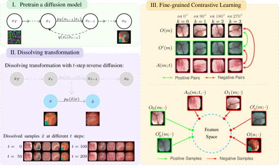
Figure 2: DIA on Kvasir-polyp dataset. (I) With a pretrained diffusion model, (II) the dissolving transformations of image $x$ result in $\hat{x}$. With a bigger time step $t$, $\hat{x}$ gradually loses fine-grained features. (III) Given images $m$ and $n$, we generated transformed versions $A(m;t,\cdot)$, $O(m;\cdot)$, $O^{\prime}(m;\cdot)$ for image $m$ and $A(n;t,\cdot)$, $O(n;\cdot)$, $O^{\prime}(n;\cdot)$ for image $n$ using a mixture of dissolving and other standard transformations. Then we form positive and negative pairs as described in Sec. 3.2.2. Here the two green positive samples form one positive pair. All other image pairings (between green and red or between red and red samples) form a negative pair.

3 Methodology

This section introduces DIA (Dissolving Is Amplifying), a method curated for fine-grained anomaly detection for medical imaging. DIA is a self-supervised method based on contrastive learning. DIA learns representations that can distinguish fine-grained discriminative features in medical images. First, DIA employs a dissolving strategy based on dissolving transformations (Sec. 3.1). The dissolving transformations are able to remove or deemphasize fine-grained discriminative features. Second, DIA uses the amplifying framework described in Sec. 3.2 to contrast images that have been transformed with and without dissolving transformations. We use the term amplifying framework as it amplifies the representation of fine-grained discriminative features.

3.1 Dissolving Strategy

We introduce dissolving transformations, a novel data augmentation strategy to create negative examples in a contrastive learning framework. The dissolving transformations can be achieved by a pre-trained diffusion model. The output image maintains a similar structure and appearance to the input image, but several fine-grained discriminative features unique to the input image are removed or attenuated. While the regular diffusion process starts with pure noise, we initialize the diffusion process with the input image without adding any noise. As depicted in Fig. 1, dissolving transformations gradually remove fine-grained discriminative features of various datasets (Figs. 1(b), 1(c), 1(d) and 1(e)). The effect of dissolving transformations increases with an increasing number of diffusion time steps $t$.

To recap, diffusion models consist of forward and reverse processes, and each process is performed for $T$ time steps. The forward process $q$ gradually adds noise to an image $x_{0}$ for $T$ steps to obtain a pure noise image $x_{T}$, whereas the reverse process $p$ aims at restoring the starting image $x_{0}$ from $x_{T}$. In particular, we sample an image $x_{0}\sim q(x_{0})$ from a real data distribution $q(x_{0})$, then add noise at each step $t$ with the forward diffusion process $q(x_{t}|x_{t-1})$, which can be expressed as:

$$\small q(x_{t}|x_{t-1}) =\mathcal{N}(x_{t};\sqrt{1-\beta_{t}}\cdot x_{t-1},\beta_{t}\cdot\text{I}),$$ (1)

$$q(x_{1:T}|x_{0}) =\prod_{t=1}^{T}q(x_{t}|x_{t-1}),$$ (2)

where $\beta_{t}$ represents a known variance schedule that follows $0<\beta_{1}<\beta_{2}<\cdots<\beta_{T}<1$. Afterwards, the reverse process removes noise starting at $p(x_{T})=\mathcal{N}(x_{T};0,\text{I})$ for $T$ steps. Let $\theta$ be the network parameters:

$$\small p_{\theta}(x_{t-1}|x_{t})=\mathcal{N}(x_{t-1};\mu_{\theta}(x_{t},t),\Sigma_{\theta}(x_{t},t)),$$ (3)

where $\mu_{\theta}$ and $\Sigma_{\theta}$ are the mean and variance conditioned on step number $t$.

The proposed dissolving transformations are based on Eq. 3. Instead of generating images by progressive denoising, we apply reverse diffusion in a single step directly on an input image. Essentially, we set $x_{t}=x$ in Eq. 3, where $x$ is the input image. We then compute an approximated state $x_{0}$ and denote it as $\hat{x}_{t\rightarrow 0}$ to make it clear that the equation below is parameterized by the time step $t$. By reparametrizing Eq. 3, $\hat{x}_{t\rightarrow 0}$ can be obtained by:

$$\small\hat{x}_{t\rightarrow 0}=\sqrt{\frac{1}{\bar{\alpha}_{t}}}\cdot x-\sqrt{\frac{1}{\bar{\alpha}_{t}}-1}\cdot\epsilon_{\theta}(x,t),$$ (4)

$$\bar{\alpha}_{t}:=\Pi_{s=1}^{t}\alpha_{s}\;\text{and}\;\alpha_{t}:=1-\beta_{t},$$

where $\epsilon_{\theta}$ is a function approximator (e.g. UNet) to predict the corresponding noise from $x$. Since a greater value of $t$ leads to a higher variance $\beta_{t}$, $\hat{x}_{t\rightarrow 0}$ is expected to remove more of the “noise” if $t$ is large. In our context, we do not remove “noise” but discriminative instance features. If $t$ is small, the removed discriminative instance features are more fine-grained. If $t$ is larger, larger discriminative instance features may be removed. See Fig. 1 for examples.

3.2 Amplifying Framework

We propose a novel contrastive learning framework to enhance the awareness of the fine-grained image features by integrating the proposed dissolving transformations. In particular, we aim to enforce the model to focus on fine-grained features by emphasizing the differences between images with and without dissolving transformations. Fig. 2 illustrates the proposed fine-grained feature learning method of DIA. We first present the different transformation branches in Sec. 3.2.1 and then introduce the fine-grained contrastive learning framework using our proposed feature-amplified NT-Xent loss in Sec. 3.2.2.

3.2.1 Transformation Branches

We extend the framework by Tack et al. [49] for contrastive learning-based anomaly detection. They employ two types of transformations: shifting transformations (e.g. large rotations) and non-shifting transformations (e.g. color jitter, random resized crop, and grayscale). During contrastive learning, an input image is transformed by $2K$ transformations, where each transformation is the concatenation of one shifting transformation and multiple non-shifting transformations.

We use a set $\mathcal{S}$ of $K$ different shifting transformations. This set contains only fixed (non-random) transformations and starts from the identity $I$ so that $\mathcal{S}:=\{S_{0}=I,S_{1},\dots,S_{K-1}\}$. With input image $x$, we obtain $S_{1}(x),\dots,S_{K-1}(x)$ as shifted images that strongly differ from the in-distribution samples $S_{0}(x)=x$. Each of these $K$ shifted images then passes through multiple non-shifting transformations $\in\mathcal{T}$. This yields the set of combined transformations $O:=\{O_{0},O_{1},\dots,O_{K-1}\}\;\text{and}\;O_{k}=\mathcal{T}\circ S_{k}$. With a slight abuse of notations, we use $\mathcal{T}$ as a sequence of random non-shifting transformations. This process is then repeated a second time, yielding another transformation set $\mathcal{O}^{\prime}$. We also refer to $\mathcal{O}$ and $\mathcal{O}^{\prime}$ as two augmentation branches. Each image is therefore transformed $2K$ times, $K$ times in each augmentation branch. All transformations have supposedly different randomly sampled non-shifting transformations, but $O_{i}(x)$ and $O^{\prime}_{j}(x)$ share the same shifting transformation if $i=j$.

Building on this framework, we introduce a third augmentation branch using dissolving transformations, denoted as $\mathcal{A}:=\{A_{0},\dots,A_{K-1}\}$. The dissolving transformations branch outputs transformations of the form:

$$\small{A}_{k}=\mathcal{T}\circ S_{k}\circ\mathcal{D}$$ (5)

where $\mathcal{T}$ is a sequence of random non-shifting transformations, $S_{k}$ is a shifting transformation, and $\mathcal{D}$ is a randomly sampled dissolving transformation. In summary, this yields $3K$ transformations of each image, $K$ in each of the three augmentation branches.

3.2.2 Fine-grained Contrastive Learning

The goal of contrastive learning is to transform input images into a semantically meaningful feature representation. To design a loss function for contrastive learning, we need to decide for which of the image pairs the feature representation should be made more similar (i.e. positive pairs) and for which of the image pairs the feature representation should be made more different (i.e. negative pairs).

For a single image, we have $3K$ different transformations. In addition, we have $B$ different images in a batch, yielding $3K\cdot B$ images that are considered jointly. For all possible pairs of images, they can either be a negative pair, a positive pair, or not be considered in the loss function. We relegate the explanation to an illustration in  Fig. 3. In the top left quadrant of the matrix, we can see the design choices of what constitutes a positive and a negative pair inherited from Tack et al. [49], based on the NT-Xent loss Chen et al. [9]. The region highlighted in red, is our proposed design for the new negative pairs for dissolving transformations. The purpose of these newly introduced negative pairs is to learn a representation that can better distinguish between fine-grained semantically meaningful features. The contrastive loss for each image sample can be computed as follows:

$$\ell_{i,j}=-\log\frac{\exp(\text{sim}({z}_{i},{z}_{j})/\tau)}{\sum_{k=1}^{3N}\mymathbb{1}_{k,i}\cdot(\exp(\text{sim}({z}_{i},{z}_{k}))/\tau)}$$ (6)

$$\mymathbb{1}_{k,i}=\begin{cases}0\quad i=k,\\ 1\quad otherwise,\end{cases}$$

where $N$ is the number of samples (i.e. $N=B\cdot K$), $sim(z,\hat{z})=z\cdot\hat{z}/||z||||\hat{z}||$, and $\tau$ is a temperature hyperparameter to control the penalties of negative samples.

Figure 3: Visualization of the target similarity matrix ($K=2$ with two samples in a batch). The white, blue, and lavender blocks denote the excluded, positive, and negative pairs, respectively. The red area contains the newly introduced negative pairs with dissolving transformations.

As mentioned previously, the positive pairs are selected from $O_{i}(\cdot)$ and $O^{\prime}_{j}(\cdot)$ branches only when $i=j$. The proposed feature-amplified NT-Xent loss can therefore be expressed as:

$$\mathcal{L}_{con}= \dfrac{1}{3BK}\dfrac{1}{|\{x_{+}\}|}\sum\ell_{i,j}\cdot\begin{cases}0&{\mymathbb{1}_{i,j}\in\{x_{-}\}}\\ 1&{\mymathbb{1}_{i,j}\in\{x_{+}\}}\end{cases},$$ (7)

where $\{x_{+}\}$ and $\{x_{-}\}$ denote the positive and negative pairs, and $|\{x_{+}\}|$ is the number of positive pairs. The resulting target similarity matrix is shown in Fig. 3.

Additionally, an auxiliary softmax classifier $f_{\theta}$ is used to predict which shifting transformation is applied for a given input $x$, resulting in $p_{cls}(y^{S}|x)$. With the union of non-dissolving and dissolving transformed samples $\mathcal{X}_{\mathcal{S}\cup\mathcal{A}}$, the classification loss is defined as:

$$\small\mathcal{L}_{cls}=\frac{1}{3B}\frac{1}{K}\sum_{k=0}^{K-1}\sum_{\hat{x}\in\mathcal{X}_{\mathcal{S}\cup\mathcal{A}}}-\log p_{cls}(y^{S}|\hat{x}).$$ (8)

The final training loss is hereby defined as:

$$\small\mathcal{L}_{DIA}=\mathcal{L}_{con}+\gamma\cdot\mathcal{L}_{cls},$$ (9)

where $\gamma$ is set to 1 in this work.

3.3 The Score functions

During inference, we adopt an anomaly score function that consists of two parts, (1) $s_{con}$ sums the anomaly scores over all shifted transformations, in addition to (2) $s_{cls}$ sums the confidence of the shifting transformation classifier. For the $k^{th}$ shifting transformation, given an input image $x$, training example set $\{x_{m}\}$, and a feature extractor $c$, we have:

$$\small s_{con}(\tilde{x},\{\tilde{x}_{m}\})=\max_{m}\;\text{sim}(c(\tilde{x}_{m}),c(\tilde{x}))\cdot||c(\tilde{x})||,$$ (10)

$$s_{cls}(\tilde{x})=W_{k}f_{\theta}(\tilde{x}),$$

$$\text{With}\quad\tilde{x}=T_{k}(x)\quad\tilde{x}_{m}=T_{k}(x_{m})$$

where $\max_{m}\text{sim}(c(x_{m}),c(x))$ computes the cosine similarity between $x$ and its nearest training sample in $\{x_{m}\}$, $f_{\theta}$ is an auxiliary classifier that aims at determining if $x$ is a shifted example or not, and $W_{k}$ is the weight vector in the linear layer of $p_{cls}(y^{S}|x)$. In practice, with $M$ training samples, balancing terms $\lambda^{S}_{con}=M/\sum_{m}s^{S}_{con}$ and $\lambda^{S}_{cls}=M/\sum_{m}s^{S}_{cls}$ are applied to scale the scores of each shifting transformation $S$. Those balancing terms slightly improve the detection performances, as reported in [49].

4 Experiments

4.1 Experiment Setting

We evaluated our methods on six datasets with various imaging protocols (e.g. CT, OCT, endoscopy, retinal fundus) and areas (e.g. chest, breast, colon, eye). In particular, we experiment on low-resolution datasets of Pnuemonia MNIST and Breast MNIST, and higher resolution datasets of SARS-COV-2, Kvasir-Polyp, Retinal-OCT, and APTOS-2019. A detailed description is in Appendix A.

We performed semi-supervised anomaly detection that uses only the normal class for training, namely, the healthy samples. Then we output the anomaly scores for each data instance to evaluate the anomaly detection performance. We use the area under the receiver operating characteristic curve (AUROC) as the metric. All the presented values are computed by averaging at least three runs.

We use ResNet18 as the backbone model and a batch size of 32. In terms of shifting transformations, we adopted rotation as suggested by CSI [49], with a fixed $K=4$ for $0\degree$, $90\degree$, $180\degree$, $270\degree$. For dissolving transformations, all diffusion models are trained on $32\times 32$ images. The diffusion step $t$ is randomly sampled from $t\sim U(100,200)$ for Kvasir-Polyp and $t\sim U(30,130)$ for the other datasets. For high-resolution datasets, we downsampled images to $32\times 32$ for feature dissolving and then resized them back, avoiding massive computations of diffusion models.

4.2 Technical Details

Our experiments are carried on NVIDIA A100 GPU server with CUDA 11.3 and PyTorch 1.11.0. We use a popular diffusion model implementation to train diffusion models for dissolving transformation, and the codebase for DIA is based on the official CSI [49] implementation. Additionally, we use the official implementation for all benchmark models included in the paper.

The Training of Diffusion Models. The diffusion models are trained with a 0.00008 learning rate, 2 step gradient accumulation, 0.995 exponential moving average decay for 25,000 steps. Each step adopts 256, 128, 32 batchsize for the resolution of $32\times 32$, $64\times 64$, $128\times 128$, respectively. Adam [28] optimizer and L1 loss are used for optimizing the diffusion model weights, and random horizontal flip is the only augmentation used. Notably, we found that automatic mixed precision [31] cannot be used for training as it impedes the model from convergence. Commonly, the models trained for around 12,500 steps are already usable for dissolving features and training DIA.

The Training of DIA. The DIA models are trained with a 0.001 learning rate with cosine annealing [29] scheduler, and LARS [56] optimizer is adopted for optimizing the DIA model parameters. After sampling positive and negative samples, dissolving transformation applies then we perform data augmentation from SimCLR [9]. We randomly select 200 samples from the dataset for training each epoch and we commonly obtain the best model within 200 epochs.

4.3 Results

We evaluate our method on six datasets, and the details for each dataset are described in Appendix A. As shown in Tab. 1, our method beats all other methods on four out of six datasets. RD4AD has the best performance on two datasets. In addition, we can significantly outperform the baseline CSI on all datasets thereby clearly demonstrating the value of our novel components.

Methods	Pnuemonia MNIST	Breast MNIST	SARS-COV-2	Kvasir-Polyp	Retinal-OCT	APTOS-2019
KDAD [43]                  (CVPR 21)	0.378$\pm$0.02	0.611$\pm$0.02	0.770$\pm$0.01	0.775$\pm$0.01	0.801$\pm$0.00	0.631$\pm$0.01
†Transformly [16] (CVPR 22)	0.821$\pm$0.01	0.738$\pm$0.04	0.711$\pm$0.00	0.568$\pm$0.00	0.824$\pm$0.01	0.616$\pm$0.01
RD4AD [17] (CVPR 22)	0.815$\pm$0.01	0.759$\pm$0.02	0.842$\pm$0.00	0.757$\pm$0.01	0.996$\pm$0.00	0.921$\pm$0.00
‡UniAD [57] (NeurIPS 22)	0.734$\pm$0.02	0.624$\pm$0.01	0.636$\pm$0.00	0.724$\pm$0.03	0.921$\pm$0.01	0.874$\pm$0.00
Meanshift [39] (AAAI 23)	0.818$\pm$0.02	0.648$\pm$0.01	0.767$\pm$0.03	0.694$\pm$0.05	0.438$\pm$0.01	0.826$\pm$0.01
Baseline CSI [49] (NeurIPS 20)	0.834$\pm$0.03	0.546$\pm$0.03	0.785$\pm$0.02	0.609$\pm$0.03	0.803$\pm$0.00	0.927$\pm$0.00
Ours                DIA	0.903$\pm$0.01	0.750$\pm$0.03	0.851$\pm$0.03	0.860$\pm$0.04	0.944$\pm$0.00	0.934$\pm$0.00
†Transformaly is trained under unimodel settings as the original paper.
‡UniAD does not support $32\times 32$ resolution. PnuemoniaMNIST and BreastMNIST datasets are trained with $128\times 128$ resolution.

Table 1: Semi-supervised fine-grained medical anomaly detection results.

5 Ablation Studies

This section presents a series of ablation studies to understand how our proposed method works under different configurations and parameter settings. In addition, we present results with heuristic blurring methods in Appendix B, along with the different designs of similarity matrix and non-medical datasets provided in Sec. C.2.

5.1 Dissolving Transformation Steps

We randomly sample dissolving step $t$ from a uniform distribution $U(a,b)$. This experiment investigates various sampling ranges. We establish the minimum step at 30 to ensure minimal changes to the image and assess effectiveness over a 100-step interval. As indicated in Tab. 2, lower steps generally yield better results. We believe the lower step dissolves fine-grained features without significantly altering the overall image appearance, as illustrated in Fig. 1. Kvasir dataset involves polyps as anomalies, which are pronounced (in the pixel space) compared to the anomalies in other datasets. Consequently, a slightly higher $t$ can lead to enhanced performance.

Step Range	SARS- COV-2	Kvasir Polyp	Retinal OCT	APTOS 2019
(  30, 130)	0.851	0.796	0.919	0.934
(130, 230)	0.827	0.860	0.895	0.920
(230, 330)	0.790	0.775	0.908	0.923
(330, 430)	0.815	0.763	0.896	0.926
(430, 530)	0.803	0.615	0.905	0.926

Table 2: Results for diffusion step range.

5.2 The Role of Diffusion Models

Given the challenges of acquiring additional medical data, we evaluate how diffusion models affect anomaly detection performances. Specifically, we limit the training data ratio ($\gamma$) for diffusion models to simulate less optimal diffusion models, while keeping other settings unchanged. This experiment examines how anomaly detection performances are impacted when deployed with underperforming diffusion models with insufficient training data.

Datasets	DIA($\gamma=0.1$)	DIA($\gamma=1$)
PneumoniaMNIST	0.745	0.903
Kvasir-Polyp	0.679	0.860

Table 3: Results with different training data ratios.

We evaluate on two small datasets where 5856 images are in PneumoniaMNIST and 8000 images are in Kvasir-Polyp. As shown in Tab. 3, a significant performance drop happened. Thus, with better trained diffusion models, better performances of anomaly detection can be obtained.

(a) Input

(b) $C,t\!=\!200$

(c) $M,t\!=\!200$

(d) $C,t\!=\!400$

(e) $F,t\!=\!400$

Figure 4: Dissolving Transformations using different diffusion models. $C$ and $M$ denote if the dissolving transformation is performed based on the diffusion models trained on CIFAR10 or the corresponding dataset, respectively.

A natural next question is, can one utilize well-trained diffusion models to perform dissolving transformations on non-training domains? A well-trained diffusion model is attuned to the attributes of its training dataset. Consequently, it may incorrectly dissolve features if the presented image deviates from the training set. Figure 4 presents the different dissolving effects using diffusion models trained on different datasets. The visual evidence suggests that a data-specific diffusion model accurately dissolves the correct instance-specific features and attempts to revert images towards a more generalized form characteristic of the dataset. In contrast, a diffusion model trained on the CIFAR dataset tends to dissolve the image in a chaotic manner, failing to maintain the image’s inherent shape.

5.3 Rotate vs. Perm

Rotate and perm (i.e. jigsaw transformation) are reported as the most performant shifting transformations [49]. This experiment evaluates their performances under fine-grained settings. As shown in Tab. 4, the rotation transformation outperforms the perm transformation.

Method	SARS-COV-2	Kvasir-Polyp	Retinal-OCT	APTOS-2019
DIA-Perm	0.841$\pm$0.01	0.840$\pm$0.01	0.890$\pm$0.02	0.926$\pm$0.00
DIA-Rotate	0.851$\pm$0.03	0.860$\pm$0.03	0.944$\pm$0.01	0.934$\pm$0.00

Table 4: Using rotate or perm for shifting transformation.

Compared to perm, rotation transforms images in a consistent manner, easing the categorization difficulties associated with the correct shifting distributions.

5.4 The Resolution of Feature Dissolved Samples

This work adopted feature-dissolved samples with a resolution of 32$\times$32, which significantly improves the anomaly detection performances. Notably, the downsample-upsample routine also dissolves fine-grained features. This experiment investigates the effects of different resolutions for feature-dissolved samples. As shown in Tab. 5 and Tab. 6, the computational cost increases dramatically with increased resolutions, while it can hardly boost model performances.

Dslv. Size	SARS-COV-2	Kvasir-Polyp	Retinal-OCT	APTOS-2019
32	0.851$\pm$0.03	0.860$\pm$0.04	0.944$\pm$0.01	0.934$\pm$0.00
64	0.803$\pm$0.01	0.721$\pm$0.01	0.922$\pm$0.00	0.937$\pm$0.00
128	0.807$\pm$0.02	0.730$\pm$0.02	0.930$\pm$0.00	0.905$\pm$0.00

Table 5: Different resolutions for dissolving transformations.

Res.	w/o	32$\times$32	64$\times$64	128$\times$128
Params (M)	11.2	19.93	19.93	19.93
MACs (G)	1.82	2.33	3.84	9.90

Table 6: Multiply–accumulate operations (MACs) for different resolutions of dissolving transformations. w/o denotes no dissolving transformation applied.

The variations in performance across different resolutions are attributed to two main factors. Firstly, the size of training samples impacts this. In larger datasets such as APTOS and Retinal-OCT, the performance degradation is less pronounced. This is because higher-resolution diffusion models require more training data. Secondly, the nature of critical features plays a role. High-resolution images naturally contain more details. In datasets like APTOS, where disease indicators are subtler in pixel space (e.g. hemorrhages or thinner blood vessels), the performance drop is minimal. In fact, 64x64 resolution images even outperform 32x32 ones for APTOS. Conversely, in datasets like Retinal-OCT, where crucial features are more prominent in pixel space (e.g. edemas), lower-resolution images help the model concentrate on these more apparent features. Notably, the computational cost of higher-resolution dissolving transformations is dramatically increased. Our results indicate that a resolution of 32x32 strikes an optimal performance for dissolving transformations and computational efficiency.

6 Discussion

Diffusion models work by gradually adding noise to an image over several steps, and then a UNet is employed to learn to reverse this process. During the training of diffusion models, the UNet learns to predict the noise that was added at each step of the diffusion process. This process indirectly teaches the UNet about the underlying structure and characteristics of the data in the dataset. Essentially, the proposed dissolving transformation executes a standalone reverse diffusion to reverse the “noise” on non-noisy input images directly. Notably, it still operates under the assumption that there is noise to be removed. Consequently, it interprets the instance-specific fine details and textures of the non-noisy image as noise and attempts to remove them (which we refer to as “dissolve” in our context), as illustrated in Fig. 1. With non-noisy input images from a non-training domain, the diffusion model fails to interpret the correct instance-specific fine details and, therefore, fails to remove the correct features inside the image, as illustrated in Fig. 4. We show additional qualitative results in the accompanying video.

Medical image data is particularly suitable for the proposed dissolving transformations. Different from other data domains, medical images typically feature a consistent prior onto which more detailed, instance-specific features are superimposed. For instance, chest X-ray images generally have a gray chest shape on a black background, with additional instance-specific features like bones, tumors, or other pathological findings, being superimposed on top. Those instance-specific features are interpreted by the UNet as “noise” and then be removed by the reverse diffusion process. By tuning the hyperparameter $t$, this process allows for the gradual removal of the most instance-specific features, moving towards making the output image look more generic. Those removed features typically contain pivotal pathological findings, which are critical for medical image analysis. Therefore, in order to amplify these removed critical features, we deploy a contrastive learning scheme to contrast a given input image and its feature-dissolved counterpart.

7 Conclusion

We proposed an intuitive dissolving is amplifying (DIA) method to support fine-grained discriminative feature learning for medical anomaly detection. Specifically, we introduced dissolving transformations that can be achieved with a pre-trained diffusion model. We use contrastive learning to enhance the difference between images that have been transformed by dissolving transformations and images that have not. Experiments show DIA significantly boosts performance on fine-grained medical anomaly detection without prior knowledge of anomalous features. One limitation is that our method requires training on diffusion models for each of the datasets. In future work, we would like to extend our method to enhance supervised contrastive learning and fine-grained classification by leveraging the fine-grained feature learning strategy.

Supplementary Material

(a) Gaussian ($k$=3)

(b) Gaussian ($k$=7)

(c) Gaussian ($k$=11)

(d) Median ($k$=3)

(e) Median ($k$=7)

(f) Median ($k$=11)

Figure 5: Heuristic alternatives to dissolving transformations with various kernel sizes. Compared with median blur, Gaussian blur preserves more image semantics.

Appendix A Datasets

We evaluated on benchmark MedMNIST datasets [54], with image sizes of $28\times 28$:

• PneumoniaMNIST [54] consists of 5,856 pediatric chest X-Ray images (pneumonia vs. normal), with a ratio of 9 : 1 for training and validation set.

• BreastMNIST [54] consists 780 breast ultrasound images (normal and benign tumor vs. malignant tumor), with a ratio of 7 : 1 : 2 for train, validation and test set.

We also evaluated on multiple high-resolution datasets that are resized to $224\times 224$:

• SARS-COV-2 [3] contains 1,252 CT scans that are positive for SARS-CoV-2 infection (COVID-19) and 1,230 CT scans for patients non-infected by SARS-CoV-2.

• Kvasir-Polyp [36] consists the 8,000 endoscopic images, with a ratio of 7 : 3 for training and testing. We remapped the labels to polyp and non-polyp classes.

• Retinal OCT [6] consists 83,484 retinal optical coherence tomography (OCT) images for training, and 968 scans for testing. We remapped the diseased categories (i.e. CNV, DME, drusen) to the anomaly class.

• APTOS-2019 [4] consists 3,662 fundus images to measure the severity of diabetic retinopathy (DR), with a ratio of 7 : 3 for training and testing. We remapped the four categories (i.e. normal, mild DR, moderate DR, severe DR, proliferative DR) to normal and DR classes.

Appendix B Heuristic Alternatives To Dissolving Transformations

With the proposed dissolving transformations, the instance-level features can hereby be emphasized and further focused. Essentially, dissolving transformations use diffusion models to wipe away the discriminative instance features. In this section, we evaluate our method with naïve alternatives to dissolving transformations, namely, Gaussian blur and median blur.

B.1 Different Kernel Sizes

We evaluate different kernel sizes for each operation. A visual comparison of those methods is provided in Fig. 5. To be consistent with the diffusion feature dissolving process, the same downsampling and upsampling processes are performed for DIA-Gaussian and DIA-Median. Referring to Tab. 1, though less performant, the heuristic image filtering operations can also contribute to the fine-grained anomaly detection tasks with a significant performance boost against the baseline CSI method.

Dataset	kernel size	DIA-Gaussian	DIA-Median
pneumonia MNIST	3	0.845$\pm$0.01	0.779$\pm$0.03
	7	0.839$\pm$0.04	0.872$\pm$0.01
	11	0.856$\pm$0.02	0.678$\pm$0.07
breast MNIST	3	0.541$\pm$0.01	0.641$\pm$0.03
	7	0.653$\pm$0.03	0.689$\pm$0.01
	11	0.749$\pm$0.05	0.542$\pm$0.04
SARS- COV-2	3	0.813$\pm$0.02	0.837$\pm$0.07
	7	0.847$\pm$0.00	0.809$\pm$0.03
	11	0.802$\pm$0.01	0.793$\pm$0.02
Kvasir Polyp	3	0.629$\pm$0.03	0.526$\pm$0.02
	7	0.586$\pm$0.02	0.514$\pm$0.05
	11	0.579$\pm$0.01	0.495$\pm$0.04

Table 7: Heuristic alternatives to dissolving transformations with various kernel sizes. The blue color denotes a suboptimal performance against our proposed dissolving transformations.

Compared against the dissolving transformations, those non-parametric heuristic methods dissolve image features regardless of the generic image semantics, resulting in lower performances. In a way, dissolving transformations dissolve instance-level image features with an awareness of discriminative instance features, by learning from the dataset. We therefore believe that the diffusion models can serve as a better dissolving transformation method for fine-grained feature learning.

B.2 Rotate vs. Perm

We supplement Tab. 4 with the heuristic alternatives to dissolving transformations in this section. As shown in Tab. 8, similar to dissolving transformations, the rotation transformation mostly outperforms the perm transformation.

Dataset	transform	Gaussian	Median	Diffusion
SARS- COV-2	Perm	0.788$\pm$0.01	0.826$\pm$0.00	0.841$\pm$0.01
	Rotate	0.847$\pm$0.00	0.837$\pm$0.07	0.851$\pm$0.03
Kvasir Polyp	Perm	0.712$\pm$0.02	0.663$\pm$0.02	0.840$\pm$0.01
	Rotate	0.739$\pm$0.00	0.687$\pm$0.01	0.860$\pm$0.03
Retinal OCT	Perm	0.754$\pm$0.01	0.747$\pm$0.03	0.890$\pm$0.02
	Rotate	0.895$\pm$0.01	0.876$\pm$0.02	0.944$\pm$0.01
APTOS 2019	Perm	0.942$\pm$0.00	0.929$\pm$0.00	0.926$\pm$0.00
	Rotate	0.922$\pm$0.00	0.918$\pm$0.00	0.934$\pm$0.00

Table 8: Comparison between rotate and perm as shifting transformation.

B.3 The Resolution of Feature Dissolved Samples

We supplement Tab. 5 with heuristic alternatives to dissolving transformations in this section. As shown in Tab. 9, those heuristic alternatives are not as performant as the proposed diffusion transformation.

Dataset	size	DIA-Gaussian	DIA-Median	DIA-Diffusion
SARS- COV-2	32	0.847$\pm$0.00	0.837$\pm$0.07	0.851$\pm$0.03
	64	0.821$\pm$0.01	0.839$\pm$0.01	0.803$\pm$0.01
	128	0.838$\pm$0.00	0.848$\pm$0.00	0.807$\pm$0.02
Kvasir Polyp	32	0.629$\pm$0.03	0.526$\pm$0.02	0.860$\pm$0.04
	64	0.686$\pm$0.00	0.575$\pm$0.02	0.721$\pm$0.01
	128	0.581$\pm$0.01	0.564$\pm$0.02	0.730$\pm$0.02
Retinal OCT	32	0.895$\pm$0.01	0.876$\pm$0.02	0.944$\pm$0.01
	64	0.894$\pm$0.00	0.887$\pm$0.00	0.922$\pm$0.00
	128	0.908$\pm$0.01	0.906$\pm$0.00	0.930$\pm$0.00
APTOS 2019	32	0.922$\pm$0.00	0.918$\pm$0.00	0.934$\pm$0.00
	64	0.910$\pm$0.00	0.917$\pm$0.00	0.937$\pm$0.00
	128	0.910$\pm$0.00	0.922$\pm$0.00	0.905$\pm$0.00

Table 9: Results for different feature dissolver resolutions.

Appendix C Additional Experiments

C.1 New Negative Pairs vs. Batchsize Increment

As the newly introduced dissolving transformation branch, given the same batch size $B$, our proposed DIA takes $3K\cdot B$ samples compared to the baseline CSI that uses $2K\cdot B$ samples. In a way, DIA increases the batchsize by a factor of $1.5$. Since contrastive learning can be batchsize dependent [24, 26], we demonstrate in Tab. 10 that our performance improvement is not due to batch size. CSI with a larger batch size exhibits similar performances as the baseline CSI method, while the proposed DIA method outperformed the baselines significantly.

Datasets	CSI	CSI-1.5	DIA
PneumoniaMNIST	0.834	0.838	0.903
BreastMNIST	0.546	0.564	0.750
SARS-COV-2	0.785	0.804	0.851
Kvasir-Polyp	0.609	0.679	0.860

Table 10: Comparison between DIA and the batch size increment. CSI-1.5 represents the baseline CSI models that are trained with $1.5$ times bigger batch sizes. To be specific, CSI and DIA are trained with a batch size of 32 while CSI-1.5 used 48.

C.2 The Design of Similarity Matrix

Shifting transformations enlarge the internal distribution differences by introducing negative pairs where the views of the same image are strongly different.

(a)

(b)

Figure 6: Visual comparison between the similarity matrices ($K=2$). The white, blue, and lavender blocks denote the excluded, positive, and negative values, respectively.

With augmentation branches $O_{i}$ and $O^{\prime}_{j}$, the target similarity matrix for contrastive learning is therefore defined where the image pairs that share the same shift transformation as positive while other combinations as negative, as presented in Fig. 6(a). Due to the introduction of the dissolving transformation branch $A_{k}$, this ablation studies the design of the target similarity matrix of those newly introduced pairs. We further evaluate the design of Fig. 6(b), where the target similarity matrix is designed to exclude the image pairs with and without dissolving transformations applied whilst sharing the same shift transformation, when $i=k$ or $j=k$. Essentially, these pairs share the same shift transformation which should be considered as positive samples, but the $A_{k}$ branch removes features that make them appear negative. Thus, we investigate whether these contradictory samples should be considered during the contrastive learning process.

Methods	SARS- COV-2	Kvasir Polyp	Retinal OCT	APTOS 2019
Baseline CSI	0.785	0.609	0.803	0.927
Ours           DIA-(a)	0.851	0.860	0.944	0.934
Ours           DIA-(b)	0.850	0.843	0.932	0.930

Table 11: Semi-supervised fine-grained medical anomaly detection results.

As shown in Tab. 11, those designs achieve very similar performances on medical datasets. Then, we further evaluate our methods on standard anomaly detection datasets, that contain coarse-grained feature differences (i.e. Car vs. Plane) with a minimum need to discover fine-grained features. We therefore further include the following datasets:

CIFAR-10 consists of 60,000 32x32 color images in 10 equally distributed classes with 6,000 images per class, including 5,000 training images and 1,000 test images.

CIFAR-100 similar to CIFAR-10, except with 100 classes containing 600 images each. There are 500 training images and 100 testing images per class. The 100 classes in the dataset are grouped into 20 superclasses. Each image comes with a ”fine” label (the class to which it belongs) and a ”coarse” label (the superclass to which it belongs), which we use in the experiments.

Note that the corresponding diffusion models for each experiment are trained on the full CIFAR10 and CIFAR100 datasets, respectively.

Dataset	Method	0	1	2	3	4	5	6	7	8	9	avg.
CIFAR10	Baseline CSI	89.9	99.1	93.1	86.4	93.9	93.2	95.1	98.7	97.9	95.5	94.3
	Ours           DIA-(a)	90.4	99.0	91.8	82.7	93.8	91.7	94.7	98.4	97.2	95.6	93.5
	Ours           DIA-(b)	80.0	98.9	80.1	74.0	81.2	84.4	82.7	94.7	93.9	89.7	86.0
Dataset	Method	0	1	2	3	4	5	6	7	8	9
CIFAR100	Baseline CSI	86.3	84.8	88.9	85.7	93.7	81.9	91.8	83.9	91.6	95.0
	Ours           DIA-(a)	85.9	82.6	87.0	84.7	91.8	84.4	92.1	79.9	90.8	95.3
	Ours           DIA-(b)	83.2	80.4	86.1	83.0	90.8	78.2	90.6	75.8	86.7	92.5
	Method	10	11	12	13	14	15	16	17	18	19	avg.
	Baseline CSI	94.0	90.1	90.3	81.5	94.4	85.6	83.0	97.5	95.9	95.2	89.6
	Ours           DIA-(a)	93.0	90.1	89.9	76.7	93.1	81.7	79.7	96.0	96.3	95.2	88.3
	Ours           DIA-(b)	91.2	86.3	87.7	73.3	91.8	80.7	79.7	97.2	95.3	93.3	86.2

Table 12: Results on standard benchmark datasets. Results are AUROC scores that are scaled by 100.

As shown in Tab. 11 and Tab. 12, the exclusion of the $i=k$ and $j=k$ pairs barely affect the performance for the fine-grained anomaly detection tasks, but significantly lowers the performance for the coarse-grained anomaly detection tasks.

Appendix D Non-Data-Specific Dissolving

As per the discussion in Secs. 5.2 and 6, we demonstrated the importance of the training for data-specific diffusion models. To further provide an intuition of what happens when using non-data-specific diffusion models, we present visual examples for the dissolving transformations with “incorrect” models. For each dataset, we show the expected dissolved images using the data-specific diffusion models (as used in our framework), dissolving with a diffusion model trained on PneumoniaMNIST dataset, dissolving with a diffusion model trained on CIFAR10 dataset, and dissolving with Stable Diffusion [40].

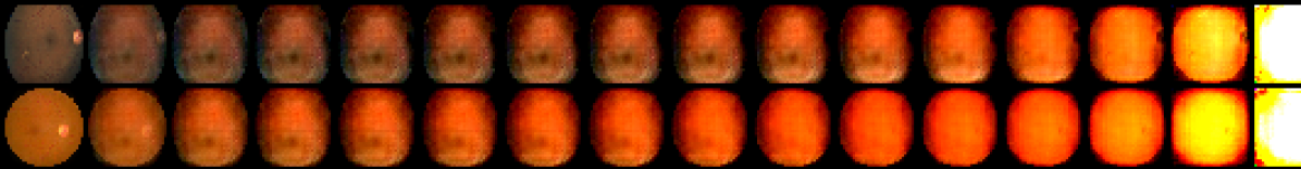
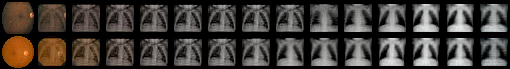
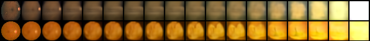
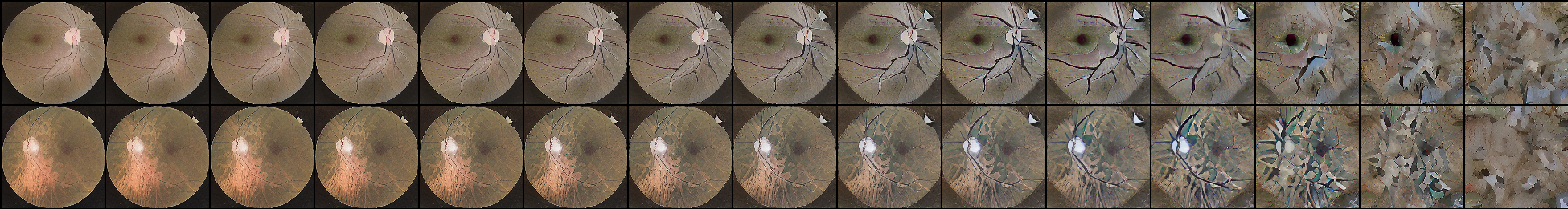
Figure 7: Visualization of APTOS dataset. From left to right are the dissolved images with increased $t$ from 1 to 975. From top to bottom, the first three rows represent models trained on the APTOS, PneumoniaMNIST, and CIFAR10 datasets, respectively. The final row showcases the output of the stable diffusion model.

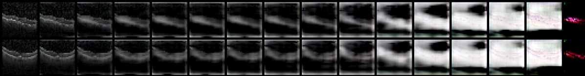
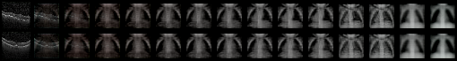
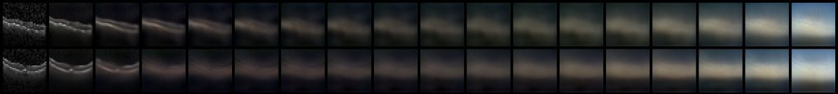
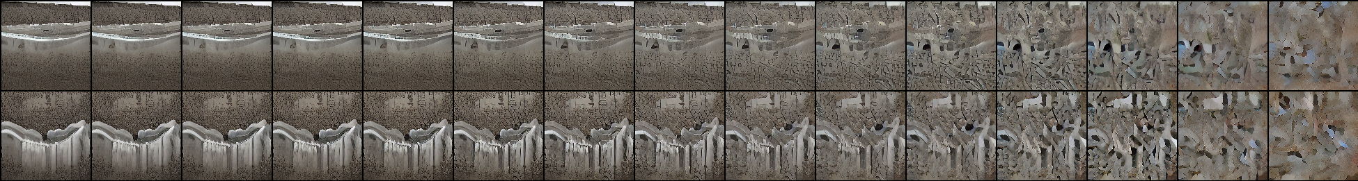
Figure 8: Visualization of OCT2017 dataset. From left to right are the dissolved images with increased $t$ from 1 to 975. From top to bottom, the first three rows represent models trained on the OCT2017, PneumoniaMNIST, and CIFAR10 datasets, respectively. The final row showcases the output of the stable diffusion model.

As illustrated in Figs. 7, 8, LABEL:fig:dslv_chestxray, 9, 10 and 11, the dissolving operation dissolves images towards the learned prior of the training dataset. Such behavior is especially significant by using the PneumoniaMNIST trained diffusion model. We can observe that all images soon look like lung x-rays, regardless of how the input looks like. For the Stable Diffusion model, the dissolving transformation removes the texture and then corrupts the image.

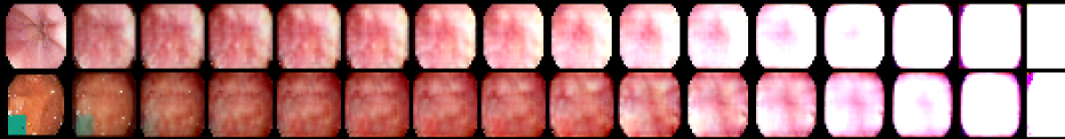
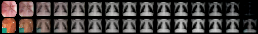
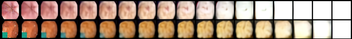
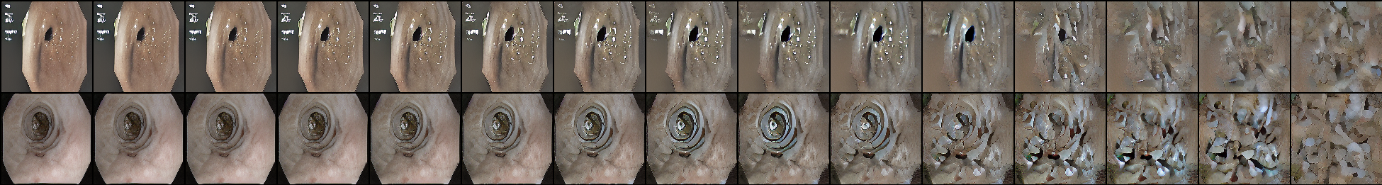
Figure 9: Visualization of Kvasir dataset. From left to right are the dissolved images with increased $t$ from 1 to 975. From top to bottom, the first three rows represent models trained on the Kvasir, PneumoniaMNIST, and CIFAR10 datasets, respectively. The final row showcases the output of the stable diffusion model.

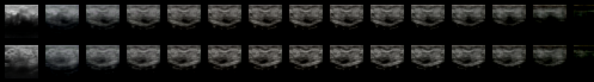
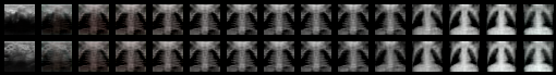
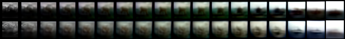
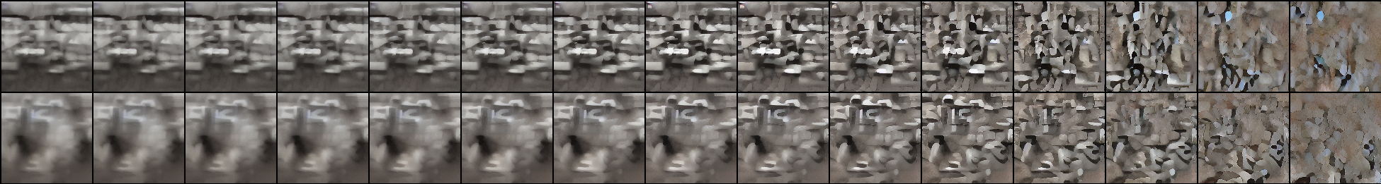
Figure 10: Visualization of BreastMNIST dataset. From left to right are the dissolved images with increased $t$ from 1 to 975. From top to bottom, the first three rows represent models trained on the BreastMNIST, PneumoniaMNIST, and CIFAR10 datasets, respectively. The final row showcases the output of the stable diffusion model.

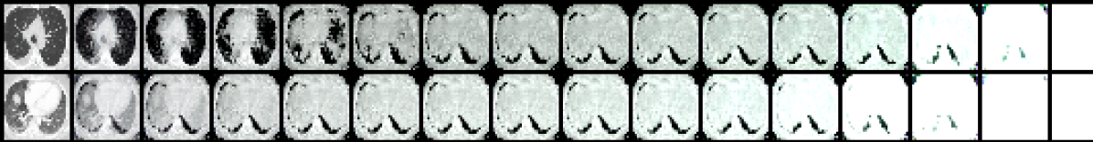
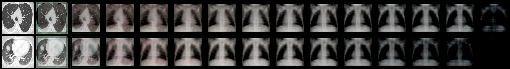
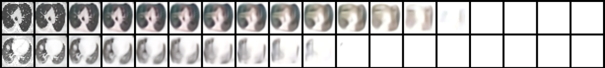
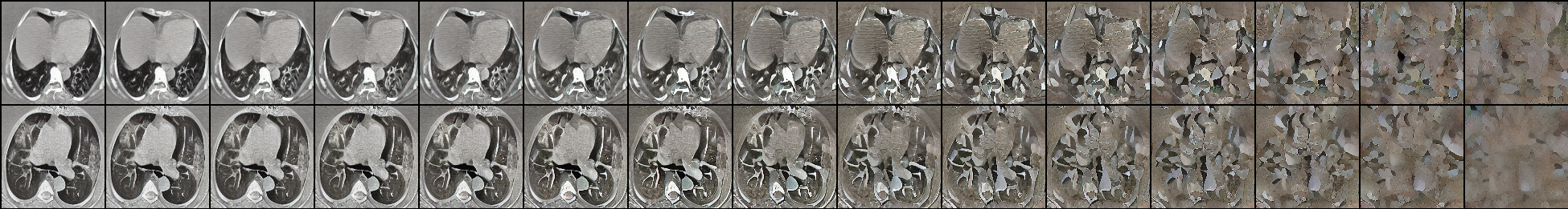
Figure 11: Visualization of SARS-COVID-2 dataset. From left to right are the dissolved images with increased $t$ from 1 to 975. From top to bottom, the first three rows represent models trained on the SARS-CoV-2, PneumoniaMNIST, and CIFAR10 datasets, respectively. The final row showcases the output of the stable diffusion model.

References

- Akcay et al. [2019a] Samet Akcay, Amir Atapour-Abarghouei, and Toby P Breckon. GANomaly: Semi-supervised anomaly detection via adversarial training. In Computer Vision – ACCV 2018, pages 622–637. Springer International Publishing, Cham, 2019a.
- Akcay et al. [2019b] Samet Akcay, Amir Atapour-Abarghouei, and Toby P Breckon. Skip-GANomaly: Skip connected and adversarially trained encoder-decoder anomaly detection. In 2019 International Joint Conference on Neural Networks (IJCNN). IEEE, 2019b.
- Angelov and Soares [2020] Plamen Angelov and Eduardo Soares. EXPLAINABLE-BY-DESIGN APPROACH FOR COVID-19 CLASSIFICATION VIA CT-SCAN. 2020.
- APTOS [2019] Asia Pacific Tele-Ophthalmology Society APTOS. Aptos 2019 blindness detection. https://www.kaggle.com/competitions/aptos2019-blindness-detection, 2019.
- Brock et al. [2018] Andrew Brock, Jeff Donahue, and Karen Simonyan. Large scale gan training for high fidelity natural image synthesis. arXiv preprint arXiv:1809.11096, 2018.
- C. Basilan et al. [2023] Ma Leticia Jose C. Basilan, https://orcid.org/0000-0003-3105-2252, Maycee Padilla, and https://orchid.org/0000-0001-5025-12872, maleticiajose.basilan@deped.gov.ph, maycee.padilla@deped.gov.ph, Department of Education- SDO Batangas Province, Batangas, Philippines. Assessment of teaching english language skills: Input to digitized activities for campus journalism advisers. International Multidisciplinary Research Journal, 4(4), 2023.
- Caron et al. [2020] Mathilde Caron, Ishan Misra, Julien Mairal, Priya Goyal, Piotr Bojanowski, and Armand Joulin. Unsupervised learning of visual features by contrasting cluster assignments. In Proceedings of Advances in Neural Information Processing Systems (NeurIPS), 2020.
- Chalapathy and Chawla [2019] Raghavendra Chalapathy and Sanjay Chawla. Deep learning for anomaly detection: A survey. arXiv preprint arXiv:1901.03407, 2019.
- Chen et al. [2020a] Ting Chen, Simon Kornblith, Mohammad Norouzi, and Geoffrey Hinton. A simple framework for contrastive learning of visual representations. In International conference on machine learning, pages 1597–1607. PMLR, 2020a.
- Chen et al. [2020b] Ting Chen, Simon Kornblith, Kevin Swersky, Mohammad Norouzi, and Geoffrey Hinton. Big self-supervised models are strong semi-supervised learners. arXiv preprint arXiv:2006.10029, 2020b.
- Chen and He [2021] Xinlei Chen and Kaiming He. Exploring simple siamese representation learning. In 2021 IEEE/CVF Conference on Computer Vision and Pattern Recognition (CVPR). IEEE, 2021.
- Chen et al. [2020c] Xinlei Chen, Haoqi Fan, Ross Girshick, and Kaiming He. Improved baselines with momentum contrastive learning. arXiv preprint arXiv:2003.04297, 2020c.
- Chen et al. [2001] Yunqiang Chen, Xiang Sean Zhou, and Thomas S Huang. One-class svm for learning in image retrieval. In Proceedings 2001 international conference on image processing (Cat. No. 01CH37205), pages 34–37. IEEE, 2001.
- Cheng et al. [2020] Haoqing Cheng, Heng Liu, Fei Gao, and Zhuo Chen. ADGAN: A scalable GAN-based architecture for image anomaly detection. In 2020 IEEE 4th Information Technology, Networking, Electronic and Automation Control Conference (ITNEC). IEEE, 2020.
- Cho et al. [2021] Hyunsoo Cho, Jinseok Seol, and Sang goo Lee. Masked contrastive learning for anomaly detection. In Proceedings of the Thirtieth International Joint Conference on Artificial Intelligence. International Joint Conferences on Artificial Intelligence Organization, 2021.
- Cohen and Avidan [2022] Matan Jacob Cohen and Shai Avidan. Transformaly - two (feature spaces) are better than one. In Proceedings of the IEEE/CVF Conference on Computer Vision and Pattern Recognition (CVPR) Workshops, pages 4060–4069, 2022.
- Deng and Li [2022] Hanqiu Deng and Xingyu Li. Anomaly detection via reverse distillation from one-class embedding. In Proceedings of the IEEE/CVF Conference on Computer Vision and Pattern Recognition (CVPR), pages 9737–9746, 2022.
- Dosovitskiy et al. [2014] Alexey Dosovitskiy, Jost Tobias Springenberg, Martin Riedmiller, and Thomas Brox. Discriminative unsupervised feature learning with convolutional neural networks. In Proceedings of the 27th International Conference on Neural Information Processing Systems - Volume 1, page 766–774, Cambridge, MA, USA, 2014. MIT Press.
- Frid-Adar et al. [2018] Maayan Frid-Adar, Idit Diamant, Eyal Klang, Michal Amitai, Jacob Goldberger, and Hayit Greenspan. Gan-based synthetic medical image augmentation for increased cnn performance in liver lesion classification. Neurocomputing, 321:321–331, 2018.
- Golan and El-Yaniv [2018] Izhak Golan and Ran El-Yaniv. Deep anomaly detection using geometric transformations. In Proceedings of Advances in Neural Information Processing Systems (NeurIPS), 2018.
- Goldstein and Dengel [2012] Markus Goldstein and Andreas Dengel. Histogram-based outlier score (hbos): A fast unsupervised anomaly detection algorithm. KI-2012: poster and demo track, 1:59–63, 2012.
- Goodfellow et al. [2014] Ian Goodfellow, Jean Pouget-Abadie, Mehdi Mirza, Bing Xu, David Warde-Farley, Sherjil Ozair, Aaron Courville, and Yoshua Bengio. Generative adversarial nets. In Advances in Neural Information Processing Systems. Curran Associates, Inc., 2014.
- Grill et al. [2020] Jean-Bastien Grill, Florian Strub, Florent Altché, Corentin Tallec, Pierre H. Richemond, Elena Buchatskaya, Carl Doersch, Bernardo Avila Pires, Zhaohan Daniel Guo, Mohammad Gheshlaghi Azar, Bilal Piot, Koray Kavukcuoglu, Rémi Munos, and Michal Valko. Bootstrap your own latent: A new approach to self-supervised learning, 2020.
- Gutmann and Hyvärinen [2012] Michael U Gutmann and Aapo Hyvärinen. Noise-contrastive estimation of unnormalized statistical models, with applications to natural image statistics. Journal of machine learning research, 13(2), 2012.
- Han et al. [2018] Changhee Han, Hideaki Hayashi, Leonardo Rundo, Ryosuke Araki, Wataru Shimoda, Shinichi Muramatsu, Yujiro Furukawa, Giancarlo Mauri, and Hideki Nakayama. Gan-based synthetic brain mr image generation. In 2018 IEEE 15th international symposium on biomedical imaging (ISBI 2018), pages 734–738. IEEE, 2018.
- He et al. [2019] Kaiming He, Haoqi Fan, Yuxin Wu, Saining Xie, and Ross Girshick. Momentum contrast for unsupervised visual representation learning. arXiv preprint arXiv:1911.05722, 2019.
- Ker et al. [2017] Justin Ker, Lipo Wang, Jai Rao, and Tchoyoson Lim. Deep learning applications in medical image analysis. Ieee Access, 6:9375–9389, 2017.
- Kingma and Ba [2014] Diederik P Kingma and Jimmy Ba. Adam: A method for stochastic optimization. arXiv preprint arXiv:1412.6980, 2014.
- Loshchilov and Hutter [2016] Ilya Loshchilov and Frank Hutter. Sgdr: Stochastic gradient descent with warm restarts. arXiv preprint arXiv:1608.03983, 2016.
- Makhzani et al. [2016] Alireza Makhzani, Jonathon Shlens, Navdeep Jaitly, Ian Goodfellow, and Brendan Frey. Adversarial autoencoders. In International Conference on Learning Representations, 2016.
- Micikevicius et al. [2017] Paulius Micikevicius, Sharan Narang, Jonah Alben, Gregory Diamos, Erich Elsen, David Garcia, Boris Ginsburg, Michael Houston, Oleksii Kuchaiev, Ganesh Venkatesh, et al. Mixed precision training. arXiv preprint arXiv:1710.03740, 2017.
- Murase and Fukumizu [2022] Hironori Murase and Kenji Fukumizu. Algan: Anomaly detection by generating pseudo anomalous data via latent variables. IEEE Access, 10:44259–44270, 2022.
- Musa and Bouras [2021] Tahani Hussein Abu Musa and Abdelaziz Bouras. Anomaly detection: A survey. In Proceedings of Sixth International Congress on Information and Communication Technology, pages 391–401. Springer Singapore, 2021.
- Pang et al. [2019] Guansong Pang, Chunhua Shen, Huidong Jin, and Anton van den Hengel. Deep weakly-supervised anomaly detection, 2019.
- Pang et al. [2021] Guansong Pang, Chunhua Shen, Longbing Cao, and Anton Van Den Hengel. Deep learning for anomaly detection. ACM Comput. Surv., 54(2):1–38, 2021.
- Pogorelov et al. [2017] Konstantin Pogorelov, Kristin Ranheim Randel, Carsten Griwodz, Sigrun Losada Eskeland, Thomas de Lange, Dag Johansen, Concetto Spampinato, Duc-Tien Dang-Nguyen, Mathias Lux, Peter Thelin Schmidt, Michael Riegler, and Pål Halvorsen. Kvasir: A multi-class image dataset for computer aided gastrointestinal disease detection. In Proceedings of the 8th ACM on Multimedia Systems Conference (MMSYS), pages 164–169, 2017.
- Pourreza et al. [2021] Masoud Pourreza, Bahram Mohammadi, Mostafa Khaki, Samir Bouindour, Hichem Snoussi, and Mohammad Sabokrou. G2d: generate to detect anomaly. In Proceedings of the IEEE/CVF Winter Conference on Applications of Computer Vision, pages 2003–2012, 2021.
- Rani and E [2020] B. Joyce Beula Rani and L. Sumathi M. E. Survey on applying GAN for anomaly detection. In 2020 International Conference on Computer Communication and Informatics (ICCCI). IEEE, 2020.
- Reiss and Hoshen [2021] Tal Reiss and Yedid Hoshen. Mean-shifted contrastive loss for anomaly detection. arXiv preprint arXiv:2106.03844, 2021.
- Rombach et al. [2021] Robin Rombach, Andreas Blattmann, Dominik Lorenz, Patrick Esser, and Björn Ommer. High-resolution image synthesis with latent diffusion models, 2021.
- Ruff et al. [2018] Lukas Ruff, Robert A. Vandermeulen, Nico Görnitz, Lucas Deecke, Shoaib A. Siddiqui, Alexander Binder, Emmanuel Müller, and Marius Kloft. Deep one-class classification. In Proceedings of the 35th International Conference on Machine Learning, pages 4393–4402, 2018.
- Sabokrou et al. [2018] Mohammad Sabokrou, Mohammad Khalooei, Mahmood Fathy, and Ehsan Adeli. Adversarially learned one-class classifier for novelty detection. In Proceedings of the IEEE Conference on Computer Vision and Pattern Recognition, pages 3379–3388, 2018.
- Salehi et al. [2021] Mohammadreza Salehi, Niousha Sadjadi, Soroosh Baselizadeh, Mohammad H Rohban, and Hamid R Rabiee. Multiresolution knowledge distillation for anomaly detection. In Proceedings of the IEEE/CVF conference on computer vision and pattern recognition, pages 14902–14912, 2021.
- Salehinejad et al. [2018] Hojjat Salehinejad, Shahrokh Valaee, Tim Dowdell, Errol Colak, and Joseph Barfett. Generalization of deep neural networks for chest pathology classification in x-rays using generative adversarial networks. In 2018 IEEE international conference on acoustics, speech and signal processing (ICASSP), pages 990–994. IEEE, 2018.
- Salem et al. [2018] Milad Salem, Shayan Taheri, and Jiann Shiun Yuan. Anomaly generation using generative adversarial networks in host-based intrusion detection. In 2018 9th IEEE Annual Ubiquitous Computing, Electronics & Mobile Communication Conference (UEMCON), pages 683–687. IEEE, 2018.
- Schlegl et al. [2017a] Thomas Schlegl, Philipp Seeböck, Sebastian M Waldstein, Ursula Schmidt-Erfurth, and Georg Langs. Unsupervised anomaly detection with generative adversarial networks to guide marker discovery. In Lecture Notes in Computer Science, pages 146–157. Springer International Publishing, Cham, 2017a.
- Schlegl et al. [2017b] Thomas Schlegl, Philipp Seeböck, Sebastian M. Waldstein, Ursula Schmidt-Erfurth, and Georg Langs. Unsupervised anomaly detection with generative adversarial networks to guide marker discovery, 2017b.
- Shekarizadeh et al. [2022] Soroor Shekarizadeh, Razieh Rastgoo, Saif Al-Kuwari, and Mohammad Sabokrou. Deep-disaster: Unsupervised disaster detection and localization using visual data, 2022.
- Tack et al. [2020] Jihoon Tack, Sangwoo Mo, Jongheon Jeong, and Jinwoo Shin. Csi: Novelty detection via contrastive learning on distributionally shifted instances. Advances in neural information processing systems, 33:11839–11852, 2020.
- Thudumu et al. [2020] Srikanth Thudumu, Philip Branch, Jiong Jin, and Jugdutt Jack Singh. A comprehensive survey of anomaly detection techniques for high dimensional big data. Journal of Big Data, 7(1):1–30, 2020.
- Wen et al. [2016] Yandong Wen, Kaipeng Zhang, Zhifeng Li, and Yu Qiao. A discriminative feature learning approach for deep face recognition. In European conference on computer vision, pages 499–515. Springer, 2016.
- Williams et al. [2002] Graham Williams, Rohan Baxter, Hongxing He, Simon Hawkins, and Lifang Gu. A comparative study of rnn for outlier detection in data mining. In 2002 IEEE International Conference on Data Mining, 2002. Proceedings., pages 709–712. IEEE, 2002.
- Wyatt et al. [2022] Julian Wyatt, Adam Leach, Sebastian M. Schmon, and Chris G. Willcocks. Anoddpm: Anomaly detection with denoising diffusion probabilistic models using simplex noise. In Proceedings of the IEEE/CVF Conference on Computer Vision and Pattern Recognition (CVPR) Workshops, pages 650–656, 2022.
- Yang et al. [2021] Jiancheng Yang, Rui Shi, Donglai Wei, Zequan Liu, Lin Zhao, Bilian Ke, Hanspeter Pfister, and Bingbing Ni. Medmnist v2: A large-scale lightweight benchmark for 2d and 3d biomedical image classification. arXiv preprint arXiv:2110.14795, 2021.
- Ye et al. [2022] Fei Ye, Chaoqin Huang, Jinkun Cao, Maosen Li, Ya Zhang, and Cewu Lu. Attribute restoration framework for anomaly detection. IEEE Transactions on Multimedia, 24:116–127, 2022.
- You et al. [2017] Yang You, Igor Gitman, and Boris Ginsburg. Large batch training of convolutional networks. arXiv preprint arXiv:1708.03888, 2017.
- You et al. [2022] Zhiyuan You, Lei Cui, Yujun Shen, Kai Yang, Xin Lu, Yu Zheng, and Xinyi Le. A unified model for multi-class anomaly detection. In Proceedings of Advances in Neural Information Processing Systems (NeurIPS), 2022.
- Zhang et al. [2021] Yuxuan Zhang, Huan Ling, Jun Gao, Kangxue Yin, Jean-Francois Lafleche, Adela Barriuso, Antonio Torralba, and Sanja Fidler. Datasetgan: Efficient labeled data factory with minimal human effort. In CVPR, 2021.
- Zhao et al. [2018] Zhixuan Zhao, Bo Li, Rong Dong, and Peng Zhao. A surface defect detection method based on positive samples. In Lecture Notes in Computer Science, pages 473–481. Springer International Publishing, 2018.