Massively Parallel Computation in a Heterogeneous Regime

Abstract

Massively-parallel graph algorithms have received extensive attention over the past decade, with research focusing on three memory regimes: the superlinear regime, the near-linear regime, and the sublinear regime. The sublinear regime is the most desirable in practice, but conditional hardness results point towards its limitations.

In this work we study a heterogeneous model, where the memory of the machines varies in size. We focus mostly on the heterogeneous setting created by adding a single near-linear machine to the sublinear MPC regime, and show that even a single large machine suffices to circumvent most of the conditional hardness results for the sublinear regime: for graphs with $n$ vertices and $m$ edges, we give (a) an MST algorithm that runs in $O(\log\log(m/n))$ rounds; (b) an algorithm that constructs an $O(k)$-spanner of size $O(n^{1+1/k})$ in $O(1)$ rounds; and (c) a maximal-matching algorithm that runs in $O(\sqrt{\log(m/n)}\log\log(m/n))$ rounds. We also observe that the best known near-linear MPC algorithms for several other graph problems which are conjectured to be hard in the sublinear regime (minimum cut, maximal independent set, and vertex coloring) can easily be transformed to work in the heterogeneous MPC model with a single near-linear machine, while retaining their original round complexity in the near-linear regime. If the large machine is allowed to have superlinear memory, all of the problems above can be solved in $O(1)$ rounds.

1 Introduction

The massively-parallel computation (MPC) model was introduced in [41] as a theoretical model of the popular Map-Reduce framework and other types of large-scale parallel computation, and has received significant attention from the distributed computing and algorithms communities. In the MPC model we have $K$ machines, each with a local memory of size $s$, operating on an input of size $N$ that is initially distributed arbitrarily across the machines. It is typically (but not always) assumed that $K\cdot s=\tilde{O}(N)$, so that the total amount of memory in the system is of the same order as the input size. All machines can communicate directly with one another; the computation proceeds in synchronous rounds, with each machine sending and receiving at most $s$ bits in total per round. Of particular interest in this model are graph problems, where the input is a graph $G=(V,E)$ on $n$ vertices, with the edges of the graph initially distributed arbitrarily among the machines.

The research on MPC graph algorithms typically considers three memory regimes: the superlinear regime, where the memory of each machine is $s=O(n^{1+\gamma})$ for some $\gamma\in(0,1)$; the near-linear regime, where $s=O(n\operatorname{\mathrm{polylog}}{n})$; and the sublinear regime, where $s=O(n^{\gamma})$ for some $\gamma\in(0,1)$. Many graph algorithms have been developed for the various regimes (e.g., [41, 34, 44, 4, 9, 19, 5, 11, 33, 13, 7, 30, 43, 28, 27, 16, 26, 29, 32, 31, 18, 22, 14, 10, 20, 47, 17]). The sublinear regime is the most desirable in practice: when designing a distributed server cluster, it is most economical to deploy many weak servers. However, this configuration is also the most challenging, since it does not allow a single machine to store information about all the vertices of the graph. It is conjectured that even some simple problems on sparse graphs are somewhat hard in the sublinear MPC model: the “2-vs-1 cycle” problem, where we are asked to distinguish between a graph that is a single large cycle and graphs that comprise two cycles, is conjectured to require $\Omega(\log{n})$ rounds, and based on this conjecture and a beautiful connection to local distributed algorithms, [29] establishes several conditional hardness results for sublinear MPC, and these are refined in [17] (see, e.g., [47] for an overview of more hardness results in the sublinear MPC model).

In this paper our goal is to interpolate between the various MPC regimes, and ask what can be done in a heterogeneous MPC regime where we have a small number of machines with large memories, and many machines with small memories. Compared to the larger-memory regimes (near-linear and superlinear), the heterogeneous regime is more practical; thus, our hope is to have the best of both worlds — the efficiency of the larger-memory regimes, together with the practicality and economic feasibility of the sublinear regime, with the addition of a few strong (near-linear or superlinear) servers.

The starting point for our work is the observation that the “$2$-vs-$1$ cycle” problem becomes trivial if we have even a single machine with memory $\Omega(n\log{n})$. This motivates us to ask whether the problems whose conditional hardness rests on the hardness of the “2-vs-1 cycle” problem — connectivity, minimum-weight spanning tree, maximal matching, and others — also become easy given a small number of large machines. For the sake of concreteness, since one large machine suffices to beat the “2-vs-1 cycle” problem, we focus throughout on a model where we have a single machine with memory $O(n\operatorname{\mathrm{polylog}}{n})$, and the other machines have sublinear memory, $O(n^{\gamma}\operatorname{\mathrm{polylog}}{n})$ for some $\gamma\in(0,1)$. Unless specified explicitly differently, by saying Heterogeneous MPC model we refer to this setting that consists of a single large machine. We show that indeed, for several of the problems from [29], a single large machine suffices to circumvent the conditional hardness results from the sublinear regime, and either match or come close to the complexity of these problems in the near-linear regime.

Our results

Table 1 below summarizes our results: for a graph on $n$ vertices and $m$ edges, with maximum degree $\Delta$ and diameter $D$, we compare the best known algorithms for the sublinear regime, the near-linear regime, and our results for the heterogeneous regime.

Although the heterogeneous model has not been explicitly studied in the past (to our knowledge), several algorithms that were developed for the near-linear regime easily translate to the heterogeneous regime, as they either already require only one large machine or can be easily modified to do so, and we indicate those in the table. We highlight in bold the three problems — MST, spanners, and maximal matching — for which we developed substantially different algorithms for the heterogeneous regime.

Problem	Sublinear MPC	Heterogeneous MPC	Near-linear MPC
Connectivity	$O(\log{D}+\log\log{n})$ [11]	$O(1)$ [1]	$O(1)$ [1]
MST	$O(\log{n})$ [5]	$O(\log\log(\frac{m}{n}))$ [new]	$O(1)$ [1]
$(1+\epsilon)$-approx. MST	no better result known for $(1+\epsilon)$-approx. than for exact	$O(1)$ [1]	exact in $O(1)$ [1]
$O(k)$-spanner of size $O(n^{1+1/k})$	$O(\log{k})$ [14]	$O(1)$ [new]	$O(1)$ [22]
Exact unweighted min-cut	$O(\operatorname{\mathrm{polylog}}{n})$ [25]	$O(1)$ [32]	$O(1)$ [32]
Approx. weighted min-cut	$(2+\epsilon)$-approx. in $O(\log{n}\cdot\log\log{n})$ [31]	$(1\pm\epsilon)$-approx. in $O(1)$ [31]	exact in $O(1)$ [31]
$(\Delta+1)$ vertex coloring	$O(\log\log\log{n})$ [19]	$O(1)$ [6]	$O(1)$ [6]
Maximal independent set	$O(\sqrt{\log\Delta}\cdot\log\log\Delta+\sqrt{\log\log{n}})$ [33]	$O(\log\log(\Delta))$ [26]	$O(\log\log(\Delta))$ [26]
Maximal matching	$O(\sqrt{\log\Delta}\cdot\log\log\Delta+\sqrt{\log\log{n}})$ [33]	$O(\sqrt{\log\frac{m}{n}}\log\log\frac{m}{n})$ [new]	$O(\log\log(\Delta))$ [13]

Table 1: Algorithms for fundamental graph problems in sublinear MPC, Heterogeneous MPC and near-linear MPC

These results can be further improved if the single large machine has more memory: with memory $\tilde{O}(n^{1+f(n)})$ for a function $f(n)=\Omega(1/\log{n})$, we can solve MST in $O(\log(\log(m/n)/(f(n)\log{n})))$ rounds, and the maximal matching algorithm of [44] can be used to find a maximal matching in $O(1/f(n))$ rounds. However, to go all the way down to $O(1)$ rounds, we require $f=\Omega(1)$, that is, the large machine needs to have $\Omega(n^{1+\gamma})$ memory for some constant $\gamma\in(0,1)$. It remains an intriguing open problem whether this can be improved.

Our techniques

In order to utilize the single large machine at our disposal, our algorithms for the Heterogeneous MPC model have the following flavor: first, we select a sparse subgraph $G^{\prime}$ of our input graph $G$, such that $G^{\prime}$ has only $\tilde{O}(n)$ edges; the subgraph $G^{\prime}$ is either sampled at random or obtained by working to sparsify the input graph, or both. We send $G^{\prime}$ to the large machine and have it compute some partial solution for $G$. Since the large machine sees only the subgraph $G^{\prime}$, the partial solution it finds typically induces an “over-approximation” of the true solution for $G$: for example, in the case of spanners, the partial solution found by the large machine induces a spanner with more edges than necessary. However, we prove that the induced solution is “not too large” (or, in the case of MST, use the KKT sampling lemma [40], which asserts exactly this). The large machine then encodes the partial solution in the form of a labeling, $L:V^{\prime}\rightarrow\left\{0,1\right\}^{\operatorname{\mathrm{polylog}}(n)}$, of the vertices of $G^{\prime}$, which it sends to the small machines: each small machine is given the labels of all vertices whose edges it stores. Finally, the small machines use the labels to select edges that are part of the true solution for $G$, and we somehow combine the selected edges to come up with the correct solution for $G$, either by using the large machine again or by other means.

Similar approaches of sub-sampling and over-approximation were previously used to obtain many efficient algorithms for a wide range of graph problems in different models, such as the streaming model ([1, 2]), the Congested Clique model ([35, 48, 50, 37]), the near-linear MPC model ([31, 32, 6]), and the super-linear MPC model ([44]). Although not explicitly stated in these terms, some of these results in fact require only a single large machine, or can be adapted to do so (see Table 1).

Hardness results of sublinear MPC

The connection between lower bounds in the sublinear MPC model and Boolean circuit complexity was investigated first in [51], and later on by [24]. In [51] it is shown that proving a super-constant lower bound in sublinear MPC for any problem in $\mathsf{P}$ would imply $\mathsf{NC}_{1}\subsetneq\mathsf{P}$, which suggests that any such lower bound is beyond the reach of current techniques. This has led the research community to focus more on conditional lower bounds (e.g. [29, 47, 17]). As previously discussed, the “1-vs-2 cycle” problem is conjectured to have round complexity $\Omega(\log{n})$ in sublinear MPC; this immediately implies the same lower bound for problems such as MST and shortest-paths. A general framework for lifting existing lower bounds from the distributed $\mathsf{LOCAL}$ model to obtain conditional lower bounds in sublinear MPC was given in [29], and refined and extended in [17]. The conditional lower bounds of [29, 17] include an $\Omega(\log\log{n})$ conditional lower bound for any component-stable algorithm computing a constant approximation of maximum matching, a constant approximation of vertex cover, or a maximum independent set, an $\Omega(\sqrt{\log\log{n}})$ conditional lower bound for computing $(\Delta+1)$-coloring, and an $\Omega(\log{k})$ conditional lower bound on computing an $O(k)$-spanner with $O(n^{1+1/k})$ edges.

Additional related work

Beyond the results summarized in Table 1, there are some algorithms that can achieve good dependence on graph parameters other than $n$ and $\Delta$. Of some relevance, for graphs with arboricity $\alpha$, in the sublinear regime, a maximal independent set or a maximal matching can be computed in $O(\sqrt{\log\alpha}\log\log\alpha+\log\log{n}\log\log\Delta)$ rounds [10]. The arboricity $\alpha$ of a graph satisfies $m/n\leq\alpha\leq\Delta$, so our result for the Heterogeneous MPC is quantitatively better (of course, [10] works in the sublinear regime, so no direct comparison is possible).

Another approach that extends the MPC model into a more realistic one is the Adaptive MPC model [12]. In the AMPC model, for an input of size $N$ there are $m$ machines, each with memory of size $S$, such that $m\cdot S=\tilde{O}(N)$. Additionally, there is a collection of distributed data stores, denoted by $D_{0},D_{1},...$, such that in the $i$’th round, each machine can read data from $D_{i-1}$ and write to $D_{i}$. The number of bits a machine can read and write in one round is limited by $O(S)$. As opposed to the native MPC, it is not required for a machine to read all of the $O(S)$ bits at once in the beginning of the round. Instead, each machine can query bits based on previous queries that it has already made in the same round. This adaptive behavior was the reasoning for the model name. It was claimed by [12] that the AMPC model could actually be more practical than the general MPC in many cases. Specifically, they pointed out that the MPC model does not take into consideration the ability to perform RDMA operations, by which a data stored on a remote machine can be read with only a few microsecond latency without requiring a synchronized round of communication. The AMPC model tries to close this gap between theory and practice. Indeed, this model efficiently solves a few problems which were considered hard for the native MPC model. Among them are the minimum spanning tree problem, which can be solved in $O(\log\log_{\frac{m}{n}}(n))$ rounds, and maximal independent set, which can be solved in $O(1)$ rounds.

2 Preliminaries

Graph notation

In this work we consider undirected graphs $G=(V,E)$, which may be either weighted or unweighted. We let $n$ denote the number of vertices in the graph, and $m$ the number of edges. If the graph is weighted, the weight function is given by $w:V\rightarrow\{1,\dots,\operatorname{poly}(n)\}$ (positive integer weights bounded by some fixed polynomial of $n$), and we make the standard assumption that all edge weights are unique, and can each be represented in $O(\log{n})$ bits.

For a set $S\subseteq V$ of nodes, let $E[S,V\setminus S]\subseteq E$ denote the edges that have one endpoint in $S$ and one in $V\setminus S$. Let $\operatorname{dist}_{G}(u,v)$ denote the unweighted (resp. weighted) distance between $u,v\in V$ in the unweighted (resp. weighted) graph $G$. We omit the subscript $G$ when the graph is clear from the context. We use the words “node” and “vertex” interchangeably.

The Heterogeneous MPC model

In the Heterogeneous MPC model, we have one large machine, which has memory $O(n\operatorname{\mathrm{polylog}}(n))$, and $K=m/n^{\gamma}$ small machines, each with memory $O(n^{\gamma}\operatorname{\mathrm{polylog}}(n))$, where $\gamma\in(0,1)$ is a parameter of the model. The small machines are numbered $1,\ldots,K$, and when we say predecessor, successor, or consecutive machines, we refer to this numbering. We assume that each machine has a source of private randomness (no shared randomness is assumed).

The input to the computation is a weighted or unweighted undirected graph $G=(V,E)$. The vertices $V$ of the input graph are fixed in advance, and the edges $E$ are initially stored on the small machines arbitrarily. If $G$ is weighted, then the weight function is specified by representing each edge as $(\left\{u,v\right\},w(\left\{u,v\right\}))$.

The computation proceeds in synchronous rounds, where each machine can communicate with all the other machines, subject to each machine $M$ sending and receiving in total only as many bits as it can store in its memory (i.e., no more than $O(n\operatorname{\mathrm{polylog}}{n})$ bits for the large machine, or $\tilde{O}(n^{\gamma})$ bits for the small machines). Between rounds, the machines may perform arbitrary computations on their local data, unbounded by time or by space. At the end of the computation, the output is either stored on the large machine, if the size of the output allows, or distributed across the small machines if the output is too large.

Throughout the paper, ”with high probability” means with probability $1-1/n^{d}$ for some $d\geq 1$.

Algorithmic tools

In this section we describe some general tools that can be useful in Heterogeneous MPC model and we will use throughout the paper. They rely mostly on known results for the sublinear MPC regime.

Claim 1 (Sorting [34]).

Given a set of $N$ comparable elements as input stored on the small machines, there is an $O(1)$-round algorithm that sorts the items on the small machines, such that at the end, for any two small machines $M<M^{\prime}$, each item stored on $M$ is no greater than any item stored on $M^{\prime}$.

One useful set of tools from prior work is fast aggregation or dissemination of information in sublinear MPC. We use minor variants of these techniques that also may involve the large machine.

Definition 1.

We say that $f:2^{S}\rightarrow S$ is an aggregation function if for all $k\geq 1$ and subsets $X_{1},\ldots,X_{k}\subseteq S$ we have $f(\left\{f(X_{1}),\ldots,f(X_{k})\right\})=f(X_{1}\cup\ldots\cup X_{k})$.

Let $\mathbb{N}^{S}$ denote the set of all multisets whose elements are drawn from $S$.

Claim 2 (Aggregation [7, 21]).

Fix a domain $S$, partitioned into predetermined subsets $S_{1},\ldots,S_{t}$, known in advance to all machines, and let $f:\mathbb{N}^{S}\rightarrow S$ be an aggregation function that is fixed in advance and known to all machines. We assume that the elements of $S$ can be represented in $O(\operatorname{\mathrm{polylog}}{n})$ bits. Let $A\subseteq S$ be a set or a multiset stored on the small machines, and let $A_{i}=A\cap S_{i}$. Then there is a constant-round algorithm that computes $f(A_{1}),\ldots,f(A_{t})$, such that at the end of the algorithm, for each $i$, the value $f(A_{i})$ is known to some small machine $M_{i}$ that is fixed in advance.

Claim 3 (Dissemination [7, 21]).

Fix a domain $S$, partitioned into predetermined subsets $S_{1},\ldots,S_{t}$ which are known to all machines, and let $A\subseteq S$ be stored on the small machines. Let $A_{i}=A\cap S_{i}$. Suppose the large machine holds values $x_{1},\ldots,x_{t}\in\left\{0,1\right\}^{(\operatorname{\mathrm{polylog}}{n})}$. There is a constant-round algorithm that disseminates $x_{i}$ to every small machine that stores an element from $A_{i}$, in parallel for all $i=1,\ldots,t$.

Proof of Claims 2 and 3..

For concreteness we focus on the context of graph problems and assume that for all $1\leq i\leq t$, the set $A_{i}$ is associated with some node $u\in V$. These assumptions hold in all the places we use Claim 2 and 3 through out the paper, but we note that the claim can be proved without them.

First, for each edge $(u,v)\in E$ we make two directed copies, $(u,v)$ and $(v,u)$. We sort all directed edges on the small machines in lexicographic order. Let $M_{u}$ be the first machine that stores some outgoing edges of vertex $u$. Each small machine $M$ sends to its successor the largest vertex $u$ such that some edge $(u,v)$ is stored on $M$. If $M$ holds some edge $(u,v)$ such that the predecessor of $M$ holds no outgoing edges of $u$, then $M$ informs the large machine that $M$ is the first machine that holds an outgoing edge of $u$ (i.e., $M_{u}=M$). Let $M^{\prime}_{u}$ be the last machine that holds some outgoing edge of $u$. The large machine now knows the range of machines $[M_{u},M^{\prime}_{u}]$ that hold edges adjacent to $u$, for each $u\in V$. Let $T_{u}$ be a tree with branching factor $n^{\gamma}$, rooted at $M_{u}$, whose nodes are the machines in the range $[M_{u},M_{u}^{\prime}]$, such that for any two machines $M<M^{\prime}$, the depth of $M$ (its distance from the root) is no greater than the depth of $M^{\prime}$. There are at most $n^{1-\gamma}$ machines that store outgoing edges of $u$, so the depth of $T_{u}$ is $O((1-\gamma)/\gamma)$. We fix $T_{u}$ in advance as a function of $u$, $M_{u}$, $M^{\prime}_{u}$. The large machine informs $M_{u}$ about the range $[M_{u},M^{\prime}_{u}]$. Then, the machine $M_{u}$ knows all its children in $T_{u}$ and what is the size of all its children’s sub-trees, so it sends to each of its children the size of its sub-tree. By induction, each machine $M$ in the range $[M_{u},M^{\prime}_{u}]$ that receives the size of its sub-tree from its parent in $T_{u}$, knows all its children in $T_{u}$ and what is the size of all its children’s sub-trees. So, in $O((1-\gamma)/\gamma)$ rounds all machines in the range $[M_{u},M^{\prime}_{u}]$ can know the IDs of their parent and their children in $T_{u}$. Note that $M$ can only be an inner node in one tree $T_{u}$: if $M$ is not a leaf in $T_{u}$, then there is some machine $M^{\prime}$ in $T_{u}$ whose depth is greater than $M$’s depth, meaning that $M<M^{\prime}$ and so $M$ is not the last machine that stores outgoing edges of $u$; there can be at most one node $u$ such that $M$ stores some but not all edges of $u$. Thus, each machine participates in at most one tree.

For the proof of Claim 2, we have each machine $M$ in the leaf of the tree $T_{u}$ computes $f(B_{u})$ such that $B_{u}\subseteq A_{u}$ is the set of elements that $M$ holds and send the computed value to its parent. Each inner-node machine computes $f(Y)$ such that $Y$ is the set of computed values received from all its children. The machine $M_{u}$, which is the root of $T_{u}$ will have the final result $f(A_{u})$ in $O((1-\gamma)/\gamma)$ rounds.

To prove Claim 3, we disseminate a value $x_{u}$ to the machines in $T_{u}$ by having each machine in $T_{u}$ sending $x_{u}$ to all its children, starting from the root $M_{u}$. All the machines in $T_{u}$ that hold an element from $A_{u}$ will know the value $x_{u}$ in $O((1-\gamma)/\gamma)$ rounds.

∎

Occasionally we will need to arrange the edges of a graph, so that all edges adjacent to a given node are stored on consecutive machines. For this purpose we switch to a directed version of the graph, where each edge $\left\{u,v\right\}$ appears in both orientations, $(u,v)$ and $(v,u)$. We then sort the edges by their source node:

Claim 4 (Arranging Nodes).

In $O(1)$ rounds, it is possible to arrange the edges of a directed graph $G=(V,E)$ on the small machines, such that

1. For each vertex $v\in V$, the outgoing edges of $v$ are stored on consecutive small machines.

2. For each $v\in V$, let $M_{\mathrm{first}}(v)$ be the first small machine that holds some outgoing edge of $v$. Then the large machine knows $M_{\mathrm{first}}(v)$ for each $v\in v$, and each small machine $M$ knows whether $M=M_{\mathrm{first}}(v)$ for each $v\in V$.

3. For each $v\in V$, the large machine and the small machine $M_{\mathrm{first}}(v)$ know the out-degree $\deg_{\mathrm{out}}(v)$ of $v$.

Proof of Claim 4..

We sort all the edges using Claim 1. Next, using Claim 2, we compute the degree $\deg_{\mathrm{out}}(v)$ of each node $v\in V$, using the domain $S=V\times\mathbb{N}$, the partition $\left\{S_{u}=\left\{u\right\}\times\mathbb{N}\right\}_{u\in V}$, the aggregation function $f(\left\{(u,x_{1}),\ldots,(u,x_{t})\right\})=(u,\sum_{i=1}^{t}x_{i})$, and initial multiset $A=\left\{(u,1):(u,v)\in E,u<v\right\}$. The small machines then report the node degrees to the large machines. Using this information, the large machine is able to identify the machine $M_{\mathrm{first}}(v)$ for each $v\in V$, and inform $M_{\mathrm{first}}$ itself. ∎

3 MST in $O(\log\log({m}/{n})$) Rounds

In this section we show how to compute a minimum-weight spanning tree in the Heterogeneous MPC model. Although we are mostly interested in the case where the large machine has near-linear memory, we state a more general result, which can use a large machine with memory $n^{1+f(n)}$ for any $f(n)=\Omega(1/\log{n})$:

Theorem 3.1.

Given a single machine with memory size $\tilde{\Omega}(n^{1+f(n)})$ and $\Omega(m/n^{\gamma})$ machines with memory $\tilde{\Omega}(n^{\gamma})$ (where $\gamma\in(0,1),f(n)=\Omega(1/\log{n})$), there is an algorithm that computes a minimum spanning tree with high probability in $O(\log(\log(m/n)/(f(n)\log{n})))$ rounds.

For most of the section, we focus on the case where the large machine has near-linear memory, i.e., $f(n)=1/\log{n}$. In this case the round complexity we get is $O(\log\log(m/n))$. Finally, we show how the proposed algorithm can be generalized for any $f(n)=\Omega(1/\log{n})$ to prove Theorem 3.1.

Before presenting our MST algorithm, we review the KKT sampling lemma, on which our algorithm relies.

The KKT sampling lemma [40]

The sampling lemma of Karger, Klein and Tarjan [40] was developed in the context of sequential MST computation, and has also been used in distributed MST algorithms, e.g.,  [48, 50, 35, 37]. Informally, the lemma asserts that for any graph $G$ whose MST we wish to compute, if we sample a random subgraph $H$ where each edge of $G$ is included with probability $p$, then a minimum-weight spanning forest (MSF) $F$ of $H$ can be used to dismiss from consideration all but $O(n/p)$ edges of $G$.

More formally, let $G=(V,E)$, let $H=(V,E^{\prime})$ be a subgraph of $G$, and let $F=(V,E^{\prime\prime})$ be a spanning forest of $H$. An edge $e\in E$ is called $F$-heavy if adding $e$ to the forest $F$ creates a cycle, and $e$ is the heaviest edge in that cycle. If $e$ is not $F$-heavy then we say that $e$ is $F$-light. No $F$-heavy edge can be in the MST of $G$; thus, we can restrict our attention to the $F$-light edges of $G$. The KKT sampling lemma states that the MSF of a random subgraph $H$ of $G$ suffices to significantly sparsify $G$.

Lemma 3.2 (Random-Sampling Lemma [40]).

Let $H$ be a subgraph obtained from $G$ by including each edge of $G$ independently with probability $p$, and let $F$ be the minimum spanning forest of $H$. The expected number of $F$-light edges in $G$ is at most $n/p$, where $n$ is the number of vertices of $G$.

Overview of our MST algorithm

Our MST algorithm consists of two parts: in the first part, we apply $O(\log\log(m/n))$ steps of the doubly-exponential Borůvka technique from [45], where in the $i$-th step, each remaining vertex selects its $2^{2^{i}}$ lightest outgoing edges and merges with the vertices on the other side of those edges. After $O(\log\log(m/n))$ such steps, there remain at most $n^{\prime}=n^{2}/m$ vertices. This number is small enough that we can afford to switch to a different approach and use the KKT lemma.

In the second part of the algorithm, we sub-sample the remaining graph, taking each edge with independent probability $p=n/m$, to obtain a subgraph with $O(n)$ edges. By the KKT sampling lemma, the expected number of $F$-light edges is at most $n^{\prime}/p=(n^{2}/m)/(n/m)=n$. Thus, we can now complete the MST computation by having the small machines identify which of the edges they store are $F$-light and send those edges to the large machine, which then computes the MST. However, the small machines cannot store $F$, as it is too large; each machine needs to identify its $F$-light edges without knowing all of $F$. To that end, the large machine computes a labeling of the vertices of $F$, such that for each edge $\left\{u,v\right\}\in E$, we can determine whether $\left\{u,v\right\}$ is $F$-light from the labels of $u$ and $v$. We use the flow labeling scheme from [42] for this purpose. The large machine sends to each small machine the labels of all vertices for which the small machine is responsible, and this allows the small machine to identify the $F$-light edges it stores and send them to the large machine.

Next, we explain how each part of the algorithm is carried out in the Heterogeneous MPC model.

Doubly-exponential Borůvka

As we said above, the first part of our algorithm implements the doubly-exponential Borůvka technique, which was first implemented by [45] in the Congested Clique. The algorithm of [45] gradually contracts vertices, so that after $i$ steps we have at most $n/2^{2^{i}}$ remaining vertices: in the $i$-th step, each vertex finds its $2^{2^{i}}$ lightest outgoing edges, and merges with the vertices at the other side of those edges. This reduces the number of vertices to at most $(n/2^{2^{i}})/2^{2^{i}}=n/2^{2^{i+1}}$. Note that only $O(n)$ edges in total are identified as lightest edges in each step, since at the beginning of the $i$-th step there are at most $n/2^{2^{i}}$ vertices, and each selects at most $2^{2^{i}}$ edges. After $O(\log\log{n})$ steps, only one vertex remains, and the MST then consists of all the edges along which contractions were performed.

To implement doubly-exponential Borůvka in the Heterogeneous MPC model, we use the small machines to find the lightest edges, and the large machine to perform vertex contractions and store the MST edges identified along the way. Only $O(\log\log(m/n))$ steps will be performed, so at the end, the graph is contracted down to $n^{2}/m$ vertices instead of a single vertex.

At the beginning of step $i$, we represent the current graph by $G_{i}=(V_{i},E_{i},w_{i})$, where $V_{i}$ is a set of at most $n/2^{2^{i}}$ contracted vertices, each represented by an $O(\log{n})$-bit identifier, and the edges $E_{i}$ are stored on the small machines together with their weights $w_{i}$. To eventually find the MST of the original graph, the large machine maintains a mapping $c_{i}:V\rightarrow V_{i}$ that associates each original vertex $v\in V$ with the vertex into which $v$ has been merged. In addition, together with each edge $\left\{u,v\right\}\in E_{i}$ we also store the original graph edge $\left\{u^{\prime},v^{\prime}\right\}\in E$ that $\left\{u,v\right\}$ “represents”: the edge $\left\{u^{\prime},v^{\prime}\right\}$ such that node $u^{\prime}$ was merged into $u$, node $v^{\prime}$ was merged into $v$, and $w_{i}(\left\{u,v\right\})=w(\left\{u^{\prime},v^{\prime}\right\})$. The original graph edge $\left\{u^{\prime},v^{\prime}\right\}$ is sent together with $\left\{u,v\right\}$ whenever $\left\{u,v\right\}$ is sent anywhere.

To perform step $i$, we first arrange the edges $E_{i}$ on the small machines, so that the outgoing edges of each vertex $v\in V_{i}$ are stored on consecutive machines, sorted by their weight. This involves creating two copies of each edge, as we need to consider both endpoints: let $\tilde{E}_{i}=\left\{(u,v):\left\{u,v\right\}\in E_{i}\right\}$ be the set of all outgoing edges in $G_{i}$. Using Claim 1, we sort $\tilde{E}_{i}$ across the small machines in order of the first vertex, and then by edge weight (that is, $(u,v)<(u^{\prime},v^{\prime})$ if $u<u^{\prime}$ or if $u=u^{\prime}$ and $w(\left\{u,v\right\})<w(\left\{u^{\prime},v^{\prime}\right\})$).

The large machine now collects, for each vertex $v\in V_{i}$, the $\min(2^{2^{i}},\deg_{\mathrm{out}}(v))$ lightest outgoing edges of $v$. This is done as follows:

• Using Claim 4, the large machine learns the out-degree of each node $v\in V_{i}$, which small machines store outgoing edges of $v$.

• The large machine locally computes, for each $v\in V_{i}$ and small machine $M$, the number $k(v,M)$ of edges among $v$’s lightest $\min(2^{2^{i}},\deg_{\mathrm{out}}(v))$ outgoing edges that are stored on machine $M$. (Recall that the edges are sorted by source node and then by weight, and the large machine knows how many edges are stored on each small machine, so it can compute which machines hold the first $\min(2^{2^{i}},\deg_{\mathrm{out}}(v))$ outgoing edges of $v$ and how many of those edges are stored on each machine.)

• For each $v\in V_{i}$, the large machine sends a query of the form $(v,k(v,M))$ to each small machine $M$ such that $k(v,M)>0$. (A single small machine may receive multiple queries, but no more than the number of nodes whose edges it stores.)

  We have $|V_{i}|\leq n/2^{2^{i}}$, and at most $2^{2^{i}}$ machines $M$ have $k(v,M)>0$; thus, the total number of bits sent by the large machine is $O(n\log{n})$.

• Each small machine $M$ that received a query of the form $(v,k)$ (possibly multiple queries per small machine) sends the lightest $k$ outgoing edges of $v$ that it stores to the large machine. The total number of bits received by the large machine is at most $(n/2^{2^{i}})\cdot 2^{2^{i}}\cdot\log{n}=O(n\log{n})$.

Finally, the large machine contracts the graph along all the edges it collected: it examines the edges by weight, starting from the lightest, and for each edge examined, it merges the vertices at the endpoints of the edge into one vertex, re-names the vertices of all remaining (heavier) edges accordingly, and discards heavier edges that have become internal (i.e., both their endpoints are merged into the same vertex). An $O(\log{n})$-bit unique identifier is assigned to the new vertex. The large machine also stores the set of original graph edges attached to all lightest edges that it used in some merging step; these edges will be part of the MST output at the end.

Let $G_{i+1}=(V_{i+1},E_{i+1})$ be the contracted graph computed by the large machine, and let $c^{\prime}_{i}:V_{i}\rightarrow V_{i+1}$ map each vertex of $V_{i}$ to the vertex into which it was merged in $V_{i+1}$. The large machine creates an updated contracted-vertex map, $c_{i+1}:V\rightarrow V_{i+1}$, where $c_{i+1}(v)=c_{i}^{\prime}(c_{i}(v))$. Using Claim 3, the large machine disseminates the update map $c_{i}^{\prime}$ to the small machines, so that in $O(1)$ rounds, every small machine that holds some edge adjacent to a node $v\in V_{i}$ learns $c_{i}^{\prime}(v)$. Each small machine then updates the edges it stores: it discards any edge $\left\{u,v\right\}$ that became internal ($c^{\prime}_{i}(u)=c^{\prime}_{i}(v)$), and re-names the vertices of the remaining edges according to $c^{\prime}_{i}$ (preserving the weight of the edge and the original graph edge attached to it). With the help of the large machine, the small machines also ensure that if parallel edges are created by the contraction, then only the lightest edge between any two nodes is kept, and the others are discarded. (This is easily done using a variant of Claim 2.)

This first part of the algorithm ends after $\log\log(m/n)$ steps of doubly-exponential Borůvka. At that point, at most $n/2^{2^{\log\log(m/n)}}=n^{2}/m$ vertices remain.

Sampling edges

Let $G^{\prime}=(V^{\prime},E^{\prime})$ be the contracted graph on $n^{2}/m$ vertices computed in the first part. In the second part of the algorithm, we randomly sample a subgraph $G_{p}=(V^{\prime},E_{p})$ of $G^{\prime}$, where each edge is chosen independently with probability $p=n/m$. The sampling is carried out by the small machines: we arrange the edges $E$ on the small machines in some arbitrary order (without the duplication that was needed in the first part of the algorithm), and each machine selects each edge that it holds with independent probability $p$. Since $p=n/m$, with high probability we have $|E_{p}|=\tilde{O}(n)$, so the large machine can store the graph $G_{p}$.

Identifying $F$-light edges

After receiving the edges of $G_{p}$, the large machine computes an MSF $F$ of $G_{p}$. Next we apply the flow labeling scheme from [42], which consists of a pair of algorithms: a marker algorithm $\mathcal{M}_{\mathrm{flow}}$ that takes $F$ and returns a vertex labeling $L:V^{\prime}\rightarrow\left\{0,1\right\}^{O(\log^{2}n)}$, and a decoder algorithm $\mathcal{D}_{\mathrm{flow}}$ such that for any $u,v\in V^{\prime}$, $\mathcal{D}_{\mathrm{flow}}(L(u),L(v))$ returns the weight of the heaviest edge on the path between $u$ and $v$ in $F$.

To identify the $F$-light edges, the large machine applies $\mathcal{M}_{\mathrm{flow}}$ to $F$ to obtain the labeling $L:V^{\prime}\rightarrow\left\{0,1\right\}^{O(\log^{2}n)}$. By using Claim 3, the large machine then disseminates the labels $L(v)$ for each $v\in V^{\prime}$, such that each small machine that holds an edge of $v$ knows the lable $L(v)$. Finally, each small machine examines every edge $\left\{u,v\right\}$ that it stores, and discards $\left\{u,v\right\}$ from memory iff $w(\left\{u,v\right\})>\mathcal{D}_{\mathrm{flow}}(L(u),L(v))$. The remaining edges are sent to the large machine, which computes and outputs an MST on all the edges it receives, together with the edges of $G_{p}$.

By Lemma 3.2, the expected number of $F$-light edges is at most $O((n^{2}/m)/(n/m))=O(n)$, and by Markov, for some constant $\alpha>0$, there are at most $\alpha\cdot n$ $F$-light edges with probability $1/2$. We count the $F$-light edges by having each small machine send to the large machine the number of edges it selected, and if the total number of $F$-light edges is at most $\alpha n$, the small machines send them to the large machine; otherwise we abort. To reach success probability $1-1/n^{c}$, we repeat the entire process (sampling $G_{p}$, computing $F$, finding and counting the $F$-light edges) $O(\log{n})$ times, in parallel.

After receiving the $F$-light edges for some successful instance $G_{p}$, the large machine completes the MST computation by adding the $F$-light edges to $F$, and computing an MST $F^{\prime}$ on the resulting graph. Finally, the large machine outputs the MST of the original graph $G$: this consists of all the edges that were used to merge nodes during the doubly-exponential Borůvka phase, plus the edges of the MST $F^{\prime}$ of $G_{p}$.

We conclude this section by analyzing the general case described in Theorem 3.1, where the large machine may have superlinear memory:

Proof of Theorem 3.1..

Applying $t$ steps of doubly-exponential Borůvka algorithm results in a contracted graph with $n^{\prime}=\frac{n}{n^{2^{t}f(n)}}$ vertices (since in the $i$’th step, there is enough space in the large machine to hold up to $n^{2^{i}f(n)}$ outgoing edges from each component). For the random-sampling step, we fix the sampling probability at $p=\frac{1}{n^{2^{t}f(n)+f(n)}}$, so that the number of light edges will be at most $O(n^{\prime}/p)=O(n^{1+f(n)})$ which fits the memory of the large machine. We get that for all $t\geq\log(\frac{\log_{n}(m/n)}{f(n)})$, it holds that

$$\frac{\log_{n}(m/n)}{f(n)}-2\leq\frac{\log_{n}(m/n)}{f(n)}\leq 2^{t}.$$

Simplifying yields

$$m\cdot p\leq n^{1+f(n)},$$

and thus, after $O(\log(\frac{\log_{n}(m/n)}{f(n)}))$ iterations of doubly-exponential Borůvka, we can apply the final step of random-sampling (which takes constant number of rounds) to find the MST. ∎

4 $O(k)$-Spanner of Size $O(n^{1+1/k})$ in $O(1)$ Rounds

Recall that $k$-spanner of a weighted or unweighted graph $G=(V,E)$ is a subgraph $H$ of $G$, such that for every $u,v\in V$ we have $\operatorname{dist}_{H}(u,v)\leq k\cdot\operatorname{dist}_{G}(u,v)$ (with the distances weighted if $G$ is weighted, or unweighted if $G$ is unweighted). The size of the spanner $H$ is the number of edges in $H$. It is known that for any graph $G$, there exists a $(2k-1)$-spanner of size $O(n^{1+1/k})$ (see e.g. [3]), and this bound is believed to be tight, assuming Erdős’s Girth Conjecture [23]. In this section we show that for unweighted graphs, it is possible to compute a $(6k-1)$-spanner of size $O(n^{1+1/k})$ in $O(1)$ rounds in the Heterogeneous MPC model. For weighted graphs, a known reduction to the unweighted case (see, e.g., [22]) yields a $(12k-1)$-spanner of size $O(n^{1+1/k}\log{n})$ in $O(1)$ rounds.

Theorem 4.1.

For every $k\leq\log{n}$, there is an $O(1)$-round algorithm for the Heterogeneous MPC model that computes an $O(k)$-spanner of expected size $O(n^{1+1/k})$ in the unweighted case, or $O(n^{1+1/k}\log{n})$ in the weighted case.

While the result is stated in terms of the expected size of the spanner, we can of course get a spanner whose size is $O(n^{1+1/k})$ w.h.p. (or $O(n^{1+1/k}\log{n})$, in the weighted case) by repeating the algorithm $O(\log{n})$ times in parallel and taking the smallest spanner found.

By Theorem 4.1, for $k=\log{n}$, we get a $O(\log{n})$-spanner of size $\tilde{O}(n)$ in $O(1)$ rounds. This spanner can fit in the memory of the large machine, and it can be used to solve approximate all-pairs shortest paths (APSP):

Corollary 4.2.

There is an $O(1)$-round algorithm in Heterogeneous MPC that computes w.h.p. an $O(\log(n))$-multiplicative approximation to all-pairs shortest paths in weighted or unweighted graphs.

Overview of our spanner algorithm

We focus on unweighted graphs, since the weighted case can be solved by reduction to the unweighted case, as we said above.

The algorithm consists of two main ingredients. The first is the clustering-graph method from [22], which was developed in the context of the Congested Clique and near-linear MPC: it computes a collection of $O(\log\Delta)$ clustering graphs, $A_{0},\ldots,A_{\log\Delta-1}$, where the $i$-th graph $A_{i}$ has at most $O(n\cdot i/2^{i})$ vertices and at most $O(n\cdot 2^{i})$ edges, such that we can combine spanners for each of the clustering graphs into a (slightly worse) spanner for the original graph. Although it was originally developed for machines with near-linear or larger memory, this method from [22] is readily adapted to the Heterogeneous MPC model.

The next step is to compute a spanner for each of the clustering graphs. For this purpose, we present a modified version of the well-known Baswana-Sen spanner [8], where instead of computing the spanner over the entire graph, we first sub-sample the edges to obtain a subgraph that can fit on the large machine. The large machine operates on the subgraph, and computes some of the information needed to find a spanner. It then sends this information to the small machines, which locally select which edges to add to the spanner. Because the large machine has access only to a subset of edges, this results in an “overapproximation”, with the small machines adding “too many” edges compared to the true Baswana-Sen spanner, but not too many — we prove that for a graph on $r$ vertices, if we sample each edge independently with probability $p$, the resulting spanner will be of size $O(kr^{1+1/k}/p)$. This is larger by a factor of $1/p$ compared to the Baswana-Sen spanner, whose size is $O(kr^{1+1/k})$. By setting the sampling probability $p$ appropriately for each of the clustering graphs, we are able to obtain spanners that can be combined into one $O(k)$-spanner of size $O(n^{1+1/k})$ for the original graph, in $O(1)$ rounds.

The clustering graphs

Following [22], for a graph $G=(V,E)$ with maximum degree $\Delta$, we construct $O(\log\Delta)$ clustering graphs, $A_{0},\ldots,A_{\log\Delta-1}$, with the following properties:

• The graph $A_{0}$ has $n$ vertices and $O(n)$ edges, and for each $1\leq i\leq\log\Delta-1$, the graph $A_{i}$ has $O(ni/2^{i})$ vertices and $O(n\cdot 2^{i})$ edges.

• There exists a transformation that takes the clustering graphs $A_{0},...,A_{\log\Delta-1}$ and a $(2k-1)$-spanner $H_{i}$ for each such $A_{i}$, and yields a $(6k-1)$-spanner $H$ for $G$, of size $O(n)+\sum_{i=0}^{\log\Delta-1}|H_{i}|$.

In [22] it is shown that such clustering graphs can be constructed in the Congested Clique and in near-linear MPC. With minor adaptations, similar graphs can be constructed in $O(1)$ rounds in the Heterogeneous MPC model. We also show that if the $(2k-1)$-spanners $H_{0},\ldots,H_{\log\Delta-1}$ of $A_{0},\ldots,A_{\log\Delta-1}$ are initially stored on the small machines, we can compute the transformation that yields a $(6k-1)$-spanner of $G$ in $O(1)$ rounds in the Heterogeneous MPC model. More details can be found in the appendix.

Computing spanners for the clustering graphs

To compute a spanner for each clustering graph $A_{i}$, we present a modified version of the well-known Baswana-Sen algorithm [8], which allows us to construct a spanner in $O(1)$ rounds for each clustering graph. We begin by reviewing the Baswana-Sen spanner, and then explain our modified algorithm. See Fig. 1 for an illustration of the first step taken by the two versions of the algorithm, to demonstrate the difference between them.

The Baswana-Sen spanner [8]

The Baswana-Sen spanner of a graph $G=(V,E)$ is computed by first choosing $k$ center sets, $V=C_{0}\supseteq C_{1}\supseteq\ldots\supseteq C_{k-1}\supseteq C_{k}=\emptyset$, where for each $i=1,\ldots,k-1$, the set $C_{i}$ is obtained from $C_{i-1}$ by selecting each vertex of $C_{i-1}$ with probability $1/n^{1/k}$. Thus, in expectation, $C_{i}$ is of size $O(n^{1-i/k})$. Each vertex $c\in C_{i}$ will serve as the center of a level-$i$ cluster, $X_{i}(c)\subseteq V$, such that in the subgraph induced by $X_{i}(c)$, the eccentricity of $c$ is at most $i$. The level-$i$ clusters are vertex-disjoint, but do not necessarily cover all vertices in $V$.

During the algorithm, as we go through the levels $i=0,\ldots,k$, vertices may be moved from cluster to cluster; we let $c_{i}(v)$ denote the center of $v$’s level-$i$ cluster, that is, the center $c\in C_{i}$ such that $v\in X_{i}(c)$, or $c_{i}(v)=\bot$ if there is no such center. Initially, $c_{0}(v)=v$ for all $v\in V$. If $c_{i-1}(v)\neq\bot$ but $c_{i-1}(v)\not\in C_{i}$ (in other words, if $v$ belonged to the cluster of center $c$ after step $i-1$, but $c$ is no longer a center in $C_{i}$), then we say that $v$ becomes unclustered in step $i$. In this case Baswana-Sen attempts to re-cluster $v$ by adding it to some adjacent cluster whose center $c$ is “still alive”, $c\in C_{i}$. If there is no such adjacent cluster, node $v$ remains unclustered, and we add to the spanner one edge from $v$ to each adjacent level-$(i-1)$ cluster; when this occurs, we say that vertex $v$ is removed at step $i$.

The pseudocode for the Baswana-Sen algorithm is given in Algorithm 1 below. If $c_{i}(v)$ is not explicitly set by the algorithm, then $c_{i}(v)=\bot$.

1

Input : $G$ is a weighted, undirected graph, $k$ is an integer

Output : $H$ is a $(2k-1)$-spanner of $G$ of expected size $O(kn^{1+1/k})$

2  

3$H\leftarrow\emptyset$, $C_{0}\leftarrow V$, $\forall v\in V:\ c_{0}(v)\leftarrow v$

4 for $i=1,\ldots,k$ do

5      if $i=k$ then

6           $C_{i}\leftarrow\emptyset$

7          

8           else

9                $C_{i}\leftarrow$ sample each $c\in C_{i-1}$ w.p. $1/n^{1/k}$

10               

11                foreach $v\in V$ with $c_{i-1}(v)\neq\bot$ do

12                     if $c_{i-1}(v)\in C_{i}$ then

13                          $c_{i}(v)\leftarrow c_{i-1}(v)$

14                         

15                          else if  $\exists u\in N(v)$ with $c_{i-1}(u)\in C_{i}$ then

16                               $c_{i}(v)\leftarrow c_{i-1}(u)$

17                               $H\leftarrow H\cup\left\{u,v\right\}$

18                              

19                               else

20                                    foreach $c\in C_{i-1}$ s.t. $\exists u\in N(v)$ s.t. $c_{i-1}(u)=c$ do

21                                         $H\leftarrow H\cup\left\{\left\{u,v\right\}\right\}$

22                                        

23                                        

24                                        

25                                        

Algorithm 1 BaswanaSen($G$,$k$)

Modified Baswana-Sen

We describe a simple modification of Baswana-Sen that makes it suitable for implementation in the Heterogeneous MPC model, at the cost of yielding a larger spanner; in some sense, we “over-approximate” the set of edges that would be taken for the Baswana-Sen spanner. In each step $i$ of the algorithm, we sample a subgraph $G_{i}$ of the original graph $G$, where every edge of $G$ is included with independent probability $p$. Then, in line 1 of Algorithm 1, instead of examining all neighbors of $v$ in the original graph $G$, we only consider neighbors of $v$ in the subgraph $G_{i}$; that is, we replace “$u\in N(v)$” with “$u\in N_{i}(v)$”, where $N_{i}(v)$ denotes the neighborhood of $v$ in $G_{i}$. The rest of the algorithm remains the same. However, for didactic purposes, we re-arrange the pseudocode, and move lines 1–1 of Algorithm 2 to a separate loop at the end of the algorithm, as these lines will be executed later in our implementation (and they will by the small machines rather than the large machine). The result is given in Algorithm 2 below, with the change from Algorithm 1 underlined for clarity.

1

Input : $G$ is a weighted, undirected graph, $k$ is an integer, $p$ is a probability

Output : $H$ is a $(2k-1)$-spanner of $G$ of expected size $O(kn^{1+1/k}/p)$

2  

3$H\leftarrow\emptyset$, $C_{0}\leftarrow V$, $\forall v\in V:\ c_{0}(v)\leftarrow v$

4 for $i=1,\ldots,k$ do

5      $V_{i}\leftarrow V$

6      $E_{i}\leftarrow$ sample each $e\in E$ w.p. $p$

7     

8      for $i=1,\ldots,k$ do

9           if $i=k$ then

10                $C_{i}\leftarrow\emptyset$

11               

12                else

13                     $C_{i}\leftarrow$ sample each $c\in C_{i-1}$ w.p. $1/n^{1/k}$

14                    

15                     foreach $v\in V$ with $c_{i-1}(v)\neq\bot$ do

16                          if $c_{i-1}(v)\in C_{i}$ then

17                               $c_{i}(v)\leftarrow c_{i-1}(v)$

18                              

19                               else if $\exists u\in N_{i}(v)$ with $c_{i-1}(u)\in C_{i}$ then

20                                    $c_{i}(v)\leftarrow c_{i-1}(u)$

21                                    $H\leftarrow H\cup\left\{u,v\right\}$

22                                   

23                                   

24                                   

25                                    foreach $v\in V$ and $i=1,\ldots,k$ s.t. $c_{i-1}(v)\neq\bot\land c_{i}(v)=\bot$ do

26                                         foreach $c\in C_{i-1}$ for which $\exists u\in N(v)$ s.t. $c_{i-1}(u)=c$ do

27                                              $H\leftarrow H\cup\left\{\left\{u,v\right\}\right\}$

28                                             

29                                             

Algorithm 2 ModifiedBaswanaSen($G=(V,E)$,$k$,$p$)

In our analysis of the modified Baswana-Sen algorithm we use the following simple claim:

Claim 5.

For every $x>1$ and every $\ell\geq 1$ we have $\ell(1-1/x)^{\ell}<x$.

Proof..

Fix $x>1$. Since $(1-1/x)^{x}<1/e$ for all $x>1$, we have

$$\ell(1-1/x)^{\ell}=\ell\left[\left(1-1/x\right)^{x}\right]^{\ell/x}<\ell e^{-\ell/x}.$$

We know that $ze^{-z}<1$ for all $z\in\mathbb{R}$, and thus, $\ell e^{-\ell/x}<x$, which completes the proof. ∎

Lemma 4.3.

The modified Baswana-Sen algorithm computes a $(2k-1)$-spanner of $G$, comprising $O(kn^{1+1/k}/p)$ edges in expectation.

Proof..

Let $H$ be the set of edges output by our modified Baswana-Sen. An easy induction on the number of steps shows that:

• The eccentricity of each center $c\in C_{i}$ in the subgraph induced by $X_{i}(c)$ on $H$ is at most $i$: this is because in each step $i$, if we set $c_{i}(v)=c$, then either $c_{i-1}(v)=c$ or $v$ has some neighbor $u$ with $c_{i-1}(u)=c$, and in this case we add $\left\{u,v\right\}$ to $H$.

• For each $v\in V$, if $c_{i}(v)\neq\bot$, then $c_{j}(v)\neq\bot$ for all $j<i$.

We first bound the stretch of $H$. Let $\left\{u,v\right\}\in E$, let $i$ be the step where $v$ is removed, and assume w.l.o.g. that $u$ is removed no earlier than $v$, that is, $c_{i-1}(u)\neq\bot$. Let $c=c_{i-1}(u)$. In step $i$, after we set $c_{i}(v)=\bot$, we add to $H$ one edge connecting $v$ to each adjacent level-$(i-1)$ cluster; in particular, since $X_{i-1}(c)$ is adjacent to $v$ (as $u\in N(v)$), there is some $w\in X_{i-1}(c)\cap N(v)$ such that $\left\{v,w\right\}\in H$.

Since the eccentricity of $c$ in the subgraph induced by $X_{i-1}(c)$ on $H$ is at most $i-1\leq k-1$, there is a path of length at most $k-1$ between $u$ and $c$ in $H$, and a path of length at most $k-1$ between $c$ and $w$ in $H$. Together with the edge $\left\{u,w\right\}$, we obtain a path of length at most $2k-1$ between $u$ and $v$ in $H$.

Now let us bound the expected size of $H$. Edges are added to $H$ at the following points in the algorithm:

• Upon re-clustering a node: if $v\in V$ becomes unclustered at level $i$, but has a neighbor in $G_{i}$ that is still clustered, we add one edge to $H$. The total number of all such edges added in all $k$ steps is at most $k\cdot n$ (strictly speaking, $(k-1)\cdot n$, since in step $k$ we have $C_{k}=\emptyset$ and all nodes are unclustered).

• Upon removing a node: if node $v\in V$ is removed in step $i$, then we add one edge from $v$ to each level-$(i-1)$ cluster $X$ adjacent to $v$ (i.e., each cluster $X$ such that $X\cap N(v)\neq\emptyset$). We show that the expected number of edges of this type that are added for a given node $v$ in a given step $i$ is bounded by $O(n^{1/k}/p)$; multiplying this by $n$ and by $k$ gives us a bound on the total number of edges added in all steps by all nodes, in expectation.

  Fix a node $v$ and a step $i$, and fix all the random choices for the preceding steps. Let $c_{1},\ldots,c_{\ell}$ be the centers of all level-$(i-1)$-clusters adjacent to $v$, not including $v$’s level-$(i-1)$ cluster (if any). Let us say that the pair $(v,c_{j})$ survives in step $i$ if $c_{j}\in C_{i}$, and in addition, $G_{i}$ contains at least one edge $\left\{v,u\right\}$ such that $u\in X_{i}(c_{i})$.

  We consider three possible events:

  • Node $v$ does not become unclustered in step $i$. In this case node $v$ is not removed, and we add no edges.

  • Node $v$ becomes unclustered in step $i$, but for some $1\leq j\leq\ell$, the pair $(v,c_{j})$ survives. In this case, we re-cluster $v$ instead of removing it, and no edges of the type we are currently bounding are added to the spanner.

  • Node $v$ becomes unclustered in step $i$, and for all $1\leq j\leq\ell$ the pair $(v,c_{j})$ does not survive. In this case node $v$ is removed in step $i$, causing us to add $\ell$ edges to the spanner.

  For each $j$, the probability that $(v,c_{j})$ survives is at least $1-p/n^{1/k}$: the probability that $c_{j}\in C_{i}$ is $1/n^{1/k}$, and the probability that some edge connecting $v$ to $X_{i}(c_{j})$ is sampled into $G_{i}$ is at least $p$ (since we know that $X_{i}(c_{j})$ is adjacent to $v$, i.e., $G$ contains at least one edge from $v$ to $X_{i}(c_{j})$). This holds independently for each $j$, and it is also independent of whether $v$ becomes unclustered or not, because we did not count $v$’s own level-$(i-1)$ cluster (if any). Thus, the probability that none of the pairs $(v,c_{1}),\ldots,(v,c_{\ell})$ survives is at most $(1-p/n^{1/k})^{\ell}$, even conditioned on $v$ becoming unclustered. All together, we see that the expected number of edges added if $v$ is removed in step $i$ is

  $$\ell\cdot\left(1-\frac{p}{n^{1/k}}\right)^{\ell}\leq\frac{n^{1/k}}{p},$$

  where the last inequality uses the fact that $\ell(1-1/x)^{\ell}<x$ for every $x>1$ and $\ell\geq 1$.

• At level $k$, all nodes become unclustered, and we add an edge from each vertex $v$ to each level-$(k-1)$ cluster adjacent to $v$. The expected number of level-$(k-1)$ clusters is at most $n/n^{(1/k)\cdot(k-1)}=n^{1/k}$, so the expected total number of edges added is at most $n\cdot n^{1/k}=n^{1+1/k}$.

All together, the expected size of $H$ is $O(kn^{1+1/k}/p)$. ∎

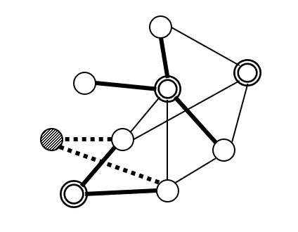
(a) The first level of Baswana-Sen in the original graph.

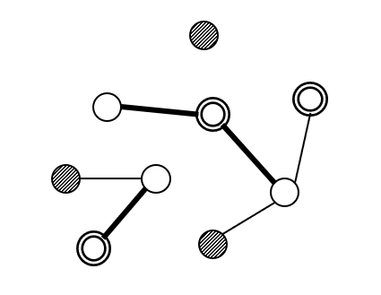
(b) The first level of our modified Baswana-Sen, as executed by the large machine on the sub-sampled graph. The large machine is able to re-cluster fewer nodes than true Baswana-Sen (Fig. 1(a) above), and as a result, it adds fewer edges and removes more nodes.

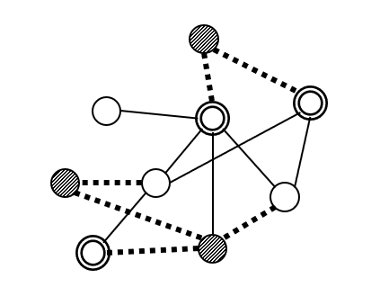
(c) The first level of our modified Baswana-Sen, as executed on the small machines after learning the cluster to which each node is assigned by the large machine, and which nodes were removed. Since the large machine removes more nodes than true Baswana-Sen, the small machines add more edges than true Baswana-Sen.

Figure 1: The first level of Baswana-Sen, the original version and our modified version. Initially, each node forms its own cluster ($C_{0}=V$). Nodes selected for $C_{1}$ are indicated with double circles. Nodes that are no longer clustered ($C_{0}\setminus C_{1}$) must either be re-clustered by adding them to some neighboring cluster (these nodes are shown as white circles), or removed (these nodes are shown as a striped circle). Bold lines indicate edges added to the spanner when a node is re-clustered, and dashed lines indicate edges added to the spanner when a node is removed.

Implementing modified Baswana-Sen in the Heterogeneous MPC model

Assume that the input to the modified Baswana-Sen algorithm is a graph $G=(V,E)$ stored on the small machines, an integer $1\leq k\leq\log{n}$, and a sampling probability $p\in(0,1)$ such that $p\cdot|E|=\tilde{O}(n)$. To implement modified Baswana-Sen, we have the small machines sample the subgraphs $G_{1},\ldots,G_{k}$ locally (sampling each edge indenendently with probability $p$), and send them to the large machine. This suffices for the large machine to carry out lines 2–2 of Algorithm 2, where we compute the clusters, as this part of the algorithm depends only on $G_{1},\ldots,G_{k}$ and does not require knowledge of the full graph $G$.

After executing lines 2–2, the large machine sends to the small machines the clusters that it computed during the run, specifying for each node $v$ and level $i$ the center $c_{i}(v)$ of the cluster to which $v$ belonged in level $i$: each small machine that stores some edge adjacent to $v$ receives the centers $(c_{0}(v),\ldots,c_{k}(v))$. This is done in constant number of rounds using Claim 3.

Finally, the small machines carry out lines 2–2 of Algorithm 2: we add, for each vertex $v$ that was removed in some step $i$, one edge connecting $v$ to each level-$(i-1)$-cluster that $v$ is adjacent to. To find these edges, each small machine $M$ creates a set of candidates,

$$A_{M} =\left\{(v,c,u)\in V^{3}:\exists i\ c_{i-1}(v)\neq\bot,c_{i}(v)=\bot,\right.$$

$$\qquad\left.c_{i-1}(u)=c\neq\bot,\text{ and }\left\{u,v\right\}\in E\right\}$$

The candidate $(v,c,u)$ represents the fact node $v$ was removed at level $i$, and at that point it was adjacent to a vertex $u$ belonging to a level-$(i-1)$ cluster centered at $c$. The edge $\left\{u,v\right\}$ is thus a candidate for being added to the spanner, but we must ensure that we take only one edge per level-$(i-1)$ cluster that $v$ is adjacent to: using Claim 2, in $O(1)$ rounds we select for each vertex $v$ and center $c$ the smallest vertex $u$ such that $(v,c,u)$ is a candidate, and add edge $\left\{u,v\right\}$ to the spanner.

Putting everything together

The variant of Baswana-Sen that we introduced above is particularly suitable for computing spanners over the clustering graphs in the Heterogeneous MPC model. Recall that each of the clustering graphs $A_{i}$ contains at most $O(n\cdot i/2^{i})$ vertices and $O(n2^{i})$ edges, except for $A_{0}$, which has $O(n)$ vertices and $O(n)$ edges. Accordingly, we set our sampling probability to $p_{i}=\min\left\{k^{2}i^{1+1/k}/2^{i},1\right\}$. Now there are three cases:

• For $i=0$, we can afford to send the entire edge set $E_{0}$ to the large machine, since $|E_{0}|=O(n)$.

• For $i>0$ such that $p_{i}=1$, we can also afford to send the entire edge set $E_{i}$ to the large machine: if $p_{i}=1$, then $2^{i}\leq k^{2}i^{1+1/k}\leq k^{2}i^{2}$, and thus $|E_{i}|=O(n2^{i})=O(k^{2}i^{2}n)$. Since $k=O(\log{n})$ and $i\leq\log\Delta$, this means that $|E_{i}|=O(n\operatorname{\mathrm{polylog}}{n})$. Thus, the large machine can compute an optimal spanner of size $O((ni/2^{i})^{1+1/k})$.

• For $i>0$ such that $p_{i}=k^{2}i^{1+1/k}/2^{i}<1$, we use modified Baswana-Sen. In this case we have $p_{i}\cdot|E_{i}|=O(k^{2}i^{1+1/k}/2^{i}\cdot n2^{i})=O(k^{2}i^{1+1/k}n)=\tilde{O}(n)$, so indeed after sub-sampling the graph with probability $p_{i}$, the resulting edge set can fit on the large machine. By Lemma 4.3, we obtain a $(2k-1)$-spanner $H_{i}$ of expected size $O(k(ni/2^{i})^{1+1/k}\cdot 2^{i}/k^{2}i^{1+1/k})=O(n^{1+1/k}/k2^{i/k})$.

Taking the maximum of the options above, for each $i\geq 1$, the spanner $H_{i}$ constructed for the $i$-th clustering graph has expected size

$$h_{i}=O\left(n^{1+1/k}\left(\left(\frac{i}{2^{i}}\right)^{1+1/k}+\frac{1}{k2^{i/k}}\right)\right).$$

Using the fact that $\sum_{i=0}^{\infty}(i^{2}/2^{i})=6$ and $\sum_{i=0}^{\infty}1/(k2^{i/k})<1/(1-1/2^{1/k})<1$, we have that $\sum_{i=0}^{\infty}h_{i}=O(n^{1+1/k})$ in expectation.

Thus, the $(6k-1)$-spanner $H$ of $G$ obtained by combining the spanners of the individual clustering graphs has an expected size of $O(n^{1+1/k})$.

5 Maximal Matching in $O(\sqrt{\log(m/n)}\log\log(m/n))$ Rounds

In this section we give an algorithm for maximal matching in the Heterogeneous MPC model, and show:

Theorem 5.1.

There is an $O(\sqrt{\log{d}}\log\log{d})$-round algorithm in the Heterogeneous MPC model that computes a maximal matching with high probability in graphs of average degree $d$.

In our algorithm, we rely on the following claim from [33]:

Lemma 5.2 (Section 3.6 and Proof of Theorem 3.2 in [33]).

In sublinear MPC, it is possible in $O(\sqrt{\log\Delta}\log\log{\Delta})$ rounds to find a matching $M$, such that the number of edges with both endpoints unmatched in $M$ is at most $m/\Delta^{10}\leq n$.

After finding the matching guaranteed by Lemma 5.2, the number of edges that have both endpoints unmatched is small enough to store all of them on the large machine and compute a maximal matching over them. Thus we obtain the following immediate corollary in Heterogeneous MPC:

Corollary 5.3.

In Heterogeneous MPC, it is possible to find a maximal matching in $O(\sqrt{\log\Delta}\log\log{\Delta})$ rounds.

This is not yet our final result, since we want an algorithm whose running time depends on the average degree $d$ rather than the maximum degree $\Delta$. Thus, we proceed in three phases:

Phase 1:

We divide the vertices into low-degree vertices, $V_{\ell}=\left\{\ v:\deg(v)\leq d^{2}\right\}$, and high-degree vertices, $V_{h}=V\setminus V_{\ell}$. There are at most $n/d$ high-degree vertices: by Markov, if we choose a random vertex $v$, we have $\Pr[\deg(v)\geq d^{2}]\leq 1/d$, and therefore $|V_{h}|\leq n/d$.

Using only the small machines, we apply the procedure of Corollary 5.3 to the graph induced by the low-degree vertices $V_{\ell}$, to obtain a maximal matching $M_{1}$. As the maximum degree in this graph is $d^{2}$, this takes $O(\sqrt{\log{d}}\log\log{d})$ rounds. The small machines send $M_{1}$ to the large machine.

Phase 2:

For each vertex $v\in V_{h}$, the large machine collects $2d\log{n}$ random incident edges of $v$ (including both neighbors in $V_{\ell}$ and in $V_{h}$), or all edges incident to a $v$ if $\deg(v)<2d\log{n}$. Denote this set by $E^{\prime}(v)$. To do this, each small machine assigns a uniformly random rank $r(e)\in_{U}\{1,\dots,n^{5}\}$ to each edge $e$ that it stores. With probability $1-1/n$ each edge is assigned a unique rank, and we then select the $2d\log{n}$ lowest-ranked edges incident to each vertex (or all edges incident to the vertex) and send those edges to the large machine. This is done in a manner similar to Section 3 (in the MST algorithm, where the large machine collects a fixed number of the lightest outgoing edges of each vertex). Note that since $|V_{h}|\leq n/d$, the total number of edges collected by the large machine is $O(n/d\cdot d\log{n})=O(n\log{n})$.

The large machine greedily constructs a matching $M_{2}$, as follows: initially, $M_{2}=\emptyset$. The large machine orders the vertices $V_{h}$ arbitrarily, and goes over the vertices in this order. For each vertex $u$ examined, if $u$ is still unmatched in $M_{1}\cup M_{2}$ and there is an edge $\left\{u,v\right\}\in E^{\prime}(u)$ such that $v$ is also unmatched in $M_{1}\cup M_{2}$, then the large machine chooses one such neighbor $v$, and adds $\left\{u,v\right\}$ to $M_{2}$.

After constructing $M_{2}$, the large machine informs the small machines about vertices that are matched in $M_{1}\cup M_{2}$: for each vertex $v$ and small machine $M$ that stores some edge adjacent to $v$, the large machine informs $M$ whether or not $v$ is matched in $M_{1}\cup M_{2}$. This is done using Claim 3.

Phase 3:

Let $E^{\prime\prime}$ be the set of edges that have both endpoints unmatched in $M_{1}\cup M_{2}$. Each small machine sends the large machine a count of the number of edges in $E^{\prime\prime}$ that it stores, and the large machine sums these counts to compute $|E^{\prime\prime}|$. If $|E^{\prime\prime}|>2n$, the algorithm fails. Otherwise, the small machines send $E^{\prime\prime}$ to the large machine, and the large machine computes a maximal matching $M_{3}$ over $E^{\prime\prime}$.

The final output of the algorithm is $M_{1}\cup M_{2}\cup M_{3}$. This is indeed a maximal matching of $G$, as in Phase 3 the large machine receives all edges whose two endpoints remain unmatched in $M_{1}\cup M_{2}$, and $M_{3}$ completes $M_{1}\cup M_{2}$ into a maximal matching.

To prove that the algorithm succeeds w.h.p., we need only to show that it does not fail in Phase 3, i.e., that the number of edges the small machines need to send to the large machine is not too large:

Lemma 5.4.

After Phase 2, w.h.p. the total number of edges whose two endpoints are unmatched in $M_{1}\cup M_{2}$ is at most $2n$.

Proof..

First, since $M_{1}$ is a maximal matching over the subgraph induced by $V_{\ell}$, no edge that has both endpoints in $V_{\ell}$ still has both endpoints unmatched in $M_{1}\cup M_{2}$. Thus, we consider only edges that have at least one endpoint in $V_{h}$. Let $u_{1},\ldots,u_{k}$ be the vertices of $V_{h}$, in the order they are processed by the large machine when constructing $M_{2}$, and let $R_{i}$ be the randomness used to select the $\Theta(d\log{n})$ random neighbors of $u_{i}$ sent to the large machine.

If $\deg(u_{i})<2d\log{n}$, then no incident edges of $u_{i}$ have both endpoints unmatched after $u_{i}$ is processed: in this case the large machine is sent all incident edges of $u_{i}$, and when it processes $u_{i}$, if there is some edge $\left\{u_{i},v\right\}\in E$ such that $u_{i},v$ are both unmatched, the large machine adds some incident edge of $u_{i}$ to the matching. Following this step, all incident edges of $u_{i}$ have at least one endpoint matched.

Suppose $\deg(u_{i})\geq 2d\log{n}$, and let $B_{i}$ be the event that at the point where $u_{i}$ is processed by the large machine, $u_{i}$ and at least a $1/d$-fraction of $u_{i}$’s neighbors are still unmatched, but the large machine is not able to find an edge $\left\{u_{i},v\right\}\in E^{\prime}(u_{i})$ such that $v$ is unmatched. If $B_{i}$ does not occur, then either at most $\deg(u_{i})/d$ incident edges of $u_{i}$ have both endpoints unmatched after $u_{i}$ is processed, or the large machine has found an edge $\left\{u_{i},v\right\}\in E^{\prime}(u_{i})$ such that $v$ is unmatched.

Fix the randomness $R_{1},\ldots,R_{i-1}$ of the nodes preceding $u_{i}$, and assume that given this fixing, node $u_{i}$ is unmatched after processing and has at least $\deg(u_{i})/d$ unmatched neighbors when it is processed (otherwise, the event $B_{i}$ does not occur). The randomness used to select $E^{\prime}(u_{i})$ is independent of $R_{1},\ldots,R_{i-1}$. Each time we select the next random neighbor of $u_{i}$ for $E^{\prime}(u_{i})$, as long as we have not yet selected an unmatched neighbor, the probability that we select an unmatched neighbor is at least $(\deg(u_{i})/d)/\deg(u_{i})=1/d$. Thus, the probability that we fail to select any of $u_{i}$’s unmatched neighbors is at most $(1-1/d)^{2d\log{n}}\leq e^{-2\log{n}}<1/n^{2}$. Since this holds for every fixing of $R_{1},\ldots,R_{i-1}$, we have $\Pr[B_{i}]\leq 1/n^{2}$, and by union bound, the probability that none of the events $B_{i}$ for nodes $u_{i}$ with $\deg(u_{i})\geq 2d\log{n}$ occur is at least $1-1/n$. In this case, the total number of edges that still have both endpoints unmatched after the large machine finishes processing the nodes of $V_{h}$ is at most $\sum_{i=1}^{k}\deg(u_{i})/d\leq 2nd/d=2n$. ∎

This concludes our algorithm. For the more general setting where the large machine has memory of size $\tilde{O}(n^{1+f(n)})$, the MapReduce algorithm of [44] can be adapted to find a maximal matching as well:

Theorem 5.5.

Given a single machine with memory $\tilde{\Omega}(n^{1+f(n)})$, and $\Omega(m/n^{\gamma})$ machines with memory $\tilde{\Omega}(n^{\gamma})$, there is an $O(1/f(n))$-round algorithm in the Heterogeneous MPC model that computes a maximal matching with high probability.

Proof of theorem 5.5..

We follow the algorithm of [44] for finding a maximal matching the MapReduce model. By [44] Lemma 3.1, if we sample each edge of an input graph $G$ independently with some probability $p$ and find a maximal matching $M$ over the sampled subgraph $G_{p}$, the number of edges in $G$ whose both end-points are unmatched in $M$ (i.e., potentially can be added to the matching) is $O(n/p)$ with high probability.

The algorithm is recursive. If the current graph has $O(n^{1+f(n)})$ edges, we reach the stop condition, and send all edges to the large machine to find a maximal matching. Otherwise, we sample each edge independently with probability $p=\frac{1}{n^{f(n)}}$ to create a random subgraph $G_{p}$. When the algorithm returns, a maximal matching $M$ of the graph $G_{p}$ is known to the large machine. The large machine notifies the small machines about the matched vertices in $M$ as described in Claim 3. Denote the set of edges that can potentially be added to the matching $M$ by $E_{M}$. From the statement in the beginning of the proof, we have that $|E_{M}|=O(n^{1+f(n)})$, thus they can fit the memory of the large machine. Finally, the large machine computes the matching $M_{2}$ such that $M\subseteq M_{2}$ and returns $M_{2}$ from the recursive call. The algorithm takes at most $O(1/f(n))$ recursive iterations, at which point it reaches the stop condition.

∎

6 Conclusion and Future Directions

In this first work we focused on a heterogeneous MPC regime where we add a single machine with near-linear (or larger) memory to the sublinear regime. We showed that even a single machine can make a big difference in the round complexity of fundamental graph problems, circumventing several conditional hardness results. This is only one special case of the heterogeneous setting, and in general one can ask — just how many machines of each memory size (sublinear, near-linear or superlinear) are required to efficiently solve a given problem? And if we allow the total memory use of all the machines to exceed the input size (as in, e.g., [15, 41, 29]), does that help even further? To study these questions, we propose a more general version of the heterogeneous model, parameterized by the total memory of each type of machine: the $(S_{\text{sub}}(m,n),S_{\text{lin}}(m,n),S_{\text{sup}}(m,n))$-Heterogeneous MPC model has machines with sublinear, near-linear or super-linear memory, using a total of $\tilde{\Theta}(S_{\text{sub}}(m,n)),\tilde{\Theta}(S_{\text{lin}}(m,n))$ and $\tilde{\Theta}(S_{\text{sup}}(m,n))$ memory, respectively. (This means that the number of near-linear machines is $\tilde{\Theta}(S_{\text{lin}}(m,n)/n)$, while the number of sublinear and near-linear machines is $\tilde{\Theta}(S_{\text{sub}}(m,n)/n^{\gamma})$ and $\tilde{\Theta}(S_{\text{sup}}(m,n)/n^{1+\gamma})$, respectively, for some parameter $\gamma\in(0,1)$.) From this more general perspective, the model that we studied in this paper is the $(\tilde{\Theta}(m),\tilde{\Theta}(n),0)$-Heterogeneous MPC model.

We mention several concrete open problems. First, it is interesting to ask whether MST and maximal matching can be solved in the Heterogeneous MPC model (the specific version that we studied in this paper) in the same round complexity as in the near-linear model, and whether this holds for the other problems that we did not address here — e.g., those whose conditional hardness is proven in [29]. Another question is whether problems that appear to require polynomial time in the near-linear model, but can be efficiently solved in the superlinear model, can also be efficiently solved in a hybrid near-linear / superlinear model where we have many near-linear machines and a small number of superlinear machines. Finally, it is very interesting to ask whether any conditional hardness results can be strengthened to yield non-trivial lower bounds for the heterogeneous model, in order to better characterize the benefit resulting from adding one near-linear machine to the sublinear MPC model.

Appendix A Constructing the Clustering Graphs from Section 4

We provide a more detailed description of the clustering graphs from [22].

A star in a graph $G$ is a tree-shaped subgraph of $G$ with one or more vertices and diameter at most $2$.

For graph $G=(V,E)$ of maximum degree $\Delta$, let $S_{0},...,S_{\log\Delta-1}$ be sets of stars in $G$. From the star definition, each $s\in S_{i}$ is either a single vertex $u\in V$, or a center vertex $u\in V$ surrounded by a set of vertices connected to it. In both cases, we call $u$ the center of the star $s$, and denote it by $c(s)=u$. Moreover, for $v\in V$ denote by $s_{i}(v)$ the center of star to which $v$ belongs in the set $S_{i}$, i.e., if $v$ belongs to the star $s\in S_{i}$ then $s_{i}(v)=c(s)$ (in case $v$ does not belong to any of the stars in $S_{i}$, $s_{i}(v)$ is undefined).

Now, define the corresponding clustering graphs $A_{0},...,A_{\log\Delta-1}$ of the sets $S_{0},...,S_{\log\Delta-1}$ in the following way: $V_{i}=\left\{c(s)\mid s\in S_{i}\right\}$, and

$$E_{i} =\{(c,c^{\prime})\mid\exists(u,v)\in E:s_{i}(u)=c,s_{i}(v)=c^{\prime},$$

$$\min\left\{\deg(u),\deg(v)\right\}\in[2^{i},2^{i+1})\}$$

Given an edge $(c,c^{\prime})\in E_{i}$, let $E_{G}((c,c^{\prime}))\in E$ be the lexicographically-smallest edge $(u,v)\in E$ such that $s_{i}(u)=c$, $s_{i}(v)=c^{\prime}$ and $\min\left\{\deg(u),\deg(v)\right\}\in[2^{i},2^{i+1})$. (such an edge must exist, from the definition of $E_{i}$.) Similarly, for a set of edges $X\subseteq E_{i}$, we let $E_{G}(X)=\bigcup_{(c,c^{\prime})\in X}E_{G}((c,c^{\prime}))$.

Lemma A.1 ([22] Section 4).

For a graph $G=(V,E)$ of maximum degree $\Delta$, there exist star sets $S_{0},...,S_{\log\Delta-1}$ and corresponding clustering graphs $A_{i}=(V_{i},E_{i})$ such that:

• $|V_{0}|=n,|E_{0}|=O(n)$, and for each $0\leq i\leq\log\Delta-1$, $|V_{i}|=O(ni/2^{i})$ and $|E_{i}|=O(n\cdot 2^{i})$.

• For any $e\in E$, there exists $0\leq i\leq\log\Delta-1$ such that $e$ is either contained in some star $s\in S_{i}$, or $e\in E_{i}$.

• If a vertex $v\in V$ belongs to two stars $s\in S_{i}$ and $s^{\prime}\in S_{j}$ for $i\neq j$ such that $v\not=c(s)$ and $v\not=c(s^{\prime})$, then $c(s)=c(s^{\prime})$.

Let $A_{0},...,A_{\log\Delta-1}$ be the clustering graphs from Lemma A.1. The following lemma states that by combining individual spanners for these clustering graphs we can obtain a spanner for the original graph:

Lemma A.2 ([22] Section 4.4).

Let $H_{0},\dots,H_{\log\Delta-1}$ be $(2k-1)$-spanners of $A_{0},\dots,A_{\log\Delta-1}$, respectively. Let $E_{stars}^{i}=\cup_{s\in S_{i}}\left\{e\mid e\in s\right\}$ for all $0\leq i\leq\log\Delta-1$. Then, $H=\bigcup_{0\leq i\leq\log\Delta-1}E_{G}(H_{i})\cup E_{stars}^{i}$ is a $(6k-1)$-spanner of $G$, of size at most $O(n)+\sum_{i=0}^{\log\Delta-1}|H_{i}|$.

Clustering graphs in the Heterogeneous MPC.

Algorithm 3 constructs the clustering graphs $A_{0},...,A_{\log\Delta-1}$ from Lemma A.1 in $O(1)$ rounds in the Heterogeneous MPC model in the same manner as [22]. We define the sets $U_{i}=\{v\in V\mid 2^{i}\leq deg(v)\leq 2^{i+1}\}$ for $0\leq i\leq\log\Delta$. The set $B_{i}\subseteq V$ is called a hitting-set of $U_{i}$ if for each $v\in U_{i}$, either $v\in B_{i}$ or $v$ has a neighbor $u\in B_{i}$. Algorithm 3 starts by computing the hitting-set $B_{i}$ for each $U_{i}$. Then, the clustering graphs $A_{i}=(V_{i},E_{i})$ for each $0\leq i\leq\log\Delta-1$ are constructed based on these hitting-sets. We note that for each $e=(c,c^{\prime})\in E_{i}$, we attach the lexicographically-smallest edge $(u,v)\in E$ that cause $e$ to be contained in $E_{i}$, so that in the end, for each $(c,c^{\prime})\in H_{i}$ we will be able to compute $E_{G}((c,c^{\prime}))$ and add it to the final spanner $H$ of $G$.

Appendix B Pseudocode

In this section, we provide pseudo-code for key procedures of Section 3 in the Heterogeneous MPC model, namely, the doubly-exponential Borůvka procedure, and a procedure for identifying the $F$-light edges.

We also provide the pseudo-code for Section 4, for constructing the clustering graphs and for constructing the spanner.

[htbp]    DoublyExpBoruvka($G=(V,E,w),k$) Input :  $G$ is a weighted undirected graph, k is an integer Output : $G_{k}$ is the contracted graph resulting from applying $k$ iterations of Borůvka, $F$ are the edges that were used for contraction  $F\leftarrow\phi,V_{0}\leftarrow V,E_{0}\leftarrow E,\forall v\in V:c_{0}(v)=v$

1  // $c_{i}:V\rightarrow V_{i}$ map each vertex $v\in V$ to the vertex into which it was merged in $V_{i}$ for $0\leq i\leq k-1$ do

2      small machines do in parallel:

           sort all edges $E_{i}$ primarily by $1^{st}$ endpoint id, then by weight, then by the $2^{nd}$ endpoint id

3            // Claim 1

4           large machine:

5                locally compute:

6                     foreach $v\in V$ do

                         compute $deg_{out}(v)$ and $M_{first}(v)$

7                           // Claim 4 foreach small machine $M$ do

8                              compute $k(v,M)\leftarrow$ out of $v$’s lightest $\min(2^{2^{i}},\deg_{\mathrm{out}}(v))$ edges, the number of edges that are stored on $M$

9                              

10                              

11                               disseminate $k(v,M)$ to small machine $M$ that holds an adjacent edge of $v$ for each $v\in V$

12                               small machines do in parallel:

13                                    foreach $v\in V$ and machine $M$ do

14                                        $E_{lightest}\leftarrow$the $k(v,M)$ lightest edges of $v$ that are stored on $M$

15                                         send $E_{lightest}$ to the large machine

16                                        

17                                         large machine:

18                                              locally compute:

19                                                   $F_{contracted}\leftarrow\phi$, $V_{i+1}\leftarrow\phi$

20                                                   foreach $e\in E_{lightest}$ from the lightest to the heaviest do

21                                                        if $e=(u,v)$ dose not create a cycle in $F_{contracted}$ then

22                                                             $F_{contracted}\leftarrow F_{contracted}\cup\{(u,v)\}$

23                                                             $V_{i+1}\leftarrow V_{i+1}\cup\left\{\min\left\{u,v\right\}\right\}$

                                                             $c_{i}^{{}^{\prime}}(u),c_{i}^{{}^{\prime}}(v)\leftarrow\min\{u,v\}$

24                                                              // $c^{\prime}_{i}:V_{i}\rightarrow V_{i+1}$ map each $v\in V_{i}$ to the vertex into which it was merged in $V_{i+1}$ $F\leftarrow F\ \cup\{(u^{\prime},v^{\prime})\in E\mid c_{i}(u^{\prime})=u,c_{i}(v^{\prime})=v,(u^{\prime},v^{\prime})$ is the minimum weight such edge}

25                                                            

26                                                            

27                                                            

                                                             disseminate $c_{i}^{{}^{\prime}}(v)$ to each machine that holds an adjacent edge of $v$ for each $v\in V$

28                                                              // Claim 3

29                                                             small machines do in parallel:

                                                                  aggregate $E_{i+1}\leftarrow\{(u^{\prime\prime},v^{\prime\prime},w(u,v))\mid(u,v)\in E_{i},c_{i}^{{}^{\prime}}(u)=u^{\prime\prime},c_{i}^{{}^{\prime}}(v)=v^{\prime\prime}$, $u^{\prime\prime}\not=v^{\prime\prime}$ and $(u,v)$ is the minimum weight edge for which the previous conditions hold}

30                                                                   // Claim 2 foreach $v\in V$ do

31                                                                       $c_{i+1}(v)=c_{i}^{\prime}(c_{i}(v))$

32                                                                      

33                                                                      

34                                                                      

35                                                                       output $(G_{k}=(V_{k},E_{k},w),F)$

 

[htbp]    F-LightEdges($G=(V,E,w),F$) Input : $G$ is a weighted, undirected graph, $F$ is a spanning forest of $G$ stored on the large machine Output : $E_{light}$ are the $F$-light edges in $G$

1  // see section 3 for $F$-light, $\mathcal{M}_{\mathrm{flow}}$ and $\mathcal{D}_{\mathrm{flow}}$ definitions  $E_{light}\leftarrow\phi$

2 large machine:

3      locally compute:

4           compute labels $L:V\rightarrow\left\{0,1\right\}^{O(\log^{2}n)}$ by applying $\mathcal{M}_{\mathrm{flow}}(F)$

5          

           disseminate $L(v)$ to each small machine $M$ that holds an edge incident to $v$ for each $v\in V$

6            // Claim 3

7           small machines do in parallel:

8                foreach $(u,v)\in E$ do

9                     if $w(u,v)\leq\mathcal{D}_{\mathrm{flow}}(L(u),L(v))$ then

10                          $E_{light}\leftarrow E_{light}\cup\left\{(u,v)\right\}$

11                         

12                         

output $E_{light}$  

1

Input : $G$ is a weighted, undirected graph

Output : $H$ are the edges used to construct the clustering graphs, $A_{0},...,A_{\log\Delta-1}$ are the clustering graphs

2  

3large machine:

4      locally compute:

5           for $1\leq j\leq\log(n)$ do

6                $D_{0}^{j}\leftarrow V$

7                for $1\leq i\leq\log\Delta-1$ do

8                     $D_{i}^{j}\leftarrow$ sample each $u\in V$ w.p. $p=\frac{i}{2^{i}}$

9                    

10                    

11                    

12                    

                    disseminate $D_{i}^{j}$ to each machine that holds an incident edge of $v\in D_{i}^{j}$ for each $v\in V$, $1\leq j\leq\log(n)$ and $1\leq i\leq\log\Delta-1$

                      // Claim 3

13                    

14                    

15                    small machines do in parallel:

16                          for $1\leq j\leq\log(n)$ do in parallel

17                               for $1\leq i\leq\log\Delta-1$ do in parallel

                                    aggregate $D_{i}^{j}\leftarrow D_{i}^{j}\cup\{u\in V\mid 2^{k}\leq deg(u)\leq 2^{k+1},i\leq k,\ u$ has no neighbor in $D_{i}^{j}\}$

                                     // Claim 2

18                                    send $D_{i}^{j}$ to the large machine

19                                   

20                                   

21                                   

22                                   

23                                   large machine:

24                                         locally compute:

25                                              for $1\leq i\leq\log\Delta-1$ do

26                                                   $D_{i}\leftarrow D_{i}^{j}$ such that $D_{i}^{j}=\operatorname*{arg\,min}_{1\leq j\leq\log{n}}\{|D_{i}^{j}|\}$

27                                                  

28                                                  

29                                                  

                                                  disseminate $D_{i}$ to each machine that holds an incident edge of $v\in D_{i}$ for each $v\in V$ and $1\leq i\leq\log\Delta-1$

                                                    // Claim 3

30                                                  

31                                                  

32                                                  small machines do in parallel:

33                                                        for $0\leq i\leq\log\Delta-1$ do in parallel

34                                                             $B_{i}\leftarrow\cup_{j=i}^{\log\Delta-1}D_{j}$

35                                                            

36                                                             foreach $u\in V$ do

                                                                  aggregate $i_{u}\leftarrow\max\{i\mid u\in B_{i}$ or $N(u)\cap B_{i}\not=\emptyset\}$

                                                                   // Claim 2

37                                                                  if $u\in B_{i_{u}}$ then

38                                                                       $\sigma_{u}\leftarrow u$

39                                                                       for $0\leq i\leq i_{u}$ do in parallel

40                                                                            $V_{i}\leftarrow V_{i}\cup\{u\}$

41                                                                           

42                                                                           

43                                                                            else

44                                                                                 $\sigma_{u}\leftarrow$ a random neighbor of $u$ in $B_{i_{u}}$

45                                                                                 $H\leftarrow(u,\sigma_{u})$

46                                                                                

47                                                                                

48                                                                                 foreach $(u,v)\in E$ do

49                                                                                      if $\min\{\deg(u),\deg(v)\}=2^{i}$ and $\sigma_{u}\not=\sigma_{v}$ then

50                                                                                           $E_{i}\leftarrow(\sigma_{u},\sigma_{v})$

51                                                                                          

52                                                                                          

53                                                                                          

54                                                                                          

55                                                                                          output $H$ and $(V_{i},E_{i})$ for $0\leq i\leq\log\Delta-1$

56                                                                                          

Algorithm 3 ClusteringGraphs(G)

1

Input : $G$ is a weighted, undirected graph, $k$ is an integer

Output : $H$ is an $O(k)$-spanner of $G$ of expected size $O(n^{1+\frac{1}{k}})$

2  

$H,A_{0},...,A_{\log\Delta-1}\leftarrow$ ClusteringGraphs($G$)

  // $A_{i}=(V_{i},E_{i})$

3

4for $0\leq i\leq\log\Delta-1$ do in parallel

5      if  $i=0$ or $p_{i}=\frac{k^{2}i^{1+1/k}}{2^{i}}>1$ then

6           small machines do in parallel:

7                send $A_{i}$ to the large machine

8               

9               

10               large machine:

11                     locally compute:

12                          $H_{i}\leftarrow(2k-1)$-spanner of $A_{i}$

13                          $H\leftarrow H\cup E_{G}(H_{i})$

                         

                           // $E_{G}(H_{i})=\{(u,v)\in E\ \mid\min\{\deg(u),\deg(v)\}=2^{i},\ (\sigma_{u},\sigma_{v})\in H_{i}$ and $(u,v)$ is the minimum weight such edge$\}$

14                         

15                         

16                         

17                          else

18                               small machines do in parallel:

19                                    for $1\leq j\leq k-1$ do in parallel

20                                         $E_{i}^{j}\leftarrow$ sample each $e\in E_{i}$ w.p. $p_{i}=\frac{k^{2}i^{1+1/k}}{2^{i}}>1$

21                                         send $A_{i}^{j}=(V_{i},E_{i}^{j})$ to the large machine

22                                        

23                                        

24                                        

25                                        large machine:

26                                              locally compute:

27                                                   $H_{i}\leftarrow$ compute lines 2–2 of ModifiedBaswanaSen($A_{i},k,1/2^{i}$) using the sampled subgraphs $(A_{i}^{1},...,A_{i}^{k-1})$

28                                                   foreach $v\in V_{i}$ do

29                                                        $l_{i}^{v}\leftarrow(i,c_{0}(v),...,c_{t-1}(v))$ such that $v$ stopped being clustered at iteration $t$, $c_{j}(v)$ is $v$’s cluster center at iteration $j$

30                                                       

31                                                       

32                                                       

                                                       disseminate $l_{i}^{v}$ to each machine that holds edges of $v$ for each $v\in V$

                                                         // Claim 3

33                                                       

34                                                       

35                                                       small machines do in parallel:

36                                                             foreach $(u,v)\in E_{i}$ do

37                                                                  if $|l_{i}^{v}|>|l_{i}^{u}|$ then

38                                                                       Create a record $(i,u,c_{t-1}(v),v)$

39                                                                      

                                                                      

                                                                        // $u$ stopped being clustered before $v$ at iteration $t$

40                                                                       else if $|l_{i}^{u}|>|l_{i}^{v}|$ then

41                                                                            Create a record $(i,v,c_{t-1}(u),u)$

42                                                                           

                                                                           

                                                                             // $v$ stopped being clustered before $u$ at iteration $t$

43                                                                           

44                                                                            foreach $u\in V_{i}$ and a cluster $c$ do

                                                                                 aggregate $v\leftarrow\operatorname*{arg\,min}_{v\in V_{i}}\{(i,u,c_{t-1}(v),v)\mid c_{t-1}(v)=c\}$

                                                                                  // Claim 2

45                                                                                 $H_{i}\leftarrow H_{i}\cup\left\{(u,v)\right\}$

46                                                                                

47                                                                                 $H\leftarrow E_{G}(H_{i})$

48                                                                                

49                                                                                

50                                                                                

output $H$

Algorithm 4 Spanner($G,k$)

Appendix C Prior Works That Extend to the Heterogeneous MPC Model

Several prior works in the near-linear MPC model, while not explicitly presented for a model like Heterogeneous MPC, easily translate to this model. In this section, we give an overview of these results, and provide some relevant adaptation details.

C.1 Connectivity in $O(1)$ Rounds

In this subsection we show how by leveraging the existing techniques of linear sketches and $l_{0}$-sampling which are mostly used in the context of streaming algorithms [36, 1, 2, 38, 39, 46], as well as in the congested clique ([35], we get constant-round algorithms for connectivity in the Heterogeneous MPC model. The implementation is very similar to the implementation in near-linear MPC, except that now the edges associated with a single vertex may be stored across more than a single machine; using linear sketches, this is trivial to overcome.

Theorem C.1.

There is an $O(1)$-round algorithm to identify the connected components of a graph with high probability in the Heterogeneous MPC.

Proof..

We apply the connectivity algorithm from  [1] which is based on linear-sketches for $\ell_{0}$-sampling, as stated originally in [36], but replacing the shared randomness assumed in [36] with $O(\log n)$-wise independence [1], so that one machine can generate $O(\operatorname{\mathrm{polylog}}n)$ random bits, disseminate them to all the other machines, and these are then used to generate all the sketches. The sublinear machines compute a linear sketch $s(v)$ for each node $v\in V$. This sketch can be used to sample a random neighbor of $v$, and for a set of nodes $S=\{v_{1},...,v_{k}\}$, the sketch $s=s(v_{1})+...+s(v_{k})$ can be used to randomly sample an edge from $E[S,V\backslash S]$. The total number of bits required for all nodes sketches is $O(n\log^{3}(n))$, thus, all sketches can be stored in the near-linear-spaced machine which can then simulate the connectivity algorithm of [1]. During the algorithm, nodes from the same connected component are merged using the sampled edges into contracted virtual nodes. The nodes in the final contracted graph represent the connected components of the input graph.

In order to construct a sketch for some node $v$, it is required to know all neighbors of $v$. But, we cannot assume that the sublinear machine has a sufficient memory to hold all of $v$’s neighbors. Instead, we use the following property of the linear sketches:

Property 1.

Let $G_{1},\dots,G_{k}\subseteq G$ such that $N(v)=N_{G_{1}}(v)\uplus\dots\uplus N_{G_{k}}(v)$, and let $s_{1}(v),\dots,s_{k}(v)$ be linear sketches in these graphs, then $s(v)=\sum_{i=1}^{k}s_{i}(v)$ is a linear sketch of $v$.

Each sublinear machine computes a partial-sketch for each $v\in V$ based on the neighbors of $v$ which it holds. Using Claim 2, the final sketches are constructed by adding up all the partial sketches, which takes constant number of rounds. ∎

C.1.1 $(1+\epsilon)$-Approximation of MST in $O(1)$ Rounds

Theorem C.2.

For any constant $\epsilon>0$, there is an $O(1)$-round algorithm to compute an $(1+\epsilon)$-approximation of the minimum spanning tree in the Heterogeneous MPC.

Proof..

We follow the known reduction from [1] to reduce the problem of estimating the weight of the minimum spanning tree to the problem of counting the number of connected components in the graph. This approach requires applying the connectivity algorithm in parallel over $O(\log(n))$ subgraphs. This takes constant number of rounds using the connectivity algorithm from theorem C.1. ∎

C.2 Exact Unweighted Minimum Cut in $O(1)$ Rounds

In this subsection, we give an overview of the result of [32] for computing the minimum cut of an unweighted graph.

Theorem C.3.

There is an $O(1)$-round algorithm in the Heterogeneous MPC model that with high probability computes the minimum cut of an unweighted graph.

Proof..

The heart of the algorithm is a contraction process, which consists of two parts:

1. $2$-out contraction: Each node $v\in V$ samples two edges. Then, we contract all connected components of the graph induced over the sampled edges, while allowing parallel edges.

2. Random-sampling contraction: For a multi-graph of minimum degree $\delta$, we contract a set of edges $E_{p}$, to which we include each $e\in E$ independently with probability $p=\frac{1}{2\delta}$.

Combining the $2$-out contraction with random-sampling contraction results in a graph $G_{c}$ with $|E_{c}|=O(n)$ and $|V_{c}|=O(n/\delta)$, such that, for a constant $\epsilon\in(0,1]$ and any non-singleton $(2-\epsilon)$-minimum-cut, the cut is preserved in $G_{c}$ with at least a constant probability. We can amplify the success probability in the same way as in [32], so that with high probability, all non-trivial minimum cuts are preserved. Since $|E_{c}|=O(n)$, $G_{c}$ can fit the memory of the large machine, which can then compute its minimum cut and compare it with all the singleton cut sizes known to it by Claim 4. The whole process takes $O(1)$ rounds in the Heterogeneous MPC model.

∎

C.3 $(1+\epsilon)$-Approximating the Minimum Cut in $O(1)$ Rounds

In this subsection, we overview a procedure of [31] which implies an $O(1)$-round algorithm in the Heterogeneous MPC model for $(1+\epsilon)$-approximation of the minimum cut.

Theorem C.4.

There is an $O(1)$-round algorithm in the Heterogeneous MPC model that $(1+\epsilon)$-approximate the minimum cut of a weighted graph with high probability.

Proof..

Algorithm 1 of [31] is an algorithm that given a weighted graph $G$ with minimum cut $\lambda^{*}$, w.h.p computes an $O(n\log n)$ edges unweighted multi-graph $G^{\prime}$, such that all preserved cuts of $G$ in $G^{\prime}$ have sizes within $1\pm\epsilon$ of their expectation, and a minimum cut of $G$ is preserved in $G^{\prime}$ with a constant probability. The algorithm uses two sub-procedures. The first, reduces the number of edges to $O(n\lambda^{*})$ while preserving the minimum cut value. The second, is a sampling procedure which takes each edge with probability $c\log{n}/(\epsilon^{2}\lambda)$ for a value $\lambda$ close to $\lambda^{*}$, and reduces the size of the graph to $O(n\log{n})$ edges while preserving the cuts within a $(1\pm\epsilon)$ of their expectations (assuming the min-cut is $\Omega(\log{n})$. In case it is smaller, the graph from the first procedure already has $O(n\log{n})$ edges, so we skip this step).

Lemma C.5 (Lemma 2.4 and Remark 2.5 from [31], Informal).

The complexity of this algorithm in the MPC model depends only on the complexity of the Connected Components algorithm in that model.

In the Heterogeneous MPC model, the Connected Components problem can be solved in $O(1)$ rounds, as shown in Section 3. Thus, the algorithm from [31] can be implemented in $O(1)$ rounds. The small machines then send the multi-graph $G^{\prime}$ to the large machine, which outputs the minimum cut, re-normalized to its original value. ∎

C.4 MIS in $O(\log\log(\Delta))$ Rounds

In this subsection, we overview the result [26], which naturally extends to the Heterogeneous MPC model, and give some basic details on this algorithm.

Theorem C.6.

There is an $O(\log\log\Delta)$-round algorithm in the Heterogeneous MPC model that with high probability computes a Maximal Independent Set for a graph of maximum degree $\Delta$.

Proof..

We follow the algorithm by [26] and show that it can be implemented in the Heterogeneous MPC model to provide the same round complexity. The algorithm starts by having the large machine choosing a random permutation $\pi:[n]\rightarrow[n]$ and disseminating the ranks of the vertices to the small machines such that each small machine knows the rank of the end-points of the edges it stores using Claim 3. Let $\alpha=3/4$. Repeat the following process iteratively for $i=0,1,\dots$ until the maximum degree is $O(\operatorname{\mathrm{polylog}}{n})$: in iteration $i$, let $G_{i}$ be the graph induced by the vertices of rank $n/\Delta^{\alpha^{i}}$ to $n/\Delta^{\alpha^{i+1}}$. It can be shown inductively that $G_{i}$ has $\tilde{O}(n)$ edges. The small machines send the edges of $G_{i}$ to the large machine, which then locally applies the following algorithm on $G_{i}$:

• Add the vertex $v$ that is next in the order defined by the permutation $\pi$ to the MIS.

• Remove all neighbors of $v$ from $G_{i}$.

In the end of the iteration, for each vertex $v\in V$ that was added to the MIS, the large machine notifies all the small machines that store an edge adjacent to $v$ that $v$ was taken into the MIS. These edges are then removed from the graph. It is shown that $O(\log\log\Delta)$ iterations suffice for reducing the number of remaining edges to $O(n\operatorname{\mathrm{polylog}}{n})$.

∎

C.5 $(\Delta+1)$-Vertex Coloring in $O(1)$ Rounds

In this subsection, we implement the algorithm of [6] into the Heterogeneous MPC to obtain an $O(1)$-round algorithm for $(\Delta+1)$-vertex coloring.

Theorem C.7.

There is an $O(1)$-round algorithm in the Heterogeneous MPC model that with high probability computes a ($\Delta+1)$-Vertex Coloring.

Proof..

We use the following color-sampling lemma of [6]:

Lemma C.8 (Theorem 3.1 in [6]).

Let $G=(V,E)$ be any $n$-vertex graph and $\Delta$ be the maximum degree in G. Suppose for each vertex $v\in V$ , we independently pick a set $L(v)$ of colors of size $\Theta(\log{n})$ uniformly at random from $\{0,\dots,\Delta\}$. Then, with high probability there exists a proper coloring $C:V\rightarrow\{0,\dots,\Delta\}$ of $G$ such that for all vertices $v\in V$, $C(v)\in L(v)$.

The algorithm works as follows: the large machine chooses $\Theta(\log{n})$ colors from $\{0,\dots,\Delta\}$ for each vertex, and disseminates them to the small machines using Claim 3, such that every small machine knows the colors of the vertices that participate in the edges it stores. For an edge $e=(u,v)$, we say that $e$ is conflicting if $L(u)\cap L(v)\neq\emptyset$. From Lemma 4.1 of [6], w.h.p. we have that the total number of conflicting edges in the graph is $O(n\operatorname{\mathrm{polylog}}{n})$. The small machines send to the large machine all their hazardous edges. By Lemma C.8, the large machine may assign colors such that all conflicting edges are non-monochromatic. This implies that this coloring is proper for the entire graph, as only conflicting edges may be monochromatic in any such coloring. ∎

References

- [1] Kook Jin Ahn, Sudipto Guha, and Andrew McGregor. Analyzing graph structure via linear measurements. In Proceedings of the Twenty-Third Annual ACM-SIAM Symposium on Discrete Algorithms, SODA, pages 459–467, 2012.
- [2] Kook Jin Ahn, Sudipto Guha, and Andrew McGregor. Graph sketches: sparsification, spanners, and subgraphs. In Proceedings of the 31st ACM SIGMOD-SIGACT-SIGART Symposium on Principles of Database Systems, PODS, pages 5–14, 2012.
- [3] Ingo Althöfer, Gautam Das, David Dobkin, Deborah Joseph, and José Soares. On sparse spanners of weighted graphs. Discrete & Computational Geometry, 9(1):81–100, 1993.
- [4] Alexandr Andoni, Aleksandar Nikolov, Krzysztof Onak, and Grigory Yaroslavtsev. Parallel algorithms for geometric graph problems. In Symposium on Theory of Computing, STOC, pages 574–583, 2014.
- [5] Alexandr Andoni, Zhao Song, Clifford Stein, Zhengyu Wang, and Peilin Zhong. Parallel graph connectivity in log diameter rounds. In 59th IEEE Annual Symposium on Foundations of Computer Science, FOCS, pages 674–685, 2018.
- [6] Sepehr Assadi, Yu Chen, and Sanjeev Khanna. Sublinear algorithms for ( + 1) vertex coloring. In Proceedings of the Thirtieth Annual ACM-SIAM Symposium on Discrete Algorithms, SODA, pages 767–786, 2019.
- [7] Philipp Bamberger, Fabian Kuhn, and Yannic Maus. Efficient deterministic distributed coloring with small bandwidth. In PODC ’20: ACM Symposium on Principles of Distributed Computing, pages 243–252, 2020.
- [8] Surender Baswana and Sandeep Sen. A simple and linear time randomized algorithm for computing sparse spanners in weighted graphs. Random Struct. Algorithms, 30(4):532–563, 2007.
- [9] Paul Beame, Paraschos Koutris, and Dan Suciu. Communication steps for parallel query processing. J. ACM, 64(6):40:1–40:58, 2017.
- [10] Soheil Behnezhad, Sebastian Brandt, Mahsa Derakhshan, Manuela Fischer, MohammadTaghi Hajiaghayi, Richard M. Karp, and Jara Uitto. Massively parallel computation of matching and MIS in sparse graphs. In Proceedings of the 2019 ACM Symposium on Principles of Distributed Computing, PODC, pages 481–490, 2019.
- [11] Soheil Behnezhad, Laxman Dhulipala, Hossein Esfandiari, Jakub Lacki, and Vahab S. Mirrokni. Near-optimal massively parallel graph connectivity. In 60th IEEE Annual Symposium on Foundations of Computer Science, FOCS, pages 1615–1636, 2019.
- [12] Soheil Behnezhad, Laxman Dhulipala, Hossein Esfandiari, Jakub Lacki, Vahab S. Mirrokni, and Warren Schudy. Massively parallel computation via remote memory access. ACM Trans. Parallel Comput., 8(3):13:1–13:25, 2021.
- [13] Soheil Behnezhad, MohammadTaghi Hajiaghayi, and David G. Harris. Exponentially faster massively parallel maximal matching. In 60th IEEE Annual Symposium on Foundations of Computer Science, FOCS, pages 1637–1649, 2019.
- [14] Amartya Shankha Biswas, Michal Dory, Mohsen Ghaffari, Slobodan Mitrovic, and Yasamin Nazari. Massively parallel algorithms for distance approximation and spanners. In SPAA ’21: 33rd ACM Symposium on Parallelism in Algorithms and Architectures, pages 118–128, 2021.
- [15] Amartya Shankha Biswas, Talya Eden, Quanquan C. Liu, Ronitt Rubinfeld, and Slobodan Mitrovic. Massively parallel algorithms for small subgraph counting. In Approximation, Randomization, and Combinatorial Optimization. Algorithms and Techniques (APPROX/RANDOM), volume 245, pages 39:1–39:28, 2022.
- [16] Yi-Jun Chang, Manuela Fischer, Mohsen Ghaffari, Jara Uitto, and Yufan Zheng. The complexity of coloring in congested clique, massively parallel computation, and centralized local computation. In Proceedings of the 2019 ACM Symposium on Principles of Distributed Computing, PODC ’19, page 471–480, 2019.
- [17] Artur Czumaj, Peter Davies, and Merav Parter. Component stability in low-space massively parallel computation. In PODC: ACM Symposium on Principles of Distributed Computing, pages 481–491, 2021.
- [18] Artur Czumaj, Peter Davies, and Merav Parter. Graph sparsification for derandomizing massively parallel computation with low space. ACM Trans. Algorithms, 17(2):16:1–16:27, 2021.
- [19] Artur Czumaj, Peter Davies, and Merav Parter. Improved deterministic (+1) coloring in low-space MPC. In PODC: ACM Symposium on Principles of Distributed Computing, pages 469–479, 2021.
- [20] Artur Czumaj, Jakub Lacki, Aleksander Madry, Slobodan Mitrovic, Krzysztof Onak, and Piotr Sankowski. Round compression for parallel matching algorithms. SIAM J. Comput., 49(5), 2020.
- [21] Michael Dinitz and Yasamin Nazari. Distributed approximate distance oracles. CoRR, abs/1810.09027, 2018.
- [22] Michal Dory, Orr Fischer, Seri Khoury, and Dean Leitersdorf. Constant-round spanners and shortest paths in congested clique and MPC. In PODC ’21: ACM Symposium on Principles of Distributed Computing, pages 223–233, 2021.
- [23] Paul Erdős. Extremal problems in graph theory. In Theory Of Graphs And Its Applications, Proceedings of Symposium Smolenice, pages 29–36. Publ. House Cszechoslovak Acad. Sci., Prague, 1964.
- [24] Fabian Frei and Koichi Wada. Efficient circuit simulation in mapreduce. In 30th International Symposium on Algorithms and Computation (ISAAC), volume 149, pages 52:1–52:21, 2019.
- [25] Barbara Geissmann and Lukas Gianinazzi. Parallel minimum cuts in near-linear work and low depth. ACM Trans. Parallel Comput., 8(2):8:1–8:20, 2021.
- [26] Mohsen Ghaffari, Themis Gouleakis, Christian Konrad, Slobodan Mitrovic, and Ronitt Rubinfeld. Improved massively parallel computation algorithms for mis, matching, and vertex cover. In Proceedings of the 2018 ACM Symposium on Principles of Distributed Computing, PODC 2018, pages 129–138, 2018.
- [27] Mohsen Ghaffari, Christoph Grunau, and Ce Jin. Improved mpc algorithms for mis, matching, and coloring on trees and beyond. In 34th International Symposium on Distributed Computing, DISC, volume 179 of LIPIcs, pages 34:1–34:18, 2020.
- [28] Mohsen Ghaffari, Ce Jin, and Daan Nilis. A massively parallel algorithm for minimum weight vertex cover. In SPAA: 32nd ACM Symposium on Parallelism in Algorithms and Architectures, pages 259–268, 2020.
- [29] Mohsen Ghaffari, Fabian Kuhn, and Jara Uitto. Conditional hardness results for massively parallel computation from distributed lower bounds. In 60th IEEE Annual Symposium on Foundations of Computer Science, FOCS, pages 1650–1663, 2019.
- [30] Mohsen Ghaffari, Silvio Lattanzi, and Slobodan Mitrovic. Improved parallel algorithms for density-based network clustering. In Proceedings of the 36th International Conference on Machine Learning, ICML 2019, 9-15 June 2019, Long Beach, California, USA, volume 97 of Proceedings of Machine Learning Research, pages 2201–2210, 2019.
- [31] Mohsen Ghaffari and Krzysztof Nowicki. Massively parallel algorithms for minimum cut. In PODC: ACM Symposium on Principles of Distributed Computing, pages 119–128, 2020.
- [32] Mohsen Ghaffari, Krzysztof Nowicki, and Mikkel Thorup. Faster algorithms for edge connectivity via random 2-out contractions. In Proceedings of the 2020 ACM-SIAM Symposium on Discrete Algorithms, SODA, pages 1260–1279, 2020.
- [33] Mohsen Ghaffari and Jara Uitto. Sparsifying distributed algorithms with ramifications in massively parallel computation and centralized local computation. In Proceedings of the Thirtieth Annual ACM-SIAM Symposium on Discrete Algorithms, SODA, pages 1636–1653, 2019.
- [34] Michael T. Goodrich, Nodari Sitchinava, and Qin Zhang. Sorting, searching, and simulation in the mapreduce framework. In Algorithms and Computation - 22nd International Symposium, ISAAC, volume 7074 of Lecture Notes in Computer Science, pages 374–383, 2011.
- [35] James W. Hegeman, Gopal Pandurangan, Sriram V. Pemmaraju, Vivek B. Sardeshmukh, and Michele Scquizzato. Toward optimal bounds in the congested clique: Graph connectivity and MST. In Proceedings of the 2015 ACM Symposium on Principles of Distributed Computing, PODC, pages 91–100, 2015.
- [36] Hossein Jowhari, Mert Saglam, and Gábor Tardos. Tight bounds for lp samplers, finding duplicates in streams, and related problems. In Proceedings of the 30th ACM SIGMOD-SIGACT-SIGART Symposium on Principles of Database Systems, PODS, pages 49–58, 2011.
- [37] Tomasz Jurdzinski and Krzysztof Nowicki. Mst in o(1) rounds of congested clique. In Proceedings of the Twenty-Ninth Annual ACM-SIAM Symposium on Discrete Algorithms, SODA 2018, pages 2620–2632, 2018.
- [38] Michael Kapralov, Yin Tat Lee, Cameron Musco, Christopher Musco, and Aaron Sidford. Single pass spectral sparsification in dynamic streams. In 55th IEEE Annual Symposium on Foundations of Computer Science, FOCS, pages 561–570, 2014.
- [39] Michael Kapralov and David P. Woodruff. Spanners and sparsifiers in dynamic streams. In ACM Symposium on Principles of Distributed Computing, PODC ’14, pages 272–281, 2014.
- [40] David R. Karger, Philip N. Klein, and Robert Endre Tarjan. A randomized linear-time algorithm to find minimum spanning trees. J. ACM, 42(2):321–328, 1995.
- [41] Howard J. Karloff, Siddharth Suri, and Sergei Vassilvitskii. A model of computation for mapreduce. In Proceedings of the Twenty-First Annual ACM-SIAM Symposium on Discrete Algorithms, SODA, pages 938–948, 2010.
- [42] Michal Katz, Nir A. Katz, Amos Korman, and David Peleg. Labeling schemes for flow and connectivity. SIAM J. Comput., 34(1):23–40, 2004.
- [43] Kishore Kothapalli, Shreyas Pai, and Sriram V. Pemmaraju. Sample-and-gather: Fast ruling set algorithms in the low-memory MPC model. In 40th IARCS Annual Conference on Foundations of Software Technology and Theoretical Computer Science, FSTTCS, volume 182 of LIPIcs, pages 28:1–28:18, 2020.
- [44] Silvio Lattanzi, Benjamin Moseley, Siddharth Suri, and Sergei Vassilvitskii. Filtering: a method for solving graph problems in mapreduce. In SPAA 2011: Proceedings of the 23rd Annual ACM Symposium on Parallelism in Algorithms and Architectures, pages 85–94, 2011.
- [45] Zvi Lotker, Elan Pavlov, Boaz Patt-Shamir, and David Peleg. MST construction in communication rounds. In SPAA: Proceedings of the Fifteenth Annual ACM Symposium on Parallelism in Algorithms and Architectures, pages 94–100, 2003.
- [46] Andrew McGregor, David Tench, Sofya Vorotnikova, and Hoa T. Vu. Densest subgraph in dynamic graph streams. In Mathematical Foundations of Computer Science 2015 - 40th International Symposium, MFCS Proceedings, Part II, volume 9235 of Lecture Notes in Computer Science, pages 472–482, 2015.
- [47] Danupon Nanongkai and Michele Scquizzato. Equivalence classes and conditional hardness in massively parallel computations. In 23rd International Conference on Principles of Distributed Systems OPODIS, volume 153 of LIPIcs, pages 33:1–33:16, 2019.
- [48] Krzysztof Nowicki. Random sampling applied to the MST problem in the node congested clique model. CoRR, abs/1807.08738, 2018.
- [49] David Peleg. Proximity-preserving labeling schemes and their applications. In Graph-Theoretic Concepts in Computer Science, 25th International Workshop, WG, volume 1665 of Lecture Notes in Computer Science, pages 30–41, 1999.
- [50] Sriram V. Pemmaraju and Vivek B. Sardeshmukh. Super-fast MST algorithms in the congested clique using o(m) messages. In 36th IARCS Annual Conference on Foundations of Software Technology and Theoretical Computer Science, FSTTCS, volume 65 of LIPIcs, pages 47:1–47:15, 2016.
- [51] Tim Roughgarden, Sergei Vassilvitskii, and Joshua R. Wang. Shuffles and circuits (on lower bounds for modern parallel computation). J. ACM, 65(6):41:1–41:24, 2018.