On the existence of minimizers in shallow residual
ReLU neural network optimization landscapes
Abstract.
Many mathematical convergence results for gradient descent (GD) based algorithms employ the assumption that the GD process is (almost surely) bounded and, also in concrete numerical simulations, divergence of the GD process may slow down, or even completely rule out, convergence of the error function. In practical relevant learning problems, it thus seems to be advisable to design the ANN architectures in a way so that GD optimization processes remain bounded. The property of the boundedness of GD processes for a given learning problem seems, however, to be closely related to the existence of minimizers in the optimization landscape and, in particular, GD trajectories may escape to infinity if the infimum of the error function (objective function) is not attained in the optimization landscape. This naturally raises the question of the existence of minimizers in the optimization landscape and, in the situation of shallow residual ANNs with multi-dimensional input layers and multi-dimensional hidden layers with the ReLU activation, the main result of this work answers this question affirmatively for a general class of loss functions and all continuous target functions. In our proof of this statement, we propose a kind of closure of the search space, where the limits are called generalized responses, and, thereafter, we provide sufficient criteria for the loss function and the underlying probability distribution which ensure that all additional artificial generalized responses are suboptimal which finally allows us to conclude the existence of minimizers in the optimization landscape.
Key words and phrases:
Neural networks, shallow networks, best approximation, ReLU activation, approximatively compact2020 Mathematics Subject Classification:
Primary 68T07; Secondary 68T05, 41A501. Introduction
Machine learning methods – often consisting of artificial neural networks (ANNs) trained through gradient descent (GD) type optimization methods – are nowadays omnipresent computational methods which are heavily employed in many industrial applications as well as scientific research activities. Despite the mind-blowing success of such computational schemes, in general, it remains an open problem of research to rigorously prove (or disprove) the convergence of GD optimization methods in the training of ANNs. Even in the situation of shallow ANNs with just one hidden layer it remains an open research question whether the plain vanilla stochastic gradient descent (SGD) method does converge in the training of such ANNs.
In the literature regarding the training of ANNs there are, however, several partial error analysis results for GD type optimization methods (by which we mean, everything, time-continuous gradient flow processes, deterministic GD optimization methods, as well as stochastic GD optimization methods). For example, we refer the reader to [BDL07, EJRW21, JR22] for results concerning gradient flows, to [AMA05, AB09] for results concerning deterministic gradient methods, to [Tad15, DDKL20, MHKC20, DK21] for results concerning stochastic gradient methods and to [DK22a] for results concerning gradient based diffusion processes. Many of these results exploit Kurdyka-Łojasiewicz gradient type inequalities to establishing convergence to a point (often a critical point) of the considered GD type optimization methods and we refer the reader to [Łoj63, Łoj65, Łoj84] for classical results by Łojasiewicz concerning gradient inequalities for analytic target functions and direct consequences for the convergence of gradient flows.
Each of the above mentioned partial convergence results assumes that the considered GD type optimization process is (almost surely) bounded, loosely speaking, in the sense that
| (1) |
where corresponds to the employed GD type optimization process (which could be a gradient flow optimization process or a time-continuous version of a discrete GD type optimization process), where corresponds to the number of trainable parameters, and where refers to the standard norm on .
In general, it remains an open problem to verify 1 (and, thus, whether the above mentioned achievements are actually applicable in context of the training of ANNs). The question whether 1 is satisfied seems to be closely related to the existence of minimizers in the optimization landscape; cf. [GJL22, PRV21]. In particular, in [GJL22] counterexamples to 1 are given and divergence of GD type optimization processes is proved in the sense that
| (2) |
in certain cases where there do not exist minimizers in the optimization landscape. A divergence phenomena of the form 2 may slow down (or even completely rule out) the convergence of the risk/error function, which is the highly relevant quantity in practical applications, and, in this aspect, it seems to be strongly advisable to design the ANN architecture in a way so that there exist minimizers in the optimization landscape and so that the divergence in 2 fails to happen.
The question whether there exist minimizers in the optimization landscape, in turn, seems to be closely related to the choice of the activation function and the specific architecture of the ANN. Indeed, in the case of fully-connected feedforward ANNs with just one hidden layer and one dimensional input and output layer, on the one hand for several common (smooth) activations such as
-
•
the standard logistic activation,
-
•
the softplus activation,
-
•
the inverse tangent (arctan) activation,
-
•
the hyperbolic tangent activation, and
-
•
the softsign activation
it has been shown (cf. [GJL22, Theorems 1.3 and 1.4] and [PRV21, Section 1.2]) that, in general, there do not exist minimizers in the optimization landscape even if the class of considered target functions is restricted to smooth functions or even polynomials but, on the other hand for the ReLU activation, it has been proved in [JR22, Theorem 1.1] that for every Lipschitz continuous target function there do exist minimizer in the optimization landscape. These existence/non-existence phenomena for minimizers in the optimization landscape thus reveals a fundamental advantage of the ReLU activation compared to the above mentioned smooth activations and this issue may be one of the reasons why the ReLU activation seems in many simulations to outperform other smooth activations and also why the ReLU activation is probably the most popular employed activation function in simulations, even though it fails to be differentiable in contrast to the above mentioned continuously differentiable activation functions.
Theorem 1.1 in [JR22] is, however, restricted to Lipschitz continuous target functions, to the standard mean square loss, and to ANNs with one neuron on the input layer and excludes ANNs with multi-dimensional input layers. It is precisely the subject of this work to extend Theorem 1.1 in [JR22] in several ways, in particular, to the situation of residual ANNs with multi-dimensional input, general continuous target functions, and general loss functions.
In particular, in this work we establish in one of our main results in Theorem 1.1 below, under suitable assumptions on the probability distribution of the input data, the existence of minimizers in the optimization landscape in the situation of shallow residual ANNs with multi-dimensional input layers and multi-dimensional hidden layers with the ReLU activation . To simplify the presentation we restrict ourselves in Theorem 1.1 (as in [JR22, Theorem 1.1]) to the situation of the standard mean square loss but in our more general result in Theorem 1.3 – which includes Theorem 1.1 as a special case – also covers a general class of loss functions.
Theorem 1.1 (Existence of minimizer – residual ANNs).
Let , , let and be continuous, assume that is a bounded and convex set, for every let satisfy for all that
| (3) |
and let satisfy for all that . Then there exists such that .
Loosely speaking, Theorem 1.1 reveals in the situation of shallow residual ReLU ANNs with a -dimensional input layer (with neurons on the input layer), with a -dimensional hidden layer (with neurons on the hidden layer), and with a skip-connection from the input layer to the output layer that there exist minimizers in the standard mean square loss optimization landscape.
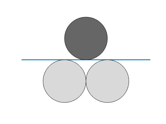
Theorem 1.1 can also be reformulated in the setup of shallow fully-connected feedforward ANNs with multi-dimensional input layers and multi-dimensional hidden layers with the ReLU activation for all except of one neuron on the hidden layer and the identity activation for the remaining neuron on the hidden layer. This reformulation of Theorem 1.1 is precisely the subject of the next result in Theorem 1.2 below. We also refer to Figure 1 for a graphical visualization illustrating the in Theorem 1.2 employed ANN architectures with neurons on the input layer and neurons on the hidden layer.
Theorem 1.2 (Existence of minimizer – fully-connected feedforward ANNs).
Let , , let and be continuous, assume that is a bounded and convex set, for every let satisfy for all that
| (4) |
and let satisfy for all that . Then there exists such that .
Theorem 1.1 and Theorem 1.2 are both direct consequences of the more general result in Theorem 1.3 below (which covers more general supports of the probability distribution of the input data of the consider learning problem and also covers a general class of loss functions instead of only the standard mean square loss). In this regard, we note that the set of the realization functions of shallow fully-connected feedforward ANNs with neurons on the input layer, with neurons on the hidden layer, with the ReLU activation for neurons on the hidden layer, and with the identity activation for the remaining neuron on the hidden layer (see Figure 1) coincides with the set of the realization functions of shallow residual ReLU ANNs with neurons on the input layer, with neurons on the hidden layer, and with a skip-connection from the input layer to the output layer.
Theorem 1.1 and Theorem 1.2 somehow employ a vectorized description of ANNs in the sense that every real vector represents an ANN whose realization function is . In our more general Theorem 1.3 and in our later arguments, we represent ANNs in a more structurized way (see 5 below). More specifically, in the following we describe every ANN by a quadrupel consisting
-
•
of a matrix (weight matrix to describe the linear part in the affine transformation from the -dimensional input layer to the -dimensional hidden layer),
-
•
of a vector (bias vector to the additive part in the affine transformation from the -dimensional input layer to the -dimensional hidden layer),
-
•
of a matrix (weight matrix to describe the linear part in the affine transformation from the -dimensional hidden layer to the -dimensional output layer), and
-
•
of a scalar (bias to describe the additive part in the affine transformation from the -dimensional hidden layer to the -dimensional output layer).
Moreover, for every we write . We let
| (5) |
and call a network configuration and the parametrization class. We often refer to a configuration of a neural network as the (neural) network . A configuration describes a function via
| (6) |
where denotes the scalar product. We call realization function or response of the network .
Note that in general the response of a network is a continuous and piecewise affine function from to . We conceive as a parametrization of a class of potential response functions in a minimization problem. More explicitly, let be a finite measure on the Borel sets of , let be the support of , and let be a product measurable function, the loss function. We aim to minimize the error
| (7) |
over all for a given and we let
| (8) |
the minimal error with neurons in the hidden layer. We stress that if there does not exist a neural network satisfying then every sequence of networks satisfying diverges to infinity.
The class of responses that is considered in this article clearly contains all responses of shallow ANNs having only ReLU neurons in the hidden layer and no linear neuron. Conversely since an affine function can be represented as the response of two ReLU neurons, is also contained in the class of responses of shallow ANNs using neurons in the hidden layer that all apply the ReLU activation function. If is compactly supported, then the -restricted responses in even can be expressed by shallow ReLU networks with neurons.
Overparametrized networks in the setting of empirical risk minimization (more ReLU neurons than data points to fit) are often able to perfectly interpolate the data such that there exists a network configuration achieving zero error and, thus, a global minimum in the search space . However, for general measures not necessarily consisting of a finite number of Dirac measures or consisting of a finite number of Dirac measures but in the practically more realistic underparametrized regime, the literature on the existence of global minima is very limited and we refer the reader to [JR22, Theorem 1.1] for a result in the setting of shallow ReLU ANNs with one-dimensional input. See also [KKV03] for a similar result concerning the existence of global minima in the regression task of approximating functions in the space with shallow ANNs using heavyside activation. We also refer to [Sin70] for a general introduction into best approximators in normed spaces. We also point, e.g., to [CB18, DZPS19, DLL+19, CB20, Woj20] and the references therein for sophisticated convergence analysis for GD optimization methods in such overparametrized regimes.
A good literature review regarding the loss landscape in neural network training can be found in [EMWW20]. For statements about the existence of and convergence to non-optimal local minima in the training of (shallow) networks we refer the reader, e.g., to [SCP16, SS18, VBB19, CK22, GW22, IJR22].
In this article, we show under mild assumptions on the measure and the loss function that there exists a global minimum in the loss landscape. We suggest a kind of closure of the search space and, in a second step, show that the additional artificial responses are not optimal in the minimization problem. We state the main result of this article.
Theorem 1.3 (Existence of minimizers – general loss functions and fully-connected feedforward ANNs).
Assume that is compact, assume that has a continuous Lebesgue density , assume that for every hyperplane intersecting the interior of the convex hull of there is an element with , and assume that the loss function satisfies the following assumptions:
-
(i)
(Continuity in the first argument) For every it holds that is continuous.
-
(ii)
(Strict convexity in the second argument) For all it holds that is strictly convex and attains its minimum.
Then it holds for every that there exists an optimal network with .
Theorem 1.3 is an immediate consequence of 3.3 below. We stress that the statement of 3.3 is stronger in the sense that it even shows that in many situations the newly added functions to the extended target space perform strictly worse than the representable responses.
Example 1.4 (Regression problem).
Let be as in Theorem 1.3, let be continuous, and let be a strictly convex function that attains its minimum. Then the function given by
| (9) |
for all , satisfies the assumptions of Theorem 1.3 and Theorem 1.3 allows us to conclude that the infimum
| (10) |
is attained for a network .
2. Generalized response of neural networks
We will work with more intuitive geometric descriptions of realization functions of networks . We slightly modify the ideas given in [DK22b] and later introduce the notion of a generalized response. Then, we show in Proposition 2.4 that, in a general approximation problem, there always exists a generalized response that solves the minimization task at least as good as the class .
We call a network non-degenerate iff for all we have . For a non-degenerate network , we say that the neuron has
-
•
normal ,
-
•
offset , and
-
•
kink .
Moreover, we call the affine mapping given by
| (11) |
affine background. We call with , , and the affine function the effective tuple of and write for the set of all effective tuples using ReLU neurons.
First, we note that the response of a non-degenerate ANN can be represented in terms of its effective tuple:
| (12) |
With slight misuse of notation we also write
| (13) |
and Although the tuple does not uniquely describe a neural network, it describes a response function uniquely and thus we will speak of the neural network with effective tuple .
We stress that also the response of a degenerate network can be described as response associated to an effective tuple. Indeed, for every with the respective neuron has a constant contribution . Now, one can choose an arbitrary normal and offset , set the kink equal to zero () and add the constant to the affine background . Repeating this procedure for every such neuron we get an effective tuple that satisfies . Conversely, for every effective tuple , the mapping is the response of an appropriate network . In fact, for , one can choose , and and gets that for all
| (14) |
Analogously, one can choose , , and such that for all
| (15) |
This entails that
| (16) |
and the infimum is attained iff there is a network for which the infimum in (8) is attained.
For an effective tuple , we say that the th ReLU neuron has the breakline
| (17) |
and we call
| (18) |
the domain of activity of the th ReLU neuron. By construction, we have
| (19) |
Outside the breaklines the function is differentiable with
| (20) |
Note that for each summand along the breakline the difference of the differential on and equals (which is also true for the response function provided that it is differentiable in the reference points and there does not exist a second neuron having the same breakline ).
For a better understanding of the optimization problem discussed in this article it makes sense to view the set of responses as a subset of the locally convex vector space of locally integrable functions. Then the set of response functions is not closed and the main task of this article is to show that functions that can be approached by functions from but are itself no response functions will provide larger errors than the response functions.
We now extend the family of response functions.
Definition 2.1.
We call a function a generalized response (generalized realization function) if it admits the following representation: there are , a tuple of open half-spaces of with pairwise distinct boundaries , a vector , an affine mapping , vectors , and reals such that
-
(i)
it holds for all that
(21) and
-
(ii)
it holds for all with that
(22)
We will represent generalized responses as in 21, we call the active half-spaces of the response, and we call the multiplicities of the half-spaces . The minimal number that can be achieved in such a representation is called the dimension of . For every we denote by the family of all generalized responses of dimension or smaller. We call a generalized response simple if it is continuous which means that all mutliplicities can be chosen equal to one. A response is called strict at dimension if the response has dimension or is discontinuous. We denote by the responses in that are strict at dimension .
Remark 2.2.
Note that the sets and agree.
In this section, we work with a general measure which may have unbounded support. The assumptions on are stated in the next definition.
Definition 2.3.
-
(i)
An element of a hyperplane is called -regular if and , where is an open half-space with .
-
(ii)
A measure is called nice if all hyperplanes have -measure zero and if for every open half-space with the set of -regular points cannot be covered by finitely many hyperplanes different from .
Next, we will show that under quite weak assumptions there exist generalized responses of dimension or smaller that achieve an error of at most .
Proposition 2.4.
Assume that is a nice measure on a closed subset of and assume that the loss function is measurable and satisfies the following assumptions:
-
(i)
(Lower-semincontinuity in the second argument) For all , we have
(23) -
(ii)
(Unbounded in the second argument) For all we have
(24)
Let with . Then there exists a generalized response which satisfies
| (25) |
Furthermore, if , then the infimum
| (26) |
is attained on .
Proof.
Let be a sequence of generalized responses in that satisfies
| (27) |
We use the representations as in 21 and write
| (28) |
Moreover, denote by and the quantities with and by the respective multiplicities.
1. Step: Choosing an appropriate subsequence.
Since for all we can choose a subsequence such that there exists with for all . For ease of notation we will assume that this is the case for the full sequence. With the same argument we can assume without loss of generality that there exists such that for all we have .
Moreover, after possibly thinning the sequence again we can assure that for all we have convergence in the compact space and in the two point compactification . We assign each an asymptotic active area given by
| (29) |
which is degenerate in the case where .
We denote by the respective breakline . Even if, for every , the original breaklines are pairwise distinct, this might not be true for the limiting ones. In particular, there may be several ’s for which the asymptotic active areas may be on opposite sides of the same breakline. In that case we choose one side and replace for each with asymptotic active area on the opposite side its contribution in the representation 21 from to
| (30) |
which agrees with the former term outside the breakline (which is a zero set). This means we replace , , and by , , and , respectively, and adjust the respective affine background accordingly. Thus we can assume without loss of generality that all asymptotic active areas sharing the same breakline are on the same side.
We use the asymptotic active areas to partition the space: let denote the collection of all subsets for which the set
| (31) |
satisfies . We note that the sets , , are non-empty, open, and pairwise disjoint and their union has full -measure since
| (32) |
Moreover, for every and every compact set with one has from a -dependent onwards that the generalized response satisfies for all that
| (33) |
where
| (34) |
Let . Next, we show that along an appropriate subsequence, we have convergence of in . First assume that along a subsequence one has that converges to . For ease of notation we assume without loss of generality that . We let
| (35) |
For every with , is a hyperplane which can be parametrized by taking a normal and the respective offset. As above we can argue that along an appropriate subsequence (which is again assumed to be the whole sequence) one has convergence of the normals in and of the offsets in . We denote by the hyperplane being associated to the limiting normal and offset (which is assumed to be the empty set in the case where the offsets do not converge in ). Since the norm of the gradient tends to infinity we get that for every one has and, hence, . Consequently, Fatou implies that
| (36) |
contradicting the asymptotic optimality of . We showed that the sequence is precompact and by switching to an appropriate subsequence we can guarantee that the limit exists.
Similarly we show that along an appropriate subsequence converges to a value . Suppose this were not the case, then there were a subsequence along which (again we assume for ease of notation that this is the case along the full sequence). Then for every , and we argue as above that this contradicts the optimality of . Consequently, we have for an appropriately thinned sequence on a compact set uniform convergence
| (37) |
Since has full -measure we get with the lower semicontinuity of in the second argument and Fatou’s lemma that for every measurable function satisfying for each , that
| (38) |
we have
| (39) |
Step 2: may be chosen as a generalized response of dimension or smaller.
We call a summand degenerate if or has -measure zero. We omit every degenerate summand in the sense that we set and for all and note that by adjusting the affine background appropriately we still have validity of 37 with the same limit on all relevant cells and, in particular, -almost everywhere.
Let now be a non-degenerate summand. Since is nice there exists a -regular point that is not in , where . We let
| (40) |
Since we get that the cell has strictly positive -measure so that . Analogously, entails that . (Note that and are just the cells that lie on the opposite sides of the hyperplane at .) We thus get that
| (41) |
where the definitions of and do not depend on the choice of . Analogously,
| (42) |
Now for general , we have
| (43) |
Since and converge to and , respectively, we have that and converge and there is an appropriate affine function such that for all and
| (44) |
So far, we have only used the definition of on and we now assume that is chosen in such a way that the latter identity holds for all (by possibly changing the definition on a -nullset). We still need to show that is a generalized response of dimension or smaller.
Every active area that is the asymptotic active area of a single non-degenerate summand with is assigned the multiplicity one. All other non-degenerate active areas get multiplicity two. Then the overall multiplicity (the sum of the individual multiplicities) is smaller or equal to the dimension . To see this recall that every active area that is the asymptotic area of more than one summand or one summand of multiplicity two also contributed at least two to the multiplicity of the approximating responses. All degenerate summands do not contribute at all although they contribute to the approximating responses.
It remains to show that is indeed a generalized response with the active areas having the above multiplicities. For this it remains to show continuity of for all with assigned multiplicity one. Suppose that the th summand is the unique summand that contributes to such an . Then and . Moreover, one has
| (45) |
which entails that, in particular, is a multiple of . Both latter vectors converge which also entails that the limit is a multiple of . To show that
| (46) |
is satisfied it thus suffices to verify that one point of the set on the left-hand side lies also in the set on the right-hand side. This is indeed the case since is in the set on the left-hand side and
| (47) |
where we used that satisfies by assumption .
Step 3: The infimum over all strict responses is attained.
We suppose that is a sequence of strict generalized responses satisfying
| (48) |
Then we can find a subsequence of responses in or a subsequence of responses where at least one active area has multiplicity two. In the former case the response constructed above is a generalized response of dimension or lower which is strict at dimension . Conversely, in the latter case the construction from above will lead to a generalized response that has at least one active area with multiplicity two which, in turn, implies that is either of dimension strictly smaller than or is discontinuous. ∎
Remark 2.5 (Asymptotic ANN representations for generalized responses).
In this remark, we show that every generalized response of dimension is, on , the limit of ANN responses of ANNs in .
Let , and and set
| (49) |
We will show that the generalized response is on the limit of the response of two ReLU neurons. For every , the following function
| (50) |
is the response of a shallow ReLU ANN with two hidden ReLU neurons. Now note that for all one has so that
| (51) |
Analogously, . Consequently, for these one has for large that
| (52) |
Conversely, for all one has so that analogously to above and . Consequently, for these one has for large that
| (53) |
We thus represented as asymptotic response of a ReLU ANN with two hidden neurons.
For a generalized response one replaces every term of multiplicity two (see (21)) by two ReLU neurons exactly as above. Moreover, the terms with multiplicity one are responses of ANNs with one ReLU neuron.
3. Discontinuous responses are not optimal
In this section, we show that generalized responses that contain discontinuities are not optimal in the minimization task for a loss function that is continuous in the first argument. This proves Theorem 1.3 since all continuous generalized responses can be represented by shallow networks.
In the proofs we will make use of the following properties of the loss functions under consideration.
Lemma 3.1.
Let be a function satisfying the following assumptions:
-
(i)
(Continuity in the first argument) For every it holds that is continuous.
-
(ii)
(Strict convexity in the second argument) For all it holds that is strictly convex and attains its minimum.
Then
-
(I)
it holds that is continuous,
-
(II)
it holds for every compact that the function is continuous with to the supremum norm,
-
(III)
it holds that there exists a unique which satisfies for every that
(54) and
-
(IV)
it holds that and are continuous.
Proof.
Regarding (I): The proof can, e.g, be found in [Roc70, Theorem 10.7].
Regarding (II): The proof can, e.g., be found in [Roc70, Theorem 10.8].
Regarding (III): The existence and uniqueness of is an immediate consequence of property (ii).
Regarding (IV): We show continuity of and . Let and choose with . Now, there exists a neighbourhood of such that
| (55) |
for all and with the strict convexity of we get for all
| (56) |
Hence, for all we have and the continuity of follows from (II). Moreover, since and where arbitrary we also have continuity of . ∎
Clearly, we have that
| (57) |
so that the minimization task reduces to finding a good approximation for on the support of . If is the response of an ANN for , then minimizes the error . If is not representable by a network using ReLU neurons then one expects the minimal error to strictly decrease after adding a ReLU neuron to the network structure, i.e., . This is true in many situations (see 3.5) but there exist counterexamples to this intuition (see 3.7).
We note that the set of generalized responses is invariant under right applications of affine transformations that are one-to-one.
Lemma 3.2.
Let , let a mapping, and let be an affine mapping that is injective. Then the following properties hold for iff the corresponding properties hold for :
-
(i)
-
(ii)
-
(iii)
is simple.
Proof.
Suppose that is represented as in 21 with the active areas being for all
| (58) |
We represent the affine function as with and . Then obviously
| (59) |
with , , , and
| (60) |
where denotes the transpose of a vector or a matrix. Clearly, continuity of the summands is preserved and, hence, one can choose the same multiplicities. Therefore, is again in and it is even strict at dimension or simple if this is the case for . Applying the inverse affine transform we also obtain equivalence of the properties. ∎
We are now in the position to prove the main statement of this article, Theorem 1.3. It is an immediate consequence of the following stronger result.
Proposition 3.3.
Suppose that the assumptions of Theorem 1.3 are satisfied. Let . Then there exists an optimal network with
| (61) |
If additionally and , then one has that
| (62) |
Proof.
We can assume without loss of generality that . First we verify the assumptions of 2.4 in order to conclude that there are generalized responses of dimension for which
| (63) |
We verify that is a nice measure: In fact, since has Lebesgue-density , we have for all hyperplanes . Moreover, for every half-space with we have that intersects the interior of the convex hull of so that there exists a point with . Since is an open set, cannot be covered by finitely many hyperplanes different from . Moreover, since for all the function is strictly convex and attains its minimum we clearly have for fixed continuity of and
We prove the remaining statements via induction over the dimension . If , all generalized responses of dimension are representable by a neural network and we are done. Now let and suppose that is the best strict generalized response at dimension . It suffices to show that one of the following two cases enters: one has
| (64) |
or
| (65) |
Indeed, then in the case that (65) does not hold we have as consequence of (64)
| (66) |
and the induction hypothesis entails that so that and . Thus, an optimal simple response of dimension (which exists by induction hypothesis) is also optimal when taking the minimum over all generalized responses of dimension or smaller. Conversely, if (65) holds, an optimal generalized response (which exists by Proposition 2.4) is simple so that, in particular, . This shows that there always exists an optimal simple response. Moreover, it also follows that in the case where , either of the properties (64) and (65) entail property (62).
Suppose that is given by
| (67) |
with being the pairwise different activation areas and being the respective multiplicities. Note that has to be discontinuous, because otherwise is of dimension strictly smaller than d and 64 holds. Therefore, we can assume without loss of generality that and
| (68) |
(otherwise we reorder the terms appropriately).
If does not intersect the interior of , then one can replace the term by or without changing the error on . By doing so the new response has dimension or smaller. Thus, we get that
| (69) |
Now suppose that intersects the interior of . We prove that is not an optimal response in by constructing a better response. To see this we apply an appropriate affine transformation on the coordinate mapping. For an invertible matrix and a vector we consider the invertible affine mapping
| (70) |
By Lemma 3.2 the (strict) generalized responses are invariant under right applications of bijective affine transformations so that is an optimal strict generalized response for the loss function given by .
Now we distinguish two cases. In line with the notation from before we denote by and the unique values for which . First suppose that and are linearly independent. We choose a basis of such that , , and for . This can be achieved by first choosing an arbitrary basis of the space of vectors being orthogonal to , secondly choosing a vector that is orthogonal to but not to which is possible since and are linearly independent and finally letting .
We denote by the matrix consisting of the basis vectors and choose so that
| (71) |
The latter is feasible since the expression on the left hand side only depends on the choice of and the expression on the right hand side only on the coordinates .
As is straight-forward to verify the respective response has as th active area and on the th summand in the respective representation of is
| (72) |
Altogether the previous computations show that we can assume without loss of generality that the considered strict generalized response has as active area with being perpendicular to the first unit vector and being zero.
We compare the performance of the response with the -indexed family of generalized responses of dimension or smaller given by
| (73) |
where
| (74) |
Let
| (75) |
and similarly and note that
| (76) |
where
| (77) |
For denote by the set
| the segment has distance greater or equal to to every () | |||
It is straight-forward to verify that is closed and due to the compactness of also compact. Moreover,
| (78) |
We have
| (79) | ||||
where . In dependence on we partition in two sets
| (80) |
We note that is continuous on as consequence of the continuity of (see Lemma 3.1) and the particular choice of . Moreover, for sufficiently large (depending on ), . Using that continuous functions are uniformly continuous on compacts, that is uniformly bounded and the Lebesgue measure of is of order we conclude that in terms of
| (81) |
as . Moreover, for every one has
| (82) |
We represent in terms of the measure , the strictly convex function
| (83) |
and its secant that equals in the boundary points and is linear in between. One has
| (84) |
with strict inequality in the case where (due to strict convexity). Consequently, we get with LABEL:eq578 that
| (85) |
To analyze the contribution of the integrals on we note that by uniform boundedness of over all and one has existence of a constant not depending on and such that
| (86) |
where is the -dimensional Hausdorff measure of the set . By choosing arbitrarily small one can make arbitrarily small and with a diagonalization argument we obtain with (79) and (85) that
| (87) |
Now there exists with and by continuity of we can choose such that, additionally, . By continuity we thus get that
| (88) |
and, consequently, there exists such that the generalized response of dimension or smaller has a strictly smaller error than . Hence, it has to be simple.
It remains to treat the case where and are linearly dependent. In that case we choose with , we extend to an orthonormal basis of and denote by the matrix formed by the vectors . Moreover, choose and set . Then the response has as th activation area and on the th summand in the respective representation of is
| (89) |
where since otherwise we would have that
| (90) |
We showed that in the remaining case we can assume without loss of generality that , for an and .
In analogy to above we compare the response with the -indexed family of responses given by
| (91) |
where
| (92) |
We use and as before, see 75, and note that agrees with for all with . In analogy to above, we conclude that
| (93) |
where . As above we split the domain of integration into the two sets and . Now in terms of
| (94) |
we get by using the uniform continuity of on and the fact that as that
| (95) |
By strict convexity of , we get that . With the same arguments as in the first case one obtains that
| (96) |
so that there exists a response with strictly smaller error than and the proof is finished. ∎
Example 3.4.
If there exists a hyperplane with for all such that intersects the convex hull of the conclusion of Theorem 1.3 is in general not true. Consider a continuous function that satisfies for all and for all . Now, let and be the measure on with continuous Lebesgue density
| (97) |
Then, we have on . Note that
| (98) |
is a strict generalized response of dimension with . Conversely, there does not exist a network (for arbitrary ) with . In particular, assume that there exist and with . Then, every breakline that intersects the interior of contains an uncountable set of points with and for all such points the function is constant in a neighborhood of . Therefore, the collective response of the neurons with breakline has to be constant and we can without loss of generality assume that all ReLU neurons have the breakline . Moreover, since it holds that for all with and for all with . This contradicts the continuity of .
Thus, there does not exist a global minimum in the loss landscape (for arbitrary ) and, in order to solve the minimization task iteratively, the sequence of networks returned by a gradient based algorithm have unbounded parameters.
For a thorough investigation of the non-existence of global minima in the approximation of discontinuous target functions , see [GJL22].
Next, we show that in many situations if the class of network responses is not able to produce the function defined in Lemma 3.1 the minimal error strictly decreases after adding a ReLU neuron to the network structure.
Proposition 3.5.
Let , assume that is a compact set, assume there exists with , assume for every that the function is convex,
-
(i)
assume for every compact there exists such that for all , that
(99) -
(ii)
assume for every affine function that the set
(100) is a Lebesgue nullset,
and assume that there exist no neural network satisfying for -almost all that
| (101) |
Then
| (102) |
Remark 3.6.
We compare the assumptions of 3.5 with those of Theorem 1.3. In 3.5 we explicitly assume the existence of an optimal network and relax the continuity assumption on in the first component and the strict convexity assumption on in the second component. On the other hand, we introduce assumptions on the smoothness of in the second component. Under the assumptions of Theorem 1.3, condition (i) of 3.5 is satisfied (cf. [Roc70, Thm. 10.6]) and we can apply the latter proposition if additionally condition (ii) is satisfied. In that case, the statement of 3.5 can be rewritten as follows: if , then there exists a neural network with for all .
Proof of 3.5.
Let be a network with . For , consider the function
| (103) |
If then we have for all , that
| (104) |
and taking the derivative with respect to at yields
| (105) |
where is uniformly bounded and well-defined outside a Lebesgue nullset. Indeed, since is piecewise affine there exists a finite number of affine functions such that the set of points for which is not -differential in is contained in
| (106) |
which by (ii) is a nullset. Moreover, the boundedness of the derivative follows from the Lipschitz continuity of in the second argument, see (i). We let
| (107) |
and note that the space of all continuous functions satisfying
| (108) |
is linear and closed under convergence in (endowed with supremum norm). We showed that contains all functions of the form and it is standard to deduce that contains all polynomials and, using the Stone-Weierstrass theorem, thus all continuous functions. By the Riesz–Markov–Kakutani representation theorem, the measure is the zero-measure and is zero except for -nullsets. Note that , -almost everywhere, and hence , -almost everywhere. Using the convexity of we get , -almost everywhere. ∎
In the next example, we show that the conclusion of Proposition 3.5 is in general false if condition (ii) is not satisfied. We note that the loss function in the example is not strictly convex but the statements of Lemma 3.1 still hold in this case.
Example 3.7.
Consider the following regression problem. Let , , be the Lebesgue measure on the interval and where
| (109) |
Note that and
| (110) |
so that is the response of a network using three ReLU neurons and . We show that for we have
| (111) |
i.e. the best regression function in the set of response functions for networks having ReLU neurons is the zero function although is not the zero function. This shows that the conclusion of 3.5 is in general false if Assumption (ii) is not satisfied.
Denote by the function
| (112) |
where is the set of all closed intervals that are subsets of . We show that for we have for all networks .
Let . Then is continuous and satisfies
| (113) |
for with .
First, we assume that and . We fix and derive a lower bound for over all feasible choices of and . We start with the case . Note that the choice , yields a better result than all networks with . Therefore we can restrict the optimization task to networks satisfying For we show that, indeed, the optimal choice for the approximation of on the right-hand side of the -axis is , . If and then
| (114) |
where with . Conversely, if then . We consider two cases. If then . Thus, so that for we get . If then . In that case, corresponds to the area of two triangles with slope and baselines that add to . This is minimized by two congruent triangles so that
| (115) |
Thus, for we get and the optimal choice is , .
It remains to consider the case . In this case the choice is clearly suboptimal and for we get . The above calculations show that
| (116) |
so that for we have . If the choice is suboptimal and in the case where is not the optimal choice it is easy to see that actually , is the best choice. In that case
| (117) |
In conclusion, in all of the above cases we get for that .
Next, we consider the case . Set . Choosing or is clearly suboptimal. For and note that . Analogously to the case we get
| (118) |
so that for
| (119) |
Now, if and then the above calculations imply that . Using the symmetry of the problem we showed that for all networks satisfying we have that
| (120) |
Using again the symmetry, we are therefore left with considering the case . We can cleary focus on the case and . Note that one can use the above arguments in order to show that
| (121) |
If we thus get
| (122) |
On the other hand, so that, for , we have . Conversely, if we get
| (123) |
and for and we clearly have . For we get
| (124) |
Now for we get
| (125) |
and for we get that . If then
| (126) |
Thus, if have and the proof of the assertion is finished.
Acknowledgements
We gratefully acknowledge the Cluster of Excellence EXC 2044-390685587, Mathematics Münster: Dynamics-Geometry-Structure funded by the Deutsche Forschungsgemeinschaft (DFG, German Research Foundation). This work has been partially funded by the Deutsche Forschungsgemeinschaft (DFG, German Research Foundation) – SFB 1283/2 2021 – 317210226.
References
- [AB09] H. Attouch and J. Bolte. On the convergence of the proximal algorithm for nonsmooth functions involving analytic features. Mathematical Programming, 116(1):5–16, 2009.
- [AMA05] P.-A. Absil, R. Mahony, and B. Andrews. Convergence of the iterates of descent methods for analytic cost functions. SIAM Journal on Optimization, 16(2):531–547, 2005.
- [BDL07] J. Bolte, A. Daniilidis, and A. Lewis. The Łojasiewicz inequality for nonsmooth subanalytic functions with applications to subgradient dynamical systems. SIAM Journal on Optimization, 17(4):1205–1223, 2007.
- [CB18] L. Chizat and F. Bach. On the global convergence of gradient descent for over-parameterized models using optimal transport. arXiv:1805.09545, 2018.
- [CB20] L. Chizat and F. Bach. Implicit Bias of Gradient Descent for Wide Two-layer Neural Networks Trained with the Logistic Loss. arXiv:2002.04486, 2020.
- [CK22] C. Christof and J. Kowalczyk. On the omnipresence of spurious local minima in certain neural network training problems. arXiv:2202.12262, 2022.
- [DDKL20] D. Davis, D. Drusvyatskiy, S. Kakade, and J. D. Lee. Stochastic subgradient method converges on tame functions. Found. Comput. Math., 20(1):119–154, 2020.
- [DK21] S. Dereich and S. Kassing. Convergence of stochastic gradient descent schemes for Łojasiewicz-landscapes. arXiv:2102.09385, 2021.
- [DK22a] S. Dereich and S. Kassing. Cooling down stochastic differential equations: Almost sure convergence. Stochastic Processes and their Applications, 152:289–311, 2022.
- [DK22b] S. Dereich and S. Kassing. On minimal representations of shallow ReLU networks. Neural Networks, 148:121–128, 2022.
- [DLL+19] S. S. Du, J. D. Lee, H. Li, L. Wang, and X. Zhai. Gradient descent finds global minima of deep neural networks. arXiv:1811.03804, 2019.
- [DZPS19] S. S. Du, X. Zhai, B. Poczos, and A. Singh. Gradient Descent Provably Optimizes Over-parameterized Neural Networks. arXiv:1810.02054, 2019.
- [EJRW21] S. Eberle, A. Jentzen, A. Riekert, and G. S. Weiss. Existence, uniqueness, and convergence rates for gradient flows in the training of artificial neural networks with ReLU activation. To appear in the Electronic Research Archive, arXiv:2108.08106, 2021.
- [EMWW20] W. E, C. Ma, S. Wojtowytsch, and L. Wu. Towards a mathematical understanding of neural network-based machine learning: what we know and what we don’t. arXiv:2009.10713, 2020.
- [GJL22] D. Gallon, A. Jentzen, and F. Lindner. Blow up phenomena for gradient descent optimization methods in the training of artificial neural networks. arXiv:2211.15641, 2022.
- [GW22] R. Gentile and G. Welper. Approximation results for Gradient Descent trained Shallow Neural Networks in 1d. arXiv:2209.08399, 2022.
- [IJR22] S. Ibragimov, A. Jentzen, and A. Riekert. Convergence to good non-optimal critical points in the training of neural networks: Gradient descent optimization with one random initialization overcomes all bad non-global local minima with high probability. arXiv:2212.13111, 2022.
- [JR22] A. Jentzen and A. Riekert. On the existence of global minima and convergence analyses for gradient descent methods in the training of deep neural networks. Journal of Machine Learning, 1(2):141–246, 2022.
- [KKV03] P. C. Kainen, V. Kurková, and A. Vogt. Best approximation by linear combinations of characteristic functions of half-spaces. Journal of Approximation Theory, 122(2):151–159, 2003.
- [Łoj63] S. Łojasiewicz. Une propriété topologique des sous-ensembles analytiques réels. Les équations aux dérivées partielles, 117:87–89, 1963.
- [Łoj65] S. Łojasiewicz. Ensembles semi-analytiques. Lectures Notes IHES (Bures-sur-Yvette), 1965.
- [Łoj84] S. Łojasiewicz. Sur les trajectoires du gradient d’une fonction analytique. Seminari di geometria, 1982/1983:115–117, 1984.
- [MHKC20] P. Mertikopoulos, N. Hallak, A. Kavis, and V. Cevher. On the almost sure convergence of stochastic gradient descent in non-convex problems. In Advances in Neural Information Processing Systems, volume 33, pages 1117–1128, 2020.
- [PRV21] P. Petersen, M. Raslan, and F. Voigtlaender. Topological properties of the set of functions generated by neural networks of fixed size. Found. Comput. Math., 21(2):375–444, 2021.
- [Roc70] R. T. Rockafellar. Convex Analysis, volume 36. Princeton University Press, 1970.
- [SCP16] G. Swirszcz, W. M. Czarnecki, and R. Pascanu. Local minima in training of neural networks. arXiv:1611.06310, 2016.
- [Sin70] I. Singer. Best Approximation in Normed Linear Spaces by Elements of Linear Subspaces. Springer, 1970.
- [SS18] I. Safran and O. Shamir. Spurious local minima are common in two-layer ReLU neural networks. In International conference on machine learning, pages 4433–4441. PMLR, 2018.
- [Tad15] V. B. Tadić. Convergence and convergence rate of stochastic gradient search in the case of multiple and non-isolated extrema. Stochastic Processes and their Applications, 125(5):1715–1755, 2015.
- [VBB19] L. Venturi, A. S. Bandeira, and J. Bruna. Spurious valleys in one-hidden-layer neural network optimization landscapes. Journal of Machine Learning Research, 20(133):1–34, 2019.
- [Woj20] S. Wojtowytsch. On the Convergence of Gradient Descent Training for Two-layer ReLU-networks in the Mean Field Regime. arXiv:2005.13530, 2020.