LIO-PPF: Fast LiDAR-Inertial Odometry via
Incremental Plane Pre-Fitting and Skeleton Tracking

Abstract

As a crucial infrastructure of intelligent mobile robots, LiDAR-Inertial odometry (LIO) provides the basic capability of state estimation by tracking LiDAR scans. The high-accuracy tracking generally involves the kNN search, which is used with minimizing the point-to-plane distance. The cost for this, however, is maintaining a large local map and performing kNN plane fit for each point. In this work, we reduce both time and space complexity of LIO by saving these unnecessary costs. Technically, we design a plane pre-fitting (PPF) pipeline to track the basic skeleton of the 3D scene. In PPF, planes are not fitted individually for each scan, let alone for each point, but are updated incrementally as the scene ‘flows’. Unlike kNN, the PPF is more robust to noisy and non-strict planes with our iterative Principal Component Analyse (iPCA) refinement. Moreover, a simple yet effective sandwich layer is introduced to eliminate false point-to-plane matches. Our method was extensively tested on a total number of 22 sequences across 5 open datasets, and evaluated in 3 existing state-of-the-art LIO systems. By contrast, LIO-PPF can consume only 36% of the original local map size to achieve up to 4$\times$ faster residual computing and 1.92$\times$ overall FPS, while maintaining the same level of accuracy. We fully open source our implementation at https://github.com/xingyuuchen/LIO-PPF.

I Introduction

Estimating the ego-motion and meanwhile building the 3D map of the environment (SLAM) is a fundamental tool for intelligent mobile robots, which is requisite for many downstream applications such as route planning and obstacle avoidance. Among all the sensors, 3D LiDARs provide accurate, long-range and light-invariant detection of the environment; Inertial Measurement Unit (IMU) measures the robot’s movement at high frequency and can therefore compensate each LiDAR point’s motion. As a result, these two sensors are widely deployed together on mobile robots.

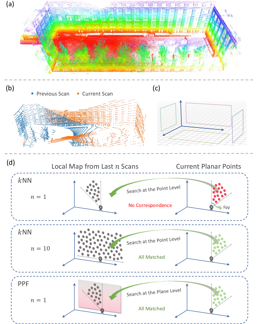
Figure 1: (a) The reconstructed scene. (b) Two consecutive scans of (a) under rapid rotations. (c) Large planes across the scans form the basic skeleton of the scene and reveal its overall geometry structure. (d) A large local map is needed by kNN otherwise most points can’t find neighbors to fit planes. While we use the basic skeleton to represent the scene for point matching. The search field is enlarged to plane level with no kNN search required.

Though deep learning methods have made great progress and sometimes outperform traditional LIO, not to mention the poor generalizability across different datasets, the high power of modern GPUs is still too expensive, which is not applicable to most battery-powered mobile agents. Moreover, in typical intelligent robots, LIO runs only at the low level of the overall system, where high-level tasks (e.g. route planning) can take up most computational resources. Therefore, all infrastructures should be guaranteed to run robustly and efficiently. For this, this paper focuses on reducing both the time and space complexity of the low-level LIO systems.

Modern real-time LIO solves the ego-motion by registering LiDAR scans [1, 2, 3, 4, 5, 6]. The registration is based on the geometry constraints, i.e. point-to-plane distance [4, 2, 3] (and sometimes point-to-edge distance [5, 6]). To match each point to its corresponding plane, the nearest-neighbor (NN) search is performed, and the local plane patch is then fitted from k (4$\sim$5) NN. One strategy is to register consecutive scans [1], namely, scan-to-scan. Though fast, this strategy can easily end up with few matched points caused by small FoV or aggressive rotational maneuvers, e.g. Fig. 1d top. Therefore, recent methods registered the latest LiDAR scan to the local map [2, 3, 4, 5, 6], which consists of several selected scans transformed to the same coordinate system, thereby providing more points for kNN search. This ensures sufficient matched points and high accuracy. However, maintaining a large local map, performing kNN search and plane fitting for each point sacrifice both memory and efficiency.

In this paper, compared to lazily fitting the plane after searching kNN for each point, we adopt a more active plane pre-fitting manner. This idea stems from two un-necessities:

1) Unnecessary kNN. Current LiDAR scan tracking [1, 2, 3, 4, 5, 6] search kNN for every single point to fit a plane, assuming that spatially close points are from the same plane. However, the condition is too strict, i.e., spatially distant points can also belong to the same plane, e.g. long walls. In other words, the kNN strategy neglects the fact that planes are not always in small local areas. For large planes, most kNN searches are redundant as they turn out to fit the same plane. Meanwhile, points from successive LiDAR scans often come from different parts of the same large plane, i.e., they share the same high-level large planar object. This gives us a hint: If searching happens in the high-level feature plane space, the expensive costs from kNN could naturally be saved.

2) Unnecessary large local map. If preserving only a few scans in the local map, NN might be far away and thus likely to belong to other objects, resulting in the kNN being inaccurate to fit the matching plane. Hence, the local map is enlarged to guarantee sufficient close-enough point-to-kNN correspondences [5, 6, 7], see Fig. 1d. However, we note that: Even with only one scan kept in the local map, the absence of close NN $\neq$ the absence of plane match. E.g., in Fig. 1b, most orange wall points failed to find close NN on the long wall, the plane of which, however, can be easily pre-fitted from the points within one single previous scan (blue points). Again, this gives us a hint: If searching happens in the high-level feature plane space, one single previous scan is enough to provide adequate point-to-plane matches.

In summary, we make the following contributions:

• We propose to represent the scene by its basic skeleton for point matching, which is done via plane pre-fitting (PPF) across LiDAR scans. We demonstrate (i) PPF can naturally downsize the local map and eliminate most of the redundant kNN searches and plane fittings; (ii) the un-robustness of kNN to noisy and non-strict planes.

• In PPF, planes are not fitted for each point/scan, rather, we leverage IMU and the sequential nature of LiDAR scans to achieve incremental plane updating; The iterative PCA makes PPF more robust to noisy and non-strict planes than kNN; A simple yet effective sandwich layer is introduced to exclude false point-to-plane matches.

• Engineering contributions include the fully open-source LIO-PPF. Experiments on 22 sequences across 5 open datasets show that, compared to the originals, our PPF reduces the local map size by at most 64%, achieving 4$\times$ faster in residual calculating, up to 1.92$\times$ overall FPS, and still shows the same level of accuracy.

II Related Work

LOAM [1] pioneered the field of modern 3D LiDAR odometry and mapping. It first extracts two kinds of feature points (i.e. edge and plane) based on the local curvature (roughness). Then, the feature cloud is processed in two separate algorithms, which were derived from the NN-based feature-matching scheme described in [8]. First, the LiDAR odometry took two consecutive scans as input and computed a rough motion in real time. Second, the LiDAR mapping registered the undistorted points onto the global map at a lower frequency (around 1Hz). LeGO-LOAM [9] is a lightweight and ground-optimized version of LOAM, which extracted ground points to obtain $t_{z}$, $\theta_{roll}$ and $\theta_{pitch}$ first. Since the scan-to-scan matching is restricted by small FoV and hence few correspondences can be matched, [5] introduced the concept of sub-keyframes (a.k.a. local map in [6, 10, 7]), which consists of several selected LiDAR scans. The kNN search is performed in the local map to guarantee sufficient matches. Among these tightly-coupled methods, LIO-Mapping [10] introduced a rotation-constraint refinement to align the final LiDAR pose to the global map; LIO-SAM [5] is the one with the most impressive mapping results.  [11] solved the ‘double-side issue’ of planar objects, and [12] further exploited the lines and cylinders.

Even with parallel computing, kNN searching still requires a time-consuming kd-tree building. Therefore, Fast-LIO2 [3] proposed to incrementally build the kd-tree (namely, ikd-tree [13]), which saves the time of building from scratch each time. As the follow-up of Fast-LIO2, Faster-LIO [4] regarded the strict kNN search as unnecessary in most cases. Hence, an incremental voxel-based local map (iVox) was designed to be an alternative kNN structure to the ikd-tree.

Plane segmentation of 3D point clouds has also been widely studied. Using region growing [14, 15] and Hough transform [16, 17] are the most popular, but most are too heavy for the real-time LIO, even with coarse-to-fine refinement [18]. A more efficient faction is RANSAC [19]-based methods. However, they generally involved points’ normal estimation [20, 21], or NDT feature calculation [22, 23], which are still complex operations for LIO. In this work, our plane pre-fitting algorithm exploits the particularity of LIO, which is efficient in handling sequential LiDAR scans with IMU measurements, with efficiencies up to $\sim$1.5 $\mathrm{ms}$ per scan (64-beam) on modern desktop CPUs.

III Notations and Preliminary

Throughout this paper, we denote the world frame as $\mathbf{W}$, the LiDAR frame as $\mathbf{L}$, and the IMU body frame as $\mathbf{B}$. Let $\mathbf{P}_{i}$ be the de-skewed LiDAR points received from scan $i$. A 3D plane can be determined by its normal $\mathbf{n}\in\mathbb{R}^{3}$ and an arbitrary point $\mathbf{p}\in\mathbb{R}^{3}$ on it, or more compactly by a 4d vector $\bm{f}=\left[\mathbf{n}^{\top},d\right]^{\top}$ such that $\bm{f}\cdot\tilde{\mathbf{p}}=0$, where $\tilde{\mathbf{p}}=\left[\mathbf{p}^{\top},1\right]^{\top}$. We represent the 6-DoF pose by a transformation matrix $\mathbf{T}\in SE(3)$, which contains a rotation matrix $\mathbf{R}\in SO(3)$ and a translation vector $\mathbf{t}\in\mathbb{R}^{3}$.

Theorem 1

The transformation of $\bm{f}$ by $\mathbf{T}$ is given by:

$$\bm{f}^{\prime}=\left(\mathbf{T}^{-1}\right)^{\top}\bm{f}.$$ (1)

Proof:

Let $\tilde{\mathbf{p}}$ be an arbitrary point on $\bm{f}$, and $\tilde{\mathbf{p}}^{\prime}$ be its transformed counterpart such that $\tilde{\mathbf{p}}^{\prime}=\mathbf{T}\tilde{\mathbf{p}}$. Then, we have

$$\bm{f}^{\prime}\cdot\tilde{\mathbf{p}}^{\prime}=\bm{f}^{\prime\top}\tilde{\mathbf{p}}^{\prime}=\bm{f}^{\top}\mathbf{T}^{-1}\mathbf{T}\tilde{\mathbf{p}}=\bm{f}^{\top}\tilde{\mathbf{p}}=\bm{f}\cdot\tilde{\mathbf{p}}=0,$$ (2)

which means $\tilde{\mathbf{p}}^{\prime}$ is on $\bm{f}^{\prime}$. ∎

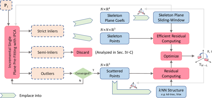
Figure 2: Overview of the plane pre-fitting and tracking pipeline. Shallow arrows $\rightarrow$ represent the operations to prepare for the next LiDAR scan.

IV Incremental Plane Pre-Fitting and Tracking

In this section, we first introduce our efficient plane pre-fitting method. Then, we describe the corresponding skeleton tracking algorithm based on PPF. Finally, a sandwich layer is proposed to robustify the algorithm in complex scenes.

IV-A Incremental iPCA Plane Pre-Fitting

The core of our method can be described from 3 aspects: Pre-Fitting, Iterative PCA and Incremental.

IV-A1 Pre-Fitting

The large surfaces across each scan form the basic skeleton of the 3D scene and reveal its global geometry feature. We refer to them as the skeleton planes, which are independently maintained instead of lazily fitted by kNN. We first take input from the extracted surface feature points [5] or the raw de-skewed cloud [4, 3]. Then, we adopt an iterative fit-remove-fit manner to extract all skeleton planes in $\mathbf{P}_{i}$. As for single plane fitting, we use the classic RANSAC [19] and NAPSAC [24]. The NAPSAC assumes that samples within the same class are closer to each other than points outside the class. Hence, samples from inside the same hyper-sphere are more likely to fit the best candidate model, but again, this requires the expensive kNN to guarantee. Thus, in most cases, simply increasing the RANSAC iterations can reach the same level of accuracy. Once a skeleton plane is fitted, all points are divided into strict inliers, semi-inliers (Sec. IV-C) and outliers according to their distance to the plane. All semi-inliers are directly discarded (analyzed later), and the outliers are fed into this process again. Since the skeleton tracking is effective for large planes, the loop terminates when no more qualified planes can be extracted or the remaining points are too few.

IV-A2 Iterative PCA Refining

Applying PCA to kNN dates back to [8], with the only purpose of determining whether more than 3 points can fit a plane. For the PPF, it can be more useful. Due to the noise of LiDAR sampling, IMU noise, bias and its random walk, de-skewed point clouds are noisy.

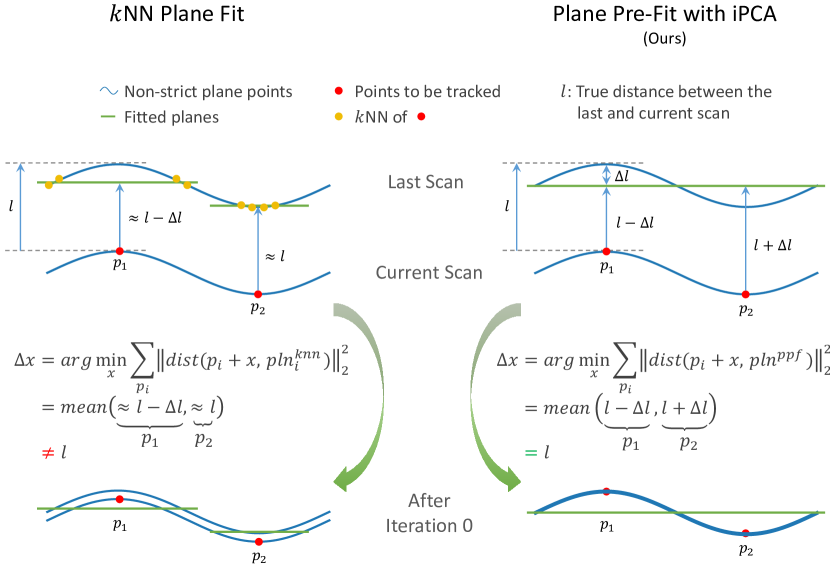
Figure 3: Illustration of the kNN degradation when tracking non-strict planes with small local curvature. The kNN strategy minimizes the point-to-local-plane distances. However, the local space determined by 4 NN cannot reflect the overall geometric forms. In contrast, the iPCA manner iteratively extracts the principal skeleton of all global planar points, resulting in faster convergence. Experimental validation in Sec. V-B.

Even in strict real-world planes (e.g. walls), non-negligible offsets between points and the corresponding plane still exist. On the other hand, some flat surfaces which are not strict planes can also have low local curvature (e.g. uneven grounds, small-angle arcs). Fig. 3 demonstrates the issue of kNN degradation in these cases. The kNN strategy uses only 4$\sim$5 NN, meaning that the fitted plane is determined by a small local space. When encountering large noise or non-strict planes, the local space cannot characterize the overall forms, thereby misleading the optimizing objective of the registration (see Fig. 3 left). On the contrary, the pre-fitting manner can make use of all planar points’ spatial information to produce their global skeleton plane. In particular, based on the current fitted plane, the eigen-decomposition is performed on the covariance matrix of all its strict inliers, and the resulting eigenvector associated with the smallest eigenvalue corresponds to the refined plane, which can be understood as newly voted by all the points that strictly support the old plane. The new strict inliers are computed accordingly and the process is looped 3 times [26]. We draw a conclusion in Fig. 3 that this iterative refinement brings PPF a faster convergence than kNN, which is further validated by more detailed comparative experiments in Sec. V-B.

IV-A3 Incremental Fitting

The geometry structures of adjacent LiDAR scans do not vary a lot, instead, they are generally similar. Inspired by this property, skeleton planes can be updated incrementally so that unnecessary RANSAC iterations will be saved. We first integrate (discrete-time, first-order hold) the IMU measurements between two consecutive LiDAR scans by iterating:

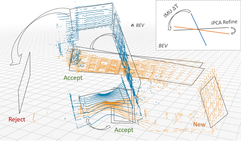
Figure 4: Illustration of the incremental fitting for the two scans in Fig. 1b (before scan-matching). Bird’s-Eye-View on top right. We discard the initial skeleton guesses that failed the inliers check. For those accepted, a simple iPCA refinement is performed. Only a few are newly fitted from RANSAC.

$$\bm{\omega}=\frac{1}{2}\left(\left(\hat{\bm{\omega}}_{k}-\mathbf{b}^{\bm{\omega}}_{k}\right)+\left(\hat{\bm{\omega}}_{k+1}-\mathbf{b}^{\bm{\omega}}_{k}\right)\right)$$ (3)

$$\mathbf{R}^{\mathbf{B}_{i}}_{\mathbf{B}_{k+1}}=\mathbf{R}^{\mathbf{B}_{i}}_{\mathbf{B}_{k}}\mathbf{exp}(\bm{\omega}\Delta t)$$ (4)

$$\mathbf{a}=\frac{1}{2}\left(\mathbf{R}^{\mathbf{B}_{i}}_{\mathbf{B}_{k}}\left(\hat{\mathbf{a}}_{k}-\mathbf{b}^{\mathbf{a}}_{k}\right)+\mathbf{R}^{\mathbf{B}_{i}}_{\mathbf{B}_{k+1}}\left(\hat{\mathbf{a}}_{k+1}-\mathbf{b}^{\mathbf{a}}_{k}\right)\right)$$ (5)

$$\mathbf{p}^{\mathbf{B}_{i}}_{\mathbf{B}_{k+1}}=\mathbf{p}^{\mathbf{B}_{i}}_{\mathbf{B}_{k}}+\mathbf{v}^{\mathbf{B}_{i}}_{\mathbf{B}_{k}}\Delta t+\frac{1}{2}\mathbf{a}\Delta t^{2}+\frac{1}{2}\mathbf{R}_{\mathbf{B}_{i}}^{\mathbf{W}\top}\mathbf{g}\Delta t^{2}$$ (6)

$$\mathbf{v}^{\mathbf{B}_{i}}_{\mathbf{B}_{k+1}}=\mathbf{v}^{\mathbf{B}_{i}}_{\mathbf{B}_{k}}+\mathbf{a}\Delta t+\mathbf{R}_{\mathbf{B}_{i}}^{\mathbf{W}\top}\mathbf{g}\Delta t,$$ (7)

where $k\in[i,j]$ is the IMU sampling instant between consecutive LiDAR sampling instants $i$ and $j$. $\Delta t$ is the IMU sampling interval. $\hat{\bm{\omega}}_{k}$ and $\hat{\bm{a}}_{k}$ are the raw IMU angular velocity and acceleration measurements at time $k$ in $\mathbf{B}$. IMU gyroscope bias $\mathbf{b}^{\bm{\omega}}$ and accelerator bias $\mathbf{b}^{\bm{a}}$ are modeled as random walk [27], whose derivatives are Gaussian white noise. $\mathbf{g}$ is the gravity vector in $\mathbf{W}$. Please refer to [28] for detailed derivations of Eqs. (3-7).

Next, for every incoming LiDAR scan $\mathbf{P}_{j}$, each current skeleton plane $\bm{f}_{\mathbf{L}_{i}}$ is used to obtain a corresponding initial skeleton guess $\bm{f}_{init}$ in $\mathbf{P}_{j}$ by:

$$\bm{f}_{init}=\bm{f}_{\mathbf{L}_{j}}=\left(\Delta\mathbf{T}^{-1}\right)^{\top}\bm{f}_{\mathbf{L}_{i}},~{}where$$ (8)

$$\Delta\mathbf{T}=\begin{bmatrix}\mathbf{R}^{\mathbf{L}}_{\mathbf{B}}\mathbf{R}^{\mathbf{B}_{i}}_{\mathbf{B}_{j}}\mathbf{R}^{\mathbf{L}\top}_{\mathbf{B}}&\mathbf{R}^{\mathbf{L}}_{\mathbf{B}}\mathbf{p}^{\mathbf{B}_{i}}_{\mathbf{B}_{j}}+\mathbf{t}^{\mathbf{L}}_{\mathbf{B}}-\mathbf{R}^{\mathbf{L}_{i}}_{\mathbf{L}_{j}}\mathbf{t}^{\mathbf{L}}_{\mathbf{B}}\\ \mathbf{0}_{1\times 3}&1\end{bmatrix},$$ (9)

$\mathbf{R}^{\mathbf{L}}_{\mathbf{B}}$ and $\mathbf{t}^{\mathbf{L}}_{\mathbf{B}}$ are the extrinsics between LiDAR and IMU. Note that the IMU-integrated $\Delta\mathbf{T}$ is not required to be very accurate, since it is only to provide a guess. $\bm{f}_{init}$ is accepted only if it passed the inliers checking. Once accepted, $\bm{f}_{init}$ will also be iPCA refined for 5 iterations. After handling the initial guesses, the naive RANSAC begins. We emphasize that this technique is particularly effective for LiDARs with high beam numbers, e.g., for Velodyne HDL-64E in KITTI dataset, the fitting algorithm can be boosted up to 4$\times$ faster.

IV-B Skeleton-based Tracking

Based on PPF, we describe the efficient residual evaluation criterion. During the iterative fitting, after refining every skeleton plane, we emplace its strict inliers into a set, denoted as $\mathbf{\Omega}$. When the PPF converges, the remaining points are considered to lie scatteredly. We denote the set containing the scattered points as $\mathbf{\Theta}$. Note that the semi-inliers are discarded so we have $\mathbf{\Omega}\cup\mathbf{\Theta}\subseteq\mathbf{P}$. For each skeleton point $\tilde{\mathbf{p}}$ in $\mathbf{\Omega}$, we search its correspondence in the skeleton plane space $\mathbf{F}$. $\mathbf{F}$ is implemented as a sliding window of $\bm{f}$ in $\mathbf{W}$. The residual is measured as point-to-nearest-plane distance:

$$e_{\Omega}\left(\tilde{\mathbf{p}}\right)=\begin{cases}0,~{}~{}~{}\min_{\bm{f}\in\mathbf{F}}\left\{\lvert\,\bm{f}\cdot\tilde{\mathbf{p}}\,\rvert\right\}\geq\epsilon\\ \min_{\bm{f}\in\mathbf{F}}\left\{\lvert\,\bm{f}\cdot\tilde{\mathbf{p}}\,\rvert\right\},~{}~{}~{}otherwise.\end{cases}$$ (10)

While for $\tilde{\mathbf{p}}$ in $\mathbf{\Theta}$, the searching still happens at point level, i.e. building the e.g. kd-tree or iVox for the local map to search k NN points, and the residual is based on the distance between $\tilde{\mathbf{p}}$ and the lazily fitted plane patch $\bm{f}_{knn}$ [3, 5]:

$$e_{\Theta}\left(\tilde{\mathbf{p}}\right)=\lvert\,\bm{f}_{knn}\cdot\tilde{\mathbf{p}}\,\rvert.$$ (11)

Next, the scan-matching algorithm registers the latest LiDAR scan by solving for the optimal transformation

$$\min_{\mathbf{T}_{j}}\Big{\{}\sum_{\tilde{\mathbf{p}}\in\mathbf{\Omega}}e_{\Omega}\left(\tilde{\mathbf{p}}\right)+\sum_{\tilde{\mathbf{p}}\in\mathbf{\Theta}}e_{\Theta}\left(\tilde{\mathbf{p}}\right)\Big{\}},$$ (12)

using Levenberg-Marquardt [29, 5] or IEKF [3]. Then, in preparation for the next LiDAR scan, we transform all the newly-fitted $\bm{f}_{\mathbf{L}_{j}}$ to $\mathbf{W}$, i.e. $\bm{f}_{\mathbf{W}}=\left(\mathbf{T}_{j}^{-1}\right)^{\top}\bm{f}_{\mathbf{L}_{j}}$, and emplace $\bm{f}_{\mathbf{W}}$ into the sliding window $\mathbf{F}$. Note that although points in $\mathbf{\Omega}$ outnumber $\mathbf{\Theta}$, the searching space of $\mathbf{\Omega}$ (i.e. $\mathbf{F}$) is about three orders of magnitude smaller than that of $\mathbf{\Theta}$.

IV-C Sandwich Layer

When entering new scenes, there could be no plane match in $\mathbf{F}$ for points on the newly fitted skeleton planes. Rather, since planes intersect, there may exist false matches if solely relying on point-to-plane distance. This is more severe for planes with small included angles.

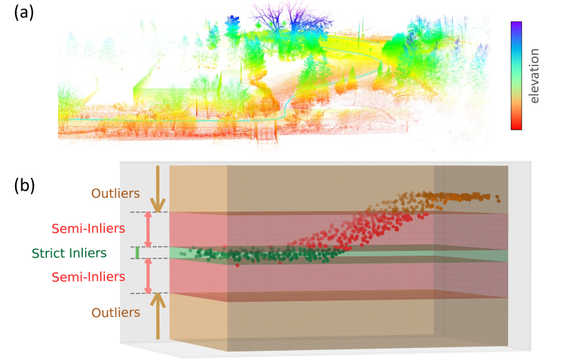
Figure 5: (a) A scene with grounds of different elevations. (b) Schematic of the slope ground in (a) and the sandwich layer used in PPF. According to the distance to the central plane, points are categorized into three groups: strict inliers, semi-inliers and outliers.

E.g., the complex terrain in Fig. 5a, where the ground elevation slowly rises due to the slope. Assuming this is the first scan fitting the slope plane such that it is not emplaced into $\mathbf{F}$ yet, points on the slope can easily pass the check in (10) and hence wrongly match the ground plane. To handle this, we introduce an additional semi-inlier layer (Fig. 5b). Before the scan-matching, we simply discard all semi-inlier points, which may lead to potentially false matches. The thickness of the semi-inlier layer is set to be $\epsilon$ so that outliers can hardly produce false matches. On the other hand, this also helps prevent the noisy ‘thick’ planar points from yielding multi skeleton planes - we only use points strictly s.t. the central plane as skeleton. The removal is so straightforward because the proportion of these ambiguous points is small and their negative impact far outweighs their contributions to the tracking.

V Experiments

V-A Datasets and Experiment Setup

All experiments were conducted using a modern desktop computer with Ubuntu 18.04 LTS. We use a single Intel Core i7-9700K (3.60G Hz × 8 cores) CPU with 16 GiB memory without using GPU. The OpenMP [25] library is adopted for parallel computing. For the sake of fair comparisons with previous methods, in all experiments, we launched the same number of threads in parallel as the one to be compared.

We first conducted comparative experiments to analyse the PPF registration strategy and the kNN-based one. Then, we extensively evaluate the accuracy and efficiency of our PPF-based LIO in real-world scenarios. We test on 5 public datasets, i.e. UTBM robocar dataset [30], KITTI [31], LIOSAM [5], ULHK [32] and NCLT [33], including 22 sequences in total. See Appendix for benchmark details.

V-B Comparative Study of PPF and kNN

In this section, we verify the conclusion drawn in Fig. 3: The PPF takes fewer iterations to converge than kNN, and costs at least an order of magnitude less time in every single iteration.

We generate planes with Gaussian white noise, which, in the real world, may come from LiDAR sampling, cloud de-skewing with noisy IMU measurements, etc. To simulate the agent’s ego-motion, a distance is set between the two planes. The goal is to register these two scans such that different scans of the same object can overlap in the mapping.

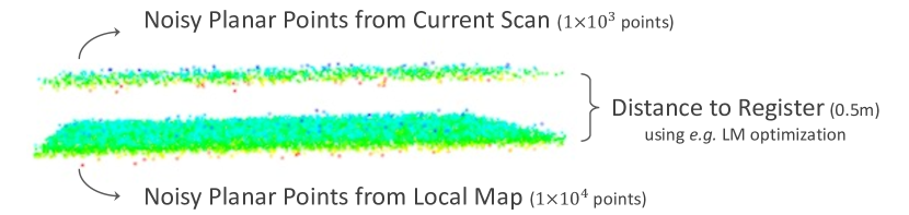
Figure 6: Simulated experiment setup. We generate planes with Gaussian white noise of varying $stddev$. The registration is done with different point matching strategies using the Levenberg-Marquardt algorithm [29].

Results are shown in Fig. 7. We first plot the distance between two planes w.r.t. the number of iterations in (a). For the PPF strategy, regardless of the Gaussian noise $stddev$, the registrations are almost done only after the first iteration (i.e. distance $\approx$ $0\mathrm{m}$, overlap). While for the kNN strategy, as the noise grows, the registrations of the first few iterations perform poorly. This is because with the increase of noise $std$, the 4$\sim$5 NN become unstable and hence the fitted plane gradually deviates from the central plane, thereby misleading the optimizing objective. Note that applying PCA refinement on kNN-fitted planes can hardly reduce the negative effects of noise, because the samples for fitting (k) are too few, resulting in the principal component being sensitive to any slight deviations caused by the noise. Next, we show the number of iterations to converge w.r.t. the noise $std$ in (b).

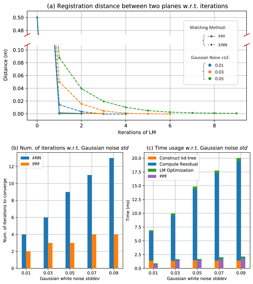
Figure 7: Results of the simulation experiments. (c) left bar: kNN; right bar: PPF. All experiments run in a single thread.

Generally, PPF is more robust to noise, and the number of iterations needed increases at a much lower rate. We further compare the detailed runtime of the two strategies in (c). The overall efficiency of PPF is significantly higher. The kNN strategy spends most of the time in residual computation, which includes the expensive kNN search and plane fitting for each point. Again, these operations are redundant and can be saved if searching happens at the plane level. As a result, the residual computing time of PPF is at least one order of magnitude less than that in kNN. From the trend of the overall runtime w.r.t. noise, kNN grows at a much faster speed, whereas the PPF keeps at a stable level. The time growth of kNN stems mainly from the number of iterations, and the growth of PPF comes only from pre-fitting. This is because the iPCA refinement takes more time to converge when the noise is large. However, once the skeleton plane is determined, the LM optimization and residual calculation are no longer affected by the noise of point clouds.

TABLE I: Time ($\mathrm{ms}$) and Memory Consuming of Each Step in LIO-SAM [5] Using kNN or PPF

Dataset	PPF		Build Local Map		Build kd-tree		Scan Match		Calc. Residual		Total time1		Local Map Size2
	kNN	PPF	kNN	PPF	kNN	PPF	kNN	PPF	kNN	PPF	kNN	PPF	kNN	PPF
LIOSAM-3	0	2.64	21.28	10.48	8.43	5.51	19.97	13.84	1.50	0.69	45.12	30.80	66.9k	44.1k
LIOSAM-4	0	3.16	28.12	13.65	9.56	6.25	21.99	15.96	1.66	0.76	54.36	36.98	75.8k	49.9k
LIOSAM-5	0	3.07	18.20	9.97	8.55	6.05	22.03	17.51	2.01	0.97	44.37	34.69	67.9k	48.3k
LIOSAM-2	0	3.61	17.69	10.33	8.88	6.36	23.36	18.55	2.11	1.14	44.95	36.39	70.4k	50.5k
KITTI-7	0	1.30†	55.08	21.56	8.20	3.72	42.93	19.47	3.95	0.83	112.66	58.73	67.6k	29.4k
KITTI-2	0	1.96†	36.76	13.95	5.19	2.61	35.63	16.99	3.80	0.99	91.25	51.77	41.6k	15.7k
KITTI-3	0	1.50†	44.55	24.30	4.30	2.75	28.96	17.48	2.49	0.78	93.05	62.82	37.0k	19.5k
KITTI-4	0	1.25†	45.86	21.92	4.37	2.32	28.47	15.23	2.95	0.73	93.96	58.02	37.3k	17.0k
KITTI-6	0	1.48†	43.29	17.32	5.48	2.34	30.96	15.15	4.12	0.90	93.23	52.93	44.3k	15.9k
KITTI-5	0	1.22†	55.24	23.11	7.31	3.44	43.17	21.10	3.52	0.73	114.89	64.43	60.8k	26.6k
KITTI-1	0	1.29†	45.04	22.79	4.70	2.69	32.25	17.98	3.07	0.80	97.18	61.96	40.3k	19.8k

• The total time includes some common steps e.g. de-skewing (not listed) whose timings are unchanged - we only tabulate steps which are sped up.

• The local map denotes the one used in the scan-matching algorithm, not the reconstructed map. We only decrease the memory usage of LIO algorithms but do not decrease the quality of the mapping. The size is measured by the number of points.

• The incremental fitting is enabled for KITTI dataset, to show the benefits for handling the large number of points obtained by Velodyne HDL-64E Laser scanner.

TABLE II: Accuracy Comparison of LIO-SAM [5] Using kNN and PPF

Dataset	LIO-SAM		LIO-SAM w/ PPF
	APE $(\mathrm{m})$	RPE $(\mathrm{m})$	APE $(\mathrm{m})$	RPE $(\mathrm{m})$
LIOSAM-1	0.739	6.928	0.719	6.742
LIOSAM-2	9.785	14.387	8.364	13.353
LIOSAM-5	1.365	2.620	1.280	2.624
KITTI-1†	2.039	0.105	2.026	0.101
KITTI-2†	1.551	1.336	1.547	1.335
KITTI-3†	1.209	0.344	1.398	0.332
KITTI-4†	1.268	0.152	0.960	0.162
KITTI-6†	0.342	0.055	0.328	0.048
KITTI-7†∗	4.463	1.471	3.147	1.461

• Since LIO-SAM requires high-frequency IMU, the Rosbag of KITTI Odom is generated from the corresponding KITTI Raw data.

Figure 8: Mapping results of the MIT campus using LIOSAM-3 sequence.

V-C Efficiency Evaluation

LIO systems’ efficiencies are evaluated by analyzing the runtime of each step. In order to investigate how LIO systems can benefit from the PPF, we first redevelop LIO-SAM [5] and compare the efficiency using kNN and PPF. We tabulate the detailed time cost of each step in Tab. I. In the LIOSAM datasets, the overall efficiency (FPS, $\frac{1}{total\>time}$) is increased to 140% $\sim$ 150%. In the park sequence, the basic skeleton is not clear due to the large amount of vegetation (tree leaves, grass), hence the FPS is only increased to 128%. Specifically, since skeleton points are all extracted out and tracked independently, the efficiencies of local map construction and kd-tree building are greatly boosted, with only an extra cost of $3\,\mathrm{ms}$ from pre-fitting. In terms of the searching space, the basic skeleton is stored in a sliding window $\mathbf{F}$ with at most 5 plane coef $\in\mathbb{R}^{4}$, which is much smaller than the local point map, and the expensive kNN search is totally abandoned here. Consequently, time to calculate residuals is reduced by more than half. To better show the benefit of PPF, we disable the point cloud down-sampling in KITTI dataset, and make use of all points available. This also helps LIO to reconstruct more fine-grained 3D maps. The overall FPS is increased more significantly in KITTI, which is up to 1.92$\times$. Note that there are even two sequences that cannot run in real time without PPF. The residual calculation’s efficiency can also be increased to more than 4$\times$ faster. The local map memory usage is reduced to a minimum of 36%. Meanwhile, because of the heavy Velodyne HDL-64E Laser scanner of KITTI, we enable the incremental fitting, which further decreases the time of PPF from $\sim 6\,\mathrm{ms}$ (not tabulated) to $\sim 1.5\,\mathrm{ms}$.

Figure 9: Estimated trajectory and reconstructed maps of a large-scale scene in the University of Michigan North Campus, aligned with Google Earth.

V-D Accuracy Evaluation

The accuracy is measured by root mean square error (RMSE) of absolute pose error (APE) metric and relative pose error (RPE) metric, which were calculated by evo [34] in our experiments. We first compare the accuracy of our algorithm with LIO-SAM, as reported in Tab. II. In LIOSAM dataset, 3 sequences are with GPS measurements, which are treated as ground truth trajectories. Since LIO-SAM requires high-frequency IMU measurements, all KITTI sequences are generated from KITTI-RAW dataset using $kitti\_to\_bag$ toolkit. We also show the accuracy results of integrating PPF into other state-of-the-art LIO systems, e.g. Faster-LIO [4]. The accuracies of 4 systems are compared in 9 sequences in Tab. III. Since LIO-SAM requires a 9-axis IMU, which is not available in the UTBM dataset, the results are not shown. Some sequences provide the ground truth poses at a low frequency (e.g. 1 hz in ULHK), therefore, we adjust the t_max_diff parameter of evo to increase the maximum timestamp difference for data association. As can be seen, with kNN replaced by PPF, both LIO-SAM and Faster-LIO can reach a generally comparable accuracy to their original counterparts, with less time and memory usage. Visualizations of estimated trajectories are compared in Fig. 10, which also shows that the ones with PPF keep the same level of accuracy in most sequences (sometimes even more visually accurate, e.g. the KITTI-7 sequence).

TABLE III: Accuracy Comparison of Existing State-of-the-Art Methods

Dataset	Faster-LIO [4]		Faster-LIO w/ PPF		LIO-SAM [5]		LiLi-OM [6]		Distance (km)
	APE $(\mathrm{m})$	RPE $(\%)$	APE $(\mathrm{m})$	RPE $(\%)$	APE $(\mathrm{m})$	RPE $(\%)$	APE $(\mathrm{m})$	RPE $(\%)$
NCLT-1	1.239	0.157	1.365	0.157	10.095	1.307	-	-	1.14
NCLT-2	1.478	0.153	1.230	0.153	26.351	1.309	-	-	3.19
UTBM-1	26.519	1.806	27.470	1.800	-	-	14.950	5.669	6.40
UTBM-6	15.989	0.876	16.857	0.866	-	-	12.954	4.124	5.14
UTBM-3	15.510	0.482	16.502	0.474	-	-	15.989	2.869	4.98
UTBM-2	15.002	1.983	14.996	1.985	-	-	24.466	12.051	4.99
UTBM-4	14.560	2.036	15.701	2.034	-	-	13.654	12.735	4.99
ULHK-1	0.972	0.915	1.038	0.631	1.503	0.931	0.964	0.635	0.60
ULHK-2	0.888	0.443	0.897	0.421	0.926	0.465	0.893	0.417	0.62

TABLE IV: Runtime ($\mathrm{ms}$) Comparison of Fast-LIO2 [3] Using kNN and PPF

Dataset	Calc. Residual	Map Incremental	IEKF	Map Size1
NCLT-2	2.79	1.52	12.67	3.37k
w/ PPF	1.90	1.26	8.73	2.33k
NCLT-1	2.54	1.56	11.66	2.74k
w/ PPF	1.72	1.28	7.98	1.89k
UTBM-5	2.90	3.66	13.86	3.29k
w/ PPF	1.57	2.62	7.95	1.81k
UTBM-2	2.88	3.34	13.49	3.34k
w/ PPF	1.83	2.64	9.06	2.14k
UTBM-4	2.68	3.16	12.64	3.30k
w/ PPF	1.81	2.58	8.87	2.14k
UTBM-3	2.74	3.39	12.97	3.29k
w/ PPF	1.76	2.61	8.71	2.08k
UTBM-6	2.80	3.27	13.33	3.31k
w/ PPF	1.70	2.45	8.57	2.07k
ULHK-1	2.87	2.08	13.64	2.79k
w/ PPF	1.37	1.47	7.39	1.27k
ULHK-2	2.96	2.01	14.03	2.83k
w/ PPF	1.44	1.45	7.65	1.30k

• Map memory is measured by the average number of new points in each scan that need to be maintained by the ikd-tree.

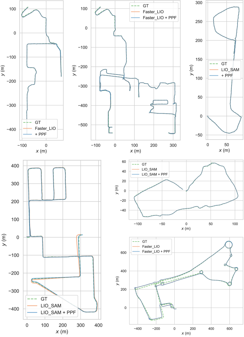
Figure 10: The estimated and GT trajctories. From top left to bottom right: NCLT-1, NCLT-2, LIOSAM-5, KITTI-7, LIOSAM-1 and UTBM-5.

VI Conclusion

We investigate the computation of LiDAR-Inertial odometry systems, and reveal the redundancy of most kNN searches, plane fittings and the un-necessity of the large local map. To achieve more efficient LiDAR scan tracking, we design a plane pre-fitting pipeline to achieve the basic-skeleton tracking. We demonstrate the un-robustness of kNN to noisy and non-strict planes, and introduce iPCA to PPF to handle this. Moreover, skeleton planes can be incrementally updated by leveraging IMU measurements and the sequential nature of LiDAR scans to further speed up PPF. For complex scenarios where planes can have small included angles, a simple yet effective sandwich layer is introduced to eliminate false point-to-plane matches. Experiments on 22 sequences across 5 open datasets show that, by contrast, our skeleton tracking consumes only a minimum of 36% of the original local map size, achieving 4$\times$ faster in residual computing and up to 1.92$\times$ overall FPS, while maintaining the same level of accuracy. To make contributions to the SLAM community, we publish the full C++ implementation of this paper.

APPENDIX

TABLE V: Details of All the 22 Sequences Used in Sec. V

	Sequence	Duration $(\mathrm{min:sec})$	Distance $(\mathrm{km})$
LIOSAM-1	Campus (small)	6:47	0.55
LIOSAM-2	Campus (large)	16:34	1.44
LIOSAM-3	Walking	10:55	0.80
LIOSAM-4	Garden	6:02	0.46
LIOSAM-5	Park	9:20	0.65
NCLT-1	2013_01_10	17:05	1.14
NCLT-2	2012_04_29	43:19	3.19
UTBM-1	2019_01_31	16:00	6.40
UTBM-2	2018_07_17	15:59	4.99
UTBM-3	2018_07_19	15:26	4.98
UTBM-4	2018_07_20	16:45	4.99
UTBM-5	2019_04_12 roundabout	12:10	4.86
UTBM-6	2019_04_18	14:55	5.14
ULHK-1	2019_01_17	5:18	0.60
ULHK-2	2019_03_17	5:18	0.62
KITTI-1	Raw 2011_09_30_drive_0034	2:07	0.92
KITTI-2	Raw 2011_09_26_drive_0002	0:08	0.08
KITTI-3	Raw 2011_09_26_drive_0061	1:12	0.49
KITTI-4	Raw 2011_09_26_drive_0064	0:59	0.44
KITTI-5	Raw 2011_09_30_drive_0018	4:48	2.21
KITTI-6	Raw 2011_09_26_drive_0084	0:40	0.24
KITTI-7	Odometry Seq. 08	8:56	3.22

References

- [1] J. Zhang and S. Singh, “LOAM: Lidar odometry and mapping in real-time.” in Robotics: Science and Systems, vol. 2, no. 9. Berkeley, CA, 2014, pp. 1–9.
- [2] W. Xu and F. Zhang, “Fast-LIO: A fast, robust lidar-inertial odometry package by tightly-coupled iterated kalman filter,” IEEE Robotics and Automation Letters, vol. 6, no. 2, pp. 3317–3324, 2021.
- [3] W. Xu, Y. Cai, D. He, J. Lin, and F. Zhang, “Fast-LIO2: Fast direct lidar-inertial odometry,” IEEE Transactions on Robotics, 2022.
- [4] C. Bai, T. Xiao, Y. Chen, H. Wang, F. Zhang, and X. Gao, “Faster-lio: Lightweight tightly coupled lidar-inertial odometry using parallel sparse incremental voxels,” IEEE Robotics and Automation Letters, vol. 7, no. 2, pp. 4861–4868, 2022.
- [5] T. Shan, B. Englot, D. Meyers, W. Wang, C. Ratti, and D. Rus, “Lio-sam: Tightly-coupled lidar inertial odometry via smoothing and mapping,” in 2020 IEEE/RSJ international conference on intelligent robots and systems (IROS). IEEE, 2020, pp. 5135–5142.
- [6] K. Li, M. Li, and U. D. Hanebeck, “Towards high-performance solid-state-lidar-inertial odometry and mapping,” IEEE Robotics and Automation Letters, vol. 6, no. 3, pp. 5167–5174, 2021.
- [7] C. Qin, H. Ye, C. E. Pranata, J. Han, S. Zhang, and M. Liu, “LINS: A lidar-inertial state estimator for robust and efficient navigation,” in 2020 IEEE international conference on robotics and automation (ICRA). IEEE, 2020, pp. 8899–8906.
- [8] J. Zhang and S. Singh, “Low-drift and real-time lidar odometry and mapping,” Autonomous Robots, vol. 41, no. 2, pp. 401–416, 2017.
- [9] T. Shan and B. Englot, “LeGO-LOAM: Lightweight and ground-optimized lidar odometry and mapping on variable terrain,” in 2018 IEEE/RSJ International Conference on Intelligent Robots and Systems (IROS). IEEE, 2018, pp. 4758–4765.
- [10] H. Ye, Y. Chen, and M. Liu, “Tightly coupled 3d lidar inertial odometry and mapping,” in 2019 International Conference on Robotics and Automation (ICRA). IEEE, 2019, pp. 3144–3150.
- [11] L. Zhou, D. Koppel, and M. Kaess, “Lidar slam with plane adjustment for indoor environment,” IEEE Robotics and Automation Letters, vol. 6, no. 4, pp. 7073–7080, 2021.
- [12] L. Zhou, G. Huang, Y. Mao, J. Yu, S. Wang, and M. Kaess, “-lislam: Lidar slam with planes, lines, and cylinders,” IEEE Robotics and Automation Letters, vol. 7, no. 3, pp. 7163–7170, 2022.
- [13] Y. Cai, W. Xu, and F. Zhang, “ikd-Tree: An incremental kd tree for robotic applications,” arXiv preprint arXiv:2102.10808, 2021.
- [14] R. Farid, “Region-growing planar segmentation for robot action planning,” in AI 2015: Advances in Artificial Intelligence: 28th Australasian Joint Conference, Canberra, ACT, Australia, November 30–December 4, 2015, Proceedings 28. Springer, 2015, pp. 179–191.
- [15] H. Wu, X. Zhang, W. Shi, S. Song, A. Cardenas-Tristan, and K. Li, “An accurate and robust region-growing algorithm for plane segmentation of tls point clouds using a multiscale tensor voting method,” IEEE Journal of Selected Topics in Applied Earth Observations and Remote Sensing, vol. 12, no. 10, pp. 4160–4168, 2019.
- [16] R. Hulik, M. Spanel, P. Smrz, and Z. Materna, “Continuous plane detection in point-cloud data based on 3d hough transform,” Journal of visual communication and image representation, vol. 25, no. 1, pp. 86–97, 2014.
- [17] X. Leng, J. Xiao, and Y. Wang, “A multi-scale plane-detection method based on the hough transform and region growing,” The Photogrammetric Record, vol. 31, no. 154, pp. 166–192, 2016.
- [18] B. Oehler, J. Stueckler, J. Welle, D. Schulz, and S. Behnke, “Efficient multi-resolution plane segmentation of 3d point clouds,” in Intelligent Robotics and Applications: 4th International Conference, ICIRA 2011, Aachen, Germany, December 6-8, 2011, Proceedings, Part II 4. Springer, 2011, pp. 145–156.
- [19] M. A. Fischler and R. C. Bolles, “Random sample consensus: a paradigm for model fitting with applications to image analysis and automated cartography,” Communications of the ACM, vol. 24, no. 6, pp. 381–395, 1981.
- [20] A. Khaloo and D. Lattanzi, “Robust normal estimation and region growing segmentation of infrastructure 3d point cloud models,” Advanced Engineering Informatics, vol. 34, pp. 1–16, 2017.
- [21] W. Yue, J. Lu, W. Zhou, and Y. Miao, “A new plane segmentation method of point cloud based on mean shift and ransac,” in 2018 Chinese Control And Decision Conference (CCDC). IEEE, 2018, pp. 1658–1663.
- [22] L. Li, F. Yang, H. Zhu, D. Li, Y. Li, and L. Tang, “An improved ransac for 3d point cloud plane segmentation based on normal distribution transformation cells,” Remote Sensing, vol. 9, no. 5, p. 433, 2017.
- [23] D. Xu, F. Li, and H. Wei, “3d point cloud plane segmentation method based on ransac and support vector machine,” in 2019 14th IEEE Conference on Industrial Electronics and Applications (ICIEA). IEEE, 2019, pp. 943–948.
- [24] P. H. Torr, S. J. Nasuto, and J. M. Bishop, “NAPSAC: High noise, high dimensional robust estimation-it’s in the bag,” in British Machine Vision Conference (BMVC), vol. 2, 2002, p. 3.
- [25] L. Dagum and R. Menon, “OpenMP: an industry standard api for shared-memory programming,” IEEE computational science and engineering, vol. 5, no. 1, pp. 46–55, 1998.
- [26] R. B. Rusu and S. Cousins, “3D is here: Point Cloud Library (PCL),” in IEEE International Conference on Robotics and Automation (ICRA). Shanghai, China: IEEE, May 9-13 2011.
- [27] T. Qin, P. Li, and S. Shen, “Vins-mono: A robust and versatile monocular visual-inertial state estimator,” IEEE Transactions on Robotics, vol. 34, no. 4, pp. 1004–1020, 2018.
- [28] C. Forster, L. Carlone, F. Dellaert, and D. Scaramuzza, “On-manifold preintegration for real-time visual–inertial odometry,” IEEE Transactions on Robotics, vol. 33, no. 1, pp. 1–21, 2016.
- [29] J. J. Moré, “The levenberg-marquardt algorithm: implementation and theory,” in Numerical analysis. Springer, 1978, pp. 105–116.
- [30] Z. Yan, L. Sun, T. Krajnik, and Y. Ruichek, “EU long-term dataset with multiple sensors for autonomous driving,” in Proceedings of the 2020 IEEE/RSJ International Conference on Intelligent Robots and Systems (IROS), 2020.
- [31] A. Geiger, P. Lenz, and R. Urtasun, “Are we ready for autonomous driving? the kitti vision benchmark suite,” in 2012 IEEE conference on computer vision and pattern recognition. IEEE, 2012, pp. 3354–3361.
- [32] W. Wen, Y. Zhou, G. Zhang, S. Fahandezh-Saadi, X. Bai, W. Zhan, M. Tomizuka, and L.-T. Hsu, “Urbanloco: A full sensor suite dataset for mapping and localization in urban scenes,” in 2020 IEEE International Conference on Robotics and Automation (ICRA). IEEE, 2020, pp. 2310–2316.
- [33] N. Carlevaris-Bianco, A. K. Ushani, and R. M. Eustice, “University of Michigan North Campus long-term vision and lidar dataset,” International Journal of Robotics Research, vol. 35, no. 9, pp. 1023–1035, 2015.
- [34] M. Grupp, “evo: Python package for the evaluation of odometry and slam.” https://github.com/MichaelGrupp/evo, 2017.