Formation of Exceptional Points in pseudo-Hermitian Systems
Abstract
Motivated by the recent growing interest in the field of -symmetric Hamiltonian systems we theoretically study the emergency of singularities called Exceptional Points (EPs) in the eigenspectrum of pseudo-Hermitian Hamiltonian as the strength of Hermiticity-breaking terms turns on. Using general symmetry arguments, we characterize the separate energy levels by a topological index which corresponds to the signs of the eigenvalues of pseudo-metric operator in the absence of Hermiticity-breaking terms. After that, we show explicitly that the formation of second-order EPs is governed by this -index: only the pairs of levels with opposite index can provide second-order EPs. Our general analysis is accompanied by a detailed study of EPs appearance in an exemplary -symmetric pseudo-Hermitian system with parity operator in the role of : a transverse-field Ising spin chain with a staggered imaginary longitudinal field. Using analytically computed parity indices of all the levels, we analyze the eigenspectrum of the model in general, and the formation of third-order EPs in particular.
I Introduction
Quantum mechanics on a macroscopic scale fascinates scientists for many years, and recently it becomes a firm basis of various applications in the field of Quantum Information, i.e., quantum computing, quantum simulators etc. [1]. However, the quantum mechanics applies to the isolated systems only, and for macroscopic systems interacting with an environment unavoidably present dissipation and decoherence lead to the degradation of coherent quantum properties, e.g., the decay of quantum beats or microwave induced Rabi oscillations with the time [1, 2].
A one natural way to describe the dynamics of dissipative quantum systems is to use non-Hermitian Hamiltonians. Indeed, a non-Hermitian Hamiltonian has complex eigenvalues, and e.g., an exponential decay of quantum properties that is typical for the dissipative quantum dynamics, can be easily obtained with this approach.
Beyond that the non-Hermitian systems have their own unique properties. Thus, one of the main drivers of the active research of non-Hermitian systems is the emergency of the singularity points in the eigenspectrum of a non-Hermitian Hamiltonian. Such points are called ”Exceptional Points” (EPs), and they correspond to the points in the parameter space of a non-Hermitian Hamiltonian, where two or more eigenvalues and corresponding eigenvectors coalesce, rendering the Hamiltonian non-diagonalizable [3, 4]. Second-order EPs have peculiar topological properties [5, 6], and can be used in various applications such as quantum sensors [7, 8, 9, 10], adiabatic time asymmetric quantum-state-exchange [11, 12], mode switching in waveguides [13, 14, 15, 16] and optical microcavities [17, 18, 19], laser emission management [20, 21] just to name a few.
Moreover, higher-order EPs, which involve three or more coalescing states, have been also theoretically studied, and there has already been a number of interesting proposals that utilize the higher-order EPs, e.g., an increase of the sensitivity of the quantum sensors [22], states conversion [23, 24] and speeding up entanglement generation [25].
A main challenge in realization of the quantum devices based on EPs is the need to tune a device to the vicinity of a given EP. The crucial step towards solution of this problem is to obtain general conditions determining the formation of EPs in non-Hermitian systems. Classification of EPs and quantification of the number of independent parameters required for fine-tuning of a system to the EP have been done in Refs. [26, 27, 28, 29]. The analysis carried out in these works was limited to the vicinities of EPs and focused on the states that coalesce at corresponding EPs. As such, this analysis provides only a partial picture as it does not allow to identify the specific states in the eigenspectrum of the Hamiltonian forming EPs as the Hermiticity-breaking terms are turned on.
The number of the parameters required for fine-tuning is reduced if the Hamiltonian is subject to a symmetry from the class of anti-unitary symmetries [26, 27, 28, 29]. This class includes parity–time-reversal (), parity–particle-hole (), pseudo-chiral and pseudo-Hermitian (psH) symmetries. These symmetries are not unrelated, as they all can be connected to the notion of pseudo-Hermiticity: The substitution turns -symmetry into -symmetry, while pseudo-chiral symmetry — into pseudo-Hermitian one [26]. Finally, -symmetric Hamiltonians are known to be pseudo-Hermitian [30, 31, 32, 33, 34, 35].
A pseudo-Hermitian Hamiltonian satisfies the following condition:
| (1) |
where is an invertible Hermitian operator, called a pseudo-metric operator. This condition leads to a special symmetry of the eigenspectrum of a pseudo-Hermitian Hamiltonian: the spectrum consists of purely real eigenvalues and pairs of complex conjugated eigenvalues, and the EPs separate the regions of parameters where the levels have real and complex eigenvalues.
In this paper, we are going to consider pseudo-Hermitian Hamiltonians, for which a globally invariant pseudo-metric can be chosen, that does not depend on the parameters of the Hamiltonian. This case corresponds to the pseudo-Hermitian (psH) symmetry of the Hamiltonian [28]. In comparison, for a -symmetric Hamiltonian, is not uniquely defined [36, 37], and it is not apriori known whether such globally invariant choice of can be made. Nevertheless, there are plenty of examples of -symmetric systems which are simultaneously psH-symmetric.
In the manuscript, we present a theoretical study of the formation of EPs in the eigenspectrum of an arbitrary psH-symmetric Hamiltonian under the assumption that there are no additional symmetries that would lead to symmetry protected degeneracies. We relate the formation of EPs to the topological -index corresponding to the signs of the eigenvalues of the pseudo-metric operator in the absence of Hermiticity-breaking terms.
Our general analysis is then applied to an exemplary model of transverse-field Ising spin chain in an imaginary staggered longitudinal magnetic field, which has been introduced by us in Ref. [38] in the context of the ground state quantum phase transitions. This model is psH-symmetric, and the parity operator can be chosen as the globally invariant pseudo-metric: . Interestingly enough, this model is simultaneously -symmetric. Since the parity is self-inverse operator with eigenvalues, the topological -index coincides in this case with the parity of a state at vanishing imaginary field. In the presence of the non-Hermitian terms, the model becomes non-integrable, however, if one turns these terms off, the model is exactly diagonalizable via the combination of the Jordan-Wigner and the generalized Bogolyubov transformations [39]. Using the analytically computed parities of all the states, we analyze the formation of EPs of second and third order in different regimes.
Such a model can be experimentally realized as an array of interacting -symmetric qubits (two-level systems), where imaginary longitudinal magnetic field corresponds to a proper combination of gain (loss). The quantum dynamics of -symmetric single qubit have been observed in numerous atomic or solid state systems such as trapped ions, ultracold and Rydberg atoms [40, 41, 42], Bose-Einstein condensate [43], superconducting [44, 45] or nitrogen-vacancies [46] qubits interacting with auxiliary qubits. In all these systems a non-equilibrium growth of the population of specially chosen quantum states, i.e., states with a gain, can be completely compensated by a loss present in the other states, and therefore, the -symmetric combination of gain and loss occurs. Moreover, recently the entanglement generation has been studied [25], and a general analysis have been used to identify different quantum regimes for two -symmetric interacting qubits [47].
The paper is organized as follows: In Section II, we define the topological -index and show that the eigenstates of a psH-symmetric Hamiltonian can be characterized by such -index in the regions of parameters where the corresponding eigenvalues stay real. In Section III, we derive the selection rules determining the formation of EPs in the eigenvalues spectrum of an arbitrary -symmetric Hamiltonian. In Section IV, we apply our general analysis elaborated in Sec. II and III to an exemplary psH-symmetric non-Hermitian system: transverse field Ising chain with staggered longitudinal gain and loss, and show how the formation of second-order and third-order EPs relates to the -indices of eigenstates, which are equivalent to the parities in this case. In Section V, we present the discussion of the results and conclusions.
II Definition of the -index of a state.
Let us consider a psH-symmetric Hamiltonian which depends on the vector of physical parameters :
| (2) |
Varying the parameters one can move the eigenvalues and eigenvectors of closer or further to the Exception points (EPs).
Away from EPs, one can introduce the complete bi-orthonormal set of left and right eigenvectors of the Hamiltonian [48]:
| (3) | ||||
| (4) |
| (5) |
Let us consider the right and the left eigenvectors of some state . For real values of we obtain by Hermitian conjugation of Eq. (4)
| (6) |
On the other hand, it follows from Eq. (2) that
| (7) |
Assuming that the state is not degenerate, we obtain
| (8) |
where is a real-valued coefficient. Indeed, it follows from the fact that
| (9) |
is the quantum average of Hermitian operator. Notice here that the bi-orthonormal set of the left and the right eigenvectors is defined up to the arbitrary rescaling factor providing that the equation (5) is satisfied. It means that one can multiply by some arbitrary complex function and simultaneously divide by this . After this rescaling, the relation between and becomes
| (10) |
Choosing we obtain
| (11) |
where
| (12) |
is the -index of the state .
As we see from Eq. (12), the -index can only change at the points where the turns to zero. It takes place at an EP, where necessarily
| (13) |
Indeed, at an EP, , where is some other state. In the vicinity of the exception point, is orthogonal to , and it stays orthogonal at the exception point by continuity. In comparison, at a regular point, is a non-zero vector (because is invertible) proportional to , and because of Eq. (5).
To complete this analysis, we notice that in complex psH-symmetric quantum systems (see an exemplary model below, Sec. IV), there can be the points of accidental degeneracy where the energy level crosses some other level without forming an EP. However, using the condition of the orthogonality of and vectors outside of the accidental degeneracy point and the continuity arguments, one can conclude that Eq. (8) should also hold at the accidental degeneracy points.
To conclude this section, we have explicitly shown that the -index of the pseudo-metric Hermitian operator is an invariant characteristic of a state of a psH-symmetric Hamiltonian in the whole range of parameters where the corresponding eigenvalue takes real values. As a result, we can choose arbitrary parameters in this region to compute the -index of a state. It is especially convenient to choose parameters in such a way, that the non-Hermitian part of the Hamiltonian is zero: In this case the Hamiltonian commutes with (see Eq. (2)), and the -indices coincide with the signs of the eigenvalues of , which characterize the common eigenstates of the Hamiltonian and pseudo-metric operator.
III Selection rules governing the formation of the second-order EPs.
In this section, we show explicitly that the two eigenstates of a psH-symmetric Hamiltonian form a second-order EP only if they have opposite -indices. Qualitative explanation of that is following: firstly, in the vicinity of an EP, the two states forming EP become very close in the energy so that the influence of other states is negligible; secondly, at the point very close to EP one can project the Hamiltonian onto two states forming the EP, and then treat small changes of parameters as the perturbation. If the states have equal -indices, the projected Hamiltonian is locally Hermitian and does not lead to any EPs.
To prove that, we track two eigenstates in the region of parameters where the eigenvalues are real-valued. Let , and be the eigenvalues, the right and the left eigenvectors for these states , accordingly. We will also assume, that the eigenvectors has already been rescaled to satisfy Eq. (11).
Choosing the vector of parameters very close to some particular EP we linearize the Hamiltonian in the vicinity of as
| (14) |
and treat the second term in r.h.s. of (14) as the perturbation. Here, , and is
| (15) |
Since is not an EP, the Hamiltonian has a full biorthonormal set of left and right eigenvectors.
The eigenvalues and eigenstates of the pseudo-Hermitian Hamiltonian (14) can be obtained similarly to the case of Hermitian Hamiltonian [49] but the matrix elements have to be substituted by the matrix elements . Since the difference between the levels energies can be made arbitrary small by choosing arbitrary close to the EP, we conclude that only the states with energies and are important in the vicinity of the corresponding EP.
Projecting the psH-symmetric Hamiltonian (14) on these two states we obtain the resulting projected Hamiltonian as a matrix , where , and . A more explicit expression for is
| (16) |
By making use of the identity (11) and the defining property of psH-symmetric Hamiltonian (2), we relate the matrix elements of the projected Hamiltonian to the matrix elements of its Hermitian conjugate, e.g.,
| (17) |
Substituting it into Eq. (16), we obtain the explicit form of the projected Hamiltonian as
| (18) |
where and are real-valued vector-functions of , while and are complex conjugated vector-functions of .
If , the projected Hamiltonian is locally Hermitian one, and there is no EP in the vicinity of . Therefore, the eigenstates with the same -index cannot form the second-order EPs.
IV Case Study: Transverse-field Ising spin chain with staggered longitudinal gain and loss.
In this section, we apply the general symmetry analysis elaborated in Sections II and III to an exemplary system which is both psH-symmetric and -symmetric: transverse-field Ising spin chain with staggered longitudinal gain and loss.
IV.1 Model
Let us consider a one-dimensional chain composed of an even number of spins- in the presence of transverse magnetic field of strength along direction. The adjacent spins are coupled by the Ising type interaction and are subject to the staggered gain and loss, which can be modeled by the staggered imaginary longitudinal magnetic field :
| (19) |
where a single parameter is a strength of gain (loss).
This model has been previously elaborated in the context of the ground state quantum phase transitions [38]. A similar model with complex transverse magnetic field has been studied also previously [50, 51, 52]. The important difference with the case of complex transverse magnetic field is that adding the longitudinal magnetic field breaks the integrability of the transverse-field Ising chain. In Ref. [38], it has been also shown that such a system demonstrates numerious EPs as the strength increases.
Next, we define the parity and the time reversal operators as the mirror reflection and complex conjugation respectively [50, 47, 38]:
| (20) |
Here, we used the fact that thus defined and are self-inverse operators. The Hamiltonian (19) is a -symmetric one. Moreover, it is psH-symmetric, and the parity operator having eigenvalues can be used as the globally invariant pseudo-metric operator , i.e., . Correspondingly, the -index coincides with parity at vanishing imaginary field becomes simply the parity-index.
By making use of the direct numerical diagonalization of the Hamiltonian (19), we calculate the eigenspectrum of (19) for a wide range of physical parameters, , and . The details of our approach can be found in [38]. Since for the Hamiltonian (19) becomes an integrable one, the eigenspectrum in this case can be obtained analytically (see Ref. [39] and Appendix A). We are focusing specifically on the case of open boundary conditions, because there are no additional symmetries that would induce symmetry-protected degeneracies then.
IV.2 The eigenspectrum: second-order EPs.

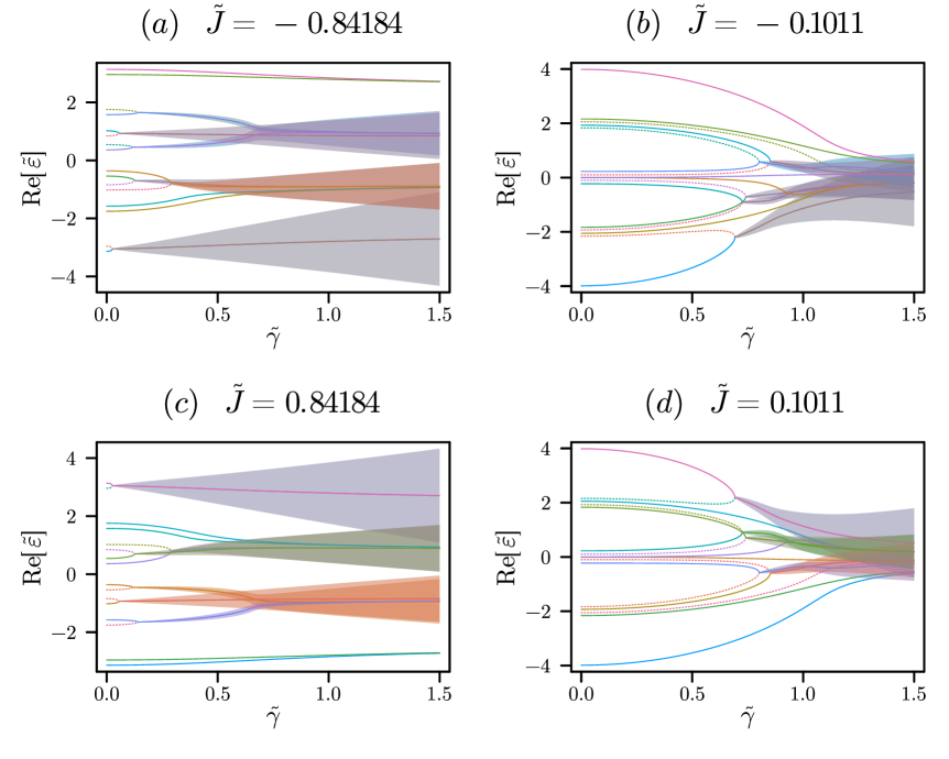
In Fig. 1, we present the results of the numerical diagonalization of the Hamiltonian (19) for an exemplary case of a chain of spins. The four subfigures display the dependence of the normalized eigenvalues on the normalized Ising coupling strength for different fixed values of . A complementary picture is presented in Fig. 2, where the four subfigures display the dependence of on for different fixed values of . We have computed the parities of all the states as explained in Appendix B and denoted them visually by solid (dotted) styles of lines. The pairs of the complex conjugated pairs are denoted by shaded ribbons. When two levels go through a second order EP, they form a complex conjugated pair. As such, the EPs can be identified in Figures by looking at the points where the ribbons end. Overall, the Figs. 1 and 2 very clearly demonstrate the -index selection rule in action.
IV.2.1 The ground state
Many of the features of the eigenspectrum are universal, i.e., they do not really depend neither on the chain length nor on the specific distribution of the imaginary longitudinal field (we can consider some other distributions that differ from the staggered one), as long as the Hamiltonian keeps -pseudo-Hermitian symmetry. One of such features is the formation of the EPs by the ground and the first excited states. For the antiferromagnetic sign of the interaction , the ground state always goes through the EP with the first excited state as becomes sufficiently large (see Fig. 1b-d). At the same time, for the ferromagnetic sign of the interaction , the ground state does not form EP point (see Fig. 1b-d). This fact has a simple explanation in terms of the parities of the states: for , both the ground and the first excited states has positive parities, while for , the first excited state has the negative parity. This can be also understood from the following argument. Let us focus on the strong-coupling limit . For the ferromagnetic coupling, the ground and the first excited states are symmetric and antisymmetric combinations of spin states and
| (21) | ||||
| (22) |
The parity operator (see Eq. (20)) exchanges the leftmost spin with the rightmost, the next-to-leftmost spin with the next-to-rightmost, etc. When we apply the parity operator to Eqs. (21) and (22), the both states and do not change sign. For the antiferromagnetic coupling, however, the ground and the first excited states have the form
| (23) | ||||
| (24) |
Although the ground state (23) still has the positive parity, the application of the parity operator to the state (24) flips the sign of the first excited state.
In Ref. [38], we have considered the ground state phase transitions in the limit for the periodic boundary conditions. We have argued there, that the phase transition into the ordered phase always happens via a second-order EP for the antiferromagnetic sign of the interaction, while for the ferromagnetic sign of the interaction the phase transition occurs without any EPs and the ground state energy stays real. The argument about the parities that we have just provided applies also to the case of the periodic boundary conditions. As a consequence, it serves as a clarification of the results of Ref. [38].
The atiferromagnetic symmetric and antisymmetric combinations (23) and (24) are the two highest-in-energy states for the ferromagnetic sign of the interaction, and vice versa. As such, the situation is reversed in comparison with the ground state: the two highest-in-energy states do not produce the EPs for the antiferromagnetic interaction, and go through a second-order EP for the ferromagnetic interaction (see Fig. 1b-d).
IV.2.2 Strong-coupling limit .
At , the Hamiltonian (19) is integrable, and it can be diagonalized analytically via the combination of Jordan-Wigner and generalized Bogolyubov transformations (see Appendix A and Ref. [39]). After diagonalization, the Hamiltonian (19) takes the form:
| (25) |
where and are the creation and annihilation operators of Bogolyubov-transformed fermionic modes.
In the strong-coupling limit, there are modes that form a band of width with the energies . There is also one almost zero fermionic mode with the exponentially small energy
| (26) |
Overall, the eigenspectrum is split into well isolated bands with the fixed number of excited non-zero fermionic modes. At the same time all the states form almost degenerate pairs. The two states in a pair differ by the filling of almost zero fermionic mode and the energy splitting is given by Eq. (26).
Using Eqs. (66) and (71), we can find the relative parity of the two levels forming an almost degenerate pair:
| (27) |
where is the number of excited non-zero fermionic modes. The labels and refer to “unoccupied” and “occupied” -mode respectively. For the case of the ferromagnetic coupling, almost degenerate pairs have opposite parities in every odd- band and identical parities in every even- band. For the case of the antiferromagnetic coupling, the situation is opposite: almost degenerate pairs have opposite parities in every even- band and identical parities in every odd- band (For the ground state one can put .)
Let us focus on one of the bands where the almost degenerate pairs have opposite parity. The almost degenerate pairs are well separated: the distance between different almost degenerate pairs is of the order , while the splitting inside the pair is exponentially small (see Eq. (26)). When considering a single almost degenerate pair, the influence of all the other states is negligible, and, similarly to the Section III, we expand the Hamiltonian at and obtain the matrix as is turned on:
| (28) |
where is identity matrix and
| (29) |
Comparing the general Eq. (18) with Eq. (28), we note that corresponds to , while . The diagonal matrix elements and from Eq. (18) are equal to zero in Eq. (28) because the diagonal matrix elements of the anti-Hermitian operator at are equal to zero.
The two eigenvalues of are
| (30) |
As we see, if the off-diagonal matrix element is not accidentally zero, the gap closes and the almost degenerate pair goes through a second-order EP at the critical value of which is linear in gap :
| (31) |
For larger values of , the eigenvalues form a complex conjugated pair. Since the gap is strongly diminished in the limit of large and/or , the second-order EPs appear already at extremely small values of .
Let us compare it with Figs. 2. Here, the strong-coupling limit corresponds to . The levels – form the first excited band while the levels - form the second excited band. In the first excited band of the ferromagnet (panel ) and the second excited band of the antiferromagnet (panel ) the almost degenerate pairs quickly go through second-order EPs and form complex conjugated pairs in accordance to our analysis.
In the second excited band of the ferromagnet and the first excited band of the antiferromagnet, the second-order EPs are formed only between the levels from different almost degenerate pairs, and some of the states do not form EPs at all (see states , in ferromagnet, , — in antiferromagnet).
IV.2.3 Weak-coupling limit
In this case, all the Bogolyubov-transformed fermionic modes form a band of width with the energies . So, all the eigenspectrum is divided into the bands with different total number of excited fermionic modes. However, there are no direct matrix elements of the anti-Hermitian part of the Hamiltonian between the states of the same band: The terms contributing to the anti-Hermitian part of the Hamiltonian consist of the odd number of fermionic creation and annihilation operators (see Eq. (43)). But the states with the same number of excited Bogolyubov-transformed fermionic modes are connected by an even number of fermionic creation and annihilation operators.
As a result, the second-order EPs are formed by the pairs of states belonging to different bands (see Figs. 2). Another consequence is that the eigenspectrum is overall more robust towards the formation of EPs.
IV.2.4 Intermediate coupling: stability of level crossings.
As we go from the weak-coupling limit to the strong-coupling limit at , the levels reorder themselves and the energy level crossings occur (see Fig. 1(a)). Let us discuss what happens with these crossings as is turned on.
At the crossing, the pair of levels is well isolated in energy from all the other levels, so yet again we apply the approach of Sections III and IV.2.2. Let us focus on the case of the opposite parities of the crossing levels (red dot in Fig. 1(a) is an example). At , we can write the projected Hamiltonian in the vicinity of the crossing point as
| (32) |
where is identity matrix and parameter measures the detuning from the crossing point. When we add small , the projected Hamiltonian becomes (see Eqs. (18) and (28))
| (33) |
The two eigenvalues in this case are
| (34) |
At finite , the crossing is split into two second-order EPs at . For the eigenvalues are real, while in between the two EPs , the two eigenvalues form a complex conjugated pair.
This is precisely what happens with the opposite parity crossings in Fig. 1. As an example, we have singled out one of such crossings in panel and marked it with a red dot. In panel , we have marked the two corresponding EPs after splitting by red dots as well.
In the case of same parity crossing, the transformation of the exact crossing point into the EP is strictly forbidden. Moreover, the off-diagonal matrix element at is equal to zero, i.e., in linear in order, the gap at the same parity crossing does not open. However, when we go to finite , the general form of the projected Hamiltonian (18) does not exclude the possibility of generation of off-diagonal matrix elements. If such matrix elements were to appear, it would lead to avoided crossings and opening of the gap [53, 54].
It is noteworthy, that in the model we considered, the same parity crossings are stable and do not open gaps. As an example, we have marked one of such crossings with a black dot in Figs. 1. We argue that it is a consequence of the special structure of the anti-Hermitian part of the Hamiltonian (19): as we have mentioned in Section IV.2.3, it consists only of the terms that are odd in the number of fermionic operators. We have experimented with the different distributions of the imaginary field. For example, we have considered a staggered imaginary transverse field (Song’s model [50]) and a staggered imaginary field with both transverse and longitudinal components. In the former case, the anti-Hermitian part of the Hamiltonian consists only of even in fermionic operators terms, and the same parity states form stable exact crossings. In the latter case, however, we saw the gaps opening because of avoided crossing. Overall, this topic voids further exploration in a future work.
IV.3 The eigenspectrum: third-order EPs.
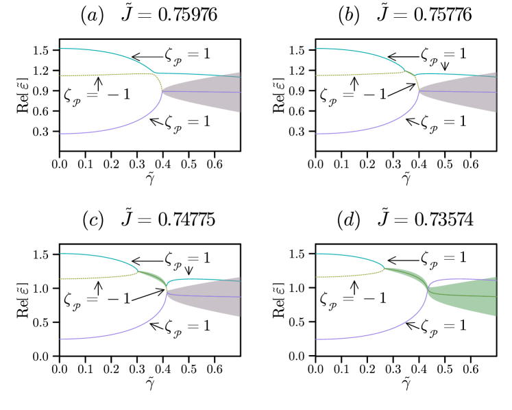
For larger values of , the two exception points of the second order can coalesce and go through the exception point of the third order (EP3) [55, 56] as seen in Fig. 1(c,d) and insets therein. To clarify the structure of EP3, we provide the complementary picture in Fig. 3, where we display the normalized eigenvalues of the levels forming the highlighted EP3 as the functions of for different values of . The parities of the levels are denoted both by annotations and by differing line styles. The EP3 is formed by three nearby levels, where the lower and the upper levels have the same parity index, while the middle level has the opposite parity index. The middle level is allowed to form a complex conjugated pair with either of the other two levels, while it is disallowed by selection rule for the lower and the upper level. As a result, the vicinity of EP3 is characterized by the competition between these two possible pairings of the middle level. For example, for larger values of (see Fig. 3(a)), the upper level’s eigenvalue stays real, while the middle and the lower levels form a complex conjugated pair. On the contrary, for smaller values of (see Fig. 3(d)) the situation is opposite. An interesting consequence of EP3, is that for larger values of , there is an abrupt exchange between the upper and lower levels as is varied (compare panels (c) and (d) of Fig. 3). This is consistent with the jumps visible in the insets of Fig. 1(c,d) and is attributed to the branching nature of the singularity at EP3.
When the value is increased even further, the system passes through an increasing number of third-order EPs at different values of . In this section, we focused on a particular third-order EP. All the other third-order EPs that we have observed in the system, have the same structure that we have just described: coalescing pair of second-order EPs with shared level of opposite parity.
V Discussion and Conclusion
In this paper, we have theoretically studied the formation of Exceptional Points (EPs) in the eigenpectrum of a Hamiltonian with pseudo-Hermitian (psH) symmetry as the strength of Hermiticity-breaking terms increases.
We have shown, that for an overall non-degenerate level with real eigenvalue, the left and the right eigenvectors can always be rescaled to satisfy
| (35) |
where
| (36) |
The -index is conserved in the whole region of parameters where the level has real eigenvalue and coincides with the signs of the eigenvalues of the pseudometric operator when anti-Hermitian part of the Hamiltonian is zero. After that, we have shown that the formation of a second-order EP is governed by index-based selection rule: the formation of EP is impossible for a pair of levels with identical -indices.
To clearly illustrate these ideas, we have considered a transverse-field Ising spin chain with imaginary staggered longitudinal field, which has pseudo-Hermitian symmetry with respect to the parity operator. In this case, the index coincides with the parity of a state at vanishing imaginary field. The system is integrable in the absence of Hermiticity-breaking terms, which enabled us to compute the parities of all the levels analytically. Using the knowledge of the level parities, we have applied the selection rule to analyse second-order EP formation in the strong- and the weak-coupling limits, as well as the stablity of level crossings with respect to Hermiticity-breaking terms. It is noteworthy, that in the considered model, the selection rule for EP formation is very similar to the selection rule that governs avoided crossing, although the condition on the parities is reversed [53]: the avoided crossing happens when the parities are identical, while EP formation — when they are opposite.
We have also demonstrated, how the third-order EPs can be obtained by tuning two second-order EPs with shared level of opposite -index to coincide. In principle, a fourth-order EP can be obtained by tuning two third-order EPs with shared levels, a fifth-order EP — by tuning two fourth-order EP with shared levels, etc.. As a consequence of the selection rule, a higher-order EP in a psH-symmetric system must be formed by the levels with staggered signature of -indices.
Moreover, the analysis of the paper goes beyond the specific shape of the anti-Hermitian term we considered. In principle, it stays relevant even for general form of anti-Hermitian terms, as long as they preserve pseudo-Hermitian symmetry. This is attributed to the fact, that the parity signature of the levels significantly limits the possible structure of the eigenspectrum.
For example, one could consider a more general distribution of the imaginary longitudinal field:
| (37) |
This introduces additional independent control parameters which is necessary to tune the system to higher-order EPs. If we require that , then the Hamiltonian stays both -symmetric and -psH-symmetric.
In Section II, we did not really specify the nature of the parameters . In principle, one can consider to be a Bloch Hamiltonian of some extended system, where the vector of parameters contains the Bloch wave-vector as part of its components. It follows from the fact that pseudo-Hermitian symmetry does not change the wave-vector [28], so it acts as the internal symmetry of the Bloch Hamiltonian. It is potentially interesting to apply the analysis of the paper to the non-Hermitian topological systems.
Let us finally mention that the instabilities of psH-symmetric Hamiltonians were systematically studied in 50-s by the Soviet mathematicians Krein [57] and Gel’fand with Lidskii [58] in the context of linear differential equations with periodic coefficients. A consistent recollection of their works can be found in the book [59]. They defined a pseudo-scalar product
| (38) |
which was then used to classify all the real eigenvalues of the Hamiltonian as first, second and mixed kind depending on the signature of the restriction of this pseudo-scalar product to the corresponding eigensubspace: positive definite, negative definite and undefinite respectively. After that they have shown, that the eigenvalues of the first and second kind are stable with respect to the perturbations of the Hamiltonian, while the mixed kind eigenvalues can branch off into complex conjugated pairs.
Acknowledgements
We acknowledge the financial support of Deutsche Forschungsgemeinschaft (Projekt EF 11/10-1) and the financial support through the European Union’s Horizon 2020 research and innovation program under grant agreement No 863313 ’Supergalax’.
Appendix A Exact Diagonalization via Jordan-Wigner transformation.
Introducing the raising and the lowering operators , we define the Jordan-Wigner fermionic operators:
| (39) |
Inverting this definition, we can write the spin operators as
| (40) |
Substituting it into the Hamiltonian (19) with open boundary conditions, we find
| (41) | ||||
| (42) | ||||
| (43) |
As we see, the terms contributing to the non-Hermitian part of the Hamiltonian contain odd numbers of fermionic operators ranging from 1 operator ( term) to operators ( term). As a result, it is impossible to exactly daigonalize the Hamiltonian (41) at .
For , the Hamiltonian and the quadratic form over the fermionic operators can be diagonalized via a generalized Bogolyubov transformation [39]:
| (44) |
where and are the new fermionic creation and annihilation operators:
| (45) | ||||
| (46) |
The energies and the vectors and are determined as the eigenvalues and the eigenvectors of certain matrices, composed from the coefficients of the Hamiltonian. Here, we don’t go through the details, and only list the final results for this variables. We can refer the interested reader to Appendix A and Section IIID of [39].
The energies are
| (47) |
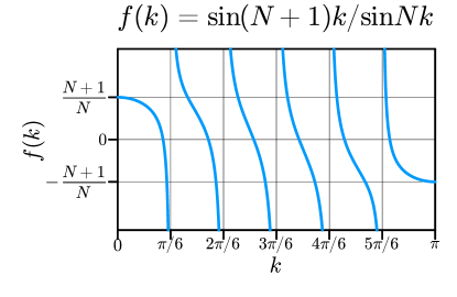
where the wave vectors are determined as the solutions of the equation
| (48) |
The complete set of corresponds to the interval . We display the plot of the function for in Fig. 4. The equation (48) can be solved graphically by finding the intersections of the horizontal line with the curve .
The vectors and have the form
| (49) |
Here, are the normalization factors which are of no importance to us. The factors determine the parities of the Bogolyubov-transformed fermionic modes and are equal to
| (50) |
There is a symmetry between the fermionic modes energies in the cases of ferromagnet and antiferromagnet. As the left-hand side of Eq. (48) satisfies , if is the wave vector of the fermionic mode in the case of the ferromagnet, then is the wave vector of the fermionic mode in the case of antiferromagnet. From Eq. (47) if follows then that the energies of these modes are identical.
Overall, it is convenient to label the wave vectors as in the order of the increasing energy. In the case of ferromagnet, it means that (consider graphical solution of Eq. (48) with the help of Fig. 4)
| (51) |
while in the case of antiferromagnet it implies
| (52) |
Notice, that as we move from ferromagnet to antiferromagnet, the order of the modes is reversed, which is reflected in Fig. (1)(a).
Finally, we should discuss the properties of the mode, which is responsible for the paramagnet-(anti)ferromagnet transition in the tranverse-field Ising chain. For , the wave-vector turns complex:
| (53) | ||||
| (54) |
where satisfies
| (55) |
The corresponding energy decays exponentially with the system size for large :
| (56) |
For , the ground state becomes doubly degenerate in the thermodynamic limit which corresponds to the two degenerate vacua in the -broken phase.
Appendix B Determination of the parities of all the states at .
In this appendix, we are going to show how the parities of all the states can be obtained in the closed form in the absence of imaginary longitudinal magnetic field. In order to do that, we are going to build upon the notions introduced in A. The reader can also skip the derivation straight to B.3 to see the final results.
B.1 Recursion formula.
The action of the parity symmetry on the spin operators is defined as (see Eq. (20))
| (57) |
For the Jordan-Wigner fermionic creation and annihilation operators (see Eq. (39)), however, the action of the parity symmetry is complicated by the fact, that the string of the spin operators gets reattached to the right end of the chain:
| (58) |
In order to reattach the spin string back to the left end of the chain, let us introduce the full spin string operator:
| (59) |
The square of is an identity operator, so let us multiply Eq. (58) on the right with an identity operator:
| (60) |
where we have used the identity
| (61) |
This way, we can define the action of parity symmetry on bare fermionic creation and annihilation operators as
| (62) |
Substituting these identities into Eq. (45), we find the action of the parity symmetry on the creation operator of Bogolyubov-transformed fermionic mode:
| (63) |
In the penultimate equality, we have used the identity
| (64) |
which follows directly from the explicit form of the vectors and (see Eq. (49)). We can also repeat the same steps for the annihilation operator to find
| (65) |
With the knowledge of the transformation properties of the creation operator , the parities of all the states can be found by induction. Each state is completely determined by the set of occupied Bogolyubov-transformed fermionic modes. Let be a state with excited fermionic modes and parity . Let us also assume that the mode with the wave vector is unoccupied in the state . Then, if we add this mode to the state, we obtain
| (66) |
The spin string operator is equal to for the states with an even number of original Jordan-Wigner fermions, while it is for the states with an odd number of original Jordan-Wigner fermions. The eigenstates of the transverse-field Ising Hamiltonian (44) mix the states with the different number of original Jordan-Wigner fermions. However, these eigenstates has definite evenness/oddness. For example, the ground state is even. (This can be confirmed by directly computing and showing that it is equal to . See [39] for the details of such a copmutation.) As such, , which we used in the last equality of Eq. (66).
B.2 Parity factors of Bogolyubov-transformed fermionic modes.
As we see, in order to compute the parities, we need to determine the factors first. If , then . Correspondingly, if , then . Substituting it into Eq. (50), we find
| (67) |
in the case of ferromagnet and
| (68) |
in the case of antiferromagnet. Here, we have used the labeling of the Bogolyubov-transformed fermionic modes introduced in A and Eqs. (51) and (52).
If the wave-vector of the lowest energy mode turns complex, then in the case of ferromagnet, we have
| (69) |
while in the case of antiferromagnet,
| (70) |
Here, we have used Eqs. (53) and (54). Note that the resulting factors are consistent with Eqs. (67) and (68). Overall, we can combine Eqs. (67) and (68) together to get
| (71) |
B.3 Final results.
Let us consider the state with excited Bogolyubov-transformed modes, which have wave-vectors :
| (72) |
As we have discussed in Section IV.2.1 of the main text, the ground state has even parity. By repeatedly applying Eq. (66) to the ground state, we find the parity of the state :
| (73) |
where the factors are given by Eq. (71).
We can also use Eq. (66) to determine the relative sign of the parities of the two states. For example, let us consider the ground state and the first excited state . The first excited state is obtained by exciting the lowest energy Bogolyubov-transoformed fermionic mode:
| (74) |
Using Eqs. (66) and (71), we find for a lattice with even
| (75) |
Analogously, we can consider the next-to-highest and the highest levels:
| (76) |
Since the next-to-highest level has excited Bogolyubov-transformed fermionic modes,
| (77) |
References
- Acín et al. [2018] A. Acín, I. Bloch, H. Buhrman, T. Calarco, C. Eichler, J. Eisert, D. Esteve, N. Gisin, S. J. Glaser, F. Jelezko, et al., The quantum technologies roadmap: a european community view, New Journal of Physics 20, 080201 (2018).
- Mooij et al. [1999] J. Mooij, T. Orlando, L. Levitov, L. Tian, C. H. Van der Wal, and S. Lloyd, Josephson persistent-current qubit, Science 285, 1036 (1999).
- Xiao et al. [2019] Y.-X. Xiao, Z.-Q. Zhang, Z. H. Hang, and C. T. Chan, Anisotropic exceptional points of arbitrary order, Phys. Rev. B 99, 241403 (2019).
- Ding et al. [2022] K. Ding, C. Fang, and G. Ma, Non-hermitian topology and exceptional-point geometries, Nature Reviews Physics 4, 745 (2022).
- Bergholtz et al. [2021] E. J. Bergholtz, J. C. Budich, and F. K. Kunst, Exceptional topology of non-hermitian systems, Rev. Mod. Phys. 93, 015005 (2021).
- Hu et al. [2022] H. Hu, S. Sun, and S. Chen, Knot topology of exceptional point and non-hermitian no-go theorem, Phys. Rev. Res. 4, L022064 (2022).
- Wiersig [2014] J. Wiersig, Enhancing the sensitivity of frequency and energy splitting detection by using exceptional points: Application to microcavity sensors for single-particle detection, Phys. Rev. Lett. 112, 203901 (2014).
- Wiersig [2016] J. Wiersig, Sensors operating at exceptional points: General theory, Phys. Rev. A 93, 033809 (2016).
- Chen et al. [2017] W. Chen, Ş. K. Özdemir, G. Zhao, J. Wiersig, and L. Yang, Exceptional points enhance sensing in an optical microcavity, Nature 548, 192 (2017).
- Hokmabadi et al. [2019] M. P. Hokmabadi, A. Schumer, D. N. Christodoulides, and M. Khajavikhan, Non-hermitian ring laser gyroscopes with enhanced sagnac sensitivity, Nature 576, 70 (2019).
- Dembowski et al. [2004] C. Dembowski, B. Dietz, H.-D. Gräf, H. L. Harney, A. Heine, W. D. Heiss, and A. Richter, Encircling an exceptional point, Phys. Rev. E 69, 056216 (2004).
- Gilary et al. [2013] I. Gilary, A. A. Mailybaev, and N. Moiseyev, Time-asymmetric quantum-state-exchange mechanism, Phys. Rev. A 88, 010102 (2013).
- Ghosh and Chong [2016] S. N. Ghosh and Y. D. Chong, Exceptional points and asymmetric mode conversion in quasi-guided dual-mode optical waveguides, Scientific Reports 6, 10.1038/srep19837 (2016).
- Doppler et al. [2016] J. Doppler, A. A. Mailybaev, J. Böhm, U. Kuhl, A. Girschik, F. Libisch, T. J. Milburn, P. Rabl, N. Moiseyev, and S. Rotter, Dynamically encircling an exceptional point for asymmetric mode switching, Nature 537, 76 (2016).
- Zhang et al. [2018] X.-L. Zhang, S. Wang, B. Hou, and C. T. Chan, Dynamically encircling exceptional points: In situ control of encircling loops and the role of the starting point, Phys. Rev. X 8, 021066 (2018).
- Laha et al. [2018] A. Laha, A. Biswas, and S. Ghosh, Nonadiabatic modal dynamics around exceptional points in an all-lossy dual-mode optical waveguide: Toward chirality-driven asymmetric mode conversion, Phys. Rev. Appl. 10, 054008 (2018).
- Laha and Ghosh [2017] A. Laha and S. Ghosh, Connected hidden singularities and toward successive state flipping in degenerate optical microcavities, Journal of the Optical Society of America B 34, 238 (2017).
- Laha et al. [2017] A. Laha, A. Biswas, and S. Ghosh, Next-nearest-neighbor resonance coupling and exceptional singularities in degenerate optical microcavities, Journal of the Optical Society of America B 34, 2050 (2017).
- Laha et al. [2019] A. Laha, A. Biswas, and S. Ghosh, Minimally asymmetric state conversion around exceptional singularities in a specialty optical microcavity, Journal of Optics 21, 025201 (2019).
- Brandstetter et al. [2014] M. Brandstetter, M. Liertzer, C. Deutsch, P. Klang, J. Schöberl, H. E. Türeci, G. Strasser, K. Unterrainer, and S. Rotter, Reversing the pump dependence of a laser at an exceptional point, Nature Communications 5, 10.1038/ncomms5034 (2014).
- Wong et al. [2016] Z. J. Wong, Y.-L. Xu, J. Kim, K. O'Brien, Y. Wang, L. Feng, and X. Zhang, Lasing and anti-lasing in a single cavity, Nature Photonics 10, 796 (2016).
- Hodaei et al. [2017] H. Hodaei, A. U. Hassan, S. Wittek, H. Garcia-Gracia, R. El-Ganainy, D. N. Christodoulides, and M. Khajavikhan, Enhanced sensitivity at higher-order exceptional points, Nature 548, 187 (2017).
- Laha et al. [2020a] A. Laha, D. Beniwal, S. Dey, A. Biswas, and S. Ghosh, Third-order exceptional point and successive switching among three states in an optical microcavity, Phys. Rev. A 101, 063829 (2020a).
- Laha et al. [2021] A. Laha, D. Beniwal, and S. Ghosh, Successive switching among four states in a gain-loss-assisted optical microcavity hosting exceptional points up to order four, Phys. Rev. A 103, 023526 (2021).
- Li et al. [2022] Z.-Z. Li, W. Chen, M. Abbasi, K. W. Murch, and K. B. Whaley, Speeding up entanglement generation by proximity to higher-order exceptional points (2022).
- Delplace et al. [2021] P. Delplace, T. Yoshida, and Y. Hatsugai, Symmetry-protected multifold exceptional points and their topological characterization, Phys. Rev. Lett. 127, 186602 (2021).
- Stålhammar and Bergholtz [2021] M. Stålhammar and E. J. Bergholtz, Classification of exceptional nodal topologies protected by symmetry, Phys. Rev. B 104, L201104 (2021).
- Sayyad and Kunst [2022a] S. Sayyad and F. K. Kunst, Realizing exceptional points of any order in the presence of symmetry, Phys. Rev. Res. 4, 023130 (2022a).
- Sayyad and Kunst [2022b] S. Sayyad and F. K. Kunst, Realizing exceptional points of any order in the presence of symmetry, Phys. Rev. Res. 4, 023130 (2022b).
- Mostafazadeh [2002a] A. Mostafazadeh, Pseudo-hermiticity versus pt symmetry: the necessary condition for the reality of the spectrum of a non-hermitian hamiltonian, Journal of Mathematical Physics 43, 205 (2002a).
- Mostafazadeh [2002b] A. Mostafazadeh, Pseudo-hermiticity versus pt-symmetry. ii. a complete characterization of non-hermitian hamiltonians with a real spectrum, Journal of Mathematical Physics 43, 2814 (2002b).
- Mostafazadeh [2002c] A. Mostafazadeh, Pseudo-hermiticity versus pt-symmetry iii: Equivalence of pseudo-hermiticity and the presence of antilinear symmetries, Journal of Mathematical Physics 43, 3944 (2002c).
- Mostafazadeh [2010a] A. Mostafazadeh, Pseudo-hermitian representation of quantum mechanics, International Journal of Geometric Methods in Modern Physics 7, 1191 (2010a).
- Ashida et al. [2020] Y. Ashida, Z. Gong, and M. Ueda, Non-hermitian physics, Advances in Physics 69, 249 (2020).
- Zhang et al. [2020] R. Zhang, H. Qin, and J. Xiao, PT-symmetry entails pseudo-hermiticity regardless of diagonalizability, Journal of Mathematical Physics 61, 012101 (2020).
- Bian et al. [2020] Z. Bian, L. Xiao, K. Wang, X. Zhan, F. A. Onanga, F. Ruzicka, W. Yi, Y. N. Joglekar, and P. Xue, Conserved quantities in parity-time symmetric systems, Physical Review Research 2, 022039 (2020).
- Agarwal et al. [2022] K. S. Agarwal, J. Muldoon, and Y. N. Joglekar, Conserved quantities in non-hermitian systems via vectorization method, arXiv preprint arXiv:2201.05019 (2022).
- Starkov et al. [2022] G. A. Starkov, M. V. Fistoul, and I. M. Eremin, Quantum phase transitions in non-hermitian -symmetric transverse-field ising spin chains (2022).
- Lieb et al. [1961] E. Lieb, T. Schultz, and D. Mattis, Two soluble models of an antiferromagnetic chain, Annals of Physics 16, 407 (1961).
- Ding et al. [2021] L. Ding, K. Shi, Q. Zhang, D. Shen, X. Zhang, and W. Zhang, Experimental determination of p t-symmetric exceptional points in a single trapped ion, Physical Review Letters 126, 083604 (2021).
- Lourenço et al. [2022] J. A. Lourenço, G. Higgins, C. Zhang, M. Hennrich, and T. Macrì, Non-hermitian dynamics and pt-symmetry breaking in interacting mesoscopic rydberg platforms, Physical Review A 106, 023309 (2022).
- Li et al. [2019] J. Li, A. K. Harter, J. Liu, L. de Melo, Y. N. Joglekar, and L. Luo, Observation of parity-time symmetry breaking transitions in a dissipative floquet system of ultracold atoms, Nature communications 10, 1 (2019).
- Cartarius and Wunner [2012] H. Cartarius and G. Wunner, Model of a pt-symmetric bose-einstein condensate in a -function double-well potential, Physical Review A 86, 013612 (2012).
- Naghiloo et al. [2019] M. Naghiloo, M. Abbasi, Y. N. Joglekar, and K. Murch, Quantum state tomography across the exceptional point in a single dissipative qubit, Nature Physics 15, 1232 (2019).
- Dogra et al. [2021] S. Dogra, A. A. Melnikov, and G. S. Paraoanu, Quantum simulation of parity–time symmetry breaking with a superconducting quantum processor, Communications Physics 4, 1 (2021).
- Wu et al. [2019] Y. Wu, W. Liu, J. Geng, X. Song, X. Ye, C.-K. Duan, X. Rong, and J. Du, Observation of parity-time symmetry breaking in a single-spin system, Science 364, 878 (2019).
- Tetling et al. [2022] L. Tetling, M. Fistul, and I. M. Eremin, Linear response for pseudo-hermitian hamiltonian systems: Application to pt-symmetric qubits, Physical Review B 106, 134511 (2022).
- Mostafazadeh [2010b] A. Mostafazadeh, Pseudo-Hermitian Representation of Quantum Mechanics, International Journal of Geometric Methods in Modern Physics 07, 1191 (2010b).
- Dirac [1930] P. A. M. Dirac, The Principles of Quantum Mechanics (Clarendon Press, 1930).
- Li et al. [2014] C. Li, G. Zhang, X. Z. Zhang, and Z. Song, Conventional quantum phase transition driven by a complex parameter in a non-hermitian ising model, Phys. Rev. A 90, 012103 (2014).
- Li and Song [2015] C. Li and Z. Song, Finite-temperature quantum criticality in a complex-parameter plane, Phys. Rev. A 92, 062103 (2015).
- Lenke et al. [2021] L. Lenke, M. Mühlhauser, and K. P. Schmidt, High-order series expansion of non-hermitian quantum spin models, Phys. Rev. B 104, 195137 (2021).
- Neumann and Wigner [1929] J. v. Neumann and E. Wigner, Über das verhalten von eigenwerten bei adiabatischen prozessen, Physikalische Zeitschrift 30, 467 (1929).
- Grifoni and Hänggi [1998] M. Grifoni and P. Hänggi, Driven quantum tunneling, Physics Reports 304, 229 (1998).
- Laha et al. [2020b] A. Laha, D. Beniwal, S. Dey, A. Biswas, and S. Ghosh, Third-order exceptional point and successive switching among three states in an optical microcavity, Phys. Rev. A 101, 063829 (2020b).
- Mandal and Bergholtz [2021] I. Mandal and E. J. Bergholtz, Symmetry and higher-order exceptional points, Phys. Rev. Lett. 127, 186601 (2021).
- Krein [1950] M. Krein, A generalization of some investigations of linear differential equations with periodic coefficients, in Doklady Akad. Nauk SSSR, Vol. 73 (1950) pp. 445–448.
- Gel’fand and Lidskii [1955] I. M. Gel’fand and V. B. Lidskii, On the structure of the regions of stability of linear canonical systems of differential equations with periodic coefficients, Uspekhi Matematicheskikh Nauk 10, 3 (1955).
- Starzhinskii and Yakubovich [1975] V. Starzhinskii and V. Yakubovich, Linear differential equations with periodic coefficients 2 vol. (Wiley London, 1975).