Balanced Training for Sparse GANs

Abstract

Over the past few years, there has been growing interest in developing larger and deeper neural networks, including deep generative models like generative adversarial networks (GANs). However, GANs typically come with high computational complexity, leading researchers to explore methods for reducing the training and inference costs. One such approach gaining popularity in supervised learning is dynamic sparse training (DST), which maintains good performance while enjoying excellent training efficiency. Despite its potential benefits, applying DST to GANs presents challenges due to the adversarial nature of the training process. In this paper, we propose a novel metric called the balance ratio (BR) to study the balance between the sparse generator and discriminator. We also introduce a new method called balanced dynamic sparse training (ADAPT), which seeks to control the BR during GAN training to achieve a good trade-off between performance and computational cost. Our proposed method shows promising results on multiple datasets, demonstrating its effectiveness. Our code is available at https://github.com/YiteWang/ADAPT.

1 Introduction

Generative adversarial networks (GANs) (Goodfellow et al., 2020; Brock et al., 2018; Sauer et al., 2022; Lee et al., 2022) are a type of generative model that has gained significant attention in recent years due to their impressive performance in image-generation tasks. However, the mainstream models in GANs are known to be computationally intensive, making them challenging to train in resource-constrained settings. Therefore, it is crucial to develop methods that can effectively reduce the computational cost of training GANs while maintaining their performance, making GANs more practical and applicable in real-world scenarios.

Neural network pruning has recently emerged as a powerful tool to reduce the training and inference costs of DNNs for supervised learning. There are mainly three genres of pruning methods, namely pruning-at-initialization, pruning-during-training, and post-hoc pruning methods. Post-hoc pruning (Janowsky, 1989; LeCun et al., 1989; Han et al., 2015) can date back to the 1980s, which was first introduced for reducing inference time and memory requirements for efficient deployment; hence does not align with our purpose of efficient training. Later, pruning-at-initialization (Lee et al., 2018; Wang et al., 2020a; Tanaka et al., 2020) and pruning-during-training methods (Wen et al., 2016) were introduced to circumvent the need to fully train the dense networks. However, early pruning-during-training algorithms (Louizos et al., 2017) do not bring much training efficiency compared to post-hoc pruning, while pruning-at-initialization methods usually suffer from significant performance drop (Frankle et al., 2021). Recently, advances in dynamic sparse training (DST) (Mocanu et al., 2018; Evci et al., 2020; Liu et al., 2021a, b, c) for the first time show that pruning-during-training methods can have comparable training FLOPs as pruning-at-initialization methods while having competing performance to post-hoc pruning. Therefore, applying DST on GANs seems to be a promising choice.

Although DST has attained remarkable achievements in supervised learning, the application of DST on GANs is not successful due to newly emerging challenges. One challenge is keeping the generator and the discriminator balanced. In particular, using overly strong discriminators can lead to overfitting, while weaker discriminators may fail to effectively prevent mode collapse (Arora et al., 2017; Bai et al., 2018). Hence, balancing the sparse generator and the (possibly) sparse discriminator throughout training is even more difficult. To mitigate the unbalance issue, a recent work STU-GAN (Liu et al., 2022) proposes to apply DST directly to the generator. However, we find empirically that such an algorithm is likely to fail when the generator is already more powerful than the discriminator. Consequently, it remains unclear how to conduct balanced dynamic sparse training for GANs.

To this end, we propose a metric called balance ratio (BR), which measures the degree of balance of the two components, to study sparse GAN training. We find that BR is useful in (1) understanding the interaction between the discriminator and the generator, (2) identifying the cause of a certain training failure/collapse (Brock et al., 2018; Chen et al., 2021a), and (3) helping stabilize sparse GAN training as an indicator. To our best knowledge, this is the first study to quantify the unbalance of sparse GANs and may even provide new insights into dense GAN training.

Furthermore, using BR as an indicator, we propose bAlanced DynAmic sParse Training (ADAPT) to adjust the density and the connections of the discriminator automatically during training.

Our main contributions are summarized below:

• We introduce a novel quantity named balance ratio to study the degree of balance in sparse GAN training.

• We find empirically that the balance ratio is problematic in certain practical training scenarios and that existing methods are inadequate for resolving this issue.

• We propose ADAPT, which makes real-time monitoring of the balance ratio. By dynamically adjusting the discriminator, ADAPT enables effective control of the balance ratio throughout training. Empirically, ADAPT achieves a good trade-off between performance and computational cost on several datasets.

2 Related works

2.1 Neural network pruning

In deep learning, efficiency is achieved through several methods. This paper primarily focuses on model training and inference efficiency, which is different from techniques for data efficiency (Wang et al., 2018b; Wu et al., 2023a, b). These include neural architecture search (NAS) (Wang et al., 2022a; Liu et al., 2018a) to discover optimal network structures, quantization (Hubara et al., 2017; Rastegari et al., 2016) for computational efficacy, knowledge distillation (Hinton et al., 2015) to leverage the knowledge of larger models for smaller counterparts, and neural network pruning to remove unnecessary connections. Among these, neural network pruning is the focal point of our research. More specifically, we narrow our focus on unstructured pruning (Han et al., 2015; Frankle and Carbin, 2018), where individual weight is the finest resolution. This contracts with structured pruning (Liu et al., 2017; Luo et al., 2017; Liu et al., 2018b; Huang and Wang, 2018) where entire neurons or channels are pruned.

Post-hoc pruning. Post-hoc pruning method prunes weights of a fully-trained neural network. It usually requires high computational costs due to the multiple rounds of the train-prune-retrain procedure (Han et al., 2015; Renda et al., 2020). Some use specific criteria (LeCun et al., 1989; Hassibi et al., 1993; Han et al., 2015; Guo et al., 2016; Dong et al., 2017; Dai et al., 2018; Yu et al., 2018; Molchanov et al., 2019) to remove weights, while others perform extra optimization iterations (Verma and Pesquet, 2021). Post-hoc pruning was initially proposed to reduce the inference time, while lottery ticket works (Frankle and Carbin, 2018; Renda et al., 2020) aimed to mine trainable sub-networks.

Pruning-at-initialization methods. SNIP (Lee et al., 2018) is one of the pioneering works that aim to find trainable sub-networks without any training. Some follow-up works (Wang et al., 2020a; Tanaka et al., 2020; de Jorge et al., 2020; Patil and Dovrolis, 2021; Alizadeh et al., 2022) aim to propose different metrics to prune networks at initialization. Among them, Synflow (Tanaka et al., 2020), SPP (Lee et al., 2019), and FORCE (de Jorge et al., 2020) try to address the problem of layer collapse during pruning. NTT (Liu and Zenke, 2020), PHEW (Patil and Dovrolis, 2021), and NTK-SAP (Wang et al., 2022b) draw inspiration from neural tangent kernel theory.

Pruning-during-training methods. Another genre of pruning algorithms prunes or adjusts DNNs throughout training. Early works add explicit $\ell_{0}$ (Louizos et al., 2017) or $\ell_{1}$ (Wen et al., 2016) regularization terms to encourage a sparse solution, hence mitigating performance drop incurred by post-hoc pruning. Later works learn the subnetworks structures through projected gradient descent (Zhou et al., 2021) or trainable masks (Srinivas et al., 2017; Xiao et al., 2019; Kang and Han, 2020; Kusupati et al., 2020; Liu et al., 2020; Savarese et al., 2020). However, these pruning-during-training methods often do not introduce memory sparsity during training. As a remedy, DST methods (Bellec et al., 2017; Mocanu et al., 2018; Mostafa and Wang, 2019; Dettmers and Zettlemoyer, 2019; Evci et al., 2020; Liu et al., 2021a, b, c; Graesser et al., 2022) were introduced to train the neural networks under a given parameter budget while allowing mask change during training.

2.2 Generative adversarial networks

Generative adversarial networks (GANs). GANs (Goodfellow et al., 2020) have drawn considerable attention and have been widely investigated for years. Deep convolutional GANs (Radford et al., 2015) replace fully-connected layers in the generator and the discriminator. Follow-up works (Gulrajani et al., 2017; Karras et al., 2017; Brock et al., 2018; Zhang et al., 2019) employed more advanced methods to improve the fidelity of generated samples. After that, several novel loss functions (Salimans et al., 2016; Mao et al., 2017; Arjovsky et al., 2017; Gulrajani et al., 2017; Sun et al., 2020), normalization and regularization methods (Miyato et al., 2018; Terjék, 2019; Wu et al., 2021) were proposed to stabilize the adversarial training. Besides the efforts devoted to training GANs, image-to-image translation is also extensively explored (Zhu et al., 2017b, a; Choi et al., 2018; Karras et al., 2020b; Ledig et al., 2017; Wang et al., 2018a).

GAN balance. Addressing the balance between the generator and discriminator in GAN training has been the focus of various works. However, directly applying existing methods to sparse GAN training poses challenges. For instance, (Arora et al., 2017; Bai et al., 2018) offer theoretical analyses on the issue of imbalance but may have limited practical benefits, e.g., they require training multiple generators and discriminators. Empirically, BEGAN (Berthelot et al., 2017) proposes to use proportional control theory to maintain a hyper-parameter $\frac{\mathbb{E}[|G(z)-D(G(z))|^{\eta}]}{\mathbb{E}[|x-D(x)|^{\eta}]}$, but it is only applicable when the discriminator is an auto-encoder. Unbalanced GAN (Ham et al., 2020) pretrains a VAE to initialize the generator, which may only address the unbalance near initialization. GCC (Li et al., 2021) considers the balance during GAN compression, while its criterion requires a trained (dense) GAN, which is not given in the DST setting. Finally, STU-GAN (Liu et al., 2022) proposes to use DST to address the unbalance issues but may fail under certain conditions, as demonstrated in our experiments.

GAN compression and pruning. One of the promising ways is based on neural architecture search and distillation algorithm (Li et al., 2020; Fu et al., 2020; Hou et al., 2021). Another part of the work applied pruning-based methods for generator compression (Shu et al., 2019; Yu and Pool, 2020; Jin et al., 2021). Later, works by (Wang et al., 2020b) presented a unified framework by combing the methods mentioned above. Nevertheless, they only focus on the pruning of generators, thus potentially posing a negative influence on Nash Equilibrium between generators and discriminators. GCC (Li et al., 2021) compresses both components of GANs by letting the student GANs also learn the losses. Another line of work (Kalibhat et al., 2021; Chen et al., 2021b, a) tries to test the existence of lottery tickets in GANs. To the best of our knowledge, STU-GAN (Liu et al., 2022) is the only work that tries to directly train sparse GANs from scratch.

3 Preliminary and setups

Generative adversarial networks (GANs) have two fundamental components, a generator $G(\cdot;\bm{\theta}_{G})$ and a discriminator $D(\cdot;\bm{\theta}_{D})$. Specifically, the generator maps a sampled noise $\bm{z}$ from a multivariate normal distribution $p(\bm{z})$ into a fake image to cheat the discriminator. In contrast, the discriminator distinguishes the generator’s output and the real images $\bm{x}_{r}$ from the distribution $p_{\text{data}}(\bm{x}_{r})$.

Formally, the optimization objective of the two-player game defined in GANs can be generally defined as follows:

$$\mathcal{L}_{D}(\bm{\theta}_{D},\bm{\theta}_{G})= \mathbb{E}_{\bm{x}_{r}\sim p_{\text{data}}}\left[f_{1}(D(\bm{x}_{r};\bm{\theta}_{D}))\right]+\mathbb{E}_{\bm{z}\sim p}\left[f_{2}(D(G(\bm{z};\bm{\theta}_{G})))\right]$$ (1)

$$\mathcal{L}_{G}(\bm{\theta}_{G})= \mathbb{E}_{\bm{z}\sim p}\left[g_{1}(D(G(\bm{z};\bm{\theta}_{G})))\right].$$ (2)

To be more specific, different losses can be used, including the loss in the original JS-GAN (Goodfellow et al., 2020) where $f_{1}(x)=-\log(x)$, $f_{2}(x)=-g_{1}(x)=-\log(1-x)$; Wasserstein loss (Gulrajani et al., 2017) where $f_{1}(x)=-f_{2}(x)=g_{1}(x)=-x$; and hinge loss (Miyato et al., 2018) where $f_{1}(x)=\max(0,1-x)$, $f_{2}(x)=\max(0,1+x)$, and $g_{1}(x)=-x$. The two components are optimized alternately to achieve the Nash equilibrium.

GAN sparse training. In this work, we are interested in sparse training for GANs. In particular, the objective of sparse GAN training can be formulated as follows:

$$\bm{\theta}^{*}_{D} =\min_{\bm{\theta}_{D}}\mathcal{L}_{D}(\bm{\theta}_{D}\odot\bm{m}_{D},\bm{\theta}_{G}\odot\bm{m}_{G})$$

$$\bm{\theta}^{*}_{G} =\min_{\bm{\theta}_{G}}\mathcal{L}_{G}(\bm{\theta}_{G}\odot\bm{m}_{G})$$

$$\textrm{s.t.}\quad\bm{m}_{D}\in\{0,1\}^{\left|\bm{\theta}_{D}\right|},\quad\bm{m}_{G} \in\{0,1\}^{\left|\bm{\theta}_{G}\right|},\quad\|\bm{m}_{D}\|_{0}/{\left|\bm{\theta}_{D}\right|}\leq d_{D},\quad\|\bm{m}_{G}\|_{0}/{\left|\bm{\theta}_{G}\right|}\leq d_{G},$$

where $\odot$ is the Hadamard product; $\bm{\theta}^{*}_{D}$, $\bm{m}_{D}$, ${\left|\bm{\theta}_{D}\right|}$, $d_{D}$ are the sparse solution, mask, number of parameters, and target density for the discriminator, respectively. The corresponding variables for the generator are denoted with subscript $G$. For pruning-at-initialization methods, masks $\bm{m}$ are determined before training, whereas $\bm{m}$ are dynamically adjusted for dynamic sparse training (DST) methods.

Dynamic sparse training (DST). DST methods (Mocanu et al., 2018; Evci et al., 2020) usually start with a sparse network parameterized by $\bm{\theta}\odot\bm{m}$ with randomly initialized mask $\bm{m}$. After a constant time interval $\Delta T$, it updates mask $\bm{m}$ by removing a fraction of connections and activating new ones with a certain criterion. The total number of active parameters $\|\bm{m}\|_{0}$ is hence kept under a certain threshold $d|\bm{\theta}|$. Please see Appendix B for more details.

4 Motivating observations: The unbalance in sparse GAN training

As discussed in section 1, it is essential to maintain the balance of generator and discriminator during GAN training. As strong discriminators may lead to over-fitting, whereas weak discriminators may be unable to detect mode collapse. When it comes to sparse GAN training, the consequences caused by the unbalance can be further amplified. For example, sparsifying a weak generator while keeping the discriminator unmodified may lead to an even more unbalanced worst-case scenario.

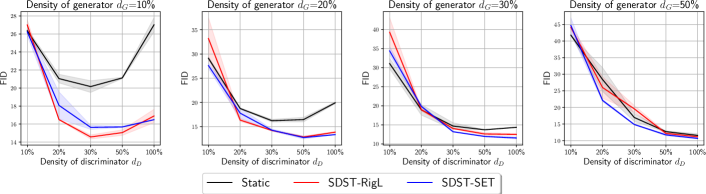
Figure 1: FID ($\downarrow$) comparison of SDST against STATIC sparse training for SNGAN on CIFAR-10 with different sparsity ratio combinations. The shaded areas denote the standard deviation.

To support our claim, we conduct experiments with SNGAN (Miyato et al., 2018) on the CIFAR-10 dataset. We consider the following sparse training algorithms:

➊ Static sparse training (STATIC). For STATIC, layer-wise sparsity ratio and masks $\bm{m}_{G},\bm{m}_{D}$ are fixed throughout the training.

➋ Single dynamic sparse training (SDST). SDST is a direct application of the DST method on GANs where only the generator dynamically adjusts masks during the training. We name such method SDST as only one component of the GAN, i.e., the generator, is dynamic. Furthermore, we call the variant which grows connections based on gradients magnitude as * ∘ SDST-RigL (Evci et al., 2020), and randomly as * ⋄ SDST-SET (Mocanu et al., 2018). Note that STU-GAN (Liu et al., 2022) is almost identical to * ∘ SDST-RigL with EMA (Yaz et al., 2018) tailored for DST. We do not consider naively applying DST on both generators and discriminators, as in STU-GAN, it is empirically shown that simply adjusting both components generates worse performance with more severe training instability.

We test the considered algorithms with $d_{G}\in\{10\%,20\%,30\%,50\%\}$ and $d_{D}\in\{10\%,20\%,30\%,$ $50\%,100\%\}$. More experiment details can be found at Appendix A and Appendix B.

4.1 Key observations

We report the results in Figure 1 and summarize our critical findings as follows:

➊ Observation 1: Neither strong nor weak sparse discriminators can provide satisfactory results. The phenomenon is most noticeable when $d_{G}=10\%$, where the FID initially decreases but then increases. The reasons may be as follows: (1) Overly weak discriminators may cause training collapse as they cannot provide useful information to the generator, resulting in a sudden increase in FID at the early stage of sparse GAN training. (2) Overly strong discriminators may not yield good FID results because they learn too quickly, not allowing the generator to keep up. Hence, to ensure a balanced training of GAN for sparse training methods, it is crucial to find an appropriate sparsity ratio for the discriminator.

➋ Observation 2: SDST is unable to give stable performance boost compared to the STATIC baseline. Another critical observation is that SDST is better than STATIC only when the discriminator is strong enough. More specifically, for all selected discriminator density ratios, SDST method is not better than STATIC when using a small discriminator density ($d_{D}=10\%$). On the contrary, for the cases where $d_{D}>d_{G}$, we generally see a significant performance boost brought by SDST.

5 Balance ratio: Towards quantifying the unbalance in sparse GAN training

5.1 Formulation of the balance ratio

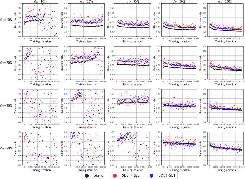
Figure 2: BR comparison of SDST against STATIC sparse training for SNGAN on CIFAR-10 with different sparsity ratio combinations.

To gain a deeper understanding of the phenomenon observed in the previous section, and to better monitor and control the degree of unbalance in sparse GANs, we introduce a novel quantity called the balance ratio (BR). This quantity is defined as follows.

At each training iteration, we draw random noise $\bm{z}$ from a multivariate normal distribution and real images $\bm{x}_{r}$ from the training set. We denote the discriminator after gradient descent update as $D(\cdot;\bm{\theta}_{D})$. We denote generator before and after gradient descent training as $G^{\text{pre}}(\cdot;\bm{\theta}_{G})$ and $G^{\text{post}}(\cdot;\bm{\theta}^{\prime}_{G})$, respectively. Then the balance ratio is defined as:

$$\text{BR}=\frac{\mathbb{E}_{\bm{z}\sim p}\left[D(G^{\text{post}}(\bm{z}))-D(G^{\text{pre}}(\bm{z}))\right]}{\mathbb{E}_{\bm{x}_{r}\sim p_{\text{data}}}[D(\bm{x}_{r})]-\mathbb{E}_{\bm{z}\sim p}[D(G^{\text{pre}}(\bm{z}))]}=\frac{\alpha}{\beta}.$$ (3)

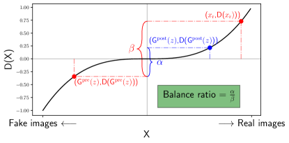
Figure 3: Illustration of balance ratio.

Precisely, BR measures how much improvement the generator can achieve in the scale measured by the discriminator for a specific random noise $\bm{z}$. When BR is too small (e.g., BR$<30\%$), the updated generator is too weak to trick the discriminator, as the generated images are still considered fake. Similarly, for the case where BR is too large (e.g., BR$>80\%$), the discriminator is considered too weak hence it may not provide useful information to the generator. We also illustrate BR in Figure 3.

5.2 Understanding observation 1: Analysing GAN balance with the balance ratio

We visualize the BR evolution throughout the training for the experiments in section 4 to show the effectiveness of BR in quantifying the balance of sparse GANs. We show the results in Figure 2.

It illustrates that BR can distinguish the density difference (hence the representation power difference) of the discriminator. Specifically, we can see that for larger discriminator density $d_{D}$, the BR is much lower throughout the training, indicating strong discriminators. On the contrary, for the cases where the discriminators are too weak compared to the generators, e.g., all cases where $d_{D}=10\%$, we can observe BR first increases and then oscillates wildly. We believe this oscillatory behavior is related to the training collapse. Empirical results also show that the FID metric experiences a sudden increase after this turning point.

5.3 Dynamic density adjust: A first attempt to utilize the balance ratio

As demonstrated in the previous section, the balance ratio (BR) effectively captures the degree of balance between the generators and discriminators in sparse GANs. Hence, it is natural to leverage BR to dynamically adjust the density of discriminators during sparse GAN training so that a reasonable discriminator density can be found.

To demonstrate the value of BR, we propose a simple yet powerful modification to the STATIC baseline. This method, which we call dynamic density adjust (DDA), is explained below. Specifically, we initialize the initial density of the discriminator $d^{\text{init}}_{D}=d_{G}$. After a specific training iteration interval, we adjust the density of the discriminator based on the BR over the last few iterations with a pre-defined density increment $\Delta d$. With a pre-defined BR bounds $[B_{-},B_{+}]$, we decrease $d_{D}$ by $\Delta d$ when BR is smaller than $B_{-}$, and vise versa. We show the algorithm in Appendix C Algorithm 1.

Comparison to ADA (Karras et al., 2020a). In this paragraph, we compare ADA and DDA. (1) Notice that DDA algorithm is orthogonal to ADA in a sense that StyleGAN2-ADA adjusts the data augmentation probability while DDA adjusts the discriminator density. (2) Moreover, the criterion used in DDA, i.e. BR, is very different from the criterion proposed in StyleGAN2-ADA, i.e. $r_{v}=\frac{\mathbb{E}\left[D(x_{\text{train}})\right]-\mathbb{E}\left[D(x_{\text{val}})\right]}{\mathbb{E}\left[D(x_{\text{train}})\right]-\mathbb{E}\left[D(G(z))\right]}$ and $r_{t}=\mathbb{E}\left[\text{sign}(D(x_{\text{train}}))\right]$. In particular, $r_{v}$ requires a separate validation set, while $r_{t}$ only quantifies the overfitting of the discriminator to the training set. (3) Another note is that DDA is a flexible framework, where its criterion, i.e. BR, can be potentially replaced by $r_{v}$, $r_{t}$, and such.

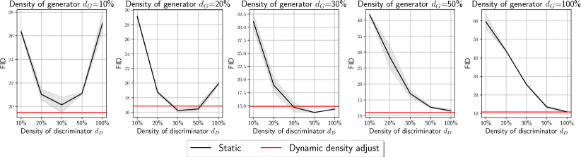
Figure 4: FID ($\downarrow$) of STATIC sparsely trained SNGAN with and without DDA on CIFAR-10 with different sparsity ratio combinations. The result of DDA is independent of $d_{D}$ as it is determined automatically. The shaded areas denote the standard deviation.

Experiment results. We test DDA with target BR interval $[B_{-},B_{+}]=[0.5,0.65]$. Precisely, DDA tends to find a suitable discriminator where the generator can just trick the discriminator throughout the training. We show the results in Figure 4 with red lines. The experiments show that DDA can identify reasonable discriminator densities to enable balanced training for sparse GANs.

5.4 Understanding observation 2: Analysing the failure of SDST with the balance ratio

By leveraging BR, we can also gain further insights into why some configurations do not benefit from SDST as compared to STATIC.

Regarding SDST as a way of increasing the generator capacity. Our findings suggest that SDST can possibly enhance the generator’s representation power, as demonstrated by the higher BR values compared to STATIC observed in Figure 2. We attribute this effect to the in-time over-parameterization (ITOP) (Liu et al., 2021c) induced by dynamic sparse training.

SDST does not address training collapse. The increase in generator’s representation power resulting from SDST is only beneficial when the discriminator has matching or superior representation power. Therefore, if the training has already collapsed for the static baseline methods (STATIC), meaning that the generator is already stronger than the discriminator, SDST may not be effective in stabilizing sparse GAN training. This is evident from the results shown in Figure 2 first-row column 1, second-row column 1, third-row columns 1-2, and fourth-row columns 1-3.

Despite the superior performance of STU-GAN (or SDST in general) at higher discriminator density ratios $d_{D}$, there exist some limitations for SDST, which we summarize below:

➊ SDST requires a pre-defined discriminator density $d_{D}$ before training. However, it is unclear what is a good choice. In real-world scenarios, it is not practical to manually search for the optimal $d_{D}$ for each $d_{G}$. A workaround may be using the maximum allowed density for the discriminator. However, as shown in Figure 1, the best performance is not always obtained with the maximum $d_{D}=100\%$. Moreover, we are wasting extra computational cost for a worse performance if we use an overly-strong discriminator.

➋ SDST fails if there is an additional constraint on the density of the discriminator $d_{D}$. As Figure 1 suggests, for weak discriminators, SDST is unable to show consistent improvement compared to the STATIC baseline.

Hence, STU-GAN (or SDST in general), which directly applies DST to the generator, may only be useful when the corresponding discriminator is strong enough. In this sense, obtaining balanced training automatically is essential in GAN DST to deal with more complicated scenarios.

6 Balanced dynamic sparse training for GANs

In this section, we describe our methodology for balanced sparse GAN training.

STU-GAN (or SDST in general) considered in the last section cannot generate stable and satisfying performance. This implies that we should utilize the discriminator in a better way rather than do nothing (like SDST) or directly apply DST to the discriminator (see subsection E.2 for additional experiments). Consequently, DDA (subsection 5.3), which adjusts the discriminator density to stabilize GAN training, is a favorable candidate to address the issue. To this end, we propose bAlanced DynAmic sParse Training (ADAPT), which adjusts the density of the discriminator during training with DDA while the generator performs DST.

We further introduce two variants, namely ADAPT${}_{\text{relax}}$ and ADAPT${}_{\text{strict}}$, based on whether we force the discriminator to be sparse. We present them in subsection 6.1 and subsection 6.2. These methods are more flexible and generate more stable performance compared to SDST.

6.1 ADAPT${}_{\text{relax}}$: Balanced dynamic sparse training in the relaxed setting

In this section, we consider the relaxed setting where a dense discriminator can be used, i.e., $d_{D}\leq d_{\text{max}}=100\%$. This relaxed scenario gives the greatest flexibility to the discriminator. However, it does not necessarily enforce the sparsity of the discriminator (hence, no computational savings for the discriminator) because the density of the discriminator can be as high as $100\%$.

For the relaxed setting, we use the direct combination of SDST with DDA. Precisely, the generator is adjusted using DST as mentioned in section 4 while the density of the discriminator is dynamically adjusted with DDA as mentioned in subsection 5.3. We call such a combination relaxed balanced dynamic sparse training (ADAPT${}_{\text{relax}}$). Please see Appendix C Algorithm 2 for more details.

Comparison to STU-GAN (or SDST in general). Compared to STU-GAN (or SDST in general), which pre-defines and fixes the discriminator density during training, the difference is that for ADAPT${}_{\text{relax}}$, the density of the discriminator is adjusted during the training process automatically through real-time monitoring of the balance ratio. Given the initial discriminator density $d_{D}^{\text{int}}=d_{G}$, ADAPT${}_{\text{relax}}$ increases the discriminator density if a stronger discriminator is needed, and vice versa.

6.2 ADAPT${}_{\text{strict}}$: Balanced dynamic sparse training in the strict setting

Different from subsection 6.1, we now consider a strict setting where there is an additional sparsity constraint on the discriminator density in this section, i.e., $d_{D}\leq d_{\text{max}}<100\%$.

ADAPT${}_{\text{relax}}$ introduced in the previous section does not necessarily enforce sparsity for the discriminator, which provides less memory/training resources saving for larger generator density ratios. Note that the discriminator does not take advantage of DST to explore the structure of the dense network. Hence, we further present strict balanced dynamic sparse training (ADAPT${}_{\text{strict}}$) in this section. This method allows the discriminator to perform DST in a controlled manner, which can lead to a better exploration of the dense network structure while maintaining the balance between the generator and the discriminator. We explain how ADAPT${}_{\text{strict}}$ differs from ADAPT${}_{\text{relax}}$ below:

➊ Capacity increase of the discriminator. The essential difference lies when the observed BR is higher than $B_{+}$, which means we need a stronger discriminator. In this case, if the discriminator density is lower than the constraint, i.e., $d_{D}<d_{\text{max}}$, ADAPT${}_{\text{strict}}$ will perform just like ADAPT${}_{\text{relax}}$ to increase the discriminator density. However, if the discriminator is already the maximum density, i.e., $d_{D}=d_{\text{max}}$, the discriminator will alternatively perform DST as a way of increasing the discriminator capacity (See subsection 5.4 for intuition).

➋ Capacity decrease of the discriminator. Similar to ADAPT${}_{\text{relax}}$, when the observed BR is lower than $B_{-}$, we will decrease the discriminator density.

Hence, ADAPT${}_{\text{strict}}$ makes the discriminator adaptive both in the density level (through density adjustment) and the parameter level (through DST). The algorithm of ADAPT${}_{\text{strict}}$ is shown in Appendix C Algorithm 3.

Table 1: FID ($\downarrow$) of different sparse training methods with no constraint on the density of the discriminator. Best results are in bold; second-best results are underlined.

Dataset	CIFAR-10 (SNGAN)				STL-10 (SNGAN)				CIFAR-10 (BigGAN)				TinyImageNet (BigGAN)
Generator density	10%	20%	30%	50%	10%	20%	30%	50%	10%	20%	30%	50%	10%	20%	30%	50%
(Dense Baseline)	10.74				29.71				8.11				15.43
STATIC-Balance	26.75	19.04	15.05	12.24	48.18	44.67	41.73	37.68	16.98	12.81	10.33	8.47	28.78	21.67	18.86	17.51
STATIC-Strong	26.79	19.65	14.38	11.91	52.48	43.85	42.06	37.47	23.48	14.26	11.19	8.64	31.44	22.51	18.22	18.00
* ⋄ SDST-Balance-SET	26.23	17.79	13.21	11.79	56.41	46.58	39.93	30.37	12.41	9.87	9.13	8.01	25.39	21.30	21.80	21.20
* ⋄ SDST-Strong-SET	16.49	13.36	11.68	10.68	67.37	49.96	37.99	31.08	18.94	9.64	8.75	8.36	22.20	20.56	21.70	18.32
* ∘ SDST-Balance-RigL	27.06	16.36	14.00	12.28	43.08	33.90	31.83	30.30	12.45	9.42	8.86	8.03	21.60	19.33	18.57	17.45
* ∘ SDST-Strong-RigL	17.02	13.86	12.51	11.35	53.65	33.25	31.41	30.18	10.58	9.11	8.69	8.33	21.14	18.95	17.75	16.30
$\text{ADAPT}_{\text{relax}}$ (Ours)	14.19	13.19	12.38	10.60	35.98	33.06	31.71	29.96	10.19	8.56	8.36	8.22	19.42	17.99	17.06	14.15

Table 2: FID ($\downarrow$) of different sparse training methods. The density of the discriminator is constrained to be lower than 50%. Best results are in bold; second-best results are underlined.

Dataset	CIFAR-10 (SNGAN)				STL-10 (SNGAN)				CIFAR-10 (BigGAN)				TinyImageNet (BigGAN)
Generator density	10%	20%	30%	50%	10%	20%	30%	50%	10%	20%	30%	50%	10%	20%	30%	50%
(Dense Baseline)	10.74				29.71				8.11				15.43
STATIC-Balance	26.75	19.04	15.05	12.58	48.18	44.67	41.73	37.68	16.98	12.81	10.33	8.47	28.78	21.67	18.86	17.51
STATIC-Strong	21.73	16.69	13.48	12.58	50.36	44.06	40.73	37.68	18.91	13.43	10.84	8.47	33.01	23.93	17.90	17.51
* ⋄ SDST-Balance-SET	26.23	17.79	13.21	11.79	56.24	44.51	41.23	30.80	12.41	9.87	9.13	8.01	25.39	21.30	21.80	21.20
* ⋄ SDST-Strong-SET	15.68	12.75	11.98	11.79	57.91	50.05	38.13	30.80	11.85	9.39	8.61	8.01	22.68	20.24	22.00	21.20
* ∘ SDST-Balance-RigL	27.06	16.36	14.00	12.28	43.08	33.90	31.64	30.30	12.45	9.42	8.86	8.03	21.60	19.33	18.57	17.45
* ∘ SDST-Strong-RigL	15.19	12.93	12.75	12.28	53.74	37.34	31.98	30.30	10.11	9.17	8.35	8.03	21.90	20.43	18.29	17.45
$\text{ADAPT}_{\text{strict}}$ (Ours)	14.53	12.73	12.20	12.11	41.18	31.59	31.16	29.11	9.29	8.64	8.44	7.90	18.89	17.37	16.93	16.02

6.3 Experiment setting

Datasets, architectures, and target sparsity ratios. We conduct experiments on SNGAN with ResNet architectures on the CIFAR-10 and the STL-10 (Coates et al., 2011) datasets. We have also conducted experiments with BigGAN (Brock et al., 2018) on the CIFAR-10 and TinyImageNet dataset (with DiffAug (Zhao et al., 2020)). Target density ratios of the generators $d_{G}$ are chosen from $\{10\%,20\%,30\%,50\%\}$. Please see Appendix A for more experiment details.

Baseline methods and two practical strategies. We use STATIC and SDST (section 4) as our baselines. Note that in real-world application scenarios, it is not practical to perform a grid search for a good $d_{D}$ as in section 4. Hence, we propose two practical strategies to define the constant discriminator density for these baseline methods: (1) balance strategy, where we set the density of the discriminator $d_{D}$ the same as the density of the generator $d_{G}$; (2) strong strategy, where we set the density of the discriminator as large as possible, i.e., $d_{D}=d_{\text{max}}$. For SDST methods, we test both * ⋄ SDST-SET and * ∘ SDST-RigL. For a fair comparison, $d_{\text{max}}$ is set to be 100% and 50% for the relaxed setting and the strict setting, respectively.

For ADAPT${}_{\text{,}}$ we use the * ∘ RigL version, which grows connections of the generators and discriminators based on gradient magnitude. The gradient information enables two components to react promptly according to the change of each other. Different from the value used in subsection 5.3, we control the balance ratio in the range $\left[0.45,0.55\right]$ unless otherwise mentioned to have a slightly stronger discriminator, potentially avoiding training collapse. More details can be found in Appendix B.

6.4 Experiment results

Table 3: Normalized training FLOPs ($\downarrow$) of different sparse training methods with no constraint on the density of the discriminator.

Dataset	CIFAR-10 (SNGAN)				STL-10 (SNGAN)				CIFAR-10 (BigGAN)				TinyImageNet (BigGAN)
Generator density	10%	20%	30%	50%	10%	20%	30%	50%	10%	20%	30%	50%	10%	20%	30%	50%
(Dense Baseline)	100% ($2.67\times 10^{17}$)				100% ($3.94\times 10^{17}$)				100% ($6.81\times 10^{17}$)				100% ($9.85\times 10^{17}$)
Static-Balance	8.97%	17.08%	26.25%	47.25%	27.30%	47.14%	59.22%	73.35%	9.79%	19.02%	28.66%	49.03%	23.25%	44.87%	60.91%	79.29%
Static-Strong	58.29%	60.94%	64.53%	74.61%	86.12%	86.94%	87.60%	88.84%	83.78%	84.80%	86.21%	90.15%	48.02%	61.62%	72.79%	85.79%
* ⋄ SDST-Balance-SET	9.78%	18.91%	28.35%	48.44%	27.55%	47.60%	60.17%	75.38%	10.35%	20.12%	29.96%	49.82%	21.13%	37.06%	48.83%	65.58%
* ⋄ SDST-Strong-SET	59.25%	62.94%	66.89%	75.96%	86.36%	87.43%	88.49%	90.82%	84.36%	85.90%	87.52%	90.95%	45.66%	53.91%	60.61%	71.88%
* ∘ SDST-Balance-RigL	10.71%	17.43%	25.66%	43.56%	29.51%	50.41%	63.34%	79.03%	9.92%	19.30%	28.90%	48.31%	24.97%	43.86%	57.26%	76.75%
* ∘ SDST-Strong-RigL	58.63%	61.35%	64.04%	71.01%	88.51%	90.24%	91.78%	94.57%	83.97%	85.24%	86.59%	89.54%	50.05%	61.02%	69.64%	83.35%
$\text{ADAPT}_{\text{relax}}$ (Ours)	36.67%	57.62%	61.31%	70.11%	46.73%	77.92%	83.62%	90.49%	10.39%	25.90%	40.65%	80.76%	29.75%	51.98%	64.57%	80.81%

We show the experiment results in Table 1 and Table 2 for the relaxed setting and the strict setting, respectively. We also present the training FLOPs normalized by the dense counterpart for the relaxed setting in Table 3. We defer the results for the strict setting to Appendix F Table 12. We show FID for the CIFAR-10 test set, Inception scores, and comparison with post-hoc pruning baseline in Appendix E. We also show ADAPT BR evolution in Appendix D. We summarize our findings below.

The strong strategy and the balance strategy for baselines. Generally, using the strong strategy has some advantages over the balance strategy. Such an observation is most prominent in the CIFAR-10 dataset. For the cases where the balance strategy is better, e.g., SNGAN on the STL-10 dataset, our explanation is that the size difference between generators and discriminators is more significant. Hence, the degree of unbalance is more severe and leads to more detrimental effects.

Comparison of * ∘ RigL and * ⋄ SET for SDST. We found that * ∘ RigL has an advantage over * ⋄ SET when dealing with more sparse generators. Our hypothesis is that gradient information can effectively guide the generator to identify the most crucial connections in such cases. However, this advantage is not as apparent for more dense generators.

ADAPT${}_{\text{relax}}$ achieves a good trade-off between performance and computational cost. Experiments show that ADAPT${}_{\text{relax}}$ shows promising performance by being best for 13 out of 16 cases. The advantage of ADAPT${}_{\text{relax}}$ is most prominent for the most difficult case, i.e., $d_{G}=10\%$. Specifically, it shows 2.3 and 7.1 FID improvements over the second-best methods for the SNGAN on the CIFAR-10 and the STL-10, respectively. Moreover, compared to the competitive baseline methods that use the strong strategy, i.e., * ∘ SDST-Strong-RigL and * ⋄ SDST-Strong-SET, ADAPT${}_{\text{relax}}$ shows great computational cost reduction. For example, it outperforms * ∘ SDST-Strong-RigL on BigGAN (CIFAR-10) with much-reduced training FLOPs (10.39% v.s. 83.97%).

ADAPT${}_{\text{strict}}$ shows stable and superior performance. Similar to ADAPT${}_{\text{relax}}$, we notice that ADAPT${}_{\text{strict}}$ also delivers promising results compared to baselines, even with a further constraint on the discriminator. More precisely, among all the cases, ADAPT${}_{\text{strict}}$ ranks top 2 for all cases, with 13 cases being the best. Moreover, ADAPT${}_{\text{strict}}$ again shows comparable or better performance compared to * ∘ SDST-Strong-RigL with reduced computational cost.

A more interesting observation is that ADAPT${}_{\text{strict}}$ sometimes outperforms ADAPT${}_{\text{relax}}$. We speculate that this phenomenon occurs because changes in density may result in a larger influence on the GAN balance during training compared to DST. Hence, the strict version, whose discriminator density range is smaller, may offer a more consistent performance.

7 Conclusion

In this paper, we investigate the use of DST for GANs and find that solely applying DST to the generator does not necessarily enhance the performance of sparse GANs. To address this, we introduce BR to examine the degree of unbalance between the sparse generators and discriminators. We find that applying DST to the generator only benefits the training when the discriminator is comparatively stronger. Additionally, we propose ADAPT, which can dynamically adjust the discriminator at both the parameter and density levels. Our approach shows promising results, and we hope it can aid researchers in better comprehending the interplay between the two components of GAN training and motivate further exploration of sparse training for GANs. However, we must note that we have not yet evaluated our methods on the latest GAN architectures due to computational constraints.

8 Acknowledgement

This work utilizes resources supported by the National Science Foundation’s Major Research Instrumentation program, grant No.1725729 (Kindratenko et al., 2020), as well as the University of Illinois at Urbana-Champaign. This work is supported in part by Hetao Shenzhen-Hong Kong Science and Technology Innovation Cooperation Zone Project (No.HZQSWS-KCCYB-2022046); University Development Fund UDF01001491 from the Chinese University of Hong Kong, Shenzhen; Guangdong Key Lab on the Mathematical Foundation of Artificial Intelligence, Department of Science and Technology of Guangdong Province. Prof. NH is in part supported by Air Force Office of Scientific Research (AFOSR) grant FA9550-21-1-0411.

Overview of the Appendix

The Appendix is organized as follows:

• Appendix A introduces the general experimental setup.

• Appendix B introduces the details of dynamic sparse training.

• Appendix C shows detailed algorithms, i.e., DDA, ADAPT${}_{\text{relax}}$, and ADAPT${}_{\text{strict}}$.

• Appendix D shows the BR evolution during training for ADAPT.

• Appendix E shows additional results, including IS and FID of test sets of the main paper.

• Appendix F shows detailed FLOPs comparisons of sparse training methods.

Appendix A Experimental setup

In this section, we explain the training details used in our experiments. Our code is mainly based on the original code of ITOP [Liu et al., 2021c] and GAN ticket [Chen et al., 2021b].

A.1 Architecture details

We use ResNet-32 [He et al., 2016] for the CIFAR-10 dataset and ResNet-48 for the STL-10 dataset. See Table 5 and Table 5 for detailed architectures. We apply spectral normalization for all fully-connected layers and convolutional layers of the discriminators.

For BigGAN architecture, we use the implementation used in DiffAugment [Zhao et al., 2020].

A.2 Datasets

We use the training set of CIFAR-10, the unlabeled partition of STL-10, and the training set of TinyImageNet for GAN training. Training images are resized to $32\times 32$, $48\times 48$, $64\times 64$ for CIFAR-10, STL-10, and TinyImageNet datasets, respectively. Augmentation methods for both datasets are random horizontal flip and per-channel normalization.

A.3 Training hyperparameters

SNGAN on the CIFAR-10 and STL-10 datasets. We use a learning rate of $2\times 10^{-4}$ for both generators and discriminators. The discriminator is updated five times for every generator update. We adopt Adam optimizer with $\beta_{1}=0$ and $\beta_{2}=0.9$. The batch size of the discriminator and the generator is set to 64 and 128, respectively. Hinge loss is used following [Brock et al., 2018, Chen et al., 2021b]. We use exponential moving average (EMA) [Yaz et al., 2018] with $\beta=0.999$. The generator is trained for a total of 100k iterations.

BigGAN on the CIFAR-10 dataset. We use a learning rate of $2\times 10^{-4}$ for both generators and discriminators. The discriminator is updated four times for every generator update. We adopt Adam optimizer with $\beta_{1}=0$ and $\beta_{2}=0.999$. The batch size of both the discriminator and the generator is set to 50. Hinge loss is used following [Brock et al., 2018, Wu et al., 2021]. We use EMA with $\beta=0.9999$. The generator is trained for a total of 200k iterations.

BigGAN on the TinyImageNet dataset. We use DiffAug [Zhao et al., 2020] to augment the input. The learning rate of the discriminator and the generator are set to $4\times 10^{-4}$ and $1\times 10^{-4}$, respectively. The discriminator is updated one time for every generator update. We adopt Adam optimizer with $\beta_{1}=0$ and $\beta_{2}=0.999$. The batch size of both the discriminator and the generator is set to 256. Hinge loss is used following [Brock et al., 2018, Wu et al., 2021]. We use EMA with $\beta=0.9999$. The generator is trained for a total of 200k iterations.

A.4 Evaluation metric

SNGAN on the CIFAR-10 and the STL-10 datasets. We compute Fréchet inception distance (FID) and Inception score (IS) for 50k generated images every 5000 iterations. Best FID and IS are reported. For the CIFAR-10 dataset, we report both FID for the training set and test set, whereas, for the STL-10 dataset, we report the FID of the unlabeled partition.

BigGAN on the CIFAR-10 and the TinyImageNet dataset. We compute Fréchet inception distance (FID) and Inception score (IS) for 10k generated images every 5000 iterations. Best FID and IS are reported.

Appendix B Dynamic sparse training details

B.1 How the generator performs DST

In this section, we explain how the generator performs DST below. Note that the generator performs the same for SDST and ADAPT.

Sparsity distribution at initialization. Following RigL and ITOP [Evci et al., 2020, Liu et al., 2021c], only parameters of fully connected and convolutional layers will be pruned. At initialization, we use the commonly adopted Erdős-Rényi-Kernel (ERK) strategy [Evci et al., 2020, Dettmers and Zettlemoyer, 2019, Liu et al., 2021c] to allocate higher sparsity to larger layers. Specifically, the sparsity of convolutional layers $l$ is scaled with $1-\frac{n^{l-1}+n^{l}+w^{l}+h^{l}}{n^{l-1}n^{l}w^{l}h^{l}}$, where $n^{l}$ denotes the number of channels of layer $l$ while $w^{l}$ and $h^{l}$ are the widths and the height of the corresponding kernel in that layer. For fully connected layers, Erdős-Rényi (ER) strategy is used, where the sparsity is scaled with $1-\frac{n^{l-1}+n^{l}}{n^{l-1}n^{l}}$.

Update schedule. The update schedule controls how many connections are adjusted per DST operation. It can be specified by the number of training iterations between sparse connectivity updates $\Delta T_{G}$, the initial fraction of connections adjusted ${\gamma}$, and decaying schedule $f_{\text{decay}}({\gamma},T)$ for ${\gamma}$.

Drop and grow. After $\Delta T_{G}$ training iterations, we update the mask $\bm{m}_{G}$ by dropping/pruning $f_{\text{decay}}({\gamma},T)\left|\bm{\theta}_{G}\right|d_{G}$ number of connections with the lowest magnitude, where $\left|\bm{\theta}_{G}\right|$, $d_{G}$ are the number of parameters and target density for the generator, $f_{\text{decay}}({\gamma},T)$ is the update schedule. Right after the connection drop, we regrow the same amount of connections.

For the growing criterion, we test both random growth * ⋄ SET [Mocanu et al., 2018, Liu et al., 2021c] and gradient-based growth * ∘ RigL [Evci et al., 2020]. Concretely, gradient-based methods find newly-activated connections $\theta$ with the highest gradient magnitude $\left|\frac{\partial\mathcal{L}}{\partial\theta}\right|$, while random-based methods explore connections in a random fashion. All the newly-activated connections are set to 0. One thing that should be noticed is that while previous works consider layer-wise connections drop and growth, we grow and drop connections globally as it grants more flexibility to the DST method.

EMA for sparse GAN. EMA [Yaz et al., 2018] is well-known for its ability to alleviate the non-convergence of GAN. We also implement EMA for sparse GAN training. Specifically, we zero out the moving average of dropped weights whenever there is a mask change.

B.2 DST hyperparameters for the generator

We use the same hyper-parameters for SDST and ADAPT. The initial $\gamma$ is set to 0.5, and we use a cosine annealing function $f_{\text{decay}}$ following RigL and ITOP.

SNGAN on the CIFAR-10 and the STL-10 datasets. The connection update frequency of the generator $\Delta T_{G}$ is set to 500 and 1000 for the CIFAR-10 dataset and STL-10 dataset, respectively.

BigGAN on the CIFAR-10 and the TinyImageNet dataset. The connection update frequency of the generator $\Delta T_{G}$ is set to be 1000.

B.3 Density dynamic adjust (DDA) hyper-parameters

In this section, we provide hyper-parameters used in subsection 5.3. We set $d_{D}=2000$ , $\Delta T_{D}=0.05$, $\left[B_{-},B_{+}\right]=[0.5,0.65]$. Time-averaged BR over 1000 iterations is used as the indicator.

B.4 DST hyperparameters for the discriminator in ADAPT

We use a constant BR interval $[B_{-},B_{+}]=[0.45,0.55]$ for SNGAN experiments and BigGAN on the CIFAR-10 dataset. We set the BR interval $[B_{-},B_{+}]=[0.3,0.4]$ for BigGAN on the TinyImageNet since it uses DiffAug. Time-averaged BR over 1000 iterations is used as the indicator. Density increment $\Delta d$ is set to be 0.05, 0.025, and 0.05 for SNGAN (CIFAR-10), SNGAN (STL-10), and BigGAN (CIFAR-10), respectively. We use the same setting used in subsection B.2 for the generator.

Hyper-parameters for ADAPT${}_{\text{relax}}$. The density update frequency of the discriminator $\Delta T_{D}$ is 1000, 2000, 5000, and 10000 iterations for SNGAN (CIFAR-10), SNGAN (STL-10), BigGAN (CIFAR-10), and BigGAN (TinyImageNet), respectively.

Hyper-parameters for ADAPT${}_{\text{strict}}$. The density/connections update frequency of the discriminator $\Delta T_{D}$ is 2000, 2000, 5000, and 10000 iterations for SNGAN (CIFAR-10), SNGAN (STL-10), BigGAN (CIFAR-10), and BigGAN (TinyImageNet), respectively.

Note that we compute BR for every iteration to visualize the BR evolution, whereas one should note that such computational cost can be greatly decreased if BR is computed every few iterations.

Table 4: ResNet architecture for CIFAR-10.

(a) Generator	(b) Discriminator
$z\in\mathbb{R}^{128}\sim\mathcal{N}(0,I)$	image $x\in[-1,1]^{32\times 32\times 3}$
dense, $4\times 4\times 256$	ResBlock down 128
ResBlock up 256	ResBlock down 128
ResBlock up 256	ResBlock down 128
ResBlock up 256	ResBlock down 128
BN, ReLU, $3\times 3$ conv, Tanh	ReLU 0.1
	Global sum pooling
	dense $\rightarrow$ 1

Table 5: ResNet architecture for STL-10.

(a) Generator	(b) Discriminator
$z\in\mathbb{R}^{128}\sim\mathcal{N}(0,I)$	image $x\in[-1,1]^{48\times 48\times 3}$
dense, $6\times 6\times 512$	ResBlock down 64
ResBlock up 256	ResBlock down 128
ResBlock up 128	ResBlock down 256
ResBlock up 64	ResBlock down 512
BN, ReLU, $3\times 3$ conv, Tanh	ResBlock down 1024
	ReLU 0.1
	Global avg pooling
	dense $\rightarrow$ 1

Appendix C Algorithms

In this section, we present the detailed algorithms for DDA, ADAPT${}_{\text{relax}}$, and ADAPT${}_{\text{strict}}$.

C.1 Dynamic adjust algorithm

We first present DDA in Algorithm 1.

Algorithm 1 Dynamic density adjust (DDA) for the discriminator.

0:  Generator $G$, discriminator $D$, BR upper bound $B_{+}$ and lower bound $B_{-}$, DA interval $\Delta T_{D}$, density increment $\Delta d$, current training iteration $t$.

1:  if $t\mod\Delta T_{D}==0$ then

2:     Compute time-averaged BR with Equation 3

3:     if $\text{BR}>B_{+}$ then

4:        Increase the density of discriminator from $d_{D}$ to $d_{D}+\Delta d$.

5:     else if $\text{BR}<B_{-}$ then

6:        Decrease the density of discriminator from $d_{D}$ to $d_{D}-\Delta d$.

7:     end if

8:  end if

Algorithm 2 Relaxed balanced dynamic sparse training (ADAPT${}_{\text{relax}}$) for GANs.

0:  Generator $G$, discriminator $D$, total number of training iterations $T$, number of training steps for discriminator in each iteration $N$, discriminator adjustment interval $\Delta T_{D}$, DST interval for the generator $\Delta T_{G}$, density increment $\Delta d$, target generator density $d_{G}$, BR upper bound $B_{+}$ and lower bound $B_{-}$.

1:  Set initial discriminator density $d_{D}=d_{G}$

2:  for $t$ in $\left[1,\cdots,T\right]$ do

3:     for $n$ in $\left[1,\cdots,N\right]$ do

4:        Compute the loss of discriminator $\mathcal{L}_{D}(\bm{\theta}_{D})$

5:        $\mathcal{L}_{D}(\bm{\theta}_{D}).backward()$

6:     end for

7:     if $t\mod\Delta T_{D}==0$ then

8:        Compute the loss of generator $\mathcal{L}_{G}(\bm{\theta}_{G})$

9:        $\mathcal{L}_{G}(\bm{\theta}_{G}).backward()$

10:        Compute time-averaged BR with Equation 3

11:        if  $\text{BR}>B_{+}$ then

12:           Increase the density of discriminator from $d_{D}$ to $\min(100\%,d_{D}+\Delta d)$.

13:        else if $\text{BR}<B_{-}$ then

14:           Decrease the density of discriminator from $d_{D}$ to $\max(0\%,d_{D}-\Delta d)$.

15:        end if

16:     end if

17:     if $t\mod\Delta T_{G}==0$ then

18:        Apply DST to $G$

19:     end if

20:  end for

C.2 Relaxed balanced dynamic sparse training algorithm

Details of ADAPT${}_{\text{relax}}$ algorithm is presented in Algorithm 2.

C.3 Strict balanced dynamic sparse training algorithm

Details of ADAPT${}_{\text{strict}}$ algorithm is presented in Algorithm 3.

Algorithm 3 Strict balanced dynamic sparse training (ADAPT${}_{\text{strict}}$) for GANs.

0:  Generator $G$, discriminator $D$, total number of training iterations $T$, number of training steps for discriminator in each iteration $N$, given maximal density of discriminator $d_{\text{max}}$, discriminator adjustment interval $\Delta T_{D}$, DST interval for the generator $\Delta T_{G}$, density increment $\Delta d$, target generator density $d_{G}$, BR upper bound $B_{+}$ and lower bound $B_{-}$.

1:  Set initial discriminator density $d_{D}=d_{G}$

2:  for $t$ in $\left[1,\cdots,T\right]$ do

3:     for $n$ in $\left[1,\cdots,N\right]$ do

4:        Compute the loss of discriminator $\mathcal{L}_{D}(\bm{\theta}_{D})$

5:        $\mathcal{L}_{D}(\bm{\theta}_{D}).backward()$

6:     end for

7:     if $t\mod\Delta T_{D}==0$ then

8:        Compute the loss of generator $\mathcal{L}_{G}(\bm{\theta}_{G})$

9:        $\mathcal{L}_{G}(\bm{\theta}_{G}).backward()$

10:        Compute time-averaged BR with Equation 3

11:        if  $\text{BR}>B_{+}$ and $d_{D}<d_{\text{max}}$ then

12:           Increase the density of discriminator from $d_{D}$ to $\min(d_{\text{max}},d_{D}+\Delta d)$.

13:        else if $\text{BR}>B_{+}$ and $d_{D}==d_{\text{max}}$ then

14:           Apply DST to $D$

15:        else if $\text{BR}<B_{-}$ then

16:           Decrease the density of discriminator from $d_{D}$ to $\max(0\%,d_{D}-\Delta d)$.

17:        end if

18:     end if

19:     if $t\mod\Delta T_{G}==0$ then

20:        Apply DST to $G$

21:     end if

22:  end for

Appendix D ADAPT balance ratio evolution

In this section, we show that ADAPT methods are able to maintain a BR throughout training. We show the time evolution of BR and discriminator density for BigGAN on the CIFAR-10 dataset.

Figure 5: Balance ratio and discriminator density evolution during training for ADAPT${}_{\text{relax}}$ on BigGAN (CIFAR-10). Dashed lines represent BR values of 0.45 and 0.55.

Results of ADAPT${}_{\text{relax}}$ and ADAPT${}_{\text{strict}}$ are shown in Figure 5 and Figure 6. It clearly illustrates the ability of ADAPT to keep the BR controlled during GAN training.

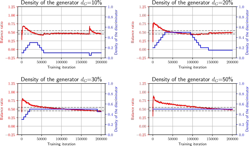
Figure 6: Balance ratio and discriminator density evolution during training for ADAPT${}_{\text{strict}}$ on BigGAN (CIFAR-10). Dashed lines represent BR values of 0.45 and 0.55.

Appendix E More experiment results

E.1 IS and FID for the CIFAR-10 dataset

In this section, we present corresponding IS scores results for Table 1 and Table 2. The results are shown in Table 9 and Table 9, respectively. We also include FID results of CIFAR-10 test set in Table 10.

E.2 Naively applying DST to both the generator and the discriminator

In this section, we follow STU-GAN to compare the baseline where applying DST on both generators and discriminators. We name it DST-bothGD.

We test on SNGAN (CIFAR-10) with $\Delta T_{D}=1000$, $\Delta T_{G}=500$, and $\gamma=0.5$. Note that we use the balance strategy where $d_{G}=d_{D}$. The reason is that the strong strategy uses a dense discriminator, and it does not make sense to apply DST to a dense network.

We show the results in Table 7. It shows that it generates unstable results and consistenly performs worse than SDST-Strong. So we do not compare such baseline in the main body of the paper.

E.3 Post-hoc pruning baseline

In this section, we compare different sparse training methods with post-hoc magnitude pruning [Renda et al., 2020] baseline. Magnitude pruning involves first training a dense generator, then pruning its weights globally based on their magnitudes. The pruned generator is then fine-tuned with the dense discriminator. We perform additional fine-tuning for $50\%$ of the original total iterations. Results are presented in Table 6.

Our experimental results clearly demonstrate the advantages of dynamic sparse training over post-hoc magnitude pruning. The latter typically requires around 150% normalized training FLOPs, while DST methods constantly achieve comparable or better performance with significantly reduced computational cost.

Table 6: FID ($\downarrow$) of different sparse training methods along with post-hoc pruning baseline with no constraint on the density of the discriminator. Best results are in bold; second-best results are underlined.

Dataset	CIFAR-10 (SNGAN)				STL-10 (SNGAN)				CIFAR-10 (BigGAN)
Generator density	10%	20%	30%	50%	10%	20%	30%	50%	10%	20%	30%	50%
(Dense Baseline)	10.74				29.71				8.11
Post-hoc pruning	20.89	14.07	12.99	11.90	57.28	37.12	31.98	29.70	15.44	10.84	9.65	8.77
STATIC-Balance	26.75	19.04	15.05	12.24	48.18	44.67	41.73	37.68	16.98	12.81	10.33	8.47
STATIC-Strong	26.79	19.65	14.38	11.91	52.48	43.85	42.06	37.47	23.48	14.26	11.19	8.64
* ⋄ SDST-Balance-SET	26.23	17.79	13.21	11.79	56.41	46.58	39.93	30.37	12.41	9.87	9.13	8.01
* ⋄ SDST-Strong-SET	16.49	13.36	11.68	10.68	67.37	49.96	37.99	31.08	18.94	9.64	8.75	8.36
* ∘ SDST-Balance-RigL	27.06	16.36	14.00	12.28	43.08	33.90	31.83	30.30	12.45	9.42	8.86	8.03
* ∘ SDST-Strong-RigL	17.02	13.86	12.51	11.35	53.65	33.25	31.41	30.18	10.58	9.11	8.69	8.33
$\text{ADAPT}_{\text{relax}}$ (Ours)	14.19	13.19	12.38	10.60	35.98	33.06	31.71	29.96	10.19	8.56	8.36	8.22

Table 7: FID ($\downarrow$) of different sparse training methods on CIFAR-10 datasets with no constraint on the density of the discriminator. Best results are in bold; second-best results are underlined.

Dataset	CIFAR-10
Generator density	10%	20 %	30 %	50 %
(Dense Baseline)	10.74
Static-Balance	26.75	19.04	15.05	12.24
Static-Strong	26.79	19.65	14.38	11.91
* ⋄ DST-bothGD-SET	20.57	14.90	12.58	11.86
* ∘ DST-bothGD-RigL	31.95	17.99	13.24	12.47
* ⋄ SDST-Balance-SET	26.23	17.79	13.21	11.79
* ⋄ SDST-Strong-SET	16.49	13.36	11.68	10.68
* ∘ SDST-Balance-RigL	27.06	16.36	14.00	12.28
* ∘ SDST-Strong-RigL	17.02	13.86	12.51	11.35
$\text{ADAPT}_{\text{relax}}$ (Ours)	14.19	13.19	12.38	10.60

Table 8: IS (higher is better) of different sparse training methods. There is no constraint on the density of the discriminator, i.e., $d_{\text{max}}=100\%$.

Dataset	SNGAN(CIFAR-10)				SNGAN(STL-10)				BigGAN(CIFAR-10)				BigGAN(TinyImageNet)
Generator density	10%	20 %	30 %	50 %	10%	20 %	30 %	50 %	10%	20 %	30 %	50 %	10%	20 %	30 %	50 %
(Dense Baseline)	8.48				9.16				8.99				14.65
Static-Balance	7.24	7.83	8.06	8.38	7.94	8.19	8.44	8.69	7.99	8.24	8.68	8.90	10.65	12.28	13.41	13.57
Static-Strong	7.52	8.03	8.32	8.45	7.70	8.22	8.35	8.70	7.75	8.13	8.52	8.99	10.45	12.56	13.61	13.73
* ⋄ SDST-Balance-SET	7.28	7.89	8.22	8.38	8.43	8.92	9.26	9.31	8.62	8.67	8.82	8.98	11.75	12.60	12.30	12.21
* ⋄ SDST-Strong-SET	8.37	8.54	8.57	8.60	7.65	8.53	9.39	9.21	8.16	8.78	8.85	9.06	12.75	12.84	12.46	13.73
* ∘ SDST-Balance-RigL	7.19	7.94	8.18	8.34	8.98	9.07	9.12	9.28	8.64	8.71	8.91	8.93	12.67	13.32	13.18	13.61
* ∘ SDST-Strong-RigL	8.32	8.52	8.59	8.57	8.15	9.10	9.16	9.17	8.65	8.72	8.97	9.00	13.32	13.35	13.60	14.47
ADAPT${}_{\text{relax}}$ (Ours)	8.42	8.44	8.54	8.60	9.08	9.29	9.06	9.26	8.74	9.07	8.98	9.00	13.09	13.57	13.68	15.77

Table 9: IS (higher is better) of different sparse training methods. The density of the discriminator is constrained to be lower than $d_{\text{max}}=50\%$.

Dataset	SNGAN(CIFAR-10)				SNGAN(STL-10)				BigGAN(CIFAR-10)				BigGAN(TinyImageNet)
Generator density	10%	20 %	30 %	50 %	10%	20 %	30 %	50 %	10%	20 %	30 %	50 %	10%	20 %	30 %	50 %
(Dense Baseline)	8.48				9.16				8.99				14.65
Static-Balance	7.24	7.83	8.06	8.38	7.94	8.19	8.44	8.69	7.99	8.24	8.68	8.90	10.65	12.28	13.41	13.57
Static-Strong	7.85	8.14	8.31	8.38	7.89	8.22	8.38	8.69	7.75	8.03	8.52	8.90	9.99	11.61	13.77	13.57
* ⋄ SDST-Balance-SET	7.28	7.89	8.22	8.38	8.43	8.92	9.26	9.31	8.62	8.67	8.82	8.98	11.75	12.60	12.30	12.21
* ⋄ SDST-Strong-SET	8.33	8.53	8.40	8.38	8.50	8.77	9.46	9.26	8.55	8.77	8.84	8.98	12.00	12.87	12.16	12.21
* ∘ SDST-Balance-RigL	7.19	7.94	8.18	8.34	8.98	9.07	9.12	9.28	8.64	8.71	8.91	8.93	12.67	13.32	13.18	13.61
* ∘ SDST-Strong-RigL	8.24	8.48	8.37	8.34	8.28	9.05	9.11	9.28	8.61	8.83	8.84	8.93	12.04	12.66	13.57	13.61
ADAPT${}_{\text{strict}}$ (Ours)	8.27	8.36	8.48	8.47	8.98	9.17	9.20	9.19	8.90	8.89	8.92	9.10	13.85	13.61	14.05	14.40

Table 10: FID of test set ($\downarrow$) of different sparse training methods on SNGAN (CIFAR-10) dataset. Best results are in bold; second-best results are underlined.

Maximal discriminator density $d_{\text{max}}$	100 %				50 %
Generator density	10%	20 %	30 %	50 %	10%	20 %	30 %	50 %
(Dense Baseline)	13.32
Static-Balance	29.56	21.79	17.80	14.94	29.56	21.79	17.80	14.94
Static-Strong	29.50	22.45	17.12	14.58	24.62	19.43	16.32	14.94
* ⋄ SDST-Balance-SET	28.84	20.31	15.95	14.35	28.84	20.31	15.95	14.35
* ⋄ SDST-Strong-SET	19.16	16.12	14.45	13.50	18.38	15.33	14.78	14.35
* ∘ SDST-Balance-RigL	29.77	19.02	16.68	15.05	29.77	19.02	16.68	15.05
* ∘ SDST-Strong-RigL	19.72	16.50	15.20	14.09	17.92	15.51	15.52	15.05
ADAPT${}_{\text{relax}}$ (Ours)	16.82	15.85	15.14	13.37	-	-	-	-
ADAPT${}_{\text{strict}}$ (Ours)	-	-	-	-	17.19	15.57	14.92	14.80

Table 11: FID of test set ($\downarrow$) of different sparse training methods on BigGAN (CIFAR-10) dataset. Best results are in bold; second-best results are underlined.

Maximal discriminator density $d_{\text{max}}$	100 %				50 %
Generator density	10%	20 %	30 %	50 %	10%	20 %	30 %	50 %
(Dense Baseline)	10.36
Static-Balance	19.58	15.63	13.21	10.92	19.58	15.63	13.21	10.92
Static-Strong	26.08	15.82	13.47	10.95	22.04	16.39	13.73	10.92
* ⋄ SDST-Balance-SET	14.90	12.77	11.82	10.68	14.90	12.77	11.82	10.68
* ⋄ SDST-Strong-SET	21.63	11.92	11.27	10.75	14.53	11.83	10.96	10.68
* ∘ SDST-Balance-RigL	14.86	12.03	11.30	10.68	14.86	12.03	11.30	10.68
* ∘ SDST-Strong-RigL	13.35	11.58	11.00	10.88	12.59	12.03	10.89	10.68
ADAPT${}_{\text{relax}}$ (Ours)	12.71	11.02	10.62	10.80	-	-	-	-
ADAPT${}_{\text{strict}}$ (Ours)	-	-	-	-	11.83	11.22	10.92	10.33

Appendix F A detailed comparison of training costs

In this section, we include the detailed computational cost of all sparse training methods. More specifically, we take into account the density redistribution over different layers in this section. Also, we make an assumption that the computational overhead introduced by computing BR can be neglected.

Here we provide training costs for the strict setting in Table 12.

Table 12: Normalized training FLOPs ($\downarrow$) of different sparse training methods. The density of the discriminator is constrained to be lower than 50%.

Dataset	CIFAR-10 (SNGAN)				STL-10 (SNGAN)				CIFAR-10 (BigGAN)				TinyImageNet (BigGAN)
Generator density	10%	20%	30%	50%	10%	20%	30%	50%	10%	20%	30%	50%	10%	20%	30%	50%
(Dense Baseline)	100% ($2.67\times 10^{17}$)				100% ($3.94\times 10^{17}$)				100% ($6.81\times 10^{17}$)				100% ($9.85\times 10^{17}$)
Static-Balance	8.97%	17.08%	26.25%	47.25%	27.30%	47.14%	59.22%	73.35%	9.79%	19.02%	28.66%	49.03%	23.25%	44.87%	60.91%	79.29%
Static-Strong	30.89%	33.58%	37.17%	47.25%	70.65%	71.48%	72.14%	73.35%	42.66%	43.69%	45.10%	49.03%	41.52%	55.03%	66.29%	79.29%
* ⋄ SDST-Balance-SET	9.78%	18.91%	28.35%	48.44%	27.55%	47.60%	60.17%	75.38%	10.35%	20.12%	29.96%	49.82%	21.13%	37.06%	48.83%	65.58%
* ⋄ SDST-Strong-SET	31.87%	35.51%	39.53%	48.44%	70.95%	71.97%	73.07%	75.38%	43.25%	44.80%	46.42%	49.82%	39.28%	47.31%	54.11%	65.58%
* ∘ SDST-Balance-RigL	10.71%	17.43%	25.66%	43.56%	29.51%	50.41%	63.34%	79.03%	9.92%	19.30%	28.90%	48.31%	24.97%	43.86%	57.26%	76.75%
* ∘ SDST-Strong-RigL	31.22%	33.93%	36.63%	43.56%	72.95%	75.05%	76.42%	79.03%	42.80%	44.08%	45.37%	48.31%	43.76%	53.71%	63.05%	76.75%
$\text{ADAPT}_{\text{strict}}$ (Ours)	24.23%	27.55%	31.70%	37.83%	50.91%	70.18%	75.99%	80.68%	10.32%	23.69%	31.54%	33.83%	34.42%	51.68%	62.34%	77.46%

References

- Alizadeh et al. (2022) Milad Alizadeh, Shyam A Tailor, Luisa M Zintgraf, Joost van Amersfoort, Sebastian Farquhar, Nicholas Donald Lane, and Yarin Gal. Prospect pruning: Finding trainable weights at initialization using meta-gradients. arXiv preprint arXiv:2202.08132, 2022.
- Arjovsky et al. (2017) Martin Arjovsky, Soumith Chintala, and Léon Bottou. Wasserstein generative adversarial networks. In International conference on machine learning, pages 214–223. PMLR, 2017.
- Arora et al. (2017) Sanjeev Arora, Rong Ge, Yingyu Liang, Tengyu Ma, and Yi Zhang. Generalization and equilibrium in generative adversarial nets (gans). In International Conference on Machine Learning, pages 224–232. PMLR, 2017.
- Bai et al. (2018) Yu Bai, Tengyu Ma, and Andrej Risteski. Approximability of discriminators implies diversity in gans. arXiv preprint arXiv:1806.10586, 2018.
- Bellec et al. (2017) Guillaume Bellec, David Kappel, Wolfgang Maass, and Robert Legenstein. Deep rewiring: Training very sparse deep networks. arXiv preprint arXiv:1711.05136, 2017.
- Berthelot et al. (2017) David Berthelot, Thomas Schumm, and Luke Metz. Began: Boundary equilibrium generative adversarial networks. arXiv preprint arXiv:1703.10717, 2017.
- Brock et al. (2018) Andrew Brock, Jeff Donahue, and Karen Simonyan. Large scale gan training for high fidelity natural image synthesis. arXiv preprint arXiv:1809.11096, 2018.
- Chen et al. (2021a) Tianlong Chen, Yu Cheng, Zhe Gan, Jingjing Liu, and Zhangyang Wang. Data-efficient gan training beyond (just) augmentations: A lottery ticket perspective. Advances in Neural Information Processing Systems, 34:20941–20955, 2021a.
- Chen et al. (2021b) Xuxi Chen, Zhenyu Zhang, Yongduo Sui, and Tianlong Chen. Gans can play lottery tickets too. arXiv preprint arXiv:2106.00134, 2021b.
- Choi et al. (2018) Yunjey Choi, Minje Choi, Munyoung Kim, Jung-Woo Ha, Sunghun Kim, and Jaegul Choo. Stargan: Unified generative adversarial networks for multi-domain image-to-image translation. In Proceedings of the IEEE conference on computer vision and pattern recognition, pages 8789–8797, 2018.
- Coates et al. (2011) Adam Coates, Andrew Ng, and Honglak Lee. An analysis of single-layer networks in unsupervised feature learning. In Proceedings of the fourteenth international conference on artificial intelligence and statistics, pages 215–223. JMLR Workshop and Conference Proceedings, 2011.
- Dai et al. (2018) Bin Dai, Chen Zhu, Baining Guo, and David Wipf. Compressing neural networks using the variational information bottleneck. In International Conference on Machine Learning, pages 1135–1144. PMLR, 2018.
- de Jorge et al. (2020) Pau de Jorge, Amartya Sanyal, Harkirat S Behl, Philip HS Torr, Gregory Rogez, and Puneet K Dokania. Progressive skeletonization: Trimming more fat from a network at initialization. arXiv preprint arXiv:2006.09081, 2020.
- Dettmers and Zettlemoyer (2019) Tim Dettmers and Luke Zettlemoyer. Sparse networks from scratch: Faster training without losing performance. arXiv preprint arXiv:1907.04840, 2019.
- Dong et al. (2017) Xin Dong, Shangyu Chen, and Sinno Pan. Learning to prune deep neural networks via layer-wise optimal brain surgeon. Advances in Neural Information Processing Systems, 30, 2017.
- Evci et al. (2020) Utku Evci, Trevor Gale, Jacob Menick, Pablo Samuel Castro, and Erich Elsen. Rigging the lottery: Making all tickets winners. In International Conference on Machine Learning, pages 2943–2952. PMLR, 2020.
- Frankle and Carbin (2018) Jonathan Frankle and Michael Carbin. The lottery ticket hypothesis: Finding sparse, trainable neural networks. arXiv preprint arXiv:1803.03635, 2018.
- Frankle et al. (2021) Jonathan Frankle, Gintare Karolina Dziugaite, Daniel Roy, and Michael Carbin. Pruning neural networks at initialization: Why are we missing the mark? In ICLR, 2021.
- Fu et al. (2020) Yonggan Fu, Wuyang Chen, Haotao Wang, Haoran Li, Yingyan Lin, and Zhangyang Wang. Autogan-distiller: Searching to compress generative adversarial networks. arXiv preprint arXiv:2006.08198, 2020.
- Goodfellow et al. (2020) Ian Goodfellow, Jean Pouget-Abadie, Mehdi Mirza, Bing Xu, David Warde-Farley, Sherjil Ozair, Aaron Courville, and Yoshua Bengio. Generative adversarial networks. Communications of the ACM, 63(11):139–144, 2020.
- Graesser et al. (2022) Laura Graesser, Utku Evci, Erich Elsen, and Pablo Samuel Castro. The state of sparse training in deep reinforcement learning. In International Conference on Machine Learning, pages 7766–7792. PMLR, 2022.
- Gulrajani et al. (2017) Ishaan Gulrajani, Faruk Ahmed, Martin Arjovsky, Vincent Dumoulin, and Aaron C Courville. Improved training of wasserstein gans. Advances in neural information processing systems, 30, 2017.
- Guo et al. (2016) Yiwen Guo, Anbang Yao, and Yurong Chen. Dynamic network surgery for efficient dnns. Advances in neural information processing systems, 29, 2016.
- Ham et al. (2020) Hyungrok Ham, Tae Joon Jun, and Daeyoung Kim. Unbalanced gans: Pre-training the generator of generative adversarial network using variational autoencoder. arXiv preprint arXiv:2002.02112, 2020.
- Han et al. (2015) Song Han, Jeff Pool, John Tran, and William Dally. Learning both weights and connections for efficient neural network. Advances in neural information processing systems, 28, 2015.
- Hassibi et al. (1993) Babak Hassibi, David G Stork, and Gregory J Wolff. Optimal brain surgeon and general network pruning. In IEEE international conference on neural networks, pages 293–299. IEEE, 1993.
- He et al. (2016) Kaiming He, Xiangyu Zhang, Shaoqing Ren, and Jian Sun. Deep residual learning for image recognition. In Proceedings of the IEEE conference on computer vision and pattern recognition, pages 770–778, 2016.
- Hinton et al. (2015) Geoffrey Hinton, Oriol Vinyals, and Jeff Dean. Distilling the knowledge in a neural network. arXiv preprint arXiv:1503.02531, 2015.
- Hou et al. (2021) Liang Hou, Zehuan Yuan, Lei Huang, Huawei Shen, Xueqi Cheng, and Changhu Wang. Slimmable generative adversarial networks. In Proceedings of the AAAI Conference on Artificial Intelligence, pages 7746–7753, 2021.
- Huang and Wang (2018) Zehao Huang and Naiyan Wang. Data-driven sparse structure selection for deep neural networks. In Proceedings of the European conference on computer vision (ECCV), pages 304–320, 2018.
- Hubara et al. (2017) Itay Hubara, Matthieu Courbariaux, Daniel Soudry, Ran El-Yaniv, and Yoshua Bengio. Quantized neural networks: Training neural networks with low precision weights and activations. The Journal of Machine Learning Research, 18(1):6869–6898, 2017.
- Janowsky (1989) Steven A Janowsky. Pruning versus clipping in neural networks. Physical Review A, 39(12):6600, 1989.
- Jin et al. (2021) Qing Jin, Jian Ren, Oliver J Woodford, Jiazhuo Wang, Geng Yuan, Yanzhi Wang, and Sergey Tulyakov. Teachers do more than teach: Compressing image-to-image models. In Proceedings of the IEEE/CVF Conference on Computer Vision and Pattern Recognition, pages 13600–13611, 2021.
- Kalibhat et al. (2021) Neha Mukund Kalibhat, Yogesh Balaji, and Soheil Feizi. Winning lottery tickets in deep generative models. In Proceedings of the AAAI Conference on Artificial Intelligence, pages 8038–8046, 2021.
- Kang and Han (2020) Minsoo Kang and Bohyung Han. Operation-aware soft channel pruning using differentiable masks. In International Conference on Machine Learning, pages 5122–5131. PMLR, 2020.
- Karras et al. (2017) Tero Karras, Timo Aila, Samuli Laine, and Jaakko Lehtinen. Progressive growing of gans for improved quality, stability, and variation. arXiv preprint arXiv:1710.10196, 2017.
- Karras et al. (2020a) Tero Karras, Miika Aittala, Janne Hellsten, Samuli Laine, Jaakko Lehtinen, and Timo Aila. Training generative adversarial networks with limited data. Advances in Neural Information Processing Systems, 33:12104–12114, 2020a.
- Karras et al. (2020b) Tero Karras, Samuli Laine, Miika Aittala, Janne Hellsten, Jaakko Lehtinen, and Timo Aila. Analyzing and improving the image quality of stylegan. In Proceedings of the IEEE/CVF conference on computer vision and pattern recognition, pages 8110–8119, 2020b.
- Kindratenko et al. (2020) Volodymyr Kindratenko, Dawei Mu, Yan Zhan, John Maloney, Sayed Hadi Hashemi, Benjamin Rabe, Ke Xu, Roy Campbell, Jian Peng, and William Gropp. Hal: Computer system for scalable deep learning. In Practice and experience in advanced research computing, pages 41–48, 2020.
- Kusupati et al. (2020) Aditya Kusupati, Vivek Ramanujan, Raghav Somani, Mitchell Wortsman, Prateek Jain, Sham Kakade, and Ali Farhadi. Soft threshold weight reparameterization for learnable sparsity. In International Conference on Machine Learning, pages 5544–5555. PMLR, 2020.
- LeCun et al. (1989) Yann LeCun, John Denker, and Sara Solla. Optimal brain damage. Advances in neural information processing systems, 2, 1989.
- Ledig et al. (2017) Christian Ledig, Lucas Theis, Ferenc Huszár, Jose Caballero, Andrew Cunningham, Alejandro Acosta, Andrew Aitken, Alykhan Tejani, Johannes Totz, Zehan Wang, et al. Photo-realistic single image super-resolution using a generative adversarial network. In Proceedings of the IEEE conference on computer vision and pattern recognition, pages 4681–4690, 2017.
- Lee et al. (2022) Doyup Lee, Chiheon Kim, Saehoon Kim, Minsu Cho, and Wook-Shin Han. Autoregressive image generation using residual quantization. In Proceedings of the IEEE/CVF Conference on Computer Vision and Pattern Recognition, pages 11523–11532, 2022.
- Lee et al. (2018) Namhoon Lee, Thalaiyasingam Ajanthan, and Philip HS Torr. Snip: Single-shot network pruning based on connection sensitivity. arXiv preprint arXiv:1810.02340, 2018.
- Lee et al. (2019) Namhoon Lee, Thalaiyasingam Ajanthan, Stephen Gould, and Philip HS Torr. A signal propagation perspective for pruning neural networks at initialization. arXiv preprint arXiv:1906.06307, 2019.
- Li et al. (2020) Muyang Li, Ji Lin, Yaoyao Ding, Zhijian Liu, Jun-Yan Zhu, and Song Han. Gan compression: Efficient architectures for interactive conditional gans. In Proceedings of the IEEE/CVF conference on computer vision and pattern recognition, pages 5284–5294, 2020.
- Li et al. (2021) Shaojie Li, Jie Wu, Xuefeng Xiao, Fei Chao, Xudong Mao, and Rongrong Ji. Revisiting discriminator in gan compression: A generator-discriminator cooperative compression scheme. arXiv preprint arXiv:2110.14439, 2021.
- Liu et al. (2018a) Hanxiao Liu, Karen Simonyan, and Yiming Yang. Darts: Differentiable architecture search. arXiv preprint arXiv:1806.09055, 2018a.
- Liu et al. (2020) Junjie Liu, Zhe Xu, Runbin Shi, Ray CC Cheung, and Hayden KH So. Dynamic sparse training: Find efficient sparse network from scratch with trainable masked layers. arXiv preprint arXiv:2005.06870, 2020.
- Liu et al. (2021a) Shiwei Liu, Tianlong Chen, Xiaohan Chen, Zahra Atashgahi, Lu Yin, Huanyu Kou, Li Shen, Mykola Pechenizkiy, Zhangyang Wang, and Decebal Constantin Mocanu. Sparse training via boosting pruning plasticity with neuroregeneration. Advances in Neural Information Processing Systems, 34:9908–9922, 2021a.
- Liu et al. (2021b) Shiwei Liu, Decebal Constantin Mocanu, Yulong Pei, and Mykola Pechenizkiy. Selfish sparse rnn training. In International Conference on Machine Learning, pages 6893–6904. PMLR, 2021b.
- Liu et al. (2021c) Shiwei Liu, Lu Yin, Decebal Constantin Mocanu, and Mykola Pechenizkiy. Do we actually need dense over-parameterization? in-time over-parameterization in sparse training. In International Conference on Machine Learning, pages 6989–7000. PMLR, 2021c.
- Liu et al. (2022) Shiwei Liu, Yuesong Tian, Tianlong Chen, and Li Shen. Don’t be so dense: Sparse-to-sparse gan training without sacrificing performance. arXiv preprint arXiv:2203.02770, 2022.
- Liu and Zenke (2020) Tianlin Liu and Friedemann Zenke. Finding trainable sparse networks through neural tangent transfer. In International Conference on Machine Learning, pages 6336–6347. PMLR, 2020.
- Liu et al. (2017) Zhuang Liu, Jianguo Li, Zhiqiang Shen, Gao Huang, Shoumeng Yan, and Changshui Zhang. Learning efficient convolutional networks through network slimming. In Proceedings of the IEEE international conference on computer vision, pages 2736–2744, 2017.
- Liu et al. (2018b) Zhuang Liu, Mingjie Sun, Tinghui Zhou, Gao Huang, and Trevor Darrell. Rethinking the value of network pruning. arXiv preprint arXiv:1810.05270, 2018b.
- Louizos et al. (2017) Christos Louizos, Max Welling, and Diederik P Kingma. Learning sparse neural networks through regularization. arXiv preprint arXiv:1712.01312, 2017.
- Luo et al. (2017) Jian-Hao Luo, Jianxin Wu, and Weiyao Lin. Thinet: A filter level pruning method for deep neural network compression. In Proceedings of the IEEE international conference on computer vision, pages 5058–5066, 2017.
- Mao et al. (2017) Xudong Mao, Qing Li, Haoran Xie, Raymond YK Lau, Zhen Wang, and Stephen Paul Smolley. Least squares generative adversarial networks. In Proceedings of the IEEE international conference on computer vision, pages 2794–2802, 2017.
- Miyato et al. (2018) Takeru Miyato, Toshiki Kataoka, Masanori Koyama, and Yuichi Yoshida. Spectral normalization for generative adversarial networks. arXiv preprint arXiv:1802.05957, 2018.
- Mocanu et al. (2018) Decebal Constantin Mocanu, Elena Mocanu, Peter Stone, Phuong H Nguyen, Madeleine Gibescu, and Antonio Liotta. Scalable training of artificial neural networks with adaptive sparse connectivity inspired by network science. Nature communications, 9(1):1–12, 2018.
- Molchanov et al. (2019) Pavlo Molchanov, Arun Mallya, Stephen Tyree, Iuri Frosio, and Jan Kautz. Importance estimation for neural network pruning. In Proceedings of the IEEE/CVF Conference on Computer Vision and Pattern Recognition, pages 11264–11272, 2019.
- Mostafa and Wang (2019) Hesham Mostafa and Xin Wang. Parameter efficient training of deep convolutional neural networks by dynamic sparse reparameterization. In International Conference on Machine Learning, pages 4646–4655. PMLR, 2019.
- Patil and Dovrolis (2021) Shreyas Malakarjun Patil and Constantine Dovrolis. Phew: Constructing sparse networks that learn fast and generalize well without training data. In International Conference on Machine Learning, pages 8432–8442. PMLR, 2021.
- Radford et al. (2015) Alec Radford, Luke Metz, and Soumith Chintala. Unsupervised representation learning with deep convolutional generative adversarial networks. arXiv preprint arXiv:1511.06434, 2015.
- Rastegari et al. (2016) Mohammad Rastegari, Vicente Ordonez, Joseph Redmon, and Ali Farhadi. Xnor-net: Imagenet classification using binary convolutional neural networks. In European conference on computer vision, pages 525–542. Springer, 2016.
- Renda et al. (2020) Alex Renda, Jonathan Frankle, and Michael Carbin. Comparing rewinding and fine-tuning in neural network pruning. arXiv preprint arXiv:2003.02389, 2020.
- Salimans et al. (2016) Tim Salimans, Ian Goodfellow, Wojciech Zaremba, Vicki Cheung, Alec Radford, and Xi Chen. Improved techniques for training gans. Advances in neural information processing systems, 29, 2016.
- Sauer et al. (2022) Axel Sauer, Katja Schwarz, and Andreas Geiger. Stylegan-xl: Scaling stylegan to large diverse datasets. In ACM SIGGRAPH 2022 conference proceedings, pages 1–10, 2022.
- Savarese et al. (2020) Pedro Savarese, Hugo Silva, and Michael Maire. Winning the lottery with continuous sparsification. Advances in Neural Information Processing Systems, 33:11380–11390, 2020.
- Shu et al. (2019) Han Shu, Yunhe Wang, Xu Jia, Kai Han, Hanting Chen, Chunjing Xu, Qi Tian, and Chang Xu. Co-evolutionary compression for unpaired image translation. In Proceedings of the IEEE/CVF International Conference on Computer Vision, pages 3235–3244, 2019.
- Srinivas et al. (2017) Suraj Srinivas, Akshayvarun Subramanya, and R Venkatesh Babu. Training sparse neural networks. In Proceedings of the IEEE conference on computer vision and pattern recognition workshops, pages 138–145, 2017.
- Sun et al. (2020) Ruoyu Sun, Tiantian Fang, and Alexander Schwing. Towards a better global loss landscape of gans. Advances in Neural Information Processing Systems, 33:10186–10198, 2020.
- Tanaka et al. (2020) Hidenori Tanaka, Daniel Kunin, Daniel L Yamins, and Surya Ganguli. Pruning neural networks without any data by iteratively conserving synaptic flow. Advances in Neural Information Processing Systems, 33:6377–6389, 2020.
- Terjék (2019) Dávid Terjék. Adversarial lipschitz. arXiv preprint arXiv:1907.05681, 2019.
- Verma and Pesquet (2021) Sagar Verma and Jean-Christophe Pesquet. Sparsifying networks via subdifferential inclusion. In International Conference on Machine Learning, pages 10542–10552. PMLR, 2021.
- Wang et al. (2020a) Chaoqi Wang, Guodong Zhang, and Roger Grosse. Picking winning tickets before training by preserving gradient flow. arXiv preprint arXiv:2002.07376, 2020a.
- Wang et al. (2020b) Haotao Wang, Shupeng Gui, Haichuan Yang, Ji Liu, and Zhangyang Wang. Gan slimming: All-in-one gan compression by a unified optimization framework. In European Conference on Computer Vision, pages 54–73. Springer, 2020b.
- Wang et al. (2022a) Haoxiang Wang, Yite Wang, Ruoyu Sun, and Bo Li. Global convergence of maml and theory-inspired neural architecture search for few-shot learning. In Proceedings of the IEEE/CVF Conference on Computer Vision and Pattern Recognition, pages 9797–9808, 2022a.
- Wang et al. (2018a) Xintao Wang, Ke Yu, Shixiang Wu, Jinjin Gu, Yihao Liu, Chao Dong, Yu Qiao, and Chen Change Loy. Esrgan: Enhanced super-resolution generative adversarial networks. In Proceedings of the European conference on computer vision (ECCV) workshops, pages 0–0, 2018a.
- Wang et al. (2022b) Yite Wang, Dawei Li, and Ruoyu Sun. Ntk-sap: Improving neural network pruning by aligning training dynamics. In The Eleventh International Conference on Learning Representations, 2022b.
- Wang et al. (2018b) Yu-Xiong Wang, Ross Girshick, Martial Hebert, and Bharath Hariharan. Low-shot learning from imaginary data. In Proceedings of the IEEE conference on computer vision and pattern recognition, pages 7278–7286, 2018b.
- Wen et al. (2016) Wei Wen, Chunpeng Wu, Yandan Wang, Yiran Chen, and Hai Li. Learning structured sparsity in deep neural networks. Advances in neural information processing systems, 29, 2016.
- Wu et al. (2023a) Jing Wu, Jennifer Hobbs, and Naira Hovakimyan. Hallucination improves the performance of unsupervised visual representation learning. In Proceedings of the IEEE/CVF International Conference on Computer Vision, pages 16132–16143, 2023a.
- Wu et al. (2023b) Jing Wu, Naira Hovakimyan, and Jennifer Hobbs. Genco: An auxiliary generator from contrastive learning for enhanced few-shot learning in remote sensing. arXiv preprint arXiv:2307.14612, 2023b.
- Wu et al. (2021) Yi-Lun Wu, Hong-Han Shuai, Zhi-Rui Tam, and Hong-Yu Chiu. Gradient normalization for generative adversarial networks. In Proceedings of the IEEE/CVF International Conference on Computer Vision, pages 6373–6382, 2021.
- Xiao et al. (2019) Xia Xiao, Zigeng Wang, and Sanguthevar Rajasekaran. Autoprune: Automatic network pruning by regularizing auxiliary parameters. Advances in neural information processing systems, 32, 2019.
- Yaz et al. (2018) Yasin Yaz, Chuan-Sheng Foo, Stefan Winkler, Kim-Hui Yap, Georgios Piliouras, Vijay Chandrasekhar, et al. The unusual effectiveness of averaging in gan training. In International Conference on Learning Representations, 2018.
- Yu and Pool (2020) Chong Yu and Jeff Pool. Self-supervised generative adversarial compression. Advances in Neural Information Processing Systems, 33:8235–8246, 2020.
- Yu et al. (2018) Ruichi Yu, Ang Li, Chun-Fu Chen, Jui-Hsin Lai, Vlad I Morariu, Xintong Han, Mingfei Gao, Ching-Yung Lin, and Larry S Davis. Nisp: Pruning networks using neuron importance score propagation. In Proceedings of the IEEE conference on computer vision and pattern recognition, pages 9194–9203, 2018.
- Zhang et al. (2019) Han Zhang, Ian Goodfellow, Dimitris Metaxas, and Augustus Odena. Self-attention generative adversarial networks. In International conference on machine learning, pages 7354–7363. PMLR, 2019.
- Zhao et al. (2020) Shengyu Zhao, Zhijian Liu, Ji Lin, Jun-Yan Zhu, and Song Han. Differentiable augmentation for data-efficient gan training. Advances in Neural Information Processing Systems, 33:7559–7570, 2020.
- Zhou et al. (2021) Xiao Zhou, Weizhong Zhang, Hang Xu, and Tong Zhang. Effective sparsification of neural networks with global sparsity constraint. In Proceedings of the IEEE/CVF Conference on Computer Vision and Pattern Recognition, pages 3599–3608, 2021.
- Zhu et al. (2017a) Jun-Yan Zhu, Taesung Park, Phillip Isola, and Alexei A Efros. Unpaired image-to-image translation using cycle-consistent adversarial networks. In Proceedings of the IEEE international conference on computer vision, pages 2223–2232, 2017a.
- Zhu et al. (2017b) Jun-Yan Zhu, Richard Zhang, Deepak Pathak, Trevor Darrell, Alexei A Efros, Oliver Wang, and Eli Shechtman. Toward multimodal image-to-image translation. Advances in neural information processing systems, 30, 2017b.