Economics of nuclear power in decarbonized energy systems

Abstract

Many governments consider the construction of new nuclear power plants to support the decarbonization of the energy system. On the one hand, dispatchable nuclear plants can complement fluctuating generation from wind and solar, but on the other hand, escalating construction costs and times raise economic concerns. Using a detailed energy planning model, our analysis finds that even if—despite the historic trend—overnight construction costs of nuclear half to 4,000 US-$₂₀₁₈ per kW and construction times remain below 10 years, the cost efficient share of nuclear power in European electricity generation is only around 10%. This analysis still omits social costs of nuclear power, such as the risk of accidents or waste management. To recover their investment costs, nuclear plants must operate inflexibly and at utilization rates close to 90%. As a result, grid infrastructure, flexible demand, and storage are more efficient options to integrate fluctuating wind and PV generation.

1 Introduction

In the current energy crisis, surging prices for fossil fuels add to the debate on alternatives to gas, coal, and oil for energy generation. In addition to ongoing and planned efforts to expand renewable energy sources, many governments have recently declared or emphasized their intention to invest in new nuclear power plants: Japan is considering to invest in new reactors for the first time since the meltdown of the Fukushima Daiichi plant, France recently pledged to construct up to 14 new plants, although specifics remain unclear, and the United Kingdom announced funding for a Sizewell C station to pursue their target of 24 GW nuclear capacity by 2050 (Financial Times, 2022; New York Times, 2022; Bloomberg, 2022).

Currently surging prices for fossil fuels only encourage existing plans for nuclear power that pre-date the crisis and originate from government strategies to mitigate carbon emissions and combat climate change (Goldstein et al., 2019). One the one hand, from a technical perspective, nuclear power offers two advantages: First, nuclear plants are dispatchable. While today’s plants do not operate flexibly and thus provide baseload supply, research suggests new reactor concepts or even established light-water reactors are capable of flexible operation (Jenkins et al., 2018; Lynch et al., 2022; MIT, 2018). As a result, nuclear power could complement fluctuating supply from renewables and ensure security of supply in decarbonized energy systems. Second, nuclear offers a great energy potential. Compared to renewables, nuclear power is far less constrained by land availability or meteorological conditions (Ritchie, 2022). At the same time, decarbonization in heating, industry, and transport requires electricity as a primary source of energy, either directly or indirectly using synthetic fuels produced from electricity (Luderer et al., 2022; Bogdanov et al., 2021). Therefore, nuclear power could substantially contribute to fulfilling the increasing demand for electricity.

On the other hand, there are economic arguments against investing into nuclear power. New plants are capital-intensive; especially since actual construction cost and time frequently exceed forecasts (Lovins, 2022; Rothwell, 2022). For instance, in France, offical construction costs of Flamanville 3 so far quadrupled to 12,600 €/kW while project completion is currently delayed by more than a decade (EDF, 2022; Rothwell, 2022). Similarly, costs of Olkiluoto 3 in Finland tripled over a construction time of 17 years (Deutsche Welle, 2022). Costs of Hinkley Point C in the United Kingdom have doubled to date, and the reactor is currently scheduled to start operation in 2027—11 years after construction started (BBC, 2022). Whether this trend is reversible, is subject to debate: Drawing on the historic expansion of pressurized water reactors in France, Berthélemy and Escobar Rangel (2015) suggest reinforced investments and standardization could lower construction costs and time. Grubler (2010) however states that the expansion of pressurized water reactors never achieved positive learning effects in the first place.

With the high costs of nuclear power, other technologies might be more efficient to achieve decarbonization. Instead of potentially flexible nuclear plants, imports from other regions, batteries, or seasonal storage using synthetic fuels can cover demand when supply from wind and photovoltaic (PV) is low. In addition, electrification in heating, industry, and transport adds a substantial share of flexible demand. For example, electricity consumption of electrolyzers can adjust to wind and solar generation, thereby supporting the integration of renewables (Wang et al., 2018). In the same way, flexible electric heating or charging of electric vehicles can adapt to renewable supply (Schill and Zerrahn, 2020; Schuller et al., 2015). Beyond flexibility, high investment costs can render nuclear power more expensive even compared to renewables in unfavorable sites, like offshore wind turbines in deep waters or PV in locations with little sunshine (McKenna et al., 2014).

Against this background, we investigate the economic efficiency of nuclear power in two steps: First, we review projected and actual costs of new nuclear capacity to compute the conceivable range of levelized costs of energy (LCOE), discuss plausibility and compare the outcome to renewables. Second, we compute the efficient share of nuclear power for previously obtained cost ranges in a decarbonized energy system with a comprehensive energy planning model (Göke, 2021). Due to its extensive scope, the model can consider all alternatives to nuclear power for the provision of flexibility, most importantly cross-border exchange of energy, flexible demand, and storage technologies. Previous research limited the scope to single regions omitting the exchange of energy as a source of flexibility, neglected the demand-side flexibility induced by electrification, or only featured short-term storage systems (Duan et al., 2022; Baik et al., 2021). The cost review focuses on OECD countries due to discrepancy of nuclear development between OECD and non-OECD countries observed in Rothwell (2022); the techno-economic analysis covers the European continent.

Inevitable simplifications of the techno-economic model are made in a way that favors investment in nuclear power. Therefore, the computed share of nuclear power in the energy mix is not an accurate estimate, but rather an upper bound of what might be if significant nuclear cost reductions were to be achieved. This applies in particular because our techno-economic analysis omits external social costs of nuclear power associated with the risk of accidents, waste management, and proliferation (Lévêque, 2014; Lordan-Perret et al., 2021; Wheatley et al., 2016; Lehtveer and Hedenus, 2015). Although their robust quantification is difficult, external costs for nuclear typically exceed estimates for renewable energies (Stirling, 1997).

The remainder of this paper is structured as follows: The next section 2 describes the methodology to compute LCOEs and introduces the applied energy planning model. Section 3 presents the results for LCOE analysis and the planning model. In Section 4 these results are discussed and Section 5 concludes.

2 Methods

The first subsection 2.1 describes the computation of LCOEs for nuclear with an emphasis on the review of construction costs and financing costs during construction. Then, we introduce the energy planning model applied for a more detailed evaluation of nuclear power. The applied model uses the open AnyMOD.jl modeling framework and is described with greater detail in previous publications (Göke et al., 2023; Göke, 2021).

2.1 Computation of LCOEs

Whether nuclear power is an economically efficient option for decarbonization strongly depends on its costs. Operational costs for fuel or maintenance only constitute a minor share while construction and financing account for 80% of the total costs of nuclear power (Haas et al., 2019; MacKerron, 1992). At the same time, costs of construction and financing are also subject to the greatest uncertainty. Therefore, we review construction and financing costs in greater depth and vary them across the observed range in the subsequent analysis. For all other parameters, section A of the appendix provides a review. Table 1 lists the assumptions used for the analysis. For these parameters, we use optimistic assumptions that correspond to at least the 25th percentile of the reviewed data. All monetary values in this paper are inflation-adjusted and given in US-$₂₀₁₈. Section B of the appendix provides the corresponding conversion factors.

To assess the range of overnight construction costs, we reviewed different academic publications and industry reports providing 88 individual future projections or reported costs for different reactor concepts and countries (NREL, 2021; OECD and NEA, 2018; Shirvan, 2022; Rothwell, 2022; Barkatullah and Ahmad, 2017; Lazard Ltd, 2021; Wealer et al., 2021; International Atomic Energy Agency, 2020; Green, 2019; Rothwell, 2016; Duan et al., 2022; Grubler, 2010; Stein et al., 2022; MIT, 2018; Boldon and Sabharwall, 2014; Stewart and Shirvan, 2021; NREL, 2021; IEA et al., 2020; Tolley et al., 2004; Dixon et al., 2017). We put a focus on light-water reactors (LWR), the most common reactor concept, and OECD countries since (Rothwell, 2022) observes non-OECD estimates are not comparable. Cost projections are often provided in the means of n-th-of-a-kind cost, presenting assumptions of sometimes significant cost reductions through standardization and learning effects, e.g., (Shirvan, 2022). These projections however are not given in relation to a specific year or cumulated investment, complicating the comparison with cost projections for renewables.

The left boxplot in Fig. 1 summarizes the distribution of the 45 remaining estimates. Overall, projections range from 1,914 US-$ per kW projected by OECD and NEA (2018) to 12,600 US-$ per kW, the actual costs of the Flamanville-3 project (Rothwell, 2022). The median is at 5,430 US-$ per kW; 50% of estimates are between 4,328 and 9,966 US-$ per kW. Future projections are generally much lower than recent observations of actual costs for the European Pressurized Reactor (EPR) and the Westinghouse AP1000. Observations of actual costs are still preliminary since of the 4 relevant projects, Olkiluoto 3 has not yet started commercial operation and Flamanville 3, Hinkley Point C and Voglte Station are still under construction. Some literature suggests that historically, learning rates of 5 to 10% were achieved in the nuclear industy which would coincide with the mentioned projections (Berthélemy and Escobar Rangel, 2015; Mignacca and Locatelli, 2020; Lloyd et al., 2020). However, the discrepancy between projected and actual costs is in line with previous analyses on the actual development of nuclear construction costs in Western countries since the 1970s (Grubler, 2010; Davis, 2012; Koomey and Hultman, 2007; Escobar Rangel and Leveque, 2015; Harding, 2007), placing doubt on supposed learning rates.

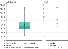
Figure 1: Boxplots for overnight construction costs and time

The right boxplot in Fig. 1 presents a similar image for construction time. Future projections range from 5 to 9 years, but recent and ongoing projects are currently taking 10 to 17 years. These overruns drive up financing costs and can also threaten energy security.

Table 1: Parameters for nuclear power

Parameter	Unit	Value / Range
Overnight construction cost	US-$/kW	1,914 - 12,600
Annual fixed operational cost	US-$/kW	88.81
Variable operational cost (incl. fuel)	US-$/MWh	10.96
Capacity factor	%	95
Construction time	years	4 - 10
Depreciation period	years	40

Together, construction and financing costs constitute total construction costs (TCC). Financing costs reflect the interest paid and are typically calculated from the length of depreciation and the interest rate. Following the methodology for nuclear power investments introduced in (Rothwell, 2016), our analysis additionally accounts for costs during construction. We compute the financing costs during construction $f$ using Equation 1 introduced by Rothwell (2016). In the equation $i$ is the interest rate, $t$ the construction time, and $c$ the overnight construction costs.

$$f=(\frac{i}{2\cdot t}+\frac{i^{2}}{6\cdot t^{2}})*c$$ (1)

For the comparison of LCOEs and analysis with the energy system model, the annuity $a$ is computed for the sum of financing and overnight construction costs according to Equation 2. In the formula, $d$ is the depreciation period.

$$a=(f+c)\cdot\frac{(1+i)^{d}\cdot i}{(1+i)^{d}-1}$$ (2)

Finally, the LCOE $l$ for a single year corresponds to the sum of annuity and variable costs $v$ divided by the yearly generation. The yearly generation corresponds to the product of the utilization rate $u$ and the numbers of hours in a year.

$$l=\frac{a+v\cdot u\cdot 8760}{u\cdot 8760}$$ (3)

2.2 Energy system model

The deployed planning model decides on the resources and technologies to supply an exogenous demand for energy services. Fig. 2 provides an overview of the considered primary energy sources, secondary energy carriers, and the categories for final demand. Besides nuclear power, supply of primary energy is restricted to renewable sources, namely wind, hydro, photovoltaic, and biomass. To capture intermediate steps between final demand and primary supply, the model includes secondary carriers, like hydrogen or synthetic gas and oil. Finally, the model must meet the demand for residential and industrial heat, passenger and freight transport, synthetic fuels for aviation and navigation, and electricity.

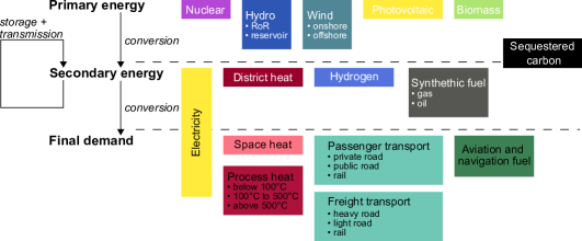
Figure 2: Overview of model structure

To cover final demand, the model decides on the expansion and operation of predefined technologies. Technologies in the model generate, convert, store, or transport energy carriers or provide an energy service. For instance, wind turbines generate electricity that can either satisfy the final electricity demand, be temporarily stored by a battery or be converted to hydrogen by an electrolyzer or to heat by a heat pump to satisfy final demand. Overall, the model includes 22 energy carriers and 125 distinct technologies. Except for nuclear, the choice and parametrization of technologies is based on reports of the Danish Energy Agency (2022) and on Robinius et al. (2020) for the transport sector. The graph in Fig. 3 shows all technoloiges supplying electricity. In the graph, vertices either represent energy carriers, depicted as colored squares, or technologies, depicted as gray circles. Entering edges of technologies refer to input carriers; outgoing edges refer to outputs. The appendix C provides a comprehensive graphs with all considered technologies.

Figure 3: Technologies for electricity supply

The model’s objective is to minimize the total system costs which consist of annualized expansion and operational costs for technologies and costs of energy imports from outside the system. Accordingly, the model takes a strictly techno-economic social planner approach and does not consider the different agents within the system, such as producers, consumers, or governments, and their behavior. The model is formulated as a linear optimization problem without constraints on unit commitment. Therefore, operational restrictions, e.g., ramping rates or start-up times, for nuclear power, or any other technology, are neglected. Previous studies agree that operational detail has little impact on results if models include options for short-term flexibility, like batteries or demand-side response (Poncelet et al., 2016, 2020). In addition, most technologies subject to considerable operational restrictions are excluded from our analysis, for instance coal power plants. As a result, the approach only creates a positive bias in favor of nuclear power, which is in line with our intention to compute an upper bound on its deployment.

The temporal scope of the model consists of a single year. Using a brownfield approach, today’s transmission infrastructure is available without further investment due to its long technical lifetime. In addition, the model can decide to invest into additional infrastructure. The same applies to all kinds of hydro power plants. Additional transmission capacities and all other technologies require investment to be available. Technology and demand data is based on projections for the year 2040. The model uses an hourly temporal resolution for electricity to capture fluctuations of renewables and the sensitivity of the power grid to imbalances. For other energy carriers, the model uses a coarser but at least daily resolution to reduce computational load and capture the inherent flexibility (Göke, 2021). For instance, hydrogen uses a daily resolution to capture its physical inertia and the resulting storage capabilities of pipelines. The resolutions used for other carriers are discussed in the section below.

For timeseries of electricity demand, heat demand, and renewable supply, the model uses historic data from 2008. Since the scope only includes a single climatic year, planning does not consider extreme events with low renewable supply but high demand. On the other hand, we neither consider the risk of coincident nuclear outages threatening security of supply, for instance during the Winter of 2022/2023 in France (New York Times, 2022).

2.2.1 Spatial resolution and starting grid

The map in Fig. 4 shows the spatial resolution of the model. The spatial scope includes the European Union plus the United Kingdom, Switzerland, Norway, and the entire Balkan region. The spatial resolution of the model divides this scope into 96 clusters with distinct energy balances and capacities.

Figure 4: Pre-existing grid infrastructure (solid) and new potential connections (dashed) in the model

Representation of the electricity grid distinguishes HVAC and HVDC grids and aggregates clusters according to the balancing zones of the European power market. On the one hand, this resolution neglects interzonal congestions, but on the other hand, it allows to build on specific ENTSO-E data on limits and costs for the expansion of net-transfer capacities in the European power grid ENTSO-E (2020). More detailed resolutions must rely on unspecific cost assumptions that range from 400 to 1,000 EUR per MW and km (Fürsch et al., 2013; Gerbaulet and Lorenz, 2017). Neglecting interzonal congestions does not impose a bias in favor of renewables and against nuclear power since nuclear capacities are typically centralized in remote areas and require substantial interzonal connection with demand centers. For renewables this is only partially true: While onshore and especially offshore wind depend on transmission grids, too, PV can be built very close to demand. In addition, we use a transport instead of flow formulation for power grid operation since previous research found this simplification to be sufficiently accurate (Neumann et al., 2022).

To exchange hydrogen between clusters, the model can build transmission infrastructure between neighboring clusters, or overseas in plausible cases. These pipelines are subject to costs of 0.4 million EUR per GW and km and energy losses of 2.44% per 1,000 km (Danish Energy Agency, 2022). The distance between the geographic center of clusters serves as an estimate for pipeline length.

2.2.2 Flexibility and electricity demand

Nuclear power has a key advantage over renewable wind or PV—it is dispatchable. In our analysis, nuclear plants are considered to be fully flexible and are not subject to operational restrictions. To what extent these characteristic drives investment strongly depends on if and how a model includes alternatives to nuclear for the provision of flexibility. One flexibility option, the interconnection of regions, is covered by the large spatial scope and consideration of transmission infrastructure in our model. This section details the representation of two additional options: energy storage and flexible demand.

First, the model includes several technologies for electricity storage. It can invest in batteries or utilize the pre-existing pumped storage and reservoir plants. Second, and more importantly, the model considers investment into storage technologies for other carriers, too. Tanks and caverns for hydrogen storage decouple electricity consumption by electrolyzers from hydrogen demand adding substantial flexibility since the modeled system requires a great amount of hydrogen for high temperature process heat and synthetic aviation fuels. In addition, using stored hydrogen for electricity generation provides an option for long-term storage that batteries or pumped storage cannot. Finally, the model includes different technologies for heat storage. At additional investment costs, electric heating systems on the consumer level can be equipped with short-term heat storages to mitigate load peaks. In heating networks storage options include water tanks for short and thermal pits for long storage durations.

Beyond storage, the model captures to what extent final demand is elastic and can adapt to supply. To represent this, it varies temporal resolution by energy carrier. For the final demand for electricity, we assume no elasticity and use an hourly resolution.

The demand for residential and industrial heat uses a 4-hour resolution, but the generation profile of each individual heating system on the consumer level is fixed to match demand. Technologies within heating networks can instead operate flexible but must jointly meet the final demand of the connected consumers, similar to the power grid. In residential heating, the 4-hour resolution captures the thermal inertia of buildings (Heinen et al., 2017); in heating networks the inertia of the network itself (Triebs and Tsatsaronis, 2022); and in industrial heating the possibility to reschedule processes. It should be noted that despite the 4-hour resolution, industrial heating is mostly inflexible in this approach, because demand is almost constant, and systems must continuously operate close to full capacity.

Demand from BEVs is flexible within limits: First, an hourly profile restricts charging and reflects when BEVs are connected to the grid. Second, for each day the sum of charged electricity must match consumption. To implement the latter, transport services use a daily resolution in the model. This approach is a compromise regarding the flexibility of BEVs in future power systems which is still subject to significant uncertainty. On the one hand, we assume charging can be flexible to some degree and can adapt to supply (Strobel et al., 2022). On the other, we do not consider bidirectional loading, also known as vehicle-to-grid, where BEVs can operate like regular batteries and supply energy back to the grid (Hannan et al., 2022). Apart from BEVs, other electricity consumption in the transport sector, for instance for rail transport, is inflexible and uses an hourly resolution.

2.2.3 Renewable supply

In the model, the level of investment into nuclear power depends on the potential and costs of its alternative renewable energy. Therefore, this section provides further details on the used assumptions regarding renewable supply.

Assumptions on the technical potential of wind and solar can vary substantially. In our study, we use data from Auer et al. (2020) for the potential of wind and solar. To put these numbers into context, we compare them against results of a meta-analysis on renewable potential in Germany in the appendix D (Risch et al., 2022). The material demonstrates that the assumed potential is in line with results of the meta-analysis, except for PV, for which our assumptions are more conservative.

To reflect that sites for renewables differ in quality, wind and PV technologies are further subdivided. Onshore wind and openspace PV each have three sub-technologies; rooftop PV has two. Energy yield and capacity potential for each sub-technology are computed for each of the 96 clusters based on the respective distribution of full-load hours. Offshore wind is subdivided into two technologies with identical full-load hours, but different investment costs representing shallow and deep waters. Figures in section D of the appendix sort the entire potential of different renewables by full-load hours and demonstrate how increased deployment results in smaller yields.

The use of biomass in each country is subject to an upper energy limit that sums to 1,081 TWh for the entire model (Institute for Energy and Transport (2015), Joint Research Center). In addition to domestic production, the model can import renewable hydrogen by ship at costs of 131.8 US-$₂₀₁₈ per MWh and by pipeline from Marocco or Egypt at 90.7 and 86.8 US-$₂₀₁₈ per MWh, respectively (Hampp et al., 2021).

3 Results

This section 3 first compares the computed range of LCOEs for nuclear power with renewable sources. Afterwards, we present the results of the more elaborate analysis applying the energy planning model.

3.1 Levelized cost comparison

Based on the review of construction projections, we compute a conceivable range for LCOE for nuclear power using the formula presented in section 2.1. Fig. 5 compares this range against historic LCOEs on the left side (a) and against cost projections for renewable energy on the right (b). Historic LCOEs for all energy sources build on the corresponding reports by Lazard Ltd from 2009 to 2021. The projection for nuclear results from the parameters in Table 1, projections for renewable sources use 2040 data from Danish Energy Agency (2022) for cost assumptions and the 10th to 90th percentile of respective energy yield in Europe for full-load hours. For a full documentation of assumptions on costs and renewable potential, see the respective sections in the appendix A and B.

Figure 5: Comparison of LCOEs for generation technologies

The comparison of historic LCOEs shows how, in the past, costs for nuclear power increased but dropped for renewable energy, in particular for PV. Current costs for nuclear power reported by Lazard are at the upper end of our projections for the future. For wind, current costs are already within the project range; for PV, current costs are above projections implying a continuous degression of costs. Overall, the comparison of projected LCOEs suggests that nuclear can only compete with renewables if the industry can reverse the historic trend and achieve substantial learning effects and economies of scale to reduce project costs.

3.2 Planning model analysis

However, comparing LCOEs for nuclear and renewables is of limited insight because nuclear and renewables ultimately provide different goods: nuclear plants are dispatchable and can, within limits, adapt supply to demand; renewable energy sources like wind and PV cannot. Therefore, we elaborate our comparison and deploy a techno-economic planning model of the European energy system for further analysis. The model captures fluctuations of wind and PV and assumes fully flexible operation of nuclear plants. Its objective is to minimize the sum of investment and operational costs for meeting energy demand in a fully decarbonized system.

Fig. 6 presents the key results of the energy system model analysis. On the left axis, the graph shows the share of nuclear power in total electricity generation depending on the overnight construction costs and time. The right axis provides the corresponding distribution of cost projections in the literature and actual costs reported by recent projects.

Figure 6: Generation share of nuclear and distribution of overnight cost projections

The results confirm the tentative conclusion from the LCOE analysis. Only if construction costs and time drop substantially, nuclear power provides a significant share of electricity. At 7 years construction time, overnight costs must drop to 4,120 US-$ per kW to achieve a 10% share in generation, at 4 years construction time this threshold increases to 4,450 US-$ per kW. At the same time, only 20% of overnight construction cost projections are below 4,120 US-$ per kW and actual costs of recent projects lie above 7,500 US-$ per kW. At the lowest construction costs, projected by OECD and NEA (2018), nuclear power provides up to 52 % of total electricity generation. Non-nuclear electricity generation largely corresponds to wind and PV. Other sources are hydro which is kept at today’s level supplying 540 TWh. Biomass supplies at most 13.6 TWh since the model predominantly deploys the limited potential to cover the demand for synthetic fuels instead.

Despite its assumed flexibility, nuclear power rather substitutes than complements fluctuating supply from wind and PV generation. In the most extreme case with a 52 % generation share, nuclear power plants are operating at a utilization rate of 94.4%; close to the 95% limit. This changes only slightly at smaller nuclear and consequently higher renewable shares. At a nuclear share of 7.9%, utilization still amounts to 88.7%, which is above the average of European nuclear plants operating today (Wealer et al., 2021). This implies that even if technically capable, nuclear power is economically not well suited to provide system flexibility due to its high investment costs.

To highlight the system’s renewable integration, Fig. 7 exemplarily compares the residual load curves of Germany for a system with the highest nuclear share of 52% and no nuclear capacity at all. Residual load is the remaining electricity demand after subtracting supply of fluctuating renewables from total demand. Plotted in descending order, the curve shows the residual peak load on the y-axis, the amount of residual demand as the area above the x-axis, and excess energy as the area below the x-axis. Appendix F shows an extract of the hourly model results from which the duration curves were computed.

Figure 7: Residual load curve for Germany in a system with a nuclear share of 52% (left) and no nuclear at all (right)

In the graphs, there are two residual load curves: ’Flexible demand’ shows the actual residual load in the model; ’inflexible demand’ is computed ex-post assuming demand cannot adapt to supply. To what extent demand is flexible depends on its use. The conventional final demand for electricity is inflexible, but only constitutes around 39% of total demand, exact shares differing from case to case. Additionally, the creation of synthetic fuels takes up 24%, electrified transportation 20% and heating 17% of total electricity demand. This demand can be flexible within specific restrictions detailed in Section 2. Some of this flexibility comes without costs, like flexible charging of battery electric vehicles, but most require the model to invest, for instance into heat or hydrogen storage.

In the 52% nuclear system, wind and PV only account for 10% of generation in Germany and the need for flexibility is small. The residual load is flat and does not substantially adapt to supply. For the system without nuclear, results are contrary. To reduce the amount of residual demand and excess energy, demand substantially adapts to supply. For instance, electrolyzers operate more flexibly, thereby causing their full-load hours to decrease to 3,343 compared to 5,979 in the 52% nuclear system while more than doubling their capacity from 35.9 to 77.1 GW. Investments in heat and hydrogen storage provide additional flexibility. Storage capacities for district heating increase to 40.9 TWh compared to 18.2 Twh in the 52% nuclear system; for hydrogen even to 12.4 from 1.7 TWh.

Coloured areas in the graph indicate how the system covers the residual load. In the 52% nuclear system, 132 GW of nuclear operate at full capacity and cover the predominant share of residual load. Additional imports of 86.9 TWh from neighboring countries cover peak loads. Vice versa, Germany exports 78.5 TWh of excess supply. In the system without nuclear, the residual load is smaller, but imports are higher and cover 244 TWh of demand—the predominant share of residual load. Dispatchable thermal plants fueled by hydrogen and biogas only provide 7.3 TWh of generation. In both cases, there is no additional investment in electricity storage and both systems only deploy the existing pumped storage and hydro reservoirs.

Although the integration of renewables requires additional investments, nuclear power is only a cost-efficient alternative at very low construction costs as shown previously. Otherwise, investment costs of nuclear significantly outweigh the costs of renewables and corresponding flexibility options. For instance, the system without nuclear shows 9.7 billion US-$ of additional annualized investment into demand side flexibility compared to the 52% nuclear system. Adding 8.2 billion US-$ for additional grid infrastructure and 3.0 billion US-$ for thermal plants, total costs of renewable integration add up to 20.9 billion US-$. But on the other hand, even if overnight construction costs of nuclear drop to 5,430 US-$ per kW, the median of projections in Fig. 6, the 52% nuclear system is already 46.9 billion US-$ more expensive than the system without nuclear. This 46.9 billion US-$ difference is composed of a 67.8 billion US-$ increase in generation costs only partially offset by 20.9 billion US-$ of additional integration costs in the system without nuclear exclusively deploying renewables. For reference, the total costs of renewable generation amount to 150.5 billion US-$ in this case.

Fig. 8 further investigates the role of import and export for both systems. It shows electricity generation and net exchange of hydrogen and electricity by high-voltage alternating current (HVAC) or direct current (HVDC) grids for each country. Exchange of hydrogen and electricity increases substantially in the system without nuclear reflecting the 8.2 billion US-$ rise of costs for grid infrastructure. The maps show that this infrastructure not only serves renewable integration but reduces generation costs as well because it allows to utilize renewables where full-load hours are highest, for instance in southern Europe for PV or in the North Sea for offshore wind.

Figure 8: Electricity generation and exchange the 52% nuclear system (top) and the system without nuclear (bottom)

For a comprehensive overview of energy flows and conversion processes in the compared energy systems, see appendix H.

4 Discussion

Although building on an extensive review of cost projections and a detailed planning model, our analysis faces some inevitable limitations. Overall, these limitations impose a positive bias on nuclear power, so results are rather an upper bound than reliable estimates for the cost-efficient share of nuclear.

First, there are simplifications of the techno-economic model itself. We consider construction cost of nuclear (and all other technologies) as exogenous, although costs can depend on the level of investment due to learning effects. Therefore, cases in Fig. 6 with low nuclear shares, but construction costs dropping below 5,000 US-$ per kW, are implausible. If learning can in fact achieve such a drop in costs, it will require capacity investments that will already raise the share of nuclear in power generation above 10%. To achieve this share, 41 GW of nuclear would have to be built which approximately corresponds to 25 EPR-sized reactors. A nuclear share of 50% requires 132.5 GW of capacity, i.e. 83 EPR-sized reactors. Given the current state of ongoing projects in France, Finland and the UK, this seems rather challenging (Rothwell, 2022). Considering learning effects endogenously is not an option, due to the uncertainty of their existence and computational limits (Berthélemy and Escobar Rangel, 2015; Grubler, 2010; Harding, 2007).

The model focuses on the single year 2040, but decarbonization of the energy system is a process over several decades. Computational limits however require to limit the analysis to one year. On the one hand, this year should be sufficiently far in the future to allow for learning effects of nuclear. On the other hand, years further into the future will increasingly favor renewables since learning effects are expected to keep reducing their costs, too (Danish Energy Agency, 2022). Against this background, we choose 2040 as the earliest date until that substantial reductions of costs are conceivable, an optimistic assumption considering the construction times of recent European nuclear projects.

On the more technical side, we omit unit commitment constraints, as already mentioned. Of all considered technologies, these operational restrictions are most pronounced for nuclear power. The method section discusses further technical limitations like the representation of extreme events and grid constraints.

Second, some adverse characteristics of nuclear power escape the techno-economic perspective of the analysis. For instance, costs of managing nuclear waste and decommissioning old plants are substantial but not included in our analysis due to unavailability of reliable data and the long time frame (Lordan-Perret et al., 2021; Lovins, 2022). Furthermore, nuclear power carries the risk of severe accidents, proliferation of nuclear material and radioactive contamination (Lévêque, 2014; Wheatley et al., 2016; Lehtveer and Hedenus, 2015). Although robust quantification of these externalities is difficult and therefore not part of the analysis, their social costs typically exceed estimates for renewable energy (Stirling, 1997).

5 Conclusion and Policy Implications

Our least-cost analysis indicates that nuclear power is only a cost efficient option for full decarbonization of Europe’s energy system if construction costs at least half and drop below 4,000 US-$₂₀₁₈ per kW. In contrast, costs and construction time for nuclear power in the last ten years have been increasing rather than decreasing. This assessment uses optimistic assumptions for other characteristics of nuclear, like availability and operational costs, and still omits social costs, like the risk of accidents or waste management, since these externalities escape robust quantification.

Results show that nuclear power reduces investments into system flexibility. Since nuclear plants are, in contrast to wind or PV, dispatchable, their system integration induces lower costs for grid infrastructure, energy storage, demand-side flexibility, or thermal backup plants. However, if generation costs of nuclear do not drop substantially, they outweigh this benefit. For instance, assuming overnight construction costs of 5,430 US-$ per kW, the median of compiled projections, a 52% generation share of nuclear will reduce investments into system flexibility by 20.9 bn US-$ per year but increase generation costs by 67.8 bn US-$ or 44% compared to a fully renewable system.

A crucial detail to understand these results is that apart from grid infrastructure, most investments into system flexibility occur outside of the power sector. Instead of battery storage or conventional demand-side management, new electricity demand induced by the decarbonization of heating, transport, and industry adds substantial flexibility. For instance, hydrogen production, accounting for 25% of electricity demand, supports renewable integration by adapting to renewable supply and using storage to match production with demand.

Results do not indicate that fluctuating renewables and flexibly operated nuclear plants are economic complements. Even when neglecting operational restrictions, nuclear power runs at utilization rates close to 90%. From a cost perspective, it is preferable to invest into system flexibility rather than running capital-intensive nuclear plants at low utilization rates.

Our analysis puts previous least-cost analyses on nuclear power that were limited to the power sector and a single country into perspective. As we showed, this setup omits two key options for system integration of fluctuating renewables: First, grid infrastructure connecting regions with different generation profiles, and second, the potential flexibility of electricity demand added to decarbonize the heating, transport, and industry sector. As a result, previous analyses overestimated the value of dispatchable nuclear power plants. Not considering other types of firm generation, like hydrogen or biogas fueled plants, adds to this bias.

Our results suggest that efforts to advance nuclear technology—if undertaken at all—should focus on reducing costs and construction time. If plans to extend nuclear capacity are followed through, and renewable investments consequently neglected, project construction delays might put European energy security at risk. Concepts for more flexible operation are not promising because even fully flexible plants almost exclusively operate at full capacity for economic reasons. Since the share of nuclear also affects investments into grid infrastructure and energy storage, path dependencies in system development arise. The risk of nuclear power not achieving substantial cost reductions should thus be accounted for in long-term planning. Potential non-electrical applications for nuclear power, such as high temperature provision for industrial processes, are not considered in this paper but should be addressed in future research.

Supplementary material

All data and running scripts used in this paper are openly available here: https://github.com/leonardgoeke/EuSysMod/tree/greenfield_nu Due to their size, model outputs are not part of the repository but are available upon request.

The applied model uses the open AnyMOD.jl modeling framework (Göke, 2021). The applied version of the tool is openly available under this link. https://github.com/leonardgoeke/AnyMOD.jl/releases/tag/flexibleElectrificationWorkingPaper

6 Acknowledgments

The research leading to these results has received funding from the Deutsche Forschungsgemeinschaft (DFG) under project number 423336886.

Appendix A Review of other parameters

Table 14 show how future projections for overnight construction costs are substantially below recently reported costs. Table 13 compares the costs of different reactor types. Table 15 provides the factors for inflation adjustments normalized to 2018 following inflationtool.com.

Figure 9: Boxplot diagram for for capacity factors, construction time, fuel cost, operational lifetime, efficiency and combined O&M cost

Table 2: Unfiltered overnight construction costs for nuclear plants.

Reference	Page	Cost Description	Reactor	Reference Year	Capacity in kW	OCC	Unit
Barkatullah and Ahmad (2017)	132	Asssumed parameters	n.a.	2017	n.a.	4646	US-$(2018) per kWe
Boldon and Sabharwall (2014)	19	Input Water-Cooled SMR	SMR	2014	1260	3767	US-$(2011) per kW
Stein et al. (2022)	30	Lower Cost, High Learning (Best Case) // FOAK CAPEX	Traditional Nuclear	2020	n.a.	4783	US-$(2020) per kWe
Stein et al. (2022)	30	Lower Cost, High Learning (Best Case) // FOAK CAPEX	SMR	2020	n.a.	5108	US-$(2020) per kWe
Stein et al. (2022)	30	Lower Cost, High Learning (Best Case) // FOAK CAPEX	HTGR	2020	n.a.	5518	US-$(2020) per kWe
Stein et al. (2022)	30	Lower Cost, High Learning (Best Case) // FOAK CAPEX	Advanced reactor with thermal storage (ARTES)	2020	n.a.	4000	US-$(2020) per kWe
Stein et al. (2022)	30	Upper Cost, Low Learning (Worst Case) // FOAK CAPEX	Traditional Nuclear	2020	n.a.	6338	US-$(2020) per kWe
Stein et al. (2022)	30	Upper Cost, Low Learning (Worst Case) // FOAK CAPEX	SMR	2020	n.a.	6974	US-$(2020) per kWe
Stein et al. (2022)	30	Upper Cost, Low Learning (Worst Case) // FOAK CAPEX	HTGR	2020	n.a.	7500	US-$(2020) per kWe
Stein et al. (2022)	30	Upper Cost, Low Learning (Worst Case) // FOAK CAPEX	Advanced reactor with thermal storage (ARTES)	2020	n.a.	6220	US-$(2020) per kWe
Dixon et al. (2017)	xii	Mean Costs	Thermal LWR Reactor	2017	n.a.	4300	US-$(2017) per kW
Dixon et al. (2017)	xii	Mean Costs	Fast Reactors	2017	n.a.	4700	US-$(2017) per kW
Dixon et al. (2017)	xii	Mean Costs	Gas-cooled reactors	2017	n.a.	5170	US-$(2017) per kW
Dixon et al. (2017)	xii	Mean Costs	PHWR	2017	n.a.	4230	US-$(2017) per kW
Duan et al. (2022)	2	Capital Costs	US nuclear	n.a.	n.a.	4000	US-$ per kW
Duan et al. (2022)	2	Capital Costs	US nuclear	n.a.	n.a.	6317	US-$ per kW
Green (2019)	18	HTGR	SMR	2016	250	5000	US-$ per kW
Green (2019)	18	CAREM25	SMR	2017	25	21900	US-$ per kW
Green (2019)	21	Median (Low)	SMR	2013	45	4000	US-$ per kW
Green (2019)	21	Median (High)	SMR	2013	45	16300	US-$ per kW
Green (2019)	21	Median (Low)	SMR	2013	225	3200	US-$ per kW
Green (2019)	21	Median (High)	SMR	2013	225	7100	US-$ per kW
Grubler (2010)	5179	Capital Costs France with no cost increase since 1998	French PWR	1998	n.a.	2600	US-$(2008) per kWe
Grubler (2010)	5179	Capital Costs France with no cost increase since 1998	French PWR	1998	n.a.	2100	US-$(2008) per kWe
International Atomic Energy Agency (2020)	56	SMART (FOAK)	SMR	2020	30	10000	US-$ per kW
IEA et al. (2020)	49	Nuclear New Build - France	EPR	2019	1650	4013	US-$ per kW
IEA et al. (2020)	49	Nuclear New Build - Japan	ALWR	2019	1152	3963	US-$ per kW
IEA et al. (2020)	49	Nuclear New Build - Korea	ALWR	2019	1377	2157	US-$ per kW
IEA et al. (2020)	49	Nuclear New Build - Russia	VVER	2019	1122	2271	US-$ per kW
IEA et al. (2020)	49	Nuclear New Build - Slovak Republic	Other nuclear	2019	1004	6920	US-$ per kW
IEA et al. (2020)	49	Nuclear New Build - United States	LWR	2019	1100	4250	US-$ per kW
IEA et al. (2020)	49	Nuclear New Build - China	LWR	2019	950	2500	US-$ per kW
IEA et al. (2020)	49	Nuclear New Build - India	LWR	2019	950	2778	US-$ per kW
Lazard Ltd (2021)	18	Nuclear (New Build, Low Case)	n.a.	2021	2200	7800	US-$(2022) per kWe
Lazard Ltd (2021)	18	Nuclear (New Build, High Case)	n.a.	2021	2200	12800	US-$(2022) per kWe
MIT (2018)	236	Overnight Costs (Standard LWR)	LWR	2018	n.a.	5000	US-$(2017) per kWe
MIT (2018)	70	Total Overnight Costs	Molten Salt Reactor	2018	2275 (MWth)	5400	US-$(2017) per kW
MIT (2018)	236	FOAK CAPEX	HTGR	2017	n.a.	5200	US-$(2017) per kW
MIT (2018)	159, 220	Benchmark Scenario Cost	Nuclear	2018	n.a.	4900	US-$(2017) per kW
MIT (2018)	220	Barakah OCC	APR1400	2010	n.a.	4000	US-$(2017) per kW
MIT (2018)	149	US (high)	Nuclear	2018	1000	6880	US-$(2017) per kW
MIT (2018)	149	US (nominal)	Nuclear	2018	1000	5500	US-$(2017) per kW
MIT (2018)	149	US (low)	Nuclear	2018	1000	4100	US-$(2017) per kW
MIT (2018)	149	US (very low)	Nuclear	2018	1000	2750	US-$(2017) per kW
MIT (2018)	150	China (nominal)	Nuclear	2018	1000	2800	US-$(2017) per kW
MIT (2018)	150	China (low)	Nuclear	2018	1000	2080	US-$(2017) per kW
MIT (2018)	151	France (nominal)	Nuclear	2018	1000	6800	US-$(2017) per kW
MIT (2018)	151	France (low)	Nuclear	2018	1000	5070	US-$(2017) per kW
MIT (2018)	150	UK (nominal)	Nuclear	2018	1000	8140	US-$(2017) per kW
MIT (2018)	150	UK (low)	Nuclear	2018	1000	6070	US-$(2017) per kW
Laboratory (2016)	46	LCOE build-up for GWe LWR	LWR	n.a.	n.a.	26.99	US-$ per MWh
NREL (2021)	Xls Sheet "Nuclear"	Nuclear-Moderate	Nuclear	2019	n.a.	6297	US-$(2019) per kWe
OECD and NEA (2018)	68	Nuclear (min)	n.a.	2020	535	1807	US-$(2015) per kWe
OECD and NEA (2018)	68	Nuclear (mean)	n.a.	2020	1343	4249	US-$(2015) per kWe
OECD and NEA (2018)	68	Nuclear (median)	n.a.	2020	1300	4896	US-$(2015) per kWe
OECD and NEA (2018)	68	Nuclear (max)	n.a.	2020	3300	6215	US-$(2015) per kWe
Rothwell (2016)	106	FOAK, no sec	SMR	2013	360	7343	US-$ per kW
Rothwell (2016)	106	NOAK, no sec	SMR	2013	360	5357	US-$ per kW
Rothwell (2016)	106	FOAK, sec = 0.1%	SMR	2013	360	6722	US-$ per kW
Rothwell (2016)	106	NOAK, sec = 0.1%	SMR	2013	360	4885	US-$ per kW
Rothwell (2022)	2	Taishin 1 & 2, China	EPR	2019	1600	3200	US-$(2018) per kWe
Rothwell (2022)	2	Sanmen, China	AP1000	2018	1150	3270	US-$(2018) per kWe
Rothwell (2022)	6	NuScale NOAK	SMR	2022	n.a.	3600	US-$(2018) per kWe
Rothwell (2022)	4	Belgium	EPR	2015	1600	5515	US-$(2018) per kWe
Rothwell (2022)	4	UK	EPR	2015	1600	6588	US-$(2018) per kWe
Rothwell (2022)	4	Hungary	VVER1200	2015	1200	6745	US-$(2018) per kWe
Rothwell (2022)	2	Olkiluoto, Finland	EPR	2020	1600	7600	US-$(2018) per kWe
Rothwell (2022)	6	NuScale FOAK	SMR	2022	n.a.	8000	US-$(2018) per kWe
Rothwell (2022)	2	Hinkley Point, Uk	EPR	2019	1600	9300	US-$(2018) per kWe
Rothwell (2022)	2	Vogtle Station, US	AP1000	2021	1150	12000	US-$(2018) per kWe
Rothwell (2022)	6	TerraPower FOAK	SMR	2022	n.a.	12000	US-$(2018) per kWe
Rothwell (2022)	2	Flamanville, France	EPR	2020	1600	12600	US-$(2018) per kWe
Shirvan (2022)	7	10th unit AP1000 (Should cost)	AP1000	2019	1150	2900	US-$(2018) per kWe
Shirvan (2022)	7	Next AP1000 (Should cost)	AP1000	2019	1150	4300	US-$(2018) per kWe
Shirvan (2022)	7	10th unit AP1000 (Post-COVID high estimate)	AP1000	2022	1150	4500	US-$(2022) per kWe
Shirvan (2022)	7	Historic (Pre-Three-Mile-Island)	PWR	1979	1200	4700	US-$(2018) per kWe
Shirvan (2022)	7	Next AP1000 (Post-COVID high estimate)	AP1000	2022	1150	6800	US-$(2022) per kWe
Shirvan (2022)	7	Vogtle Station, US (Official)	AP1000	2021	1150	7956	US-$(2018) per kWe
Shirvan (2022)	7	Vogtle Station, US (Independent)	AP1000	2022	1150	9200	US-$(2018) per kWe
Shirvan (2022)	7	Historic (Post-Three-Mile-Island)	PWR	>1979	1200	9512	US-$(2018) per kWe
Stewart and Shirvan (2021)	13	FOAK (US)	Large Passive Safety PWR	2018	n.a.	4328	US-$(2018) per kWe
Stewart and Shirvan (2021)	13	FOAK (China) (min)	Large Passive Safety PWR	2018	n.a.	1700	US-$(2018) per kWe
Stewart and Shirvan (2021)	13	FOAK (China) (max)	Large Passive Safety PWR	2018	n.a.	2200	US-$(2018) per kWe
Stewart and Shirvan (2021)	13	First-4 unit average	Large Active Safety PWR	2018	n.a.	5337	US-$(2018) per kWe
Stewart and Shirvan (2021)	13	APR1400 4-unit average - Barakah	APR1400	2018	n.a.	4358	US-$(2018) per kWe
Stewart and Shirvan (2021)	13	10th of a kind	SMR	2018	n.a.	3856	US-$(2018) per kWe
Tolley et al. (2004)	7	No-Policy Nuclear LCOE Installations (Max OCC)	Advanced Nuclear Reactor	2003	1000	1800	US-$(2003) per kW
Wealer et al. (2021)	5	Inputs for MC	n.a.	2018	1600	4000-9000	US-$(2018) per kWe

Table 2: (continued)

Table 3: Overnight construction costs reported for LWR in OECD countries.

Reference	Cost Description	Cost in US-$(2018) per kW
Lazard Ltd (2021)	Nuclear (New Build, High Case)	10883.42828
Lazard Ltd (2021)	Nuclear (New Build, Low Case)	6632.089108
Rothwell (2022)	Flamanville, France	12600
Rothwell (2022)	Hinkley Point, Uk	9300
Rothwell (2022)	Olkiluoto, Finland	7600
Rothwell (2022)	Vogtle Station, US	12000
Shirvan (2022)	Historic (Post-Three-Mile-Island)	9512
Shirvan (2022)	Historic (Pre-Three-Mile-Island)	4700
Shirvan (2022)	Vogtle Station, US (Independent)	9200
Shirvan (2022)	Vogtle Station, US (Official)	7956

Table 4: Overnight construction costs projected for LWR in OECD countries.

Reference	Cost Description	Cost in US-$(2018) per kW
Barkatullah and Ahmad (2017)	Asssumed parameters	4646
Stein et al. (2022)	Lower Cost, High Learning (Best Case) // FOAK CAPEX	4640.535558
Stein et al. (2022)	Upper Cost, Low Learning (Worst Case) // FOAK CAPEX	6149.218977
Dixon et al. (2017)	Mean Costs	4404.92
Duan et al. (2022)	Capital Costs 1	4000
Duan et al. (2022)	Capital Costs 2	6317
IEA et al. (2020)	Nuclear New Build - France	3941.656026
IEA et al. (2020)	Nuclear New Build - Japan	3892.544937
IEA et al. (2020)	Nuclear New Build - Korea	2118.652392
IEA et al. (2020)	Nuclear New Build - Slovak Republic	6796.974757
IEA et al. (2020)	Nuclear New Build - United States	4174.442589
MIT (2018)	Benchmark Scenario Cost	5019.56
MIT (2018)	France (low)	5193.708
MIT (2018)	France (nominal)	6965.92
MIT (2018)	Overnight Costs (Standard LWR)	5122
MIT (2018)	UK (low)	6218.108
MIT (2018)	UK (nominal)	8338.616
MIT (2018)	US (high)	7047.872
MIT (2018)	US (low)	4200.04
MIT (2018)	US (nominal)	5634.2
MIT (2018)	US (very low)	2817.1
NREL (2021)	Nuclear-Moderate	6185.050584
OECD and NEA (2018)	Nuclear (max)	6584.171
OECD and NEA (2018)	Nuclear (mean)	4501.3906
OECD and NEA (2018)	Nuclear (median)	5186.8224
OECD and NEA (2018)	Nuclear (min)	1914.3358
Rothwell (2022)	Belgium	5515
Rothwell (2022)	Hungary	6745
Rothwell (2022)	UK	6588
Shirvan (2022)	10th unit AP1000 (Post-COVID high estimate)	3826.205255
Shirvan (2022)	10th unit AP1000 (Should cost)	2900
Shirvan (2022)	Next AP1000 (Post-COVID high estimate)	5781.821274
Shirvan (2022)	Next AP1000 (Should cost)	4300
Stewart and Shirvan (2021)	First-4 unit average	5337
Stewart and Shirvan (2021)	FOAK (US)	4328
Wealer et al. (2021)	Inputs for MC MAX	9000
Wealer et al. (2021)	Inputs for MC MIN	4000

Table 4: (continued)

In literature, operation & maintenance (O&M) costs are often provided as two components. The first component, fixed O&M costs, does not depend on yearly generation quantities, but the second component, variable O&M costs, does and is given in US-$/MWh. Some references however only provide one component, e.g., Budi et al. (2019); Ingersoll et al. (2020); International Atomic Energy Agency (2020), for a detailed overview see Table LABEL:tab:opex_unfiltered.

To make literature O&M cost comparable, we combine fixed and variable costs to a single value in US-$/kW. For this, we assume an optimistic 95% capacity factor to determine nuclear full load hours and are thus able to determine combined O&M costs for all references. Hereby, we also caclulate the average ratio of fixed and variable costs to then determine the average fixed and variable O&M costs from the 25%-quantile of the combined O&M cost value, see Tables 6 and LABEL:tab:opex_combined. This results in the input values given in Table 1.

Analysis of nuclear power in the paper builds on several techno-economic assumptions but only the most pivotal ones, construction costs and time, are discussed in depth in the paper. The following material provides a comprehensive overview of the entire reviewed material. First, Fig. 9 shows boxplots illustrating the distribution of values for different parameters. Afterwards, several tables list the underlying data for all parameters. These include overnight construction cost (see Tables LABEL:tab:occ_unfiltered, 3, LABEL:tab:occ_assumed_lwr_oecd), O&M cost (Tables LABEL:tab:opex_unfiltered, 6, LABEL:tab:opex_combined), construction time (see Table 10), nuclear fuel cost (see Table LABEL:tab:fuel_cost), capacity factor (see Table 9), operational lifetime (see Table 11), and thermal efficiency (see Table 12.

Table 5: Unfiltered fixed and variable O&M cost data for nuclear plants.

Reference	Page	Cost Description	Reactor	Reference Year	Capacity in kW	Fixed O&M Cost	Unit Fixed Cost	Variable O&M Cost	Unit Var. Cost
Barkatullah and Ahmad (2017)	132	Asssumed parameters	n.a.	2017		93.28	US-$(2018) per kW	2.14	US-$ per MWh
Boldon and Sabharwall (2014)	19	Input Water-Cooled SMR	SMR	2014	1260	n.a.	n.a.	18	US-$(2014) per MWh
Stein et al. (2022)	30	Lower Cost, High Learning (Best Case) // FOAK CAPEX	Traditional Nuclear	2020	n.a.	121	US-$(2020) per kW-yr	2.43	US-$(2020) per MWh
Stein et al. (2022)	30	Lower Cost, High Learning (Best Case) // FOAK CAPEX	SMR	2020	n.a.	98	US-$(2020) per kW-yr	3.08	US-$(2020) per MWh
Stein et al. (2022)	30	Lower Cost, High Learning (Best Case) // FOAK CAPEX	HTGR	2020	n.a.	39	US-$(2020) per kW-yr	0.35	US-$(2020) per MWh
Stein et al. (2022)	30	Lower Cost, High Learning (Best Case) // FOAK CAPEX	Advanced reactor with thermal storage (ARTES)	2020	n.a.	121	US-$(2020) per kW-yr	2.43	US-$(2020) per MWh
Stein et al. (2022)	30	Upper Cost, Low Learning (Worst Case) // FOAK CAPEX	Traditional Nuclear	2020	n.a.	94	US-$(2020) per kW-yr	7.31	US-$(2020) per MWh
Stein et al. (2022)	30	Upper Cost, Low Learning (Worst Case) // FOAK CAPEX	SMR	2020	n.a.	98	US-$(2020) per kW-yr	3.08	US-$(2020) per MWh
Stein et al. (2022)	30	Upper Cost, Low Learning (Worst Case) // FOAK CAPEX	HTGR	2020	n.a.	189	US-$(2020) per kW-yr	0	US-$(2020) per MWh
Stein et al. (2022)	30	Upper Cost, Low Learning (Worst Case) // FOAK CAPEX	Advanced reactor with thermal storage (ARTES)	2020	n.a.	40	US-$(2020) per kW-yr	5	US-$(2020) per MWh
Budi et al. (2019)	3	Annual O&M costs	HTGR	n.a	600	59780000	US-$(2012)	n.a.	n.a.
Budi et al. (2019)	3	Annual O&M costs	HTGR	n.a.	350	56630000	US-$(2012)	n.a.	n.a.
Dixon et al. (2017)	xii	Mean Costs	Thermal LWR Reactor	2017	n.a.	72	US-$(2017) per kW	2	US-$(2017) per kW
Dixon et al. (2017)	xii	Mean Costs	Fast Reactors	2017	n.a.	78	US-$(2017) per kW	2.1	US-$(2017) per kW
Dixon et al. (2017)	xii	Mean Costs	Gas-cooled reactors	2017	n.a.	0	US-$(2017) per kW	0	US-$(2017) per kW
Dixon et al. (2017)	xii	Mean Costs	PHWR	2017	n.a.	73	US-$(2017) per kW	1.8	US-$(2017) per kW
International Atomic Energy Agency (2020)	56	SMART (FOAK)	SMR	2020	30	n.a.	n.a.	28	US-$ per MWh
IEA et al. (2020)	49	Nuclear New Build - France	EPR	2019	1650	n.a.	n.a.	14.26	US-$ per MWh
IEA et al. (2020)	49	Nuclear New Build - Japan	ALWR	2019	1152	n.a.	n.a.	25.84	US-$ per MWh
IEA et al. (2020)	49	Nuclear New Build - Korea	ALWR	2019	1377	n.a.	n.a.	18.44	US-$ per MWh
IEA et al. (2020)	49	Nuclear New Build - Russia	VVER	2019	1122	n.a.	n.a.	10.15	US-$ per MWh
IEA et al. (2020)	49	Nuclear New Build - Slovak Republic	Other nuclear	2019	1004	n.a.	n.a.	9.72	US-$ per MWh
IEA et al. (2020)	49	Nuclear New Build - United States	LWR	2019	1100	n.a.	n.a.	11.6	US-$ per MWh
IEA et al. (2020)	49	Nuclear New Build - China	LWR	2019	950	n.a.	n.a.	26.42	US-$ per MWh
IEA et al. (2020)	49	Nuclear New Build - India	LWR	2019	950	n.a.	n.a.	23.84	US-$ per MWh
Ingersoll et al. (2020)	29	Model assumptions	Advanced Nuclear Reactor	2020	n.a.	31	US-$(2019) per kWe-yr	n.a.	n.a.
Lazard Ltd (2021)	18	Nuclear (New Build, Low Case)	n.a.	2021	2200	121	US-$(2021) per kW-yr	4	US-$ per MWh
Lazard Ltd (2021)	18	Nuclear (New Build, High Case)	n.a.	2021	2200	140.5	US-$(2021) per kW-yr	4.5	US-$ per MWh
Lazard Ltd (2021)	18	Nuclear (Operating, Low Case)	n.a.	2021	2200	83.5	US-$(2021) per kW-yr	2.6	US-$ per MWh
Lazard Ltd (2021)	18	Nuclear (Operating, High Case)	n.a.	2021	2200	119.3	US-$(2021) per kW-yr	4.2	US-$ per MWh
MIT (2018)	159, 220	Benchmark Scenario Cost	Nuclear	2018	n.a.	95000	US-$(2017) per MW-yr	6.89	US-$(2017) per MWh
MIT (2018)	149	US (low)	Nuclear	2018	1000	95	US-$(2017) per MW-yr	6.89	US-$(2017) per MWh
MIT (2018)	150	China (nominal)	Nuclear	2018	1000	59.677	US-$(2017) per MW-yr	4.33	US-$(2017) per MWh
MIT (2018)	151	France (nominal)	Nuclear	2018	1000	115.123	US-$(2017) per MW-yr	8.35	US-$(2017) per MWh
MIT (2018)	150	UK (nominal)	Nuclear	2018	1000	180.759	US-$(2017) per MW-yr	13.11	US-$(2017) per MWh
Laboratory (2016)	46	LCOE build-up for GWe LWR	LWR	n.a.	n.a.	n.a.	n.a.	13.55	US-$ per MWh
Institute (2021)	6	Operating Costs	US Nuclear	2020	n.a.	n.a.	n.a.	18.27	US-$ per MWh
NREL (2021)	Nuclear-Moderate	Nuclear	2019	n.a.	144.97	US-$(2019) per kW-yr	2.35	US-$(2019) per MWh
Timilsina (2020)	12	Nuclear	n.a.	2019	n.a.	n.a.	n.a.	4.6	US-$(2019) per MWh
Tolley et al. (2004)	7	No-Policy Nuclear LCOE Installations (Max OCC)	Advanced Nuclear Reactor	2003	1000	60	US-$(2003) per kW	2.1	US-$(2003) per MWh
Wealer et al. (2021)	5	Inputs for MC	n.a.	2018	1600	93280	US-$(2018) per MW	2.14	US-$ per MWh

Table 5: (continued)

Table 6: Parameters and Interim Calculation Steps to Determine O&M Input Parameters

Parameter	Value	Unit
Hours per Year	8760	Hours
Capacity Factor	0.95	%
Full Load Hours	8322	Hours
Median Ratio Fix/Var	2.5
25% Percentile of Combined O&M Cost	97.43	US-$(2018)/kW
25%-Quantile Median Ratio Fixed O&M Cost	69.59	US-$(2018)/kW
25%-Quantile Median Ratio Variable O&M Cost	3.35	US-$(2018)/MWh

Table 7: Fixed and variable O&M costs for nuclear plants in OECD countries.

Reference	Cost Description	Fix O&M Cost	Unit_Fix	Var. O&M Cost	Unit_Var	Fix O&M Cost in US-$(2018) per kW	Var. O&M Cost in US-$(2018) per MWh	Comb. O&M Cost in US-$(2018) per kW	Ratio Fix/Var
Barkatullah and Ahmad (2017)	Asssumed parameters	93.28	US-$(2018) per kW	2.14	US-$ per MWh	93.28	2.14	111.09	5
Budi et al. (2019)	Annual O&M costs	99.63333333	US-$(2012)	n.a.	n.a.	108.97	0.00	108.97	0
Budi et al. (2019)	Annual O&M costs	94.38333333	US-$(2012)	n.a.	n.a.	103.23	0.00	103.23	0
Dixon et al. (2017)	Mean Costs	78	US-$(2017) per kW	2.1	US-$(2017) per kW	79.90	2.15	97.81	4
Dixon et al. (2017)	Mean Costs	72	US-$(2017) per kW	2	US-$(2017) per kW	73.76	2.05	90.81	4
Dixon et al. (2017)	Mean Costs	73	US-$(2017) per kW	1.8	US-$(2017) per kW	74.78	1.84	90.13	5
IEA et al. (2020)	Nuclear New Build - Japan	n.a.	n.a.	25.84	US-$ per MWh	0.00	25.38	211.22	0
IEA et al. (2020)	Nuclear New Build - Korea	n.a.	n.a.	18.44	US-$ per MWh	0.00	18.11	150.73	0
IEA et al. (2020)	Nuclear New Build - France	n.a.	n.a.	14.26	US-$ per MWh	0.00	14.01	116.56	0
IEA et al. (2020)	Nuclear New Build - United States			11.6	US-$ per MWh	0.00	11.39	94.82	0
IEA et al. (2020)	Nuclear New Build - Slovak Republic			9.72	US-$ per MWh	0.00	9.55	79.45	0
Ingersoll et al. (2020)	Model assumptions	31	US-$(2019) per kW	n.a.	n.a.	30.45	0.00	30.45	0
Lazard Ltd (2021)	Nuclear (New Build, High Case)	140.5	US-$(2021) per kW-yr	4.5	US-$ per MWh	130.20	4.17	164.91	4
Lazard Ltd (2021)	Nuclear (Operating, High Case)	119.3	US-$(2021) per kW-yr	4.2	US-$ per MWh	110.56	3.89	142.95	3
Lazard Ltd (2021)	Nuclear (New Build, Low Case)	121	US-$(2021) per kW-yr	4	US-$ per MWh	112.13	3.71	142.98	4
Lazard Ltd (2021)	Nuclear (Operating, Low Case)	83.5	US-$(2021) per kW-yr	2.6	US-$ per MWh	77.38	2.41	97.43	4
MIT (2018)	UK (nominal)	180.759	US-$(2017) per kW-yr	13.11	US-$(2017) per MWh	185.17	13.43	296.93	2
MIT (2018)	France (nominal)	115.123	US-$(2017) per kW-yr	8.35	US-$(2017) per MWh	117.93	8.55	189.12	2
MIT (2018)	Benchmark Scenario Cost	95	US-$(2017) per MWh	6.89	US-$(2017) per MWh	97.32	7.06	156.06	2
MIT (2018)	US (low)	95	US-$(2017) per kW-yr	6.89	US-$(2017) per MWh	97.32	7.06	156.06	2
Laboratory (2016)	LCOE build-up for GWe LWR	212.79	US-$(2016) per kW	13.55	US-$(2016) per MWh	222.62	14.18	340.59	2
NREL (2021)	Nuclear-Moderate	144.97	US-$(2019) per kW-yr	2.35	US-$(2019) per MWh	142.39	2.31	161.6	7
Timilsina (2020)	Nuclear	n.a.	n.a.	4.6	US-$(2019) per MWh	0.00	4.52	37.6	0
Tolley et al. (2004)	No-Policy Nuclear LCOE Installations (Max OCC)	60	US-$(2003) per kW	2.1	US-$(2003) per MWh	81.90	2.87	105.76	3
Wealer et al. (2021)	Inputs for MC	93.28	US-$(2018) per kW	2.14	US-$ per MWh	93.28	2.14	111.09	5

Table 7: (continued)

Table 8: Fuel costs for nuclear plants.

Reference	Page	Description	Fuel Type	Reactor	Reference Year	Value	Unit	US-$(2018) per MWh
Barkatullah and Ahmad (2017)	132	Inputs for MC	n.a.	n.a.	2018	10.11	US-$ per MWe*h	10.11
Boldon and Sabharwall (2014)	19	Fuel Cost	n.a.	n.a.	2014	9.1	US-$ per MWe*h	9.65
IEA et al. (2020)	39	Assumptions for LCOE		Nuclear	2019	9.33	US-$ per MWe*h	9.16
IEA et al. (2020)	39	Assumptions for LCOE (Japan)		Nuclear	2019	13.9	US-$ per MWe*h	13.65
IEA et al. (2020)	59	Nuclear New Build - France		EPR	2019	9.33	US-$ per MWe*h	9.16
IEA et al. (2020)	59	Nuclear New Build - Japan		ALWR	2019	13.92	US-$ per MWe*h	13.67
IEA et al. (2020)	59	Nuclear New Build - Korea		ALWR	2019	9.33	US-$ per MWe*h	9.16
IEA et al. (2020)	59	Nuclear New Build - Slovak Republic		Other nuclear	2019	9.33	US-$ per MWe*h	9.16
IEA et al. (2020)	59	Nuclear New Build - United States		LWR	2019	9.33	US-$ per MWe*h	9.16
Ingersoll et al. (2020)	29	Model assumptions	Advanced Nuclear Reactor		2019	4.44	US-$ per MWe*h	4.36
Lazard Ltd (2021)	18	Nuclear (New Build)	n.a.	n.a.	2021	8.88	US-$ per MWe*h	8.23
Lazard Ltd (2021)	18	Nuclear (Operational)	n.a.	n.a.	2021	6.24	US-$ per MWe*h	5.78
MIT (2018)	240	Fuel Cycle Cost min	n.a.	n.a.	2017	9	US-$ per MWe*h	9.22
MIT (2018)	240	Fuel Cycle Cost max	n.a.	n.a.	2017	17.54	US-$ per MWe*h	17.97
MIT (2018)	159	Fuel Cost Benchmark	n.a.	n.a.	2017	10.7	US-$ per MWe*h	10.96
MIT (2018)	151	US Fuel Cost	Uranium	n.a.	2017	10.7	US-$ per MWe*h	10.96
MIT (2018)	153	UK Fuel Cost	Uranium	n.a.	2017	10.7	US-$ per MWe*h	10.96
MIT (2018)	153	France Fuel Cost	Uranium	n.a.	2017	10.7	US-$ per MWe*h	10.96
Laboratory (2016)	46	Fuel and waste cost	Uranium	LWR	2015	10.25	US-$ per MWe*h	10.86
NREL (2021)	Nuclear-Moderate	Nuclear	n.a.	n.a.	2013	7.10	US-$ per MWe*h	7.65
Pannier and Skoda (2014)	4	NuScale	Enriched Uranium	SMR	2014	20.57	US-$ per MWe*h	21.82
Pannier and Skoda (2014)	4	SMART	Enriched Uranium	SMR	2014	18.07	US-$ per MWe*h	19.17
Pannier and Skoda (2014)	4	mPower	Enriched Uranium	SMR	2014	21.29	US-$ per MWe*h	22.58
Pannier and Skoda (2014)	4	HI-SMUR	Enriched Uranium	SMR	2014	24.10	US-$ per MWe*h	25.56
Pannier and Skoda (2014)	4	W-SMR	Enriched Uranium	SMR	2014	13.67	US-$ per MWe*h	14.50
Pannier and Skoda (2014)	4	n.a.	Uranium	EC 6	2014	15.25	US-$ per MWe*h	16.18
Pannier and Skoda (2014)	4	n.a.	Enriched Uranium	VVER1000	2014	11.97	US-$ per MWe*h	12.70
Pannier and Skoda (2014)	4	n.a.	Enriched Uranium	AP1000	2014	11.97	US-$ per MWe*h	12.70
Pannier and Skoda (2014)	4	n.a.	Enriched Uranium	ABWR	2014	11.11	US-$ per MWe*h	11.79
Pannier and Skoda (2014)	4	n.a.	Enriched Uranium	US-APWR	2014	10.19	US-$ per MWe*h	10.81
Pannier and Skoda (2014)	4	n.a.	Enriched Uranium	US-EPR	2014	10.67	US-$ per MWe*h	11.31
Pannier and Skoda (2014)	4	n.a.	Enriched Uranium	ESBWR	2014	11.28	US-$ per MWe*h	11.97
Timilsina (2020)	12	Nuclear	n.a.	n.a.	2019	8.8	US-$ per MWe*h	8.64
Tolley et al. (2004)	7	No-Policy Nuclear LCOE Installations (Max OCC)		Advanced Nuclear Reactor	2003	4.35	US-$ per MWe*h	5.94
Wealer et al. (2021)	5	Inputs for MC	n.a.	n.a.	2018	10.11	US-$ per MWe*h	10.11

Table 8: (continued)

Table 9: Capacity factors for nuclear plants.

Reference	Page	Description	Capacity Factor
Barkatullah and Ahmad (2017)	132	Asssumed parameters	0.9
IEA et al. (2020)	39	Assumptions for LCOE	0.85
Ingersoll et al. (2020)	26	Model assumptions	0.92
Lazard Ltd (2021)	18	Nuclear (New Build, Low Case)	0.92
Lazard Ltd (2021)	18	Nuclear (New Build, High Case)	0.89
Lazard Ltd (2021)	18	Nuclear (Operating, Low Case)	0.95
Lazard Ltd (2021)	18	Nuclear (Operating, High Case)	0.88
Laboratory (2016)	46	Nationally nominated factor for modelling	0.9
NREL (2021)	Nuclear-Moderate	0.93
Timilsina (2020)	12	Nuclear	0.9
Tolley et al. (2004)	7	No-Policy Nuclear LCOE Installations (Max OCC)	0.85
Wealer et al. (2021)	58	Historical Capacity Factor France	0.697
Wealer et al. (2021)	58	Historical Capacity Factor Germany	0.71
Wealer et al. (2021)	5	Inputs for MC	0.85

Table 10: Construction times of nuclear plants.

Reference	Page	Description	Reactor	Construction Time in Years
International Atomic Energy Agency (2020)	308	HTR-PM	SMR	9
International Atomic Energy Agency (2020)	308	CAREM25	SMR	9.5
International Atomic Energy Agency (2020)	308	ACP100	SMR	4.5
International Atomic Energy Agency (2020)	308	NuScale	SMR	5.5
International Atomic Energy Agency (2020)	308	RITM-200M	SMR	4.5
International Atomic Energy Agency (2020)	56	SMART (FOAK)	SMR	4.5
IEA et al. (2020)	39	Assumptions for LCOE	Nuclear New Build	7
Lazard Ltd (2021)	18	Nuclear (New Build, High Case)	n.a.	5.75
Linares and Conchado (2013)	n.a.	n.a.	n.a.	5
Linares and Conchado (2013)	n.a.	n.a.	n.a.	9
MIT (2018)	149	US (nominal)	Nuclear	7
MIT (2018)	149	UK (nominal)	Nuclear	7
MIT (2018)	149	China (nominal)	Nuclear	7
MIT (2018)	149	France (nominal)	Nuclear	7
NREL (2021)	Nuclear-Moderate	Nuclear	6
Tolley et al. (2004)	7	No-Policy Nuclear LCOE Installations (Max OCC)		7
Wealer et al. (2021)	5	Inputs for MC	n.a.	8.7
Schneider et al. (2021)	n.a.	n.a.	n.a.	7

Table 11: Operational lifetimes of nuclear plants.

Reference	Page	Description	Reactor	Operational Lifetime
Barkatullah and Ahmad (2017)	132	Asssumed parameters	Nuclear	60
IEA et al. (2020)	39	Assumptions for LCOE	Nuclear New Build	60
Lazard Ltd (2021)	18	Nuclear (New Build, Low Case)	Nuclear	40
Lazard Ltd (2021)	18	Nuclear (New Build, High Case)	Nuclear	40
Lazard Ltd (2021)	18	Nuclear (Operating, Low Case)	Nuclear	40
Lazard Ltd (2021)	18	Nuclear (Operating, High Case)	Nuclear	40
MIT (2018)	149	US (nominal)	Nuclear	40
MIT (2018)	149	UK (nominal)	Nuclear	40
MIT (2018)	149	China (nominal)	Nuclear	40
MIT (2018)	149	France (nominal)	Nuclear	40
Timilsina (2020)	12	Nuclear	n.a.	45
Tolley et al. (2004)	7	No-Policy Nuclear LCOE Installations (Max OCC)		40
Wealer et al. (2021)	5	Inputs for MC	Nuclear	40

Table 12: Thermal efficiency of nuclear plants.

Reference	Page	Description	Reactor	Efficiency
IEA et al. (2020)	49	Nuclear New Build - France	EPR	0.33
IEA et al. (2020)	49	Nuclear New Build - Japan	ALWR	0.33
IEA et al. (2020)	49	Nuclear New Build - Korea	ALWR	0.36
IEA et al. (2020)	49	Nuclear New Build - Russia	VVER	0.38
IEA et al. (2020)	49	Nuclear New Build - Slovak Republic	Other nuclear	0.32
IEA et al. (2020)	49	Nuclear New Build - United States	LWR	0.33
IEA et al. (2020)	49	Nuclear New Build - China	LWR	0.33
IEA et al. (2020)	49	Nuclear New Build - India	LWR	0.33
Ingersoll et al. (2020)	29	Model assumptions	Advanced Nuclear Reactor	0.4
Pannier and Skoda (2014)	4	NuScale	SMR	0.28
Pannier and Skoda (2014)	4	SMART	SMR	0.27
Pannier and Skoda (2014)	4	mPower	SMR	0.31
Pannier and Skoda (2014)	4	HI-SMUR	SMR	0.31
Pannier and Skoda (2014)	4	W-SMR	SMR	0.33
Pannier and Skoda (2014)	4	n.a.	EC 6	0.36
Pannier and Skoda (2014)	4	n.a.	VVER1000	0.33
Pannier and Skoda (2014)	4	n.a.	AP1000	0.32
Pannier and Skoda (2014)	4	n.a.	ABWR	0.35
Pannier and Skoda (2014)	4	n.a.	US-APWR	0.36
Pannier and Skoda (2014)	4	n.a.	US-EPR	0.36
Pannier and Skoda (2014)	4	n.a.	ESBWR	0.35

Table 13: Overnight construction costs by reactor type in US-$ per kW.

Measure	All types	Standard LWR	SMR	Non-LWR
Mean	6,279.41	6,008.85	7,774.17	5,030.55
Median	5,353.64	5,515.00	6,270.29	5,311.51
25%-Quantile	4,319.80	4,328.00	4,472.66	4,453.58
75%-Quantile	7,146.76	6,965.92	7,978.75	5,487.23

Table 14: Comparison of future projections and recently reported costs for LWR costs in US-$ per kW.

Measure	Assumptions	Real
Mean	5,144.10	9108,35
Median	5,122.00	9250.00
25%-Quantile	4,174.44	7867,00
75%-Quantile	6,218.11	10134,00

Table 15: Inflation taken from inflationtool.com.

Year	Inflation until 2018
1995	64.79%
1996	60.09%
1997	56.44%
1998	54.05%
1999	50.75%
2000	45.82%
2001	41.81%
2002	39.60%
2003	36.50%
2004	32.94%
2005	28.58%
2006	24.56%
2007	21.11%
2008	16.63%
2009	17.05%
2010	15.16%
2011	11.63%
2012	9.37%
2013	7.79%
2014	6.07%
2015	5.94%
2016	4.62%
2017	2.44%
2018	0.00%
2019	-1.81%
2020	-3.07%
2021	-7.91%
2022	-17.61%

Appendix B Inputs for historic LCOEs

The tables here list the cost assumptions to compute the historic LCOEs in Fig. 5. Full-load hours are an average from the European data also used as an input for the energy system model. All other data is taken from the Lazard reports for the respective years (Lazard Ltd, 2009, 2010, 2011, 2012, 2013, 2014, 2015, 2016, 2017, 2018, 2019, 2020, 2021). In addition, we assume a uniform interest rate of 5%.

Table 16: Inputs for historic LCOEs.

technology	parameter	unit	category	2009	2010	2011	2012	2013	2014	2015	2016	2017	2018	2019	2020	2021
Nuclear	Total capital cost (incl. construction)	US-$/kW	Low	6,325	5,385	5,385	5,385	5,385	5,385	5,400	5,400	6,500	6,500	6,900	7,675	7,800
			Up	8,375	8,199	8,199	8,199	8,199	8,199	8,200	8,200	11,800	12,250	12,200	12,500	12,800
	Fixed O&M	US-$/kW/a	Low	12.8	12.8	12.8	12.8	60.0	95.0	135.0	135.0	135.0	115.0	108.5	119.0	121.0
			Up	12.8	12.8	12.8	12.8	60.0	115.0	135.0	135.0	135.0	135.0	133.0	133.3	140.5
	Variable O&M	US-$/MWh	Low	11.0					0.3	0.5	0.5	0.8	0.8	3.4	3.8	4.0
			Up	11.0					0.8	0.8	0.8	0.8	0.8	4.3	4.3	4.5
	Heat Rate	BTU/kWh	Low	10,450	10,450	10,450	10,450	10,450	10,450	10,450	10,450	10,450	10,450	10,450	10,450	10,450
			Up	10,450	10,450	10,450	10,450	10,450	10,450	10,450	10,450	10,450	10,450	10,450	10,450	10,450
	Capacity factor	%	Low	90%	90%	90%	90%	90%	90%	90%	90%	90%	90%	91%	92%	92%
			Up	90%	90%	90%	90%	90%	90%	90%	90%	90%	90%	90%	89%	89%
	Fuel Price	US-$/MMBtu	Low	0.50	0.50	0.50	0.50	0.65	0.70	0.85	0.85	0.85	0.85	0.85	0.85	0.85
			Up	0.50	0.50	0.50	0.50	0.65	0.70	0.85	0.85	0.85	0.85	0.85	0.85	0.85
	Lifetime	a	Low	20	40	40	40	40	40	40	40	40	40	40	40	40
			Up	20	40	40	40	40	40	40	40	40	40	40	40	40
PV, openspace	Total capital cost (incl. construction)	US-$/kW	Low	3,250	3,500	2,500	2,000	1,750	1,500	1,400	1,300	1,100	950	900	825	800
			Up	4,000	4,000	4,000	2,750	2,000	1,750	1,600	1,450	1,375	1,250	1,100	975	950
	Fixed O&M	US-$/kW/a	Low	25.0	37.5	15.0	13.0	13.0	13.0	10.0	9.0	9.0	9.0	9.0	9.5	9.5
			Up	25.0	37.5	25.0	25.0	20.0	20.0	13.0	12.0	12.0	12.0	12.0	13.5	13.0
	Capacity factor	%	Low	15.4%	15.4%	15.4%	15.4%	15.4%	15.4%	15.4%	15.4%	15.4%	15.4%	15.4%	15.4%	15.4%
			Up	15.4%	15.4%	15.4%	15.4%	15.4%	15.4%	15.4%	15.4%	15.4%	15.4%	15.4%	15.4%	15.4%
	Lifetime	a	Low	20	20	20	20	20	20	30	30	30	30	30	30	30
			Up	20	20	20	20	20	20	30	30	30	30	30	30	30
PV, rooftop residential	Total capital cost (incl. construction)	US-$/kW	Low						3,500	4,100	2,000	3,125	2,950	2,800	2,525	2,475
			Up						4,500	5,300	2,800	3,560	3,250	2,950	2,825	2,850
	Fixed O&M	US-$/kW/a	Low						25.0	17.5	20.0	20.0	14.5	14.0	15.0	15.0
			Up						30.0	22.5	25.0	25.0	25.0	25.0	18.0	18.0
	Capacity factor	%	Low						15.1%	15.1%	15.1%	15.1%	15.1%	15.1%	15.1%	15.1%
			Up						15.1%	15.1%	15.1%	15.1%	15.1%	15.1%	15.1%	15.1%
	Lifetime	a	Low						20	20	20	20	25	25	25	25
			Up						20	20	20	20	25	25	25	25
PV, rooftop industry	Total capital cost (incl. construction)	US-$/kW	Low		4,000	3,750	3,000	3,000	2,500	2,600	2,100	2,000	1,900	1,750	1,600	1,400
			Up		4,500	4,500	3,500	3,500	3,000	3,750	3,750	3,750	3,250	2,950	2,825	2,850
	Fixed O&M	US-$/kW/a	Low		25.0	15.0	13.0	13.0	13.0	15.0	15.0	15.0	15.0	15.0	11.8	11.8
			Up		25.0	25.0	20.0	20.0	20.0	20.0	20.0	20.0	20.0	20.0	18.0	18.0
	Capacity factor	%	Low		15.1%	15.1%	15.1%	15.1%	15.1%	15.1%	15.1%	15.1%	15.1%	15.1%	15.1%	15.1%
			Up		15.1%	15.1%	15.1%	15.1%	15.1%	15.1%	15.1%	15.1%	15.1%	15.1%	15.1%	15.1%
	Lifetime	a	Low		20	20	20	20	20	25	25	25	25	25	25	25
			Up		20	20	20	20	20	25	25	25	25	25	25	25
Wind, onshore	Total capital cost (incl. construction)	US-$/kW	Low	1,900	2,250	1,300	1,500	1,500	1,400	1,250	1,250	1,200	1,150	1,100	1,050	1,025
			Up	2,500	2,600	1,900	2,000	2,000	1,800	1,700	1,700	1,650	1,550	1,500	1,450	1,350
	Fixed O&M	US-$/kW/a	Low	40.0	60.0	30.0	30.0	30.0	35.0	35.0	35.0	30.0	28.0	28.0	27.0	22.5
			Up	50.0	60.0	30.0	30.0	30.0	40.0	40.0	40.0	40.0	36.5	36.5	39.5	36.0
	Variable O&M	US-$/MWh	Low				6.0	6.0
			Up				10.0	10.0
	Capacity factor	%	Low	24.8%	24.8%	24.8%	24.8%	24.8%	24.8%	24.8%	24.8%	24.8%	24.8%	24.8%	24.8%	24.8%
			Up	24.8%	24.8%	24.8%	24.8%	24.8%	24.8%	24.8%	24.8%	24.8%	24.8%	24.8%	24.8%	24.8%
	Lifetime	a	Low	20	20	20	20	20	20	20	20	20	20	20	20	20
			Up	20	20	20	20	20	20	20	20	20	20	20	20	20
Wind, offshore	Total capital cost (incl. construction)	US-$/kW	Low		3,750	3,100	3,100	3,100	3,100	3,100	2,750	2,360	2,250	2,350	2,600	2,500
			Up		5,000	5,000	5,000	5,000	5,500	5,500	4,500	4,500	3,800	3,550	3,775	2,500
	Fixed O&M	US-$/kW/a	Low		60.0	60.0	60.0	60.0	60.0	60.0	80.0	80.0	80.0	80.0	67.3	65.8
			Up		100.0	100.0	100.0	100.0	100.0	100.0	110.0	110.0	110.0	110.0	81.8	79.5
	Variable O&M	US-$/MWh	Low		13.0	13.0	13.0	13.0	13.0	13.0
			Up		18.0	18.0	18.0	18.0	18.0	18.0
	Capacity factor	%	Low		37.9%	37.9%	37.9%	37.9%	37.9%	37.9%	37.9%	37.9%	37.9%	37.9%	37.9%	37.9%
			Up		37.9%	37.9%	37.9%	37.9%	37.9%	37.9%	37.9%	37.9%	37.9%	37.9%	37.9%	37.9%
	Lifetime	a	Low		20	20	20	20	20	20	20	20	20	20	20	20
			Up		20	20	20	20	20	20	20	20	20	20	20	20

Table 16: (continued)

Appendix C Structure of system model

This section provides a comprehensive overview of all technologies and energy carriers considered in the system model based on graphs. In these graphs, vertices either represent energy carriers, depicted as colored squares, or technologies, depicted as gray circles. Entering edges of technologies refer to input carriers; outgoing edges refer to outputs. For illustrative purposes, Fig 10 shows the graph of all carriers and technologies. In the following, subgraphs of this graph are used to go into further detail.

Figure 10: Full graph of model carriers and technologies

Figure 11: Subgraph for electricity supply

Figure 12: Subgraph for supply of space and district heating

Figure 13: Subgraph for process heat

Figure 14: Subgraph of the transport sector

Figure 15: Subgraph for conversion of synthetic fuels

Appendix D Renewable potential

Figs. 16 and 17 show how full-load hours vary across the total energy potential of renewables. The intention of these figures is to illustrate how utillizing a greater share of the renewable potential results in decreasing full-load hours and consequentially increasing incremental costs.

Figure 16: Full-load hours over total energy potential for wind

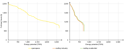
Figure 17: Full-load hours over total energy potential for solar

Table 17: Exemplary comparison of renewable potential for Germany in GW.

	Own assumption	Result for	Literature values in
	based on	current legislation	in Risch et al. (2022)
	on Auer et al. (2020)	in Risch et al. (2022)	Lowest	Highest
Wind, onshore	385.7	385.0	68.0	1188.0
Wind, offshore	83.6	79.1	34.1	99.6
PV, openspace	301.0	456.1	90.0	1285.0
PV, rooftop	177.1	492.0	43.0	746.0

The available energy potential for biomass amounts to 1,081 TWh building on Institute for Energy and Transport (2015) (Joint Research Center) and assuming 206 TWh of the total potential are used for the decarbonization of feedstock in the chemical industry instead of the modeled energy system Bazzanella and Ausfelder (2017).

Appendix E Technology data for system model

The tables here list the technology data for electricity generation in the system model from Danish Energy Agency (2022). For hydrogen fuelled plants, we assume a 15% mark-up on the costs of the corresponding natural gas plant in line with Öberg et al. (2022). This assumption neglects the cheaper alternative of retrofitting pre-existing gas plants instead. For all technologies we assume a uniform interest rate of 5%.

Table 18: Technology data for electricity generation in system model.

technology	investment costs [m€/GWin]	operational costs [m€/GWin/a]	lifetime [a]	electrical efficiency	availability
combined cycle gas turbine, backpressure turbine	586.0	13.7	25	50.3%	93.0%
combined cycle gas turbine, extraction turbine	480.7	15.9	25	58.3%	93.0%
combined cycle H2 turbine, backpressure turbine	673.9	13.7	25	50.3%	93.0%
combined cycle H2 turbine, extraction turbine	552.8	15.9	25	58.3%	93.0%
open cycle gas turbine	177.8	3.2	25	41.5%	97.2%
open cycle gas turbine CHP	226.6	7.7	25	41.5%	93.0%
open cycle H2 turbine	204.4	3.2	25	41.5%	97.2%
open cycle H2 turbine CHP	260.6	7.7	25	41.5%	93.0%
engine, biogas	384.8	3.9	25	43.3%	95.1%
engine, diesel	118.8	2.9	25	35.0%	96.8%
engine, gas	221.5	2.9	25	47.6%	98.7%
engine CHP, gas	415.5	4.2	25	46.9%	95.5%
non-solid biomass plant CHP	272.4	9.7	25	28.1%	91.2%
solid biomass plant CHP	870.5	24.9	25	26.8%	91.2%
polymer electrolyte fuel cell	475.0	23.8	10	50.0%	99.7%
solid oxide fuel cell	840.0	42.0	20	59.6%	100.0%
PV, openspace	271.2	5.4	18
PV, rooftop residential	693.8	9.5	40
PV, rooftop industry	511.7	7.8	40
wind, onshore	963.1	11.3	30
wind, offshore, shallow water	1,577.6	32.5	30
wind, offshore, deep water	1,777.3	32.5	30

Table 18: (continued)

The energy-to-power ratios for both battery technologies are constrained to be between 0.1 and 10.

Table 19: Technology data for electricity storage in system model.

			investment costs		operational costs
technology	cycle efficiency	lifetime	power capacity	energy capacity	power capacity	energy capacity
		[a]	[m€/GW]	[m€/GWh]	[m€/GW/a]	[m€/GWh/a]
lithium battery	0.89	18	80.9	199.6	1.21	2.99
redox battery	0.52	18	614	174.5	9.21	2.62
pumped storage	0.81	-	-	-	-	-

Appendix F Supply and demand time-series

Figs. 18 and 19 show hourly electricity supply and demand for an exemplary February week in Germany. The intention of these figures is to retrace the duration curves presetented in Fig. 7 of the paper. In contrast to the 52% nuclear system, Fig. 19 shows how demand adapts to supply greatly reducing the residual demand to be met by thermal plants.

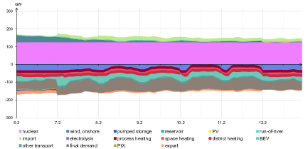
Figure 18: Supply and demand in Germany for one week and the 52% nuclear system

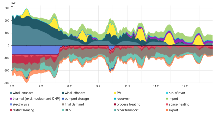
Figure 19: Supply and demand in Germany for one week and the system without nuclear

Appendix G Final demand

The table below lists the final demand for energy and transport services the system model must meet in each case.

Table 20: Final demand for different energy carriers in the energy system model.

			process heat [TWh]			passenger transport [Gpkm]			freight transport [Gpkm]
country	electricity [TWh]	space heat [TWh]	low (until 100°C)	medium (100 to 500°C)	high (above 500°C)	rail	road private	road public	rail	road heavy	road light	jet fuel [TWh]
Albania	4.6	4.2	2.7	3.8	4.9	0.1	8.6	3.0	2.5	3.8	0.0	0.0
Austria	62.8	45.2	17.0	26.2	20.7	14.0	83.8	11.0	12.6	25.6	0.9	18.1
Bosnia and Herzegovina	9.6	4.9	3.2	4.5	5.7	0.1	11.5	4.0	3.4	5.1	0.1	0.0
Belgium	73.6	62.5	17.1	22.6	28.8	11.7	117.8	14.9	5.7	30.9	3.9	51.7
Bulgaria	29.2	11.0	9.1	4.7	4.8	1.4	55.9	7.8	7.1	20.2	0.3	5.4
Switzerland	51.8	43.7	7.4	30.8	6.6	20.8	80.6	6.4	6.4	11.6	0.3	0.5
Czech Republic	57.8	38.9	17.5	16.7	19.0	10.0	76.5	17.7	19.2	46.6	3.8	5.0
Germany	480.7	470.9	112.1	119.0	153.0	101.7	950.7	64.8	84.8	303.3	8.6	151.0
Denmark	29.5	30.3	5.6	7.0	2.6	6.9	67.1	7.9	2.0	14.8	0.2	4.3
Estonia	7.2	5.3	1.0	1.9	0.6	0.4	11.3	2.4	4.1	4.7	0.1	0.0
Spain	241.9	62.8	25.5	57.2	54.1	31.0	370.9	35.0	11.4	213.9	3.1	6.1
Finland	65.8	30.4	27.7	42.4	8.7	4.6	67.8	8.1	11.8	28.4	0.5	16.7
France	390.3	257.8	40.4	57.1	64.6	95.3	770.4	59.2	19.5	169.3	4.8	114.2
Greece	45.3	16.0	5.2	5.9	5.9	1.2	106.0	21.0	0.6	27.0	1.2	69.5
Croatia	16.7	10.3	1.6	3.9	2.6	0.8	25.6	5.3	3.6	12.2	0.3	3.3
Hungary	37.1	36.6	7.1	4.1	6.9	6.7	55.1	16.2	14.5	35.8	1.1	6.1
Ireland	24.9	15.9	4.1	5.8	3.8	1.1	28.5	5.2	0.1	9.0	0.2	0.0
Italy	260.6	215.9	57.1	48.5	72.7	59.0	768.2	89.9	17.0	96.3	16.4	66.9
Lithuania	11.7	8.0	3.7	2.1	1.5	0.4	30.3	2.9	112.4	52.3	0.8	29.6
Luxemboourg	4.7	3.5	0.8	1.1	2.1	0.4	7.2	1.1	0.7	7.3	0.1	0.0
Latvia	6.2	7.6	1.7	3.9	1.5	0.6	15.3	2.6	46.9	14.8	0.2	0.0
Montenegro	2.8	0.9	0.5	0.7	1.1	0.1	4.1	0.1	0.9	1.4	0.0	0.0
Macedonia	5.2	3.1	1.9	2.6	3.4	0.1	7.5	2.2	2.1	3.2	0.0	0.0
Netherlands	107.7	62.8	30.0	28.1	42.5	24.5	187.4	6.8	8.7	66.7	1.6	215.6
Norway	106.6	34.0	4.8	30.7	2.6	3.6	64.6	4.2	3.9	20.7	0.6	17.0
Poland	145.1	98.0	23.6	40.8	42.5	21.8	218.7	35.6	127.9	340.0	9.0	35.1
Portugal	46.5	9.1	8.4	16.1	9.1	4.0	85.2	7.0	5.1	30.4	0.6	29.1
Romania	55.0	31.2	11.1	14.1	25.2	4.4	81.4	15.6	40.1	60.3	0.8	11.6
Serbia	32.7	11.2	6.8	9.6	12.0	0.3	28.8	10.0	8.5	12.7	0.2	0.0
Sweden	104.7	55.4	12.1	51.0	10.0	11.7	100.0	8.7	19.2	42.0	0.6	7.7
Slovenia	12.3	6.5	1.7	2.6	2.3	0.5	26.3	3.6	13.1	23.7	0.3	0.0
Slovakia	26.2	15.1	11.8	5.6	15.2	3.7	27.9	6.1	17.2	32.5	1.5	2.5
United Kingdom	256.4	271.8	46.9	68.6	42.1	69.1	670.3	36.5	16.7	153.7	7.1	143.9

Table 20: (continued)

Appendix H Energy flows

Figs. 20 and 21 provide a comprehensive overview of energy flows and conversion processes in the solved model for the 52% nuclear system and the system without nuclear. The resulting Sankey diagrams are the quantitative counterpart to the qualitative graphs in supplementary material C. Some technologies distinct in the model were merged into a single node for the graph to facilitate interpretation, for instance different types of BEVS.

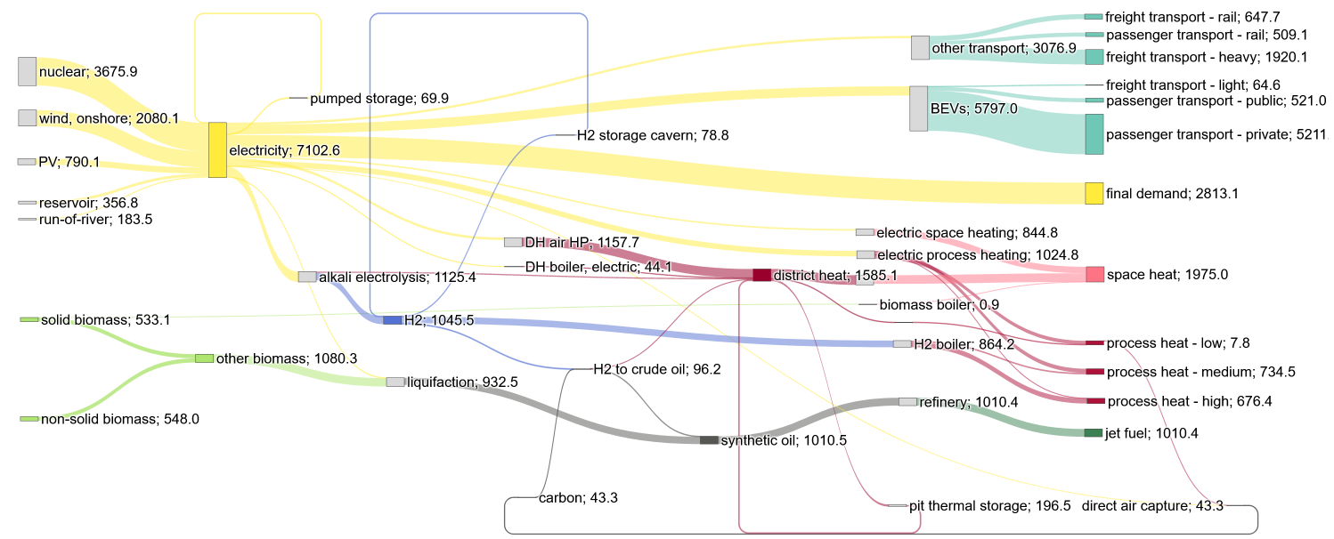
Figure 20: Sankey diagram for the 52% nuclear system, in TWh/Gpkm/Gtkm

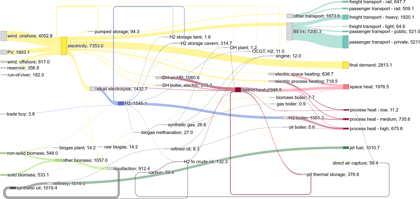
Figure 21: Sankey diagram for the system without nuclear, in TWh/Gpkm/Gtkm

References

- Financial Times (2022) Financial Times, Japan set for new nuclear plants in post-fukushima shift, August 24, 2022. URL: https://www.ft.com/content/b380cb74-7b2e-493f-be99-281bd0dd478f.
- New York Times (2022) New York Times, France announces major nuclear power buildup, February 10, 2022. URL: https://www.nytimes.com/2022/02/10/world/europe/france-macron-nuclear-power.html.
- Bloomberg (2022) Bloomberg, Uk’s nuclear gambit faces long odds even with sizewell approval, September 4, 2022. URL: https://www.bloomberg.com/news/articles/2022-09-04/uk-s-nuclear-gambit-faces-long-odds-even-with-sizewell-approval.
- Goldstein et al. (2019) J. S. Goldstein, S. A. Qvist, S. Pinker, A Bright Future: How Some Countries Have Solved Climate Change and the Rest Can Follow, Public Affairs, 2019.
- Jenkins et al. (2018) J. Jenkins, Z. Zhou, R. Ponciroli, R. Vilim, F. Ganda, F. de Sisternes, A. Botterud, The benefits of nuclear flexibility in power system operations with renewable energy, Applied Energy 222 (2018) 872–884. doi:10.1016/j.apenergy.2018.03.002.
- Lynch et al. (2022) A. Lynch, Y. Perez, S. Gabriel, G. Mathonniere, Nuclear fleet flexibility: Modeling and impacts on power systems with renewable energy, Applied Energy 314 (2022) 118903. doi:10.1016/j.apenergy.2022.118903.
- MIT (2018) MIT, The Future of Nuclear Energy in a Carbon-Constrained World, Technical Report, Massachusetts Institue of Technology, Cambridge, MA, 2018. URL: http://energy.mit.edu/wp-content/uploads/2018/09/The-Future-of-Nuclear-Energy-in-a-Carbon-Constrained-World.pdf.
- Ritchie (2022) H. Ritchie, How does the land use of different electricity sources compare?, 2022. URL: https://ourworldindata.org/land-use-per-energy-source.
- Luderer et al. (2022) G. Luderer, S. Madeddu, L. Merfort, F. Ueckerdt, M. Pehl, R. Pietzcker, M. Rottoli, F. Schreyer, N. Bauer, L. Baumstark, C. Bertram, A. Dirnaichner, F. Humpenöder, A. Levesque, A. Popp, R. Rodrigues, J. Strefler, E. Kriegler, Impact of declining renewable energy costs on electrification in low-emission scenarios, Nature Energy 7 (2022) 32–42. doi:10.1038/s41560-021-00937-z.
- Bogdanov et al. (2021) D. Bogdanov, M. Ram, A. Aghahosseini, A. Gulagi, A. S. Oyewo, M. Child, U. Caldera, K. Sadovskaia, J. Farfan, L. De Souza Noel Simas Barbosa, M. Fasihi, S. Khalili, T. Traber, C. Breyer, Low-cost renewable electricity as the key driver of the global energy transition towards sustainability, Energy 227 (2021) 120467. doi:10.1016/j.energy.2021.120467.
- Lovins (2022) A. B. Lovins, US nuclear power: Status, prospects, and climate implications, The Electricity Journal 35 (2022) 107122. URL: https://linkinghub.elsevier.com/retrieve/pii/S1040619022000483. doi:10.1016/j.tej.2022.107122.
- Rothwell (2022) G. Rothwell, Projected electricity costs in international nuclear power markets, Energy Policy 164 (2022) 112905. URL: https://linkinghub.elsevier.com/retrieve/pii/S0301421522001306. doi:10.1016/j.enpol.2022.112905.
- EDF (2022) EDF, Universal Registration Document 2021 - Including the Annual Financial Report, Technical Report, Paris, 2022. URL: https://www.edf.fr/sites/groupe/files/2022-03/edf-2021-universal-registration-document.pdf.
- Deutsche Welle (2022) Deutsche Welle, Finland’s much-delayed nuclear plant launches, March 12, 2022. URL: https://www.dw.com/en/finlands-much-delayed-nuclear-plant-launches/a-61108015.
- BBC (2022) BBC, Hinkley point c delayed by a year as cost goes up by £3bn, May 20, 2022. URL: https://www.bbc.com/news/uk-england-somerset-61519609.
- Berthélemy and Escobar Rangel (2015) M. Berthélemy, L. Escobar Rangel, Nuclear reactors’ construction costs: The role of lead-time, standardization and technological progress, Energy Policy 82 (2015) 118–130. doi:10.1016/j.enpol.2015.03.015.
- Grubler (2010) A. Grubler, The costs of the french nuclear scale-up: A case of negative learning by doing, Energy Policy 38 (2010) 5174–5188. doi:10.1016/j.enpol.2010.05.003.
- Wang et al. (2018) D. Wang, M. Muratori, J. Eichman, M. Wei, S. Saxena, C. Zhang, Quantifying the flexibility of hydrogen production systems to support large-scale renewable energy integration, Journal of Power Sources 399 (2018) 383–391. doi:10.1016/j.jpowsour.2018.07.101.
- Schill and Zerrahn (2020) W.-P. Schill, A. Zerrahn, Flexible electricity use for heating in markets with renewable energy, Applied Energy 266 (2020) 114571. doi:10.1016/j.apenergy.2020.114571.
- Schuller et al. (2015) A. Schuller, C. M. Flath, S. Gottwalt, Quantifying load flexibility of electric vehicles for renewable energy integration, Applied Energy 151 (2015) 335–344. doi:10.1016/j.apenergy.2015.04.004.
- McKenna et al. (2014) R. McKenna, S. Hollnaicher, W. Fichtner, Cost-potential curves for onshore wind energy: A high-resolution analysis for germany, Applied Energy 115 (2014) 103–115. doi:10.1016/j.apenergy.2013.10.030.
- Göke (2021) L. Göke, Anymod.jl: A julia package for creating energy system models, SoftwareX 16 (2021) 100871. doi:10.1016/j.softx.2021.100871.
- Duan et al. (2022) L. Duan, R. Petroski, L. Wood, K. Caldeira, Stylized least-cost analysis of flexible nuclear power in deeply decarbonized electricity systems considering wind and solar resources worldwide, Nature Energy (2022). doi:10.1038/s41560-022-00979-x.
- Baik et al. (2021) E. Baik, K. P. Chawla, J. D. Jenkins, C. Kolster, N. S. Patankar, A. Olson, S. M. Benson, J. Long, What is different about different net-zero carbon electricity systems?, Energy and Climate Change 2 (2021) 100046. doi:doi.org/10.1016/j.egycc.2021.100046.
- Lévêque (2014) F. Lévêque, The Economics and Uncertainties of Nuclear Power, Cambridge University Press, Cambridge, MA, USA, 2014.
- Lordan-Perret et al. (2021) R. Lordan-Perret, R. D. Sloan, R. Rosner, Decommissioning the U.S. nuclear fleet: Financial assurance, corporate structures, and bankruptcy, Energy Policy 154 (2021) 112280. URL: https://linkinghub.elsevier.com/retrieve/pii/S030142152100149X. doi:10.1016/j.enpol.2021.112280.
- Wheatley et al. (2016) S. Wheatley, B. K. Sovacool, D. Sornette, Reassessing the safety of nuclear power, Energy Research & Social Science 15 (2016) 96–100. URL: https://linkinghub.elsevier.com/retrieve/pii/S2214629615301067. doi:10.1016/j.erss.2015.12.026.
- Lehtveer and Hedenus (2015) M. Lehtveer, F. Hedenus, Nuclear power as a climate mitigation strategy – technology and proliferation risk, Journal of Risk Research 18 (2015) 273–290. URL: http://www.tandfonline.com/doi/abs/10.1080/13669877.2014.889194. doi:10.1080/13669877.2014.889194.
- Stirling (1997) A. Stirling, Limits to the value of external costs, Energy Policy 25 (1997) 517–540. URL: https://linkinghub.elsevier.com/retrieve/pii/S0301421597000414. doi:10.1016/S0301-4215(97)00041-4.
- Göke et al. (2023) L. Göke, J. Weibezahn, M. Kendziorski, How flexible electrification can integrate fluctuating renewables, 2023. URL: https://arxiv.org/abs/2301.11096.
- Haas et al. (2019) R. Haas, S. Thomas, A. Ajanovic, The Historical Development of the Costs of Nuclear Power, in: R. Haas, L. Mez, A. Ajanovic (Eds.), The Technological and Economic Future of Nuclear Power, Springer VS, Wiesbaden, 2019, pp. 97–116. URL: http://link.springer.com/10.1007/978-3-658-25987-7_12. doi:10.1007/978-3-658-25987-7_12.
- MacKerron (1992) G. MacKerron, Nuclear costs: Why do they keep rising?, Energy Policy 20 (1992) 641–652. URL: https://linkinghub.elsevier.com/retrieve/pii/030142159290006N. doi:10.1016/0301-4215(92)90006-N.
- NREL (2021) NREL, 2021 Annual Technology Baseline, Technical Report, National Renewable Energy Laboratory, Golden, CO, 2021. URL: https://atb.nrel.gov/electricity/2021/data.
- OECD and NEA (2018) OECD, NEA, The Full Costs of Electricity Provision, Technical Report NEA No. 7298, Nuclear Energy Agency, Boulogne-Billancourt, France, 2018. URL: https://www.oecd.org/publications/the-full-costs-of-electricity-provision-9789264303119-en.htm.
- Shirvan (2022) K. Shirvan, Overnight Capital Cost of the Next AP1000, Technical Report MIT-ANP-TR-193, Massachusetts Institue of Technology, Cambridge, MA, 2022.