Intergenerational Mobility Trends and the Changing Role of Female Labor

Abstract

Using harmonized administrative data from Scandinavia, we find that intergenerational rank associations in income have increased uniformly across Sweden, Denmark, and Norway for cohorts born between 1951 and 1979. Splitting these trends by gender, we find that father-son mobility has been stable, while family correlations for mothers and daughters trend upward. Similar patterns appear in US survey data, albeit with slightly different timing. Finally, based on evidence from records on occupations and educational attainments, we argue that the observed decline in intergenerational mobility is consistent with female skills becoming increasingly valued in the labor market.

Keywords— Intergenerational Mobility, Labor Force Participation JEL— J62, J21

1 Introduction

A central question in the social sciences is the intergenerational transmission of human capital. Empirical studies of the influence of family environment often estimate the relationship between the income of parents and their children. Early work by for instance Becker and Tomes (1979) and Solon (1999) highlights that in such estimations, it is essential to account for the role of idiosyncratic labor market conditions. Accordingly, variation in labor market conditions may shape estimates of intergenerational mobility across space (Solon, 2002; Chetty et al., 2014a; Bratberg et al., 2017) and time (Corak, 2013). While substantial time-variation in mobility has been documented (see e.g. Lee and Solon, 2009; Olivetti and Paserman, 2015; Chetty et al., 2014b), little is known about how changes in labor market conditions shape these patterns (see e.g. Song et al., 2020, for a notable exception).

In this paper, we ask what implications the “grand convergence” between men and women in labor market conditions (Goldin, 2014) has had for intergenerational income mobility. Measuring inherent (“latent”) human capital among women has been difficult historically for at least three reasons: we don’t observe income for non-workers, selection into market work has made the average skills among working women unrepresentative of the population average (Blau et al., 2021), and discrimination against female workers has hindered correct measurement of their true latent skills. These factors introduce measurement error in female income, which attenuates estimates of mother-child and father-daughter income mobility. Over the past 50 years, women in all Western economies have become more likely to participate in market work (Olivetti and Petrongolo, 2016) and occupational segregation of men and women has decreased (Blau, Brummund and Liu, 2013) — changes which should gradually lessen the degree of bias in mobility estimates.

We address the question of how changes in female labor supply affect intergenerational mobility by turning to the three Scandinavian countries. The high quality of Scandinavian administrative data allows us to follow how the changing patterns in female labor supply affect earnings at the individual level. In turn, this enables studying how mother-child and father-child transmission of human capital, respectively, has evolved over time. Scandinavia provides an ideal setting for understanding how the changing labor supply of women might affect intergenerational mobility, as the development toward gender equality precedes that in other countries (Kleven, Landais and Søgaard, 2019). We document trends in intergenerational mobility in Sweden, Denmark, and Norway for cohorts of children born between 1951 and 1979, using administrative income data from 1968 up until 2017. By applying a unified approach to long panels of full-population administrative data for three countries, we can ensure that any differences in findings are not related to country-specific developments, the choice of data period, or the income definition.

Our results reveal a substantial decline in intergenerational income mobility in Scandinavia that remains robust across a large set of common empirical specifications. However, this decline is only present among mother-child and father-daughter pairs. In the earliest cohorts in our analysis, child earnings — in particular earnings of sons — were virtually uncorrelated with the earnings of mothers, while exhibiting a clear and economically significant correlation with the earnings of fathers. Over time, these parent-specific mobility estimates between children and their mothers and fathers, respectively, have all converged to similar levels. We further show that this is not solely an effect of extensive margin labor supply increasing among women, but also stems from women entering more skilled occupations. In fact, most of the change in mobility estimates takes place during a time period where maternal labor force participation is already high, but where the occupational composition of mothers is changing rapidly.

Conducting a similar analysis on Panel Study of Income Dynamics (PSID) data from the US, we find comparable patterns in mother-child and father-child income persistence, albeit with a slightly lagged timing. Despite its small sample size by birth cohorts (averaging 150 parent-child pairs) (Davis and Mazumder, 2022), the PSID is regularly used to study parent-child income persistence (Justman, Krush and Millo, 2017; Hertz, 2008; Hartley, Lamarche and Ziliak, 2022). See Mazumder (2018) for an overview of the PSID in research on intergenerational mobility. It enables us to extend our results to the US and provide suggestive evidence that the observed patterns are not solely a Scandinavian phenomenon.

Next, we set up a simple model of gender-specific mobility and latent productivity, inspired by some of the building blocks in the model by Becker and Tomes (1979). We decompose the trend in intergenerational mobility into parts that reflect assortative mating (correlations in parental skills), gender-neutral skills transmission, gender-specific skills transmission, and gender-specific return on skill. Calibrating the model to country-specific aggregate data for cohorts of children born from 1962 to 1979, we show that the observational downward trend in intergenerational mobility is largely compatible with increasing returns to inheritable skills among women, relative to men. The decomposition thus suggests that the observed trends in income mobility are artifacts of changes in how women participate in the labor market.

In the final part of the paper, we corroborate the decomposition exercise empirically, by showing that gender-specific intergenerational correlations in economic status — measured by combining own income, years of education, and occupation using the proxy variable index suggested by Lubotsky and Wittenberg (2006) — remain constant over time, or are only weakly increasing. Mobility also remains at a constant level when correlating son earnings with those of their maternal uncles, as another way to proxy for maternal skills. Our evidence is consistent with that the observed trends in intergenerational income mobility can be explained by income rank correlations between children and parents gradually becoming less attenuated by frictions caused by gender segregation in the labor market. Intergenerational mobility in income did in fact decline consistently in Scandinavia across cohorts born between 1951 and 1979, but this was driven by female earnings becoming more reflective of their actual skills. The return on latent productivity of women has converged towards that of men. The observed development in intergenerational mobility can therefore potentially be seen as a natural implication of a socially desirable development, rather than a sign of actually declining equality of opportunity.

The literature on trends in intergenerational mobility includes results from a wide range of settings and empirical specifications, all of which affect conclusions on the existence and direction of the trends (Engzell and Mood, 2023). Trend estimates focusing on similar birth cohorts as those included in our study generally find increasing levels of income persistence, including evidence from Canada (Connolly, Haeck and Lapierre, 2019), the US (Jácome, Kuziemko and Naidu, 2021; Davis and Mazumder, 2022), the UK (Blanden et al., 2004), Sweden (Brandén and Nybom, 2019; Engzell and Mood, 2023), Norway (Markussen and Røed, 2020) and Denmark (Harding and Munk, 2019).

Recent studies have proposed several explanations for downward trends in mobility, none of which are consolidated across countries and specifications. Davis and Mazumder (2022) suggest that the return to education has increased, which, given that education and human capital are significant channels for the transmission of income across generations, has led to a decline in mobility. A similar explanation put forward by Connolly, Haeck and Laliberté (2020) is that the degree to which women obtain secondary education has increased. Observing that conditional on parental income, income in the child generation is “boosted” by a higher level of education among parents, the authors conclude that this upward trend in mothers’ level of education must have led to a decline in social mobility. However, the underlying mechanism of this relationship remains unclear. Harding and Munk (2019) suggest other explanations, such as changes in family structure including marital status, assortative mating, and childbearing among women.

A noteworthy strand in the mobility literature has previously highlighted that cross-sectional estimates of intergenerational mobility may differ substantially by gender due to different opportunities for men and women in the labor market (Corak, 2013; Lee and Solon, 2009). Studies on gender and trends in intergenerational mobility mainly differentiate between sons and daughters. One set of recent studies finds that mobility decreased for children of both sexes (Blanden et al., 2004; Connolly, Haeck and Lapierre, 2019). Harding and Munk (2019) find sharply increasing parent-daughter and parent-son correlations for Danish cohorts born between 1957 and 1977. Conversely, studying cohorts born between the 50s and the 70s in Finland, Pekkala and Lucas (2007) find declining levels of mobility for daughters, but stable trend estimates for sons — results that are echoed for Norway in Markussen and Røed (2020) and Pekkarinen, Salvanes and Sarvimäki (2017). Patterns by gender of both parents and children have previously been documented, though not extensively discussed, in Brandén and Nybom (2019); Engzell and Mood (2023) and Jácome, Kuziemko and Naidu (2021).

With this paper, we make two contributions to the understanding of time variation in intergenerational mobility. First, we provide clear evidence of a uniform decline in intergenerational income mobility across Scandinavia for cohorts born between 1951 and 1979. We show that this trend holds irrespective of methodological choices and does not stem from country-specific policies, therefore corroborating results in Harding and Munk (2019); Pekkarinen, Salvanes and Sarvimäki (2017); Brandén and Nybom (2019) and Markussen and Røed (2020). Further, we extend this cross-country comparison to gender-specific trends of mothers, fathers, sons, and daughters, and provide evidence of a similar pattern in the US from panels of linked survey data. The findings suggest that not only do mobility levels vary by gender Chadwick and Solon (2002); Lee and Solon (2009); Corak (2013), but secular changes in gender-specific earnings determinants have also caused trends to differ substantially, in turn causing levels to converge.

The second, and main, contribution of this paper is to show that the decline in mobility can be fully (Sweden, Norway) or mostly (Denmark) accounted for by changing female labor force participation. While previous studies have concluded that mother-child correlations are the driving force behind declining mobility (Engzell and Mood, 2023), we are the first to explicitly show that this is happening because of the changing role of women in market labor. We show a connection between declining overall mobility estimates and female participation in the labor market, including the valuation of female skills. In other words, female labor market conditions have caused parental earnings to be substantially better reflected in child earnings — hence inducing a real downward shift in intergenerational mobility — in spite of the between-generation correlation in latent skills being relatively constant.

The remainder of the paper is structured as follows. Section 2 provides a brief overview of the key features of the Scandinavian welfare states, and Section 3 describes our data sources. In Section 4 we describe the common methodology used to estimate intergenerational income mobility and present our main results. Section 5 builds and calibrates a model for the connection between intergenerational rank associations and increasing female labor force attachment. In Section 6, we show how the estimated trends change when we use a measure of maternal economic status that better captures female earnings potential. Section 7 concludes.

2 Institutional Context

The Scandinavian countries share similar traits in terms of economic development, political culture, and institutions. The welfare states are of universal character, with access to social security benefits, health care, subsidized childcare, and tuition-free higher education (Baldacchinoel and Wivel, 2020). In order to finance the provision of these public goods, marginal tax rates at the top of the income distribution and the average tax burden are substantially higher in Scandinavia than in other developed countries (Kleven, 2014). Employees are to a large degree organized in unions and wages are often collectively bargained (Pareliussen et al., 2018). Historically, all three countries have been characterized by low levels of inequality and high levels of income mobility, in comparison to other Western countries (Søgaard, 2018; Bratberg et al., 2017).

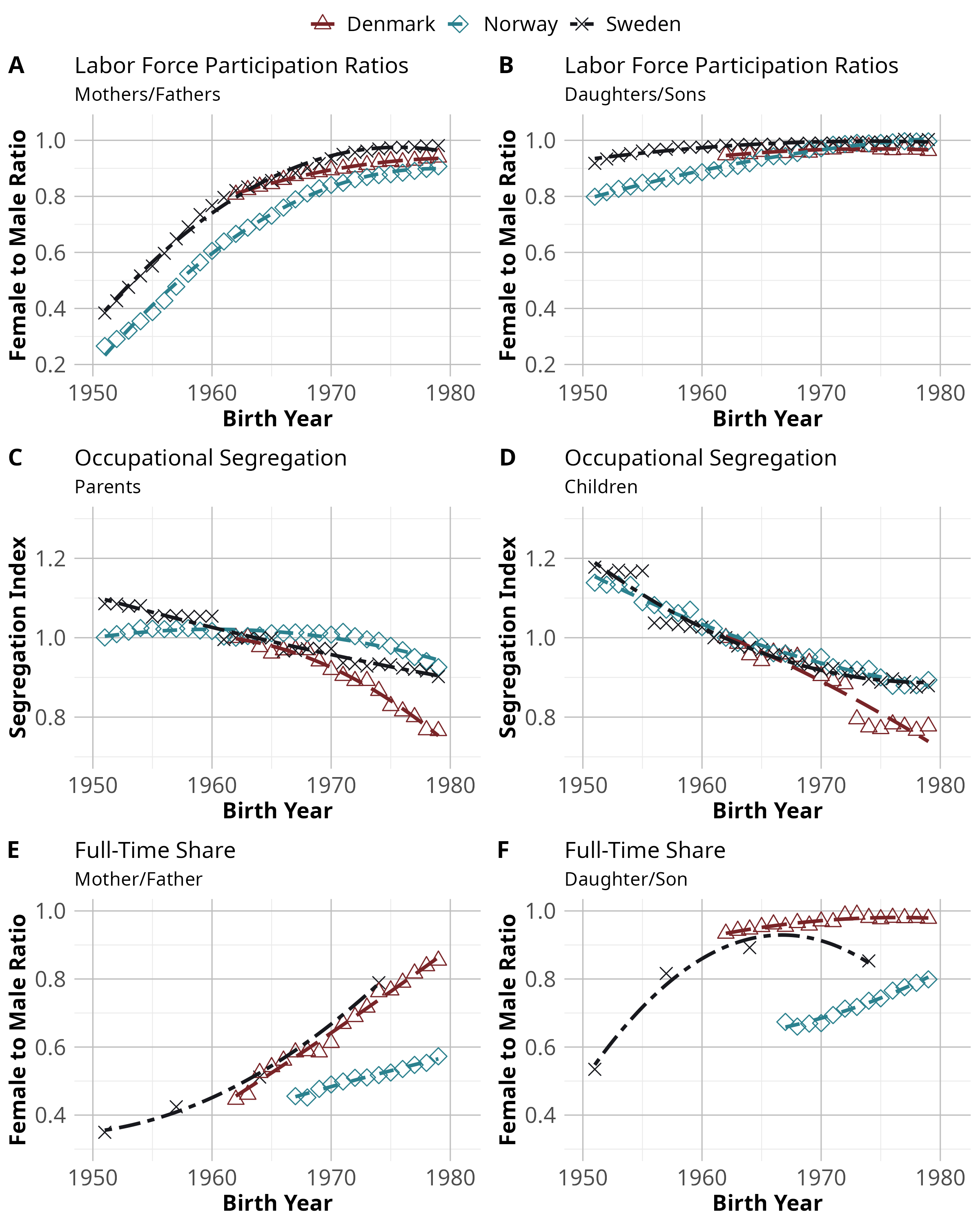
Figure 1: Changes in Gender Differences in Labor Force Participation, Occupational Segregation and Working Hours.

Notes: Panel A and B depict female-to-male ratios of labor force participation in our main samples; for parents in Panel A and for children in Panel B. The labor force participation rate is based on annual labor earnings: a person is considered in the labor force if they have annual earnings exceeding the equivalent of 10,000 USD (2017). Panels C and D depict an index for labor market segregation, for parents and children respectively. The index is normalized to the base year 1962. In some years, Danish occupational codes have been imputed from other variables — therefore, the Danish trend in occupational segregation should be interpreted with caution (see more in Appendix A). Panels E and F provide female-to-male ratios of full-time work. Full-time work is defined as working at least 27 hours in Denmark and Sweden, and at least 31 hours in Norway. Data for full-time shares is obtained from linked employer-employee data in Norway and Denmark, and nationally representative surveys in Sweden. In Denmark, there is a significant data break in the full-time definition which only affects the child cohort — we attempt to adjust for this appropriately with a simple correction procedure (see more in Appendix A). “Birth Year” refers to the birth year of the child in each parent-child pair.

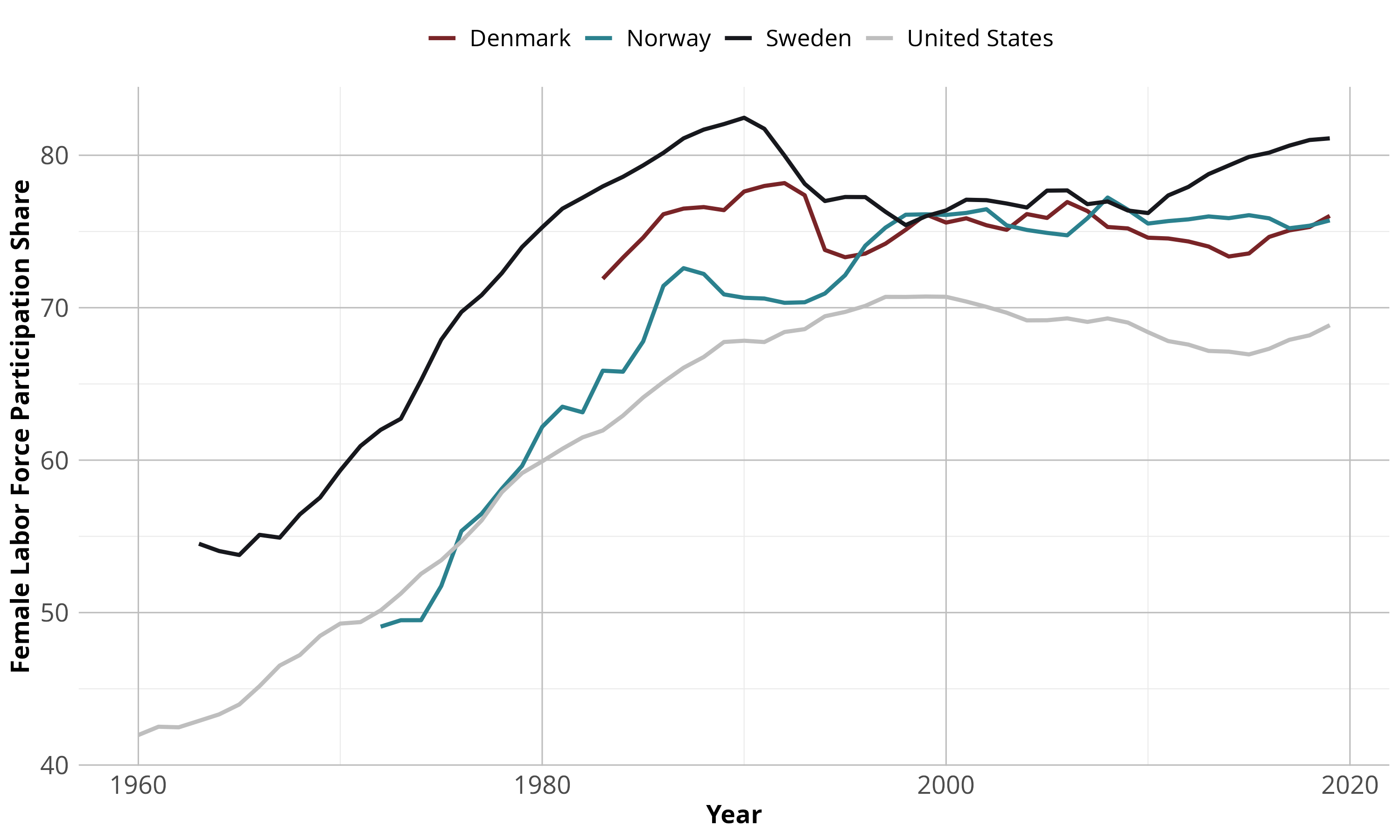
Figure B1: Female Labor Force Participation Rate.

During the second half of the 20th century, the role of women in society, and particularly in the labor market, experienced a “grand convergence” towards the position of men (Goldin, 2014). The individualization of the tax system (Selin, 2014), the introduction and expansion of paid paternity leave (Ruhm, 1998), and the expansion of compulsory and higher education (Meghir and Palme, 2005; Black, Devereux and Salvanes, 2005) all contributed to this development. As a result, female labor force participation increased from the early 1950s and is currently higher in Scandinavia than in most other Western economies (see Appendix Figure B1 for a comparison between Scandinavia and the United States).

In Figure 1 we provide some descriptive evidence on the development of female labor, for the parent and child generations separately. Panels A and B show how labor force participation among women converged to the male level. Participation rates of mothers with children born in the 1950s were less than half the rate of fathers, but this gap had closed almost entirely for mothers of children born in the 1970s. It is even less pronounced when we compare sons and daughters of a given birth year.

Panels C and D show the development of occupational segregation, i.e. the extent to which men and women work in the same occupations. The segregation index is calculated as the difference in the share of all women and men in the labor force who work in a given occupation, summed over all observed occupations (Duncan and Duncan, 1955). To make comparisons of trends easier, we normalize the index with 1962 as the base year, allowing for an interpretation of occupational segregation relative to the 1962 level. Evidently, occupational segregation has declined persistently over time, similar to the development in the United States, as documented by Blau, Brummund and Liu (2013) and Blau and Kahn (2017). In contrast to the development of female labor force participation, the decline in occupational segregation is to a larger extent present in the child generation, rather than the parent generation.

In addition, the intensive margin labor supply of women increased during the time period under study. Panels E and F provide female-to-male ratios of the share of individuals working full-time, by birth year of the child. For Denmark and Sweden, full-time work is defined as at least 27 working hours per week, while full-time in the Norwegian data is defined as at least 31 weekly hours. In Panel E, we present this for mothers relative to fathers. Similar to the development in labor force participation, mothers have continuously caught up to the rate at which fathers work full time, although a sizable difference remains toward the end of our sample period. The level differences between Sweden/Denmark and Norway stem from different full-time definitions in the data. Moreover, the convergence in intensive margin labor supply in all countries is almost entirely driven by increases in female full-time shares; male full-time shares are almost constant over the entire time period under study. Especially in Norway, our data reveals a significant remaining gender gap in hours worked. Notably, the Swedish female-to-male full-time ratio has increased at a higher rate since around 1960. The full-time ratio of daughters compared to sons, in Panel F, shows two conflicting observations. On the one hand, looking at Sweden and Denmark, the female full-time rate in the 1960s cohort was already quite high, with only small changes after that. On the other hand, the Norwegian series, using a stricter definition, suggests that a significant gender gap in working hours persists also among the child generation of our sample.

Overall, the three labor market measures presented in Figure 1 show a substantial gender convergence in labor market participation. Convergence in extensive margin labor force participation of mothers happened faster before the 1960s birth cohort, and was almost entirely equal to the fathers’ level for the 1979 cohort. Changes in occupational choice and intensive margin labor supply of mothers were, however, more predominant in the second part of our sample, after the 1960 cohort, compared to those born before 1960. We will later argue that both the extensive and intensive margin developments in labor market participation have key implications for our measures of trends in intergenerational mobility.

3 Data

For our main analysis, we use register data from Denmark, Norway, and Sweden that cover the whole population of each country. This is available from 1968 to 2017 for Norway and Sweden and from 1980 to 2017 for Denmark. The data consist of linked administrative records that provide a variety of information, including birth year, educational attainment, earnings and other income measures, family status, and various demographic variables. Individuals can be linked to their parents, which allows us to create data sets containing all child-parent pairs in a given time frame, with relevant individual income measures. For more details about the registers used, see Appendix A.

Our Scandinavian estimation sample consists of all children born between 1951 (1962 for Denmark) and 1979, who (i) have a valid personal identifier, and (ii) have at least one parent with a valid identifier. As this means that we remove a significant share of immigrants from our samples — in particular in early years — we remove all foreign-born individuals and all children with foreign-born parents. Sample sizes per birth year are approximately 70,000 child-parent pairs in Denmark, 60,000 pairs in Norway, and 100,000 pairs in Sweden, with variation over time.

Moreover, we look at parent-child income correlations in the US using data from the Panel Study of Income Dynamics (PSID). The PSID is a nationally representative survey that covers information on employment, income, occupation, education, and family links, starting from 1968. The PSID follows families and individuals across time and has a relatively low attrition rate. With this data, we create a sample of child-parent pairs for the US in a comparable, yet more limited, fashion than our analysis on the main Scandinavian samples. In total, the US sample contains about 5,000 child-parent pairs.

The PSID offers a nationally representative sample from the Survey Research Center (SRC) as well as a non-representative sample that predominantly comprises low-income families, known as the Survey of Economic Opportunities (SEO). Our primary dataset merges information from both these sources. However, we present supplementary evidence in the Appendix that supports the trends observed in the SRC sample alone, though with slightly broader confidence intervals. Despite its utility, the PSID does have constraints in estimating intergenerational mobility trends (Mazumder, 2018). Consequently, we place a greater emphasis on the comprehensive results sourced from the higher-quality Scandinavian administrative data.

The main income specifications are chosen for easy comparisons with much of the recent literature (see e.g. Chetty et al. (2014a) and Lee and Solon (2009)). Income for the child generation is defined as three-year averages of annual labor income. See Appendix Table A for an overview of the earnings components and how these compare across countries. This is measured at ages 35-37, which balances the need for a measure of permanent income rank with the need for measuring child incomes relatively early in order to maximize the number of cohorts that can be included in the analysis (Nybom and Stuhler, 2016; Bhuller, Mogstad and Salvanes, 2017).

Parental income is defined as the average of maternal and paternal individual income, measured as three-year averages of annual labor earnings around age 18 of the child. In general, this means measuring the parents’ income at age 40 or later, which is considered a meaningful proxy for lifetime income in the literature (Nybom and Stuhler, 2016). In our Appendix, we provide robustness checks to different income definitions for child and parent income variables, such as estimating trends in total factor (gross) income or net-of-tax income and evaluating the sensitivity to the exact age at which we measure child income. Finally, due to the fact that we measure parent income at age 18 of the child. The estimated trends are not sensitive to this choice, but it allows us to include younger cohorts as compared to a parental income measure captured at age 35 of the parent. Ranking parent income within birth year of both the child and the parent jointly, we are able to verify that the observed mobility trends are not driven by this measurement issue.

4 Trends in Intergenerational Mobility

In this section, we first describe the empirical method we apply for measuring child-parent rank associations, and present the trend for Scandinavia. We then analyze rank associations when we split the sample into sons, daughters, mothers, and fathers, and compare our Scandinavian results to suggestive US estimates. Finally, we discuss to what extent this trend can be attributed to changes in the intensive- or extensive-margin labor supply of women.

4.1 Empirical Method

In order to measure intergenerational income persistence, we transform observed income into cohort-specific ranks, as in Dahl and DeLeire (2008) and Chetty et al. (2014a). Using ranks, rather than levels or logs, offers certain advantages in this context. First, estimated rank correlations have proven to be less prone to life-cycle bias than other measures (Nybom and Stuhler, 2017), and in addition, the use of ranks enables the inclusion of zero incomes. However, in order to ensure that our results are not driven by the rank transformation, we also present mobility trends in intergenerational income elasticities (IGE) in the Appendix.

Rank correlations are estimated with the following regression, separately by birth cohort and country:

$$\text{Rank}_{it}^{\text{C}}=\alpha_{t}+\beta_{t}\text{Rank}_{it}^{\text{P}}+\varepsilon_{it},\qquad\forall\quad t\in\left[1951,1979\right],$$ (1)

where $\text{Rank}_{it}^{\text{C}}$ is the percentile rank of child $i$’s average income at age 35-37 within the distribution of all children born in year $t$. When we analyze sons and daughters separately, we calculate their income rank separately by gender. $\text{Rank}_{it}^{\text{P}}$ is the percentile rank of the same child’s parents’ income within the distribution of all parents with children in birth cohort $t$, averaged over ages 17-19 of the child. The coefficient $\beta_{t}$ captures the average cohort-specific parent-child correlation in income ranks, sometimes referred to as the intergenerational rank association (IRA). Lower values of $\beta_{t}$ are interpreted as lower rank associations in income, and thus higher levels of intergenerational mobility.

For the primary analysis, we rank individuals within their respective birth cohorts. In scenarios where parents are assessed, we rank them in accordance with their child’s birth cohort. Notably, when delineating income based on the gender of either the parents or offspring, we prioritize re-ranking. This procedure provides us with full support in our ranks for all specifications, given the notably lower income levels for mothers in the earliest cohorts.

Intuitively, one can think of the IRA as the correlation in inheritable skills and values that are transmitted across generations. These are attenuated by earnings determinants that cannot be passed on to children, which reduces the signal value of parental income. Such ”noise” may stem from individual-specific idiosyncratic shocks to the earnings process or time-specific characteristics of the labor market. In particular, changes in the IRA over time are not necessarily driven by transmissible factors, but rather by the importance of earnings determinants that cannot be passed on to children. In the context of analyzing how changing female labor market participation may have affected the intergenerational association in income, this is a relevant consideration.

4.2 Estimated Trends

In Figure 2, we present estimates for country-specific trends in intergenerational rank associations in individual labor income. Each point in the graph represents a slope parameter for a cohort-specific regression of equation (1) with linear trends estimated separately for 1951-1961 and 1962-1979. We provide fitted lines separately to facilitate comparisons between Denmark, Norway, and Sweden for the cohorts where all countries have available data. Appendix Table B3 provides an overview of the IRA coefficients for different specifications and tests whether trends are statistically different across countries.

From Figure 2, it appears that intergenerational mobility, measured using the IRA, has declined in all three countries, with the fastest rate of decline in Denmark. There, the rank association in income increased by 7.5 rank points (39%) from 1962 to 1979 — equivalent to an average annual increase of 0.44 rank points. While smaller than in Denmark, the trends in Norway and Sweden are by no means negligible. From 1962 to 1979, the rank association in income increased by 6.4 and 4.4 rank points (38% vs. 25%) in Norway and Sweden, respectively, yielding annual increases of 0.38 and 0.25. From 1951 to 1979, the total change in IRA for Norway is 7.8 rank points (50%) and 5.8 rank points for Sweden (34%).

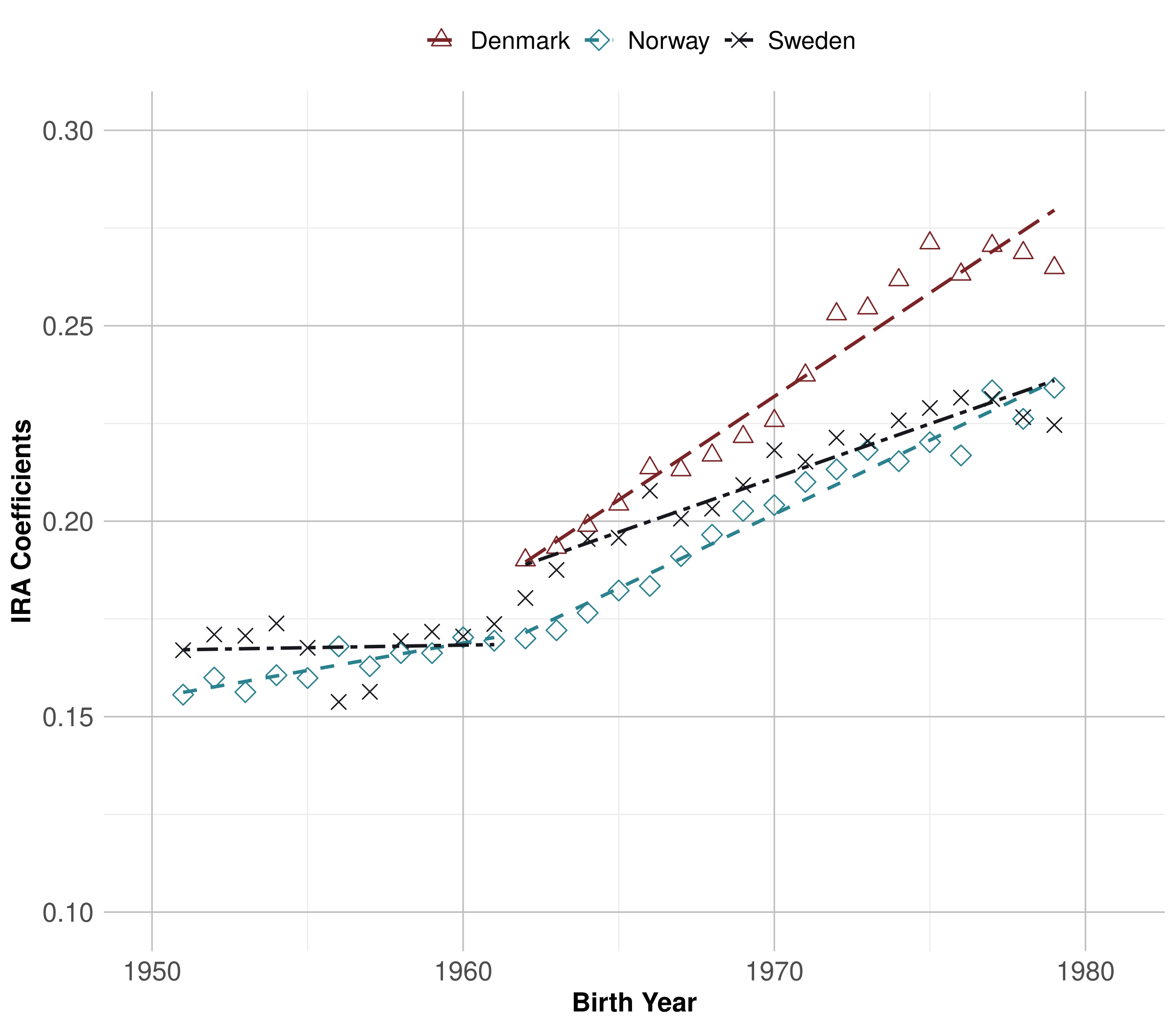
Figure 2: Trends in Intergenerational Mobility in Individual Labor Income.

Notes: The figure plots the coefficients for the intergenerational rank association (eq. 1) in individual labor income for Sweden, Denmark and Norway for birth cohorts 1951 (1962) to 1979. “Birth Year” refers to birth year of the child in each parent-child pair. Each panel shows fitted trend lines separately for the period 1951 to 1962 and 1962 to 1979.

One may wonder what it actually means, in economic terms, that the rank association in income increased by up to 0.44 rank points per year in Scandinavia. Abstracting from nonlinearities in the relationship between parent and child income ranks, a straightforward interpretation is the following: for two children born by parents in the bottom versus the top percentile, the difference in the conditional expectation of their income ranks as adults increased by 0.44 each year — amounting to as much as 4.4 rank points over a decade. Taking the Norwegian results as an example, another interpretation of the observed trends is that in the earliest observed birth cohort, a ten rank points difference in parental income corresponded to an average difference in income ranks of 1.6 between their children. In contrast, the same difference was 2.3 rank points for children born in the latest cohort. While still indicating relatively high levels of mobility by international standards, such changes over relatively short periods of time are by all means economically substantial.

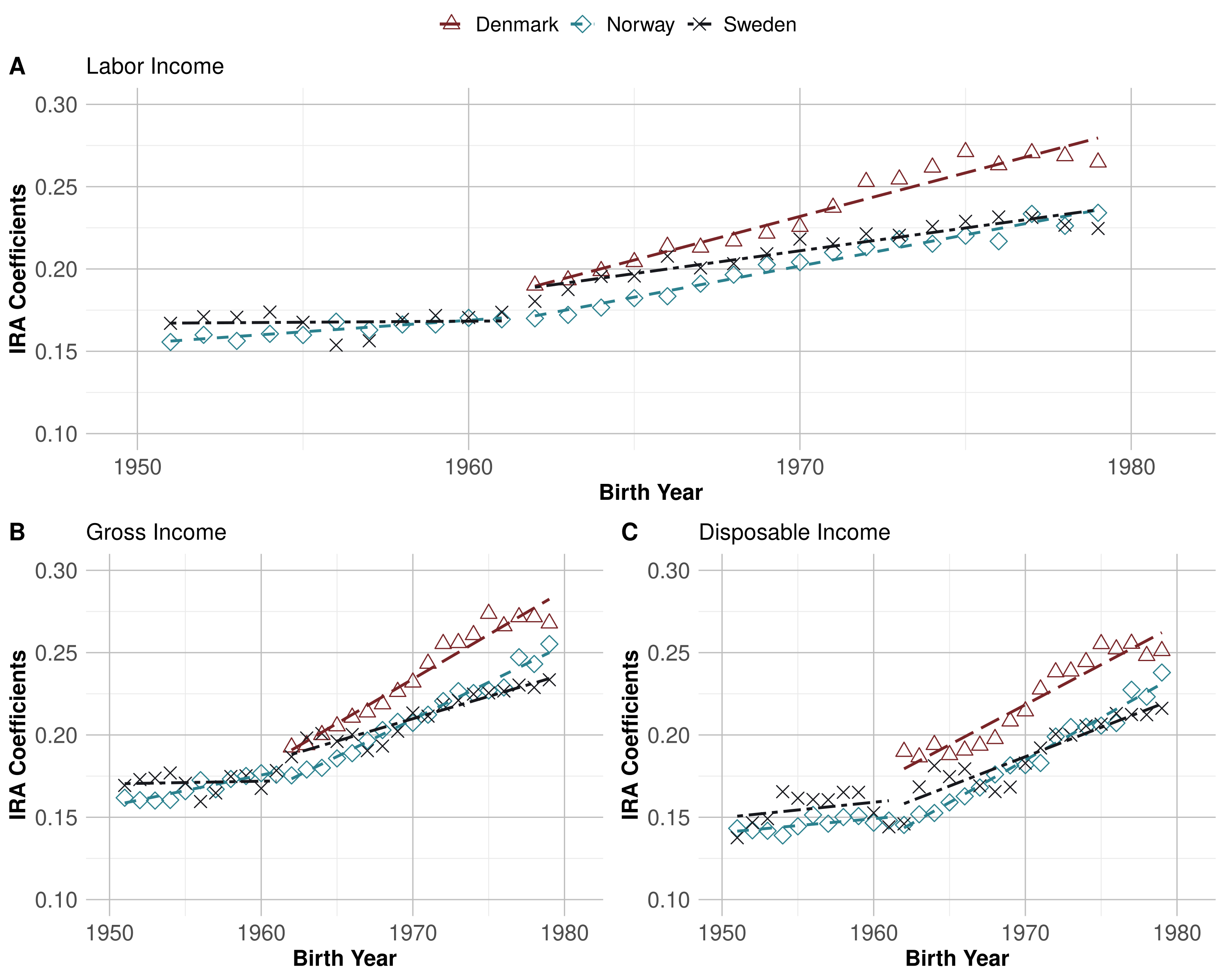
Figure B3: Estimates of IRA in Labor, Net-of-tax and Gross Income.

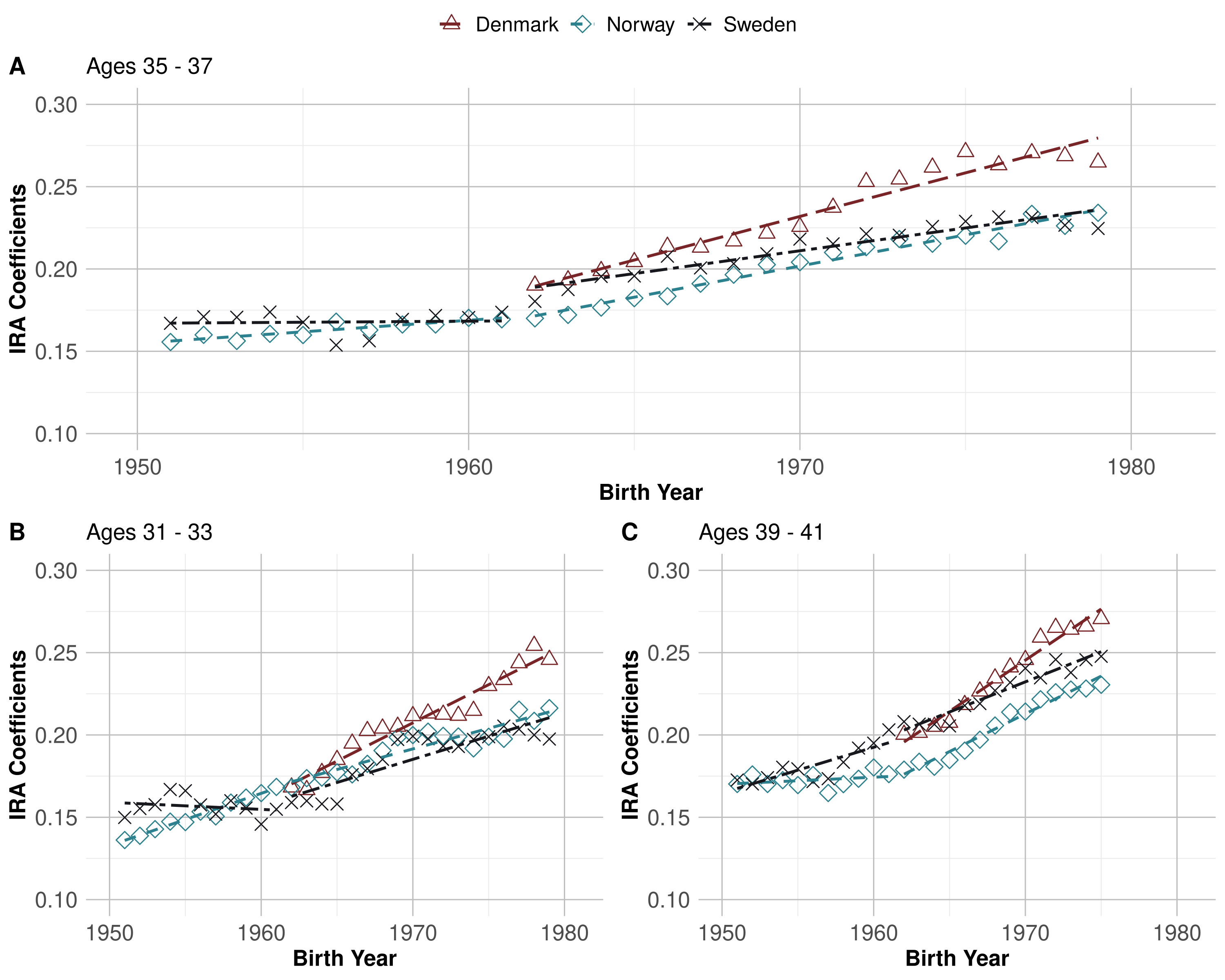
Figure B4: Estimates of IRA at Different Ages of the Child (Labor Income).

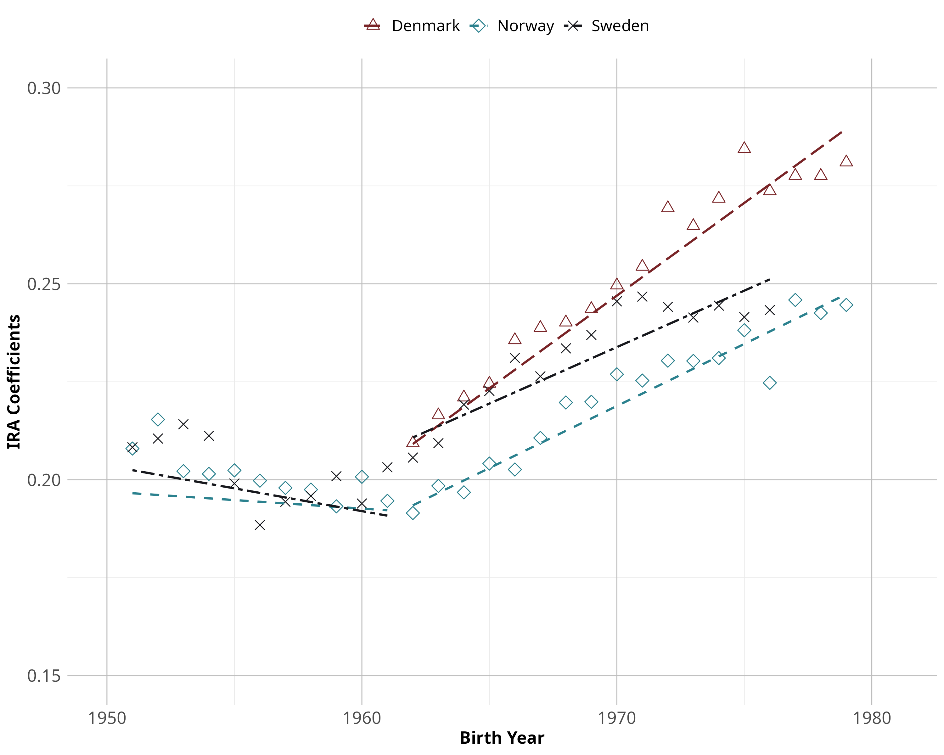
Figure B5: Estimates of IRA using Household Income in Parent and Child Generation.

In order to ensure that the trends are robust and reflect structural changes in the economy (as opposed to being something that purely exists within a narrow set of specifications), we document similar trends for a large set of different specifications in Appendix B. Most importantly, we show that the trends remain largely similar when measured in net-of-tax- and gross income (Figure B3), when measuring child income at various ages (Figure B4), and when using a measure of household income following Chetty et al. (2014a) (Figure B5).

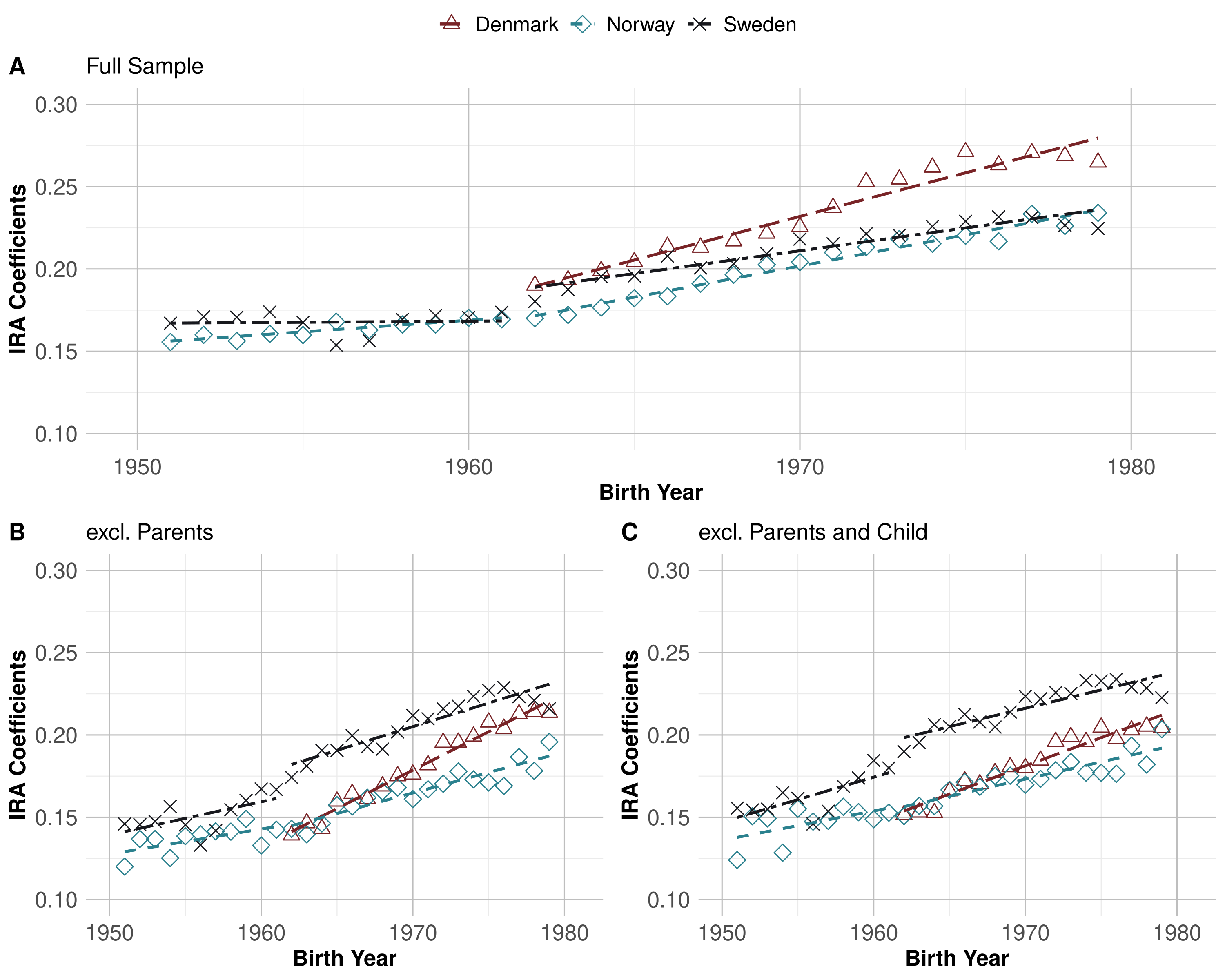
Figure B6: Estimates of IRA, Labor Force Participants Only (Labor Income).

In Figure B6, we restrict the sample to parent-child pairs with labor income surpassing 10,000 USD (2017). In other words, we calculate rank associations for the subset of the population that is fully active in the labor market. In general, the mobility trends persist and are similar in magnitude in this specification. However, some cross-country differences are also revealed. Rank associations in Denmark and Norway are lower when excluding non-participating workers from our samples, indicating that intergenerational correlations in labor market participation contribute greatly to intergenerational persistence in income — or at least that children of non-participating parents do disproportionately bad in the labor market themselves. In Sweden, on the other hand, the level of mobility largely remains the same after excluding non-participating parents from the estimation sample (Panel B), and even increases slightly when excluding both non-participating parents and children (Panel C).

4.3 Trends by Gender of the Child and Parent

Figure 3 presents estimates of country-specific IRA coefficients for pairs consisting of, in turn, sons and fathers (Panel A), sons and mothers (Panel B), daughters and fathers (Panel C), and daughters and mothers (Panel D). Each coefficient is again obtained by estimating equation (1) year by year, for the respective combination of child and parent and with individual mother or father earnings instead of the parental average. In Appendix Table B3, we test several hypotheses regarding the trends and also report slope coefficients for different specifications.

The four sets of graphs make clear that — at least starting with the 1962 cohort — the trends in IRA for all combinations of child and parent are similar in Sweden, Denmark, and Norway. Estimates for birth cohorts 1951-1979 are strikingly similar in Norway and Sweden: the trends are statistically indistinguishable for all combinations and years except for the trend in the mother-daughter IRAs after 1961. Across the panels, however, there are several distinct differences. Most importantly, we see that the rank association between fathers and sons is generally decreasing (Sweden, Norway) or displays a relatively flatter trend over time (Denmark). Notably, father-son correlations in Denmark display a weakly increasing pattern in 1962-1975. This deviant pattern compared to Sweden and Norway is found also for trends in absolute mobility in Manduca et al. (2020). The strongest trends in IRAs are found for mother-daughter correlations, closely followed by mother-son correlations. Father-daughter correlations depict slightly weaker trends.

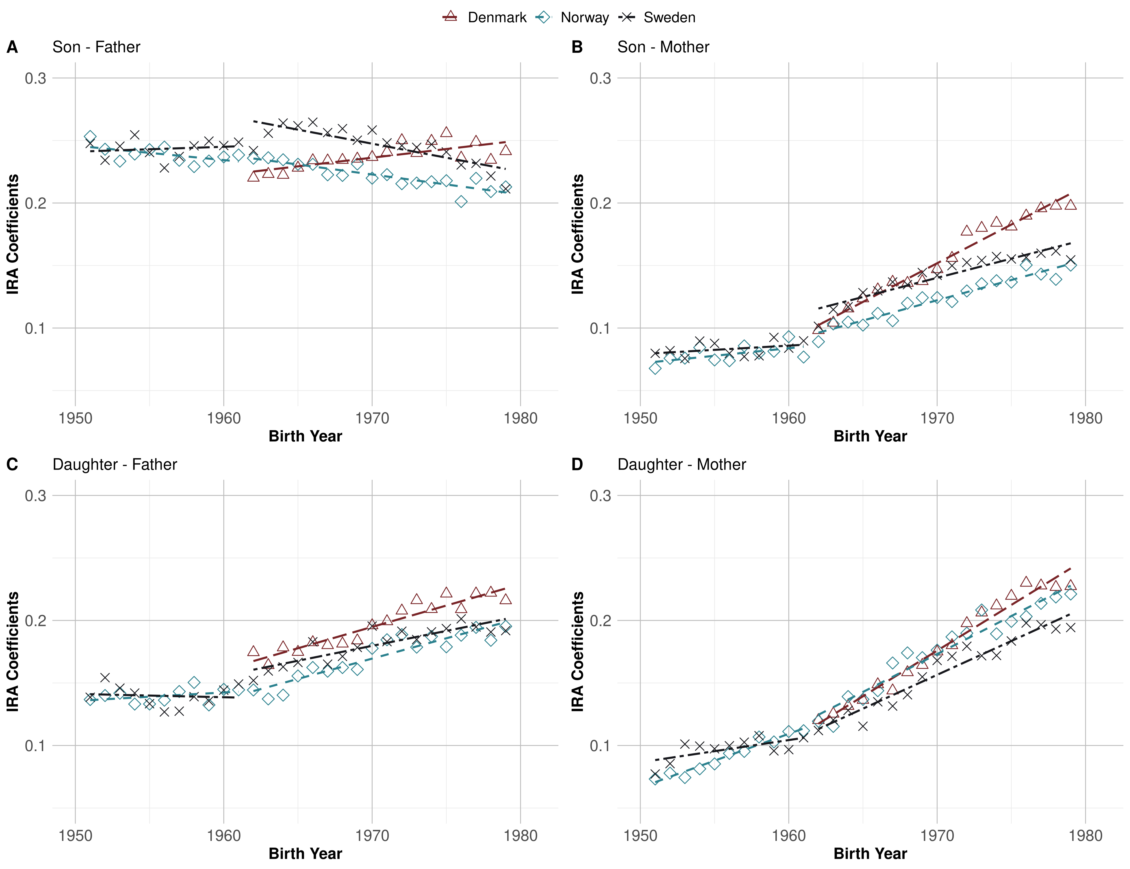
Figure 3: Trends in Intergenerational Mobility by Gender of the Parent and Child.

Notes: The four panels plot coefficients for the intergenerational rank association (eq. 1) in individual labor income for Denmark, Sweden and Norway, by child year of birth. Each panel provides estimates separately by gender of the parent and child. Each marker indicates the coefficient of a separate regression and each line indicates fitted trend lines separately for birth cohorts 1951 to 1962 and 1962 to 1979. “Birth Year” refers to birth year of the child in each parent-child pair.

Do these observed mobility patterns describe a phenomenon unique to Scandinavia? In order to understand this, we compute comparable mobility estimates for the US for birth cohorts from 1947 to 1983. Results from this exercise are presented in Table 1. US mobility trends are steepest for pairs involving women, and in particular daughters, while father-son rank associations appear to be relatively constant in the US, suggesting a comparable development to that observed in Scandinavia (similar results are shown in Song et al., 2020). However, the US trends in mother-son correlations are not statistically significant.

Another feature of Figure 3 and Table 1 is that earnings are more strongly related for parent-child pairs within gender (i.e., son-father and daughter-mother) than across gender (i.e., son-mother and daughter-father). In fact, while the association in earnings ranks is generally higher among sons and fathers than among any other combination of genders, the daughter-mother correlation reaches almost the same level towards the end of the considered period in Scandinavia. For the US, we only provide a pooled IRA coefficient due to the small sample. Nevertheless, the pattern that within-gender correlations are stronger than cross-gender correlations is also found in the US data.

Table 1: IRA Coefficients and Trends (United States).

	Parents	Father		Mother
	Child	Son	Daughter	Son	Daughter
Pooled IRA	0.317***	0.336***	0.195***	0.097***	0.137***
	(0.017)	(.022)	(0.031)	(0.025)	(0.029)
Trend $\times$ 100	0.603***	-0.240	0.980***	0.136	1.047***
	(0.149)	(0.205)	(0.277)	(0.253)	(0.292)
N	5,392	2,272	1,637	2,477	2,205

Notes: The table presents estimates of the IRA and linear trends in the IRA separately for different child-parent combinations. Due to the small sample sizes, trends have been estimated directly on the underlying micro data by regressing cohort-specific child ranks on cohort-specific parent ranks interacted with a linear time trend. The trend coefficients and corresponding standard errors have been multiplied by 100 in order to avoid too many digits after the separator. Estimates are based on the full sample of individuals in the PSID born between 1947 and 1983 using PSID sample weights. Standard errors are in parentheses. P-values indicated by * $<$ 0.1, ** $<$ 0.05, *** $<$ 0.01.

To the extent that father-son correlations, which are stable over time, credibly measure equality of opportunity, it is hard to argue that an actual decline in opportunity has taken place over time in either Scandinavia or the US. Thinking of the transmission of skills and values as something passive, this suggests that determinants of male income ranks, as well as the labor market valuation of skills that are passed on across generations, are unchanged over time. Instead, since all combinations of parent-child correlations that yield upward trends in IRAs (Panels B-D) involve women, a close-at-hand explanation lies in that women’s increasing integration into the labor force has changed the way that incomes are correlated across generations.

The difference in maternal trends between the US and Scandinavia would also be in line with such an explanation, as developments in female labor force participation started later in the United States and therefore likely impacted mothers only for later-born cohorts, while having a potentially larger impact through changing labor market equality for daughters.

4.4 The Importance of Female Labor Market Developments

We began this article by arguing that the changes in female labor supply seen in the past half-century could affect mobility trends in several different ways. This makes the sum of the different effects a priori unknown. In fact, evidence provided so far shows that parent-child rank correlations were relatively constant across birth cohorts 1951-1962, despite a great increase in maternal participation rates. Mechanically, whenever earnings are informative about heritable skills, we would expect mother-child earnings ranks to correlate more strongly at higher participation rates. The fact that this is not what we find speaks to a development where expansions on the extensive margin of employment happen in occupations where women’s skills are not well reflected in their earnings.

Next, we thus explore how the composition of the female labor force changed during the time of expanding female labor force participation in the 1950s and 60s. Figure 4 shows the relation between the change in the share of mothers in a given group of occupations, and the average years of education in that same group, for Norway and Sweden respectively, for birth cohorts 1951-1955 to 1961-1965 and 1961-1965 to 1975-1979.

From the early 50s to the early 60s, when labor force participation among mothers rose quickly, we see that women mainly entered relatively low-skilled occupations in both countries. In fact, in both Sweden and Norway, personal services occupations and secretaries together increase by almost 10 percentage points, which corresponds to about two-thirds of the increase in extensive margin employment among mothers. Under the assumption that pay in low-skilled occupations is not well differentiated across skills, the earnings of mothers remained uninformative of transmissible earnings potential, and mother-child earnings correlations did not increase.

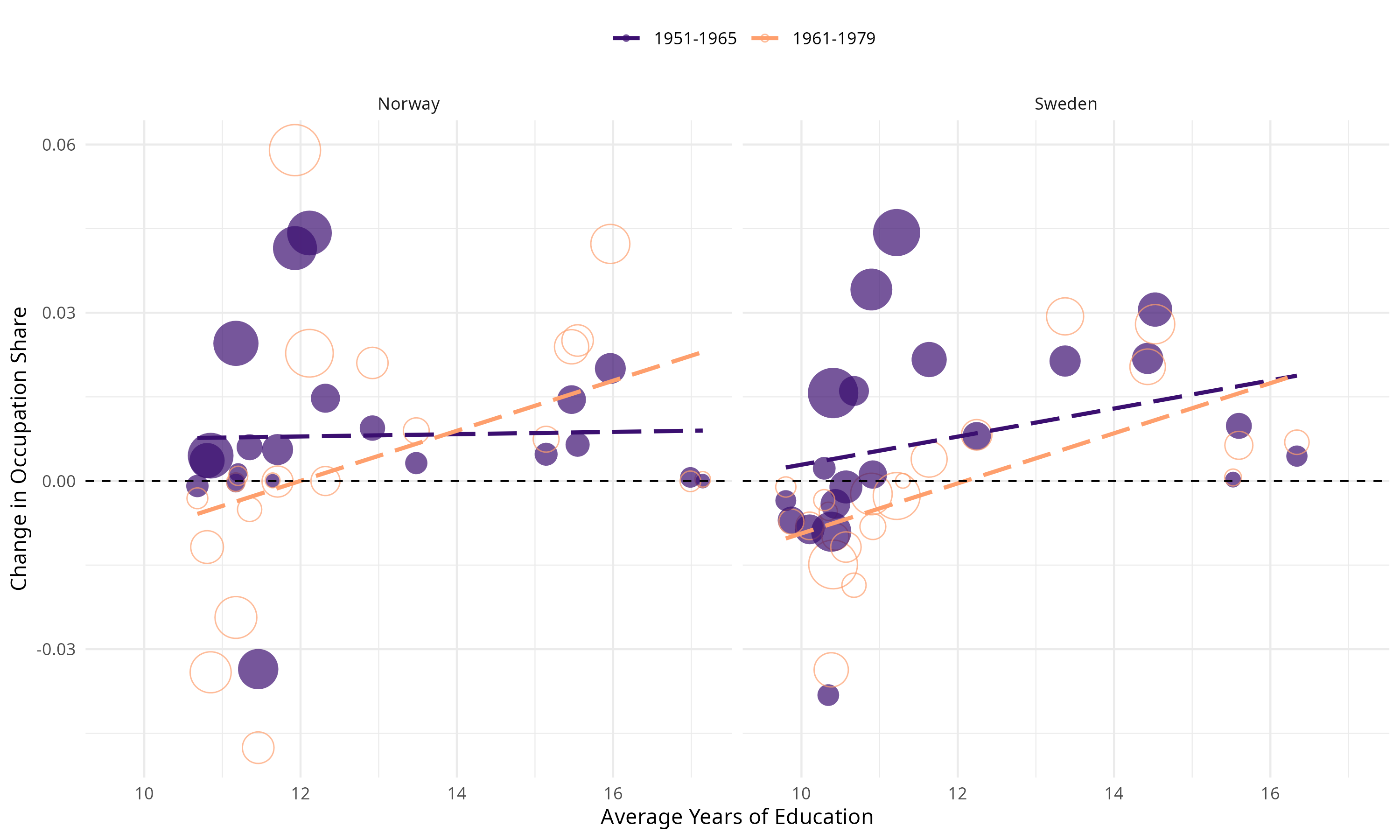
Figure 4: Changes in the Occupational Composition of Mothers.

Notes: The figure plots the average years of education within an occupational group (a proxy for the skill level of the occupation) against the change in the share of mothers with a job in that occupational group, from one group of birth cohorts to another. Each dot represents an occupational group, and the size of the dot represents the group size. Purple (filled) circles denote the change from mothers of the 1951-1955 birth cohorts to mothers of the 1961-1965 birth cohorts; orange (hollow) circles denote 1961-1965 to 1975-1979. Average years of education calculated in 1975-1979. Dashed lines represent the OLS fitted line between change in occupational share and average years of education, weighted by occupational size; purple for 1951-1965 and orange for 1961-1979. The left panel shows Norway and the right panel shows Sweden. Occupations are grouped as described in Appendix Table A2.

Conversely, our estimated gender-specific IRA trends for the period from 1962 to 1979 show that mother-son and parent-daughter earnings ranks converged rapidly in this period, while female labor force participation increased at a slower pace than before. From Appendix Figure B6 (which shows IRA-trends exclusively for individuals active in the labor market), it is also evident that extensive margin entry can not explain the increasing rank correlations in this time period, since correlations limited to only participants still display a trend toward lower mobility. Meanwhile, our descriptive statistics in Figure 1 (section 2) showed rapidly declining occupational segregation and increasing rates of full-time employment.

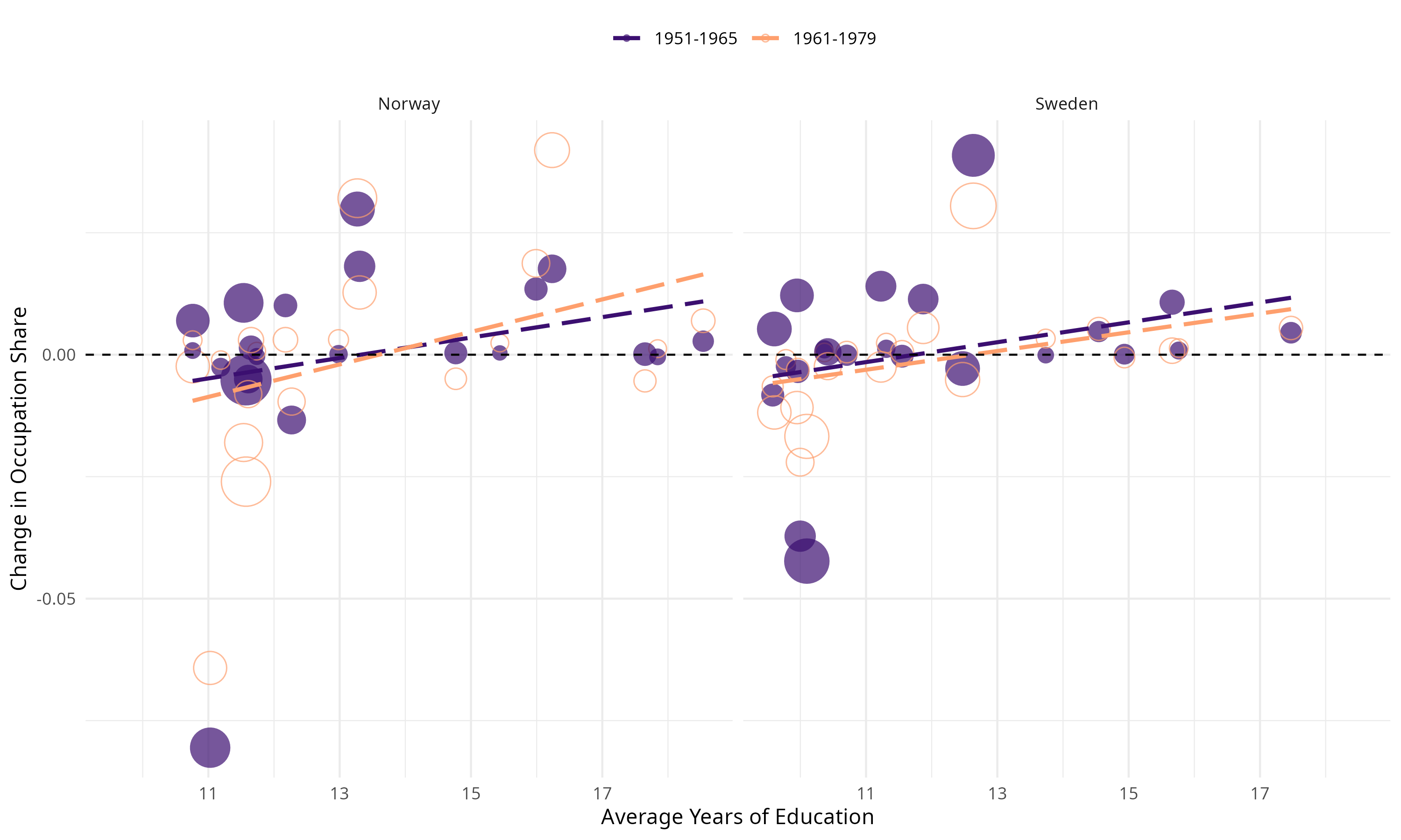
Figure B9: Changes in the Occupational Composition of Fathers.

Figure 4 shows that mothers with children born in this time period increasingly entered high-skilled occupations, while low-skilled occupations were declining. As extensive margin labor force participation did not change much during this time period, this implied a higher degree of sorting of workers into occupations, based on skills. Similar results for fathers indicate that there is almost no change in the way fathers sort into high-skilled occupations in both Norway and Sweden (shown in Appendix Figure B9). The average income rank of women in a particular occupation would thus become more reflective of their skill level, primarily through declining mean ranks of low-skilled occupations.

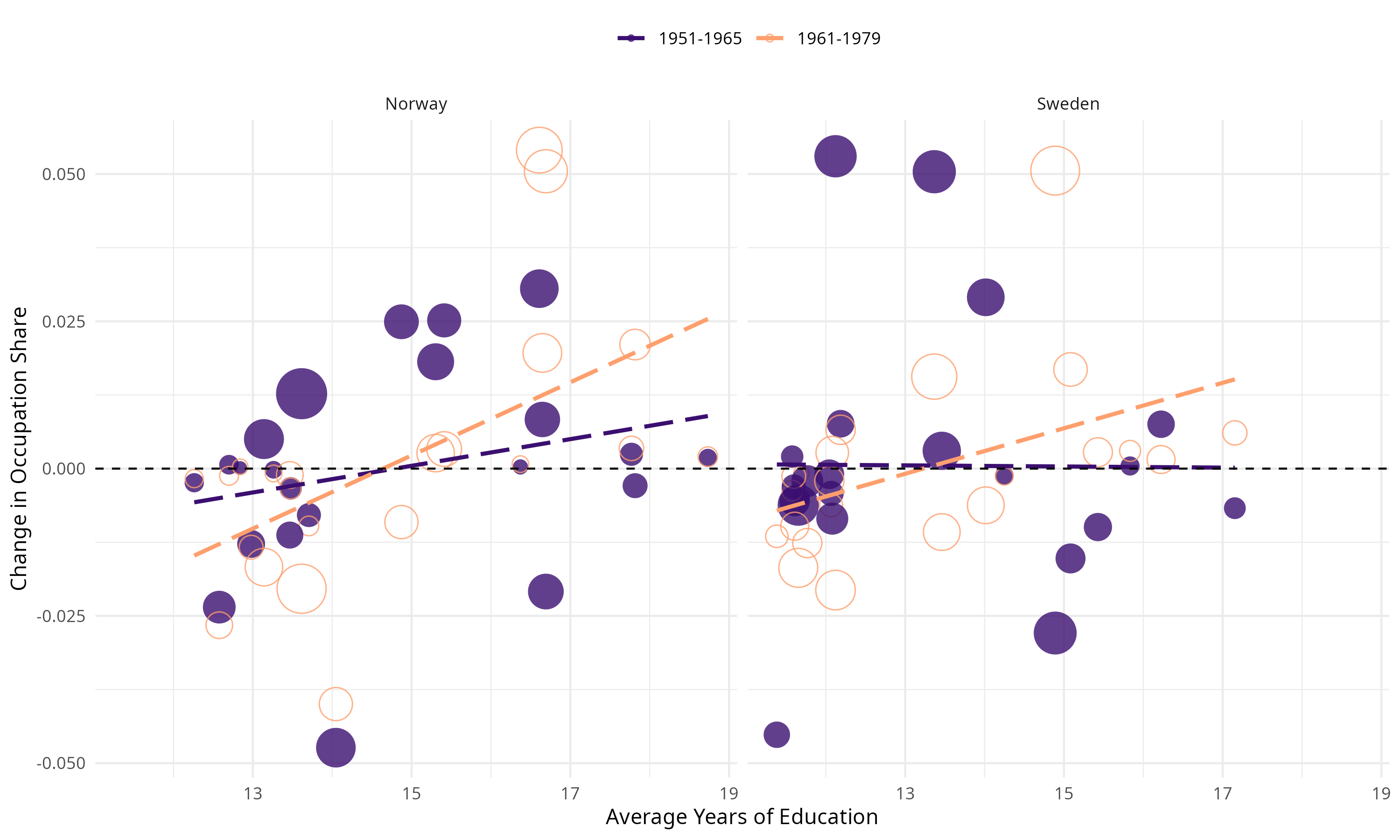
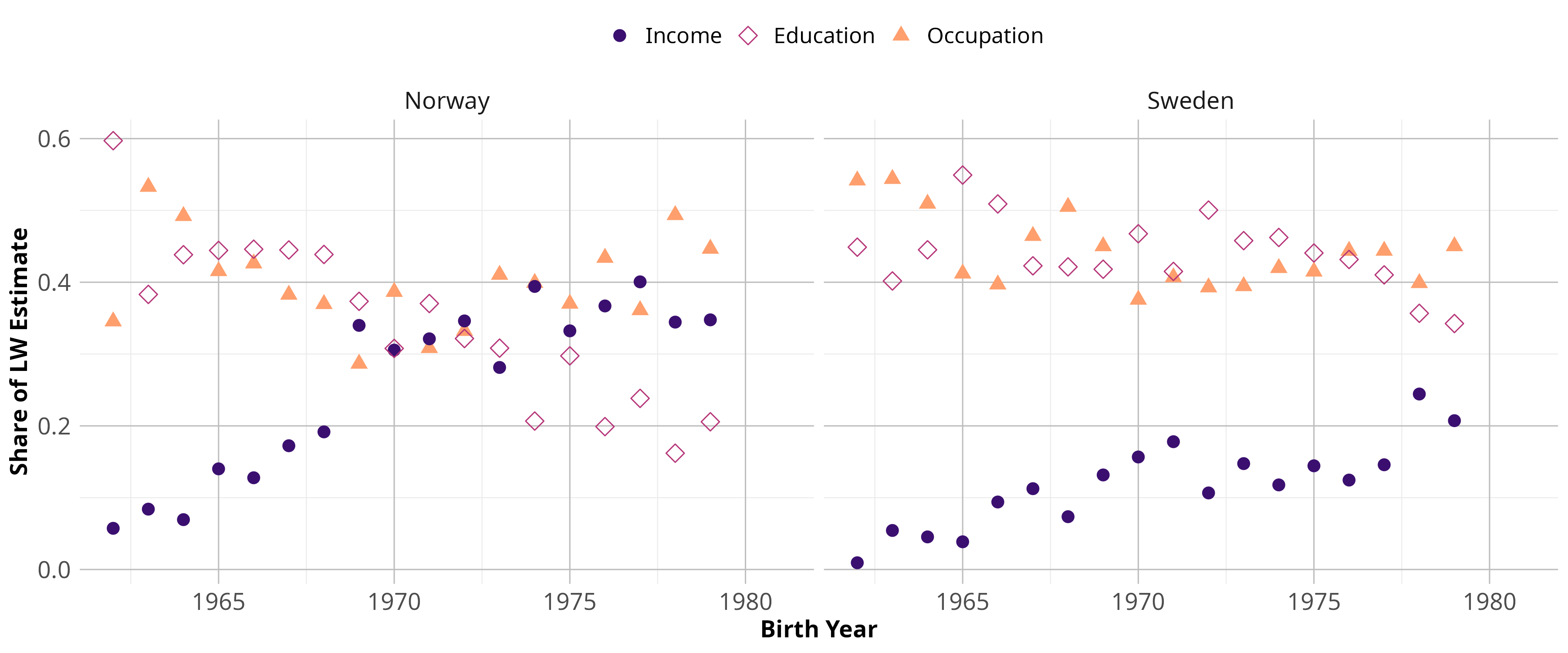
Figure B10: Changes in the Occupational Composition of Daughters.

In Appendix Figure B10, we show that the same patterns can be found among the daughters in our data set. Women born in the early 60s are evidently more likely to work than women born in the early 50s, but they work primarily in low-skilled occupations. Conversely, women born in the late 70s are less likely than those born in the early 60s to work in low-skilled occupations, while the share in high-skilled occupations is higher. Taken together, these findings indicate an increased level of sorting along skill levels in the economy. Thus, we may describe these later years as a period where female workers became better able over time to “earn their potential”.

5 Decomposition by Earnings Determinants

In the previous section, we documented that the intergenerational income rank association has increased rapidly in Scandinavia, but that this phenomenon is found almost exclusively for parent-child pairs involving mothers or daughters. Evidence regarding the occupational composition of mothers and daughters suggests that this results from changes in the extent to which female incomes reflect their inherent earnings potential (“skills”). However, our analysis might also be influenced by changes in the extent to which skills are transmitted across generations and by changes in assortative mating among parents. In this section, we build a simple model of intergenerational income persistence and use the gender-specific variation in mobility trends — along with correlations in parental earnings — to quantify the importance of different potential channels through a -decomposition exercise.

5.1 Model Setup and Calibration

In our framework, individual earnings at time $t$, $y^{k}_{it}$, are determined by two factors; inheritable skills, $x^{k}_{it}$, and a non-inheritable determinant $\varepsilon^{k}_{it}$. This generalizes to all fathers, mothers, sons, and daughters, i.e. all $k\in\{F,M,S,D\}$.

Interpreting these factors in the context of a highly simplified version of the frameworks formulated by Becker and Tomes (1979) and Solon (2004), we can think of $x^{k}_{it}$ as representing an aggregate measure of earnings determinants that can be transmitted across generations such as skills, values, and connections, while $\varepsilon^{k}_{it}$ represents the value of all other income determinants that are uncorrelated to skills that can be transmitted across generations (it may be instructive — yet slightly naïve — to think of this as luck). While $y^{k}_{it}$ is observable, the split between $x^{k}_{it}$ and $\varepsilon^{k}_{it}$ is fundamentally unobservable in the data. A similar approach to dividing income into inheritable and non-inheritable factors is also considered by Collado, Ortuño-Ortín and Stuhler (2022) in a more extensive framework.

We assume that inheritable skills in the parental generation follow a bivariate Gaussian distribution. In particular, we assume that

$$x_{it}^{F}\sim\mathcal{N}\left(0,1\right),\quad x_{it}^{M}=\left(\psi_{t}x_{it}^{F}+\left(1-\psi_{t}\right)u_{it}^{0}\right)/\Gamma_{t}^{0}$$ (2)

where $u_{it}^{0}\sim\mathcal{N}\left(0,1\right)$ and superscript ’0’ effectively denotes that the term refers to the parental generation. Standardizing the variance of maternal skills to one using $\Gamma^{0}_{t}$, $\psi_{t}$ reflects cohort-specific correlations in parental skills, thus measuring assortative mating in the model.

We assume that skills are transmitted passively from the parental generation to the child generation on the following form:

$$x_{it}^{k}=\begin{cases}\left(\kappa_{t}\left[\alpha_{t}x_{it}^{F}+\left(1-\alpha_{t}\right)x_{it}^{M}\right]+\left(1-\kappa_{t}\right)u^{1}_{it}\right)/\Gamma^{1}_{t},&\text{ for }k=S\\ \left(\kappa_{t}\left[\alpha_{t}x_{it}^{M}+\left(1-\alpha_{t}\right)x_{it}^{F}\right]+\left(1-\kappa_{t}\right)u^{1}_{it}\right)/\Gamma^{1}_{t},&\text{ for }k=D\end{cases}$$ (3)

Here, $\kappa_{t}$ is a measure of intergenerational correlation in inheritable skills — or the rate at which skills are transmitted — across generations within a given cohort of children, and $\alpha_{t}\in[0,1]$ is a coefficient that allows the transmission of inheritable skills within gender to be stronger than the transmission of inheritable skills across gender. Hence, whenever $\alpha_{t}>1/2$, then sons (daughters) inherit a relatively larger part of their inheritable skills from their fathers (mothers). The opposite holds when $\alpha_{t}<1/2$. Finally, $u_{it}^{1}$ is a stochastic element in the determination of skills which allows time-variation in the importance of intergenerational transmission of skills through variation in $\kappa_{t}$, and $\Gamma^{1}_{t}$ is once again a trivial scaling coefficient that ensures that the distribution of skills is standard normal — with ’1’ now pointing to the child generation.

Individual earnings are given by a monotone transformation of a linear index, which is composed of inheritable and non-inheritable determinants:

$$y_{it}^{k}=F_{t}^{k}\left(\tilde{\phi}_{t}^{k}x_{it}^{k}+\left(1-\tilde{\phi}_{t}^{k}\right)\varepsilon_{it}^{k}\right),\quad\text{for }k\in\{F,M,S,D\},$$ (4)

where $\tilde{\phi}_{t}^{k}=\nicefrac{{\phi_{t}^{k}}}{{\text{max}\left(\phi_{t}^{F},\phi_{t}^{M}\right)}}$ for $k\in\{M,F\}$ in the parental generation and $\tilde{\phi}_{t}^{k}=\nicefrac{{\phi_{t}^{k}}}{{\text{max}\left(\phi_{t}^{S},\phi_{t}^{D}\right)}}$ for $k\in\{S,D\}$ in the child generation, respectively. Parameters $\phi_{t}^{F}$ and $\phi_{t}^{M}$ measure the importance of inheritable skills relative to the non-inheritable component in the linear earnings index for fathers and mothers, respectively. Similarly, $\phi_{t}^{S}$ and $\phi_{t}^{D}$ measure the importance of inheritable skills relative to the non-inheritable component in the linear earnings index for sons and daughters. Making the simple assumption that the distribution of non-inheritable determinants can be summarized by a standard normal distribution, $\varepsilon_{it}^{k}\sim\mathcal{N}\left(0,1\right)$, the individual earnings index is also normal.

When measuring gender-specific intergenerational mobility in individual income ranks, the functional form of the monotone transformation function, $F_{t}^{k}(\cdot)$, is essentially unimportant; as long as it is monotone in the earnings index, any rank transformation of the earnings index will yield the same result as a rank transformation of earnings. However, in order to find both a joint measure of child income ranks across genders and a measure of joint parental earnings, the functional form can no longer be disregarded, since this would fail to take into account any gender differences in earnings distributions. Instead, we obtain the functional forms directly from the data. Exploiting the assumed monotone relationship between the earnings index and earnings, we match index ranks to the earnings distribution observed in the data. This allows us to compute pooled earnings ranks across genders in the child generation. We also compute a measure of joint parental earnings, $y_{it}^{P}$, that takes the true earnings distribution into account, as follows:

$$y_{it}^{P}=\hat{F}_{t}^{F}\left(\tilde{\phi}_{t}^{F}x_{it}^{F}+\left(1-\tilde{\phi}_{t}^{F}\right)\varepsilon_{it}^{F}\right)+\hat{F}_{t}^{M}\left(\tilde{\phi}_{t}^{M}x_{it}^{M}+\left(1-\tilde{\phi}_{t}^{M}\right)\varepsilon_{it}^{M}\right).$$ (5)

Here, $\hat{F}_{t}^{F}(\cdot)$ and $\hat{F}_{t}^{M}(\cdot)$ are cohort-specific estimates of the functions that map the earnings index to the earnings distribution observed in the data.

Table 2: Summary of Model Parameters

Parameter	Interpretation
$\psi_{t}$	Correlation in parental inheritable skills (assortative mating)
$\kappa_{t}$	Intergenerational correlation in inheritable skills
$\alpha_{t}$	The strength of within-gender skill transmission (relative to between-gender)
$\phi_{t}^{F}$	The relative importance of inheritable vs. non-inheritable skills for fathers
$\phi_{t}^{M}$	The relative importance of inheritable vs. non-inheritable skills for mothers
$\phi_{t}^{S}$	The relative importance of inheritable vs. non-inheritable skills for sons
$\phi_{t}^{D}$	The relative importance of inheritable vs. non-inheritable skills for daughters

For each country and cohort, we wish to calibrate a vector of seven decomposition parameters $[\begin{array}[]{ccccccc}\psi_{t}&\kappa_{t}&\alpha_{t}&\phi_{t}^{F}&\phi_{t}^{M}&\phi_{t}^{S}&\phi_{t}^{D}\end{array}]^{{}^{\prime}}$, summarized in Table 2, from the following five equations:

$$\text{Rank}_{it}^{\text{F}} =\alpha_{1t}+\beta_{1t}\text{Rank}_{it}^{\text{M}}+\varepsilon_{1it}$$ (6a)

$$\text{Rank}_{it}^{\text{F}} =\alpha_{2t}+\beta_{2t}\text{Rank}_{it}^{\text{S}}+\varepsilon_{2it}$$ (6b)

$$\text{Rank}_{it}^{\text{F}} =\alpha_{3t}+\beta_{3t}\text{Rank}_{it}^{\text{D}}+\varepsilon_{3it}$$ (6c)

$$\text{Rank}_{it}^{\text{M}} =\alpha_{4t}+\beta_{4t}\text{Rank}_{it}^{\text{S}}+\varepsilon_{4it}$$ (6d)

$$\text{Rank}_{it}^{\text{M}} =\alpha_{5t}+\beta_{5t}\text{Rank}_{it}^{\text{D}}+\varepsilon_{5it}$$ (6e)

In order to avoid underidentification, we make two adjustments. First, we set $\phi_{t}^{F}=\phi_{t}^{S}$. This means that the skill importance in earnings for mothers and daughters, $\phi_{t}^{M}$ and $\phi_{t}^{D}$, are interpreted relative to that of fathers and sons, respectively. In other words, we assume a generation-specific gender bias in the importance of skills for the determination of earnings. Secondly, we set $\phi_{t}^{F}=\phi_{t}^{S}=1$, thereby effectively pinning down the level around which $\kappa_{t}$ trends over time. The vector of decomposition parameters that are now left for us to calibrate across countries and cohorts is then given by $\left[\begin{array}[]{ccccccc}\psi_{t}&\kappa_{t}&\alpha_{t}&1&\phi_{t}^{M}&1&\phi_{t}^{D}\end{array}\right]^{{}^{\prime}}$.

5.2 Decomposition

By calibrating the model, we are eventually interested in understanding how country-specific changes in intergenerational mobility can be decomposed into changes in the rate at which inheritable skills manifest themselves in labor earnings among mothers and daughters relative to fathers and sons, and changes in assortative mating on skills among parents.

The calibration exercise can be summarized in four steps. First, we simulate data using the model that was outlined above and random values for the five model parameters. These data represent the initial period (1951 in Sweden and Norway, and 1962 in Denmark). Second, we estimate the slope coefficients in the five equations from the simulated data and compare these to those from our “real” data. Third, we utilize a form of gradient descent algorithm in order to improve the fit of the simulated data, by adjusting the model parameters. The model fit is evaluated by the difference between the slope coefficients in the “real” and the simulated data. Fourth, we re-simulate the data based on these adjusted model parameters. Steps two to four are repeated iteratively until a stopping criterion is met. This stopping criterion is a function of the quality of the model fit as well as the rate of convergence. When the final set of calibrated model parameters for a given cohort is found, we move on to the next cohort of children (say, 1952 in Sweden and Norway, and 1963 in Denmark) and utilize the final set of calibrated model parameters from the previous period as the starting point for the new period. The calibration procedure is explained in greater detail in Appendix section C, where we also document the quality of the calibration exercise for each set of country-cohort combinations of parameters.

Table 3: Estimated Values of the Model Parameters for Cohorts 1951, 1962, and 1979.

			1951				1962				1979
			SE	DK	NO		SE	DK	NO		SE	DK	NO
	$\psi_{t}$		0.131	-	0.147		0.289	0.189	0.171		0.249	0.186	0.174
	$\kappa_{t}$		0.301	-	0.300		0.257	0.267	0.274		0.261	0.290	0.286
	$\alpha_{t}$		0.580	-	0.603		0.632	0.582	0.626		0.561	0.560	0.564
	$\phi^{M}_{t}$		0.286	-	0.260		0.368	0.398	0.371		0.594	0.701	0.622
	$\phi^{D}_{t}$		0.511	-	0.501		0.591	0.721	0.619		0.935	1.011	0.951

Notes: The table presents calibrated decomposition parameters for Sweden (SE), Denmark (DK), and Norway (NO) in three selected cohorts. These cohorts represent the start of the Swedish and Norwegian data, the start of the Danish data, and the final cohort in the sample. The coefficients have been obtained by matching a simulated version of the model described in Section 5.1 to the gender-specific IRA coefficients observed in the data, as well as the relation between father and mother income.

Before turning to the importance of each parameter in explaining trends in intergenerational income mobility, we first investigate how the model parameter estimates change over time in the calibration exercise. Parameters for the cohorts 1951, 1962, and 1979 are displayed in Table 3. Several noteworthy features stand out. First, the decomposition parameters generally evolve similarly across countries, which adds credibility to the exercise. In particular, the parameters associated with skill-importance in earnings for mothers and daughters, $\phi_{t}^{M}$ and $\phi_{t}^{D}$, have increased at a somewhat similar pace across all three countries. This suggests that female earnings may have become more reflective of inheritable skills in both the parent and child generations.

Second, the parameter associated with assortative mating, $\psi_{t}$, is rather stable over time in all three countries, in spite of strongly increasing associations in maternal and paternal earnings over time (which is displayed in Appendix Figure C1). This may result from the increased reflection of maternal inheritable skills in earnings, which mechanically increases the observational correlation in father and mother earnings for a given correlation in skills (assortative mating).

Third, within-gender intergenerational correlations in inheritable skills do in fact seem to be stronger than cross-gender correlations in skills — $\alpha_{t}$ is approximately 0.6 across all countries but slowly declining from the early 1960s and onward. Finally, the parameter associated with non-gendered skill transmission, $\kappa_{t}$, is stable over time.

While the trends in decomposition parameters are generally similar across countries, the direction and extent to which they may affect the intergenerational rank association in earnings between parents and children is a priori unknown. In order to decompose changes in rank associations into effects associated with changes in the modeling parameters, we compute “counterfactual” earnings associations through the following process. First, we re-simulate the model using our calibrated time-specific parameters while holding one parameter fixed at the calibrated value from some baseline period (say, cohort 1962). Second, we re-compute the intergenerational rank associations with this “counterfactual” set of model parameters. Differences in estimated intergenerational rank associations are attributed to the parameter that was held fixed.

More technically, we first define $\tilde{\beta}_{t}$ as the rank association between joint parental earnings and child earnings obtained from the simulated data (using the calibrated set of parameters). Hence we may define $\tilde{\beta}_{t}\equiv\beta\left(\psi_{t},\kappa_{t},\alpha_{t},\phi_{t}^{M},\phi_{t}^{D}\right)$. Then, we define $\tilde{\beta}_{t,\underline{t}}^{b}$ in a similar fashion, but we fix one parameter $b_{t}\in\left(\psi_{t},\kappa_{t},\alpha_{t},\phi_{t}^{M},\phi_{t}^{D}\right)$ to the calibrated value in period $\underline{t}$. For instance, $\tilde{\beta}^{\psi_{\underline{t}}}_{t}\equiv\beta\left(\psi_{\underline{t}},\kappa_{t},\alpha_{t},\phi_{t}^{M},\phi_{t}^{D}\right)$. Finally, the part of the trend in $\tilde{\beta}_{t}$ that can be attributed to parameter $b$ is simply the difference in trend between $\tilde{\beta}_{t}$ and $\tilde{\beta}^{b}{t,\underline{t}}$, while the part of the actual trend in $\beta_{t}$ that can jointly be attributed other factors than decomposition parameters and changes in the aggregate gender-specific income distributions is the difference in trend between $\beta_{t}$ and $\tilde{\beta}_{t}$. The results from this exercise are shown in Table 4.

Table 4: Results from the Decomposition Exercise for Cohorts 1951-1962 and 1962-1979.

			1952-1961				1962-1979
			SE	DK	NO		SE	DK	NO
	Trend in $\beta_{t}$		0.013	-	0.140		0.277	0.530	0.379
	Trend in $\tilde{\beta}_{t}$		0.068	-	0.138		0.240	0.527	0.327
	Due to $\psi_{t}$		0.189	-	0.000		-0.056	-0.001	0.001
	Due to $\kappa_{t}$		-0.343	-	-0.164		-0.041	0.242	-0.035
	Due to $\alpha_{t}$		0.009	-	0.007		0.002	0.000	0.001
	Due to $\phi^{M}_{t}$		0.054	-	0.117		0.138	0.220	0.161
	Due to $\phi^{D}_{t}$		0.020	-	0.130		0.158	0.069	0.119

Notes: The table presents trends in observational IRA coefficients, $\beta_{t}$, in the three countries as well as trends in IRA coefficients obtained from the calibrated models in the three countries, $\tilde{\beta}_{t}$. The contribution from each parameter is computed as the difference in $\tilde{\beta}_{t}$ that is obtained from holding one calibrated parameter fixed at a time. The sum of contributions from each parameter need not sum to the trend in $\tilde{\beta}_{t}$ as part of the trend will be driven by changes in the scale of gender-specific income distributions which is not modeled.

As the rank associations in earnings did not exhibit any clear upward trend for cohorts born between 1952 and 1961 in Sweden and Norway, there is not much to be explained by the decomposition parameters. However, there are certain noteworthy patterns in this period. In particular, the parameter associated with non-gendered skills transmission, $\kappa_{t}$, contributes negatively to the IRA over time, while the opposite is the case for the parameters associated with the extent to which female earnings are reflective of parental skills, $\phi_{t}^{M}$ and $\phi_{t}^{D}$. This could possibly suggest that passive skills transmission may in fact have declined over time, thereby improving income mobility, but that this effect was mitigated by the increasing extent to which women’s individual income reflects their earnings potential.

For birth cohorts 1962 to 1979, the simulated data capture the fact that IRAs are increasing uniformly across Scandinavia remarkably well. Both parental assortative mating ($\psi_{t}$) and gender-specific skill transmission ($\alpha_{t}$) generally contribute little to mobility trends in this period. Our results suggest a bigger role for gender-neutral skill transmission ($\kappa_{t}$) — at least in Denmark, where this component explains almost half of the observed trend in mobility. In both Sweden and Norway, however, the contribution of $\kappa_{t}$ is negative and the importance is negligible. Changes in the extent to which female earnings (and particularly maternal earnings) are driven by inheritable skills ($\phi_{t}^{M}$ and $\phi_{t}^{D}$) are found to be important drivers of downward trends in mobility across Denmark, Norway, and Sweden. These effects jointly contribute to a yearly increase in the earnings IRA of between 0.28 and 0.30 rank points in all three countries, amounting to a total increase in the IRA of between 5 and 6 rank points over the period. Taking this result at face value would thus suggest that increased labor market valuation of female skills alone can explain most of, or even the entire, observed decline in intergenerational income mobility in Scandinavia.

6 Intergenerational Correlations in Latent Economic Status

The central hypothesis in this paper is that changes in female labor market conditions introduce a progressively lesser degree of measurement error in the estimated trends in parent-child correlations in economic status. The purpose of this section is to estimate trends in intergenerational mobility that are less affected by this bias, and thereby potentially validate the model-based findings of Section 5.

We thus follow recent work by Vosters and Nybom (2017), Vosters (2018) and Adermon, Lindahl and Palme (2021) and apply the method laid out in Lubotsky and Wittenberg (2006) (from now on “LW”). The intuition behind this method is that observable variables constitute imperfect measures of a person’s underlying, or “latent”, socioeconomic status, but that a less attenuated measure of economic status can be constructed from a weighted average of several proxy variables. In essence, it uses a set of proxy variables that together represent a single latent variable — here, economic status — and sums these with “optimal weights”. These weights are calculated as the covariance between a given outcome variable (in our case, child income) and the proxy variable, and have been shown to result in an estimator that minimizes attenuation bias among its class of estimators (Lubotsky and Wittenberg (2006), p.552). The procedure requires the theoretical assumption that each proxy measure affects the left-hand side variable — child economic status — only through latent economic status, but it does not assume independence between the proxy variables.

We use income, years of education, and occupation as proxy variables for the economic status of mothers (and fathers, as a validation exercise). Income is included for two reasons. First, to gauge the informational value of individual labor income for latent economic status, and how this changes over time. Second, it serves as a denominator for the other proxies: education and occupation are expressed on a fixed scale. Aside from being essential to the method, including income allows for a direct comparison between the LW estimates and our results using income ranks. As in previous applications, we use the logarithm of child and parent labor income to calculate the LW estimates. In order to use the same full-population sample as in our main analysis, we assign individuals with zero labor income a token low level of log earnings. Sensitivity checks show that the exact level of earnings assigned does not alter the conclusions from this analysis.

For occupations, we follow Vosters and Nybom (2017) and include a dummy variable for each of ten occupational groups. These are roughly equivalent to 1-digit ISCO codes: professional, managerial, clerical, commerce, agriculture, mining, transportation, manufacturing, military and services. An additional dummy variable is included for missing occupational information. See Appendix A for a full description of how we assign individuals to occupations and divide occupations into groups.

The proxy variables are denoted $x_{j},\quad j\in{1,..,k}$. The LW estimator for the parents with children born in year $t$ is constructed as follows:

$$\beta^{LW}_{t}=\sum_{j=1}^{k}\rho_{j}b_{j},$$ (7)

where $\rho_{j}=\frac{cov({Income}_{it}^{\text{C}},x_{jit})}{cov({Income}_{it}^{\text{C}},{Income}_{it}^{\text{P}})}$ is the weight on proxy variable $j$. This is essentially a Wald estimator: the covariance between child income and proxy variable $j$, scaled by the covariance between child and parent income. As such, it can be calculated with a 2SLS estimator. Since parent income serves as the denominator, the weight on the parent income, $\rho_{1}$, is equal to one. The $\mathbf{b_{j}}$’s are OLS coefficients from a multiple regression of child income on the set of parent proxy variables. Summing $\rho_{j}b_{j}$ over all proxy variables gives the estimate $\beta^{LW}_{t}$.

In order to compare the estimates to IRAs, we want to correlate parent ranks in economic status to child income ranks. We thus transform the parental LW estimates into percentile ranks, using the explicit index construction mentioned in Lubotsky and Wittenberg (2006) (p.554):

$$x_{it}^{\rho,\text{P}}=\frac{1}{\beta^{LW}_{t}}\sum_{j=1}^{k}x_{jit}b_{jt},$$ (8)

Finally, we regress the child income ranks on these parental index ranks, for mothers and fathers separately, and for each birth cohort. Note that our main goal is not to provide point estimates for mother-child correlations in economic status, but rather to assess the development over time. We estimate:

$$\text{IncomeRank}_{it}^{\text{C}}=\alpha_{t}+\beta_{t}x_{it}^{\rho,\text{P}}+\varepsilon_{it}.$$ (9)

The method described so far addresses the problem of unrepresentative maternal earnings: if trends in intergenerational rank correlations in latent economic status between mothers and sons resemble income rank correlations between fathers and sons, it stands to reason that the upward trend in mother-son earnings correlations can be attributed to increased economic opportunities of women, and subsequently less attenuation bias. In order to understand whether daughter-father correlations are subject to the same issue (and bias in estimation), we repeat the above procedure for daughters and approximate their economic status with income, education, and occupations. Since the LW method addresses measurement error in the right-hand-side (independent) variable, this requires “flipping” the intergenerational model (eq. 1), and estimating rank associations between fathers and their daughters:

$$\text{Rank}_{it}^{\text{P}}=\alpha_{t}+\beta_{t}\text{Rank}_{it}^{\text{C}}+\varepsilon_{it}.$$ (10)

This has only minor impacts on the year-specific IRA estimates and does not alter the trend. Apart from this first step, we proceed in an identical manner to the son-mother estimation.

6.1 Results

Figure 5 plots the trend in IRA and LW estimates for birth cohorts 1962 to 1979, separately by country. We focus here on the birth years 1962-79 because we observe the largest increase in rank correlations for this part of the sample. In Appendix Table B7, we also report the difference between the trend estimates and test whether trends in intergenerational rank associations are statistically distinguishable between the IRA and LW approaches.

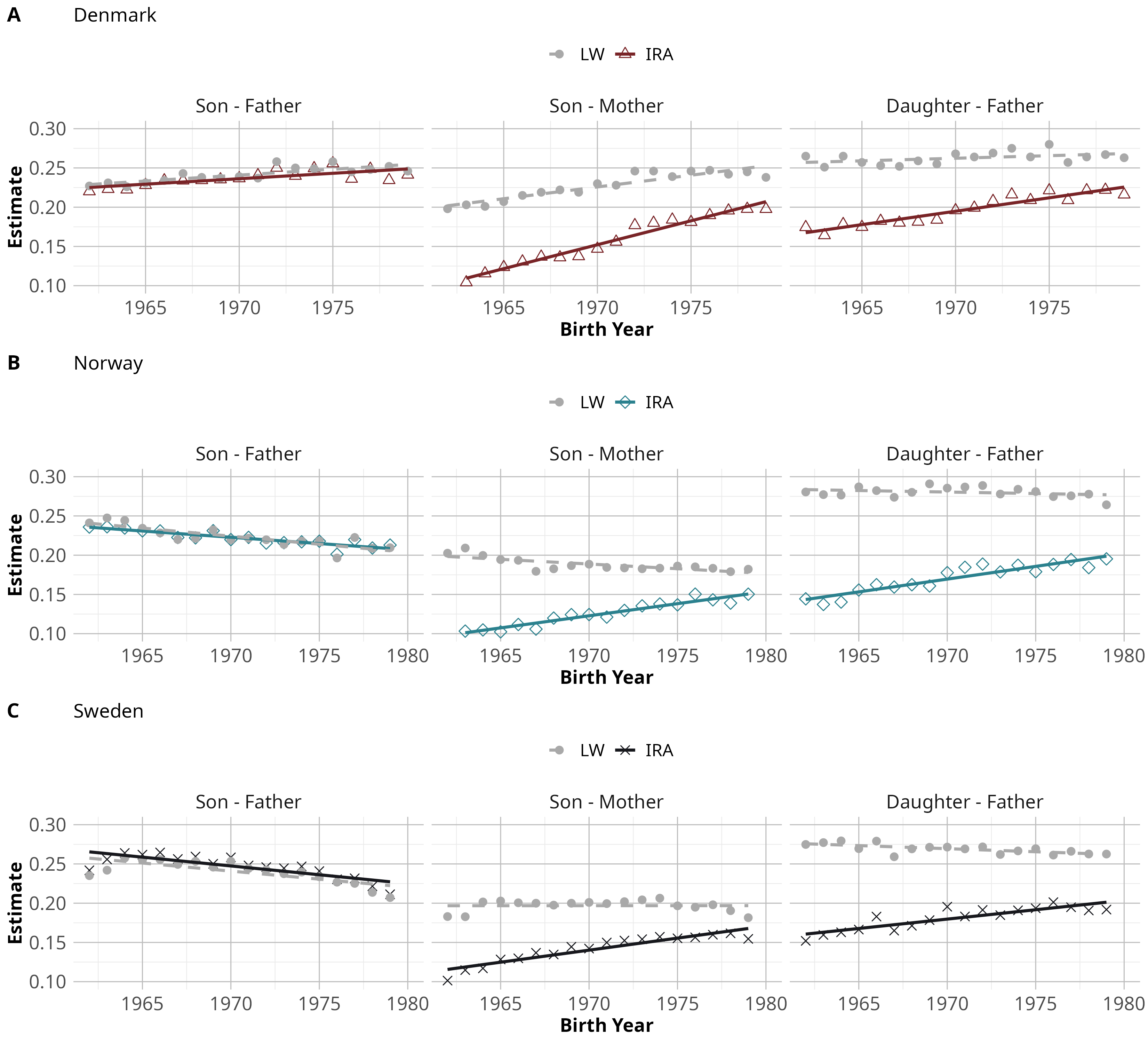
Figure 5: Trends in Intergenerational Mobility in Latent Economic Status.

Notes: The three panels plot comparisons of intergenerational rank associations and rank associations in latent economic status (calculated using the proxy variable method from Lubotsky and Wittenberg (2006)) for Denmark, Sweden and Norway. Each panel shows, in turn, son-father, son-mother and daughter-father correlations. Each marker indicates the coefficient of a separate regression (eq. 7 for LW; eq. 1 for IRA) and each line indicates fitted trend lines for the period 1962 to 1979. “Birth Year” refers to the birth year of the child in each parent-child pair.

The first column of Figure 5 shows that the son-father trends obtained from the LW method are almost identical to the son-father IRA trends, which validates that the proxy variable method captures the rank-rank association in economic status. When income is fully informative of economic status, the LW weighting procedure yields the same result as income rank correlations. For Norway and Sweden, IRA and LW trends are negative, indicating a development towards increased mobility, while Denmark’s decline in mobility is supported by both the IRA and LW methods.

The middle column shows son-mother estimates. Compared to the IRA trend, our LW trends are noticeably weaker, and in the case of Norway even negative. This suggests a development similar to that of father-son estimates. The difference between the trends in the IRA and LW coefficients is statistically meaningful and different from zero, and also similar in magnitude across all three countries. The LW method thus mitigates attenuation bias to approximately the same extent across countries. Evidently, when using mothers’ years of education and occupations - rather than just labor earnings - to proxy for their latent economic status, income persistence between male children and their mothers, as well as their fathers, has remained relatively constant over time.

In the Appendix (Figure B11), we show that both education and occupations contribute independently of one another to the rank correlations between mother economic status and son income rank. Moreover, the degree to which maternal education is correlated with child earnings declines gradually over time, while the correlation between son and mother incomes increases. Maternal occupations continue to contribute more than either education or income to the LW estimates throughout our sample period, which suggests that still for mothers of the late 70s cohorts, occupational choices carry greater informational value than their annual income.

In the last column of Figure 5, we present comparisons between trends in LW and IRA coefficients for daughters and fathers. Again, the LW trends are significantly less steep than the IRA trends. The differences between them are again almost identical across countries. For Denmark, the adjusted trend still indicates that over time, mobility in economic status decreases, albeit at a lower rate. In Norway, the relationship is stable, while daughters in Sweden experience a small increase in mobility over time. In summary, these results provide three important takeaways. First, son-father LW trends are similar to IRA trends, indicating that the IRA captures the development of intergenerational mobility in latent economic status. Second, trends in the son-mother and daughter-father IRA appear to overestimate declines in mobility, and, third, differences in trends between the IRA and LW methods are comparable across countries.

In addition to the comparison of trends, the levels of the son-father, son-mother, and daughter-father LW coefficients are more similar to the IRA coefficients of son-father pairs, as would be expected when accounting for attenuation in the coefficients (and this result is also supported by findings in Vosters and Nybom (2017)). Estimating rank associations in latent economic status by birth cohort shows that over time, father-daughter correlations have remained roughly constant at a level just below 0.3. The transmission of economic potential between parents and their female children, as well as their male children, has thus seen little change across birth cohorts from 1962 to 1979. This might reflect the Scandinavian setting, with relatively equal schooling opportunities among boys and girls already for individuals born in the 1950s. The fact that father-daughter correlations are as high as the father-son ones suggests that whatever skills relevant to economic success are transmitted between parents and their children, these are gender-neutral.

By estimating correlations in “latent economic status” rather than observed income, our goal is a measure that better approximates the transmission of income-generating skills between parents and their children. One could argue, however, that the occupational and educational choices of women historically suffer from the same low correlation with underlying skills as does income. To corroborate the LW results, we also estimate the intergenerational rank association in labor income between sons and their maternal uncles. Given a constant level of brother-sister correlation in earnings potential (Björklund, Jäntti and Lindquist, 2009), this estimated trend captures changes in the importance of parental earnings potential for child outcomes. Using observed skills of maternal uncles to proxy for unobserved female values is a strategy previously used by e.g. Grönqvist, Öckert and Vlachos (2017). Because the data needed for generating parental sibling links is partly unavailable, the sample size used to estimate these correlations is smaller, particularly for the earliest birth cohorts, and Denmark is left out of the analysis.

Figure 6 presents the results. Panel A shows a constant level of rank associations over time between sons and their maternal uncles. Panel B shows the original mother-son associations for comparison, and in Panels C-D, the same results are shown for daughters and maternal uncles. Daughter-uncle trends are substantially flatter than daughter-mother trends, indicating that a certain part of the mother-daughter trends is driven by the mothers. However, the remaining IRA trend shows that increased labor force attachment by daughters over time also contributes to the observed mobility trend.

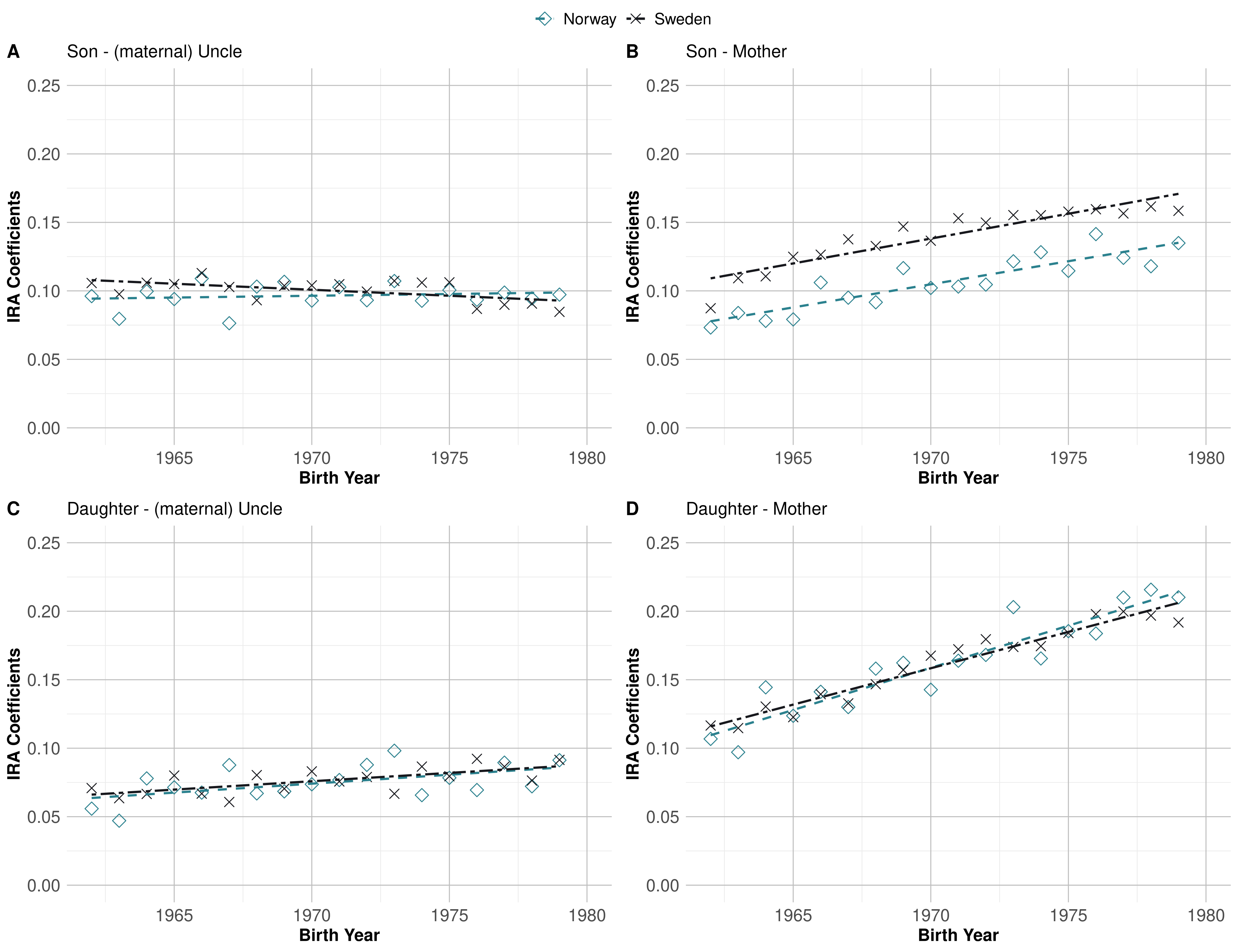
Figure 6: IRA Estimates Between Children and Their Maternal Uncles.

Notes: The four panels depict IRA coefficients (eq. 1) for the correlation between children and their mother’s brothers, i.e. maternal uncles; Sons in Panel A and daughters in Panel C. Panels B and D show the estimated IRA between sons and daughters and their mothers for the sample where information on maternal uncles is available. “Birth Year” refers to the birth year of the child in each parent-child or uncle-child pair. Results for Sweden are depicted in dark X’s, Norway in hollow diamonds (Denmark is left out of this analysis due to data availability).

7 Conclusion

In this paper, we document trends in intergenerational income mobility in Denmark, Norway, and Sweden, for children born between 1951 and 1979. Harmonizing data and definitions, we show that the intergenerational rank association between parents and children in individual labor earnings has increased significantly in all three countries. These trends are robust to using different types of income measures, as well as to restricting the analysis to labor market active individuals. Splitting trends by gender of parents and children, son-father correlations exhibit the weakest trend in all three countries, whereas all correlations involving mothers and daughters increase over time. The strongest trend is found between mothers and daughters. We also show that a similar, but delayed, pattern of changes in mobility can be found for US parent-child pairs from the Panel Study of Income Dynamics.

Our results suggest that increasing female labor supply at the extensive and intensive margin results in higher child-parent rank associations. We show that this is the result of better manifestation of skills in income for women, such that the intergenerational correlation in “potential income”, or latent economic status is revealed. In other words, the fact that maternal economic status was poorly reflected in maternal income among early cohorts of our sample caused rank associations between child income and joint parental income to be an attenuated measure of mobility in economic status, or “opportunity”. Over time, as female labor force participation has increased and women are better able to choose occupations that match their inherent skills, this attenuation has declined.

These results highlight the importance of accounting for changes in female economic status when estimating trends in intergenerational mobility. The interpretation that higher income rank associations between children and parents reflect a lower degree of social mobility or equality of opportunity is not always easily applicable when labor market conditions change substantially. Our findings suggest that over time, female income becomes increasingly determined by their earnings potential, meaning that the traits and norms that women inherit from their parents are also better reflected in their income. While such a development must be seen as a necessary side-effect of increased gender equality in the labor market, it is not clear whether it should be seen as a reduction or advancement in equality of opportunity.

Appendix

Appendix A Data Registers and Variable Definitions

Denmark

The Danish income registries start in 1980 and contain detailed information on the individual income composition of Danish adults. The registries are based on information from the Danish tax authorities, supplemented with information from other Danish authorities, including unemployment insurance funds and local authorities.

The measure of labor income that is being used in this paper consists of wage payments (incl. non-wage benefits, non-taxable wage payments, stock options, and more) and any net surplus from own, private company. Gross income is equal to labor income, transfers, property income, and any other non-classifiable income that the individual may have received throughout the year. Net-of-tax income is finally equivalent to gross income net of all taxes that have been paid to either the government, municipalities, or other public authorities. Individuals with no parents in the sample (generally people who moved to Denmark, whose parents have moved abroad, or whose parents are deceased) are naturally dropped from the sample. In order to ensure comparability between income definitions across countries, negative observations of income have been set to income.

When constructing household income measures, individuals are being linked to their spouses. In the Danish sample, a spouse is generally defined by marriage, registered partnership or registered as a cohabiting couple. Matching individuals to spouses as well as parents is done using the population registries of Denmark.

Occupation data are obtained from the Danish employment classification module, AKM. Occupations are characterized by the Danish ISCO classification system (DISCO) and only observable from 1992 and onward. In order to impute data from 1980 to 1991, we use a random forest-algorithm in order to map a range of occupation-related variables to occupation codes in 1992. We then use this mapping in order to characterize individual occupations from 1980 and up until 1990 where the occupation codes are missing. Starting from 1991, there is a range of data-breaks in the sense that certain types of occupations are re-classified, split up or gathered into one group. In order to make occupations as comparable as possible over time, we re-classify occupations across years so that classifications are approximately constant over time. For certain individuals, the occupational status is either unknown or missing. These are instead assigned to the occupational status that was observed most recently within a window of +- 3 years. Due to these imputation and re-classification procedures, any results in this paper that rely on occupation codes from Denmark should be interpreted with some caution.

Information on individuals working part time is obtained from a matched employer-employee data module, IDAP. For a series of individuals (people who are not self-employed and do not have multiple occupations), full time work is assessed in a relatively straightforward way. In cases of doubt (individuals are e.g. self-employed or have multiple part-time occupations), we assign full employment status to a individual whose labor income amounts to at least the mean labor income of full-time employed individuals (specifically, full-time employed individuals whose earnings fall within the range of the 15th and 25th earnings percentile as observed within the same age-category). Up until 2007, full-time work is classified as at least 27 weekly hours. From 2008 and onward, the equivalent number is 32. This data break does not show up in the parental generation in our sample (as these are observed up until 1998). In the child generation, gender-specific full time rates are re-scaled in the following way in order to account for the data-break when computing aggregate cohort- and gender-specific statistics:

$$\widetilde{\mathrm{ftr}}_{t}^{g}=\begin{cases}\mathrm{ftr}_{t}^{g},&\text{ if }t<1971\\ \widehat{\mathrm{ftr}}_{t}^{g},&\text{ if }t=1971\\ 1-\left(1-\mathrm{ftr}_{t}^{g}\right)\frac{\left(1-\widehat{\mathrm{ftr}}_{1971}^{g}\right)}{\left(1-\mathrm{ftr}_{1971}^{g}\right)},&\text{ if }t>1971\end{cases}$$

where $\widetilde{\mathrm{ftr}}_{t}^{g}$ are the full time rates that we report in Figure 1, ${\mathrm{ftr}}_{t}^{g}$ are full time rates as observed in the data (hence, without accounting for the data break) and $\widehat{\mathrm{ftr}}_{t}^{g}$ is the fitted gender-specific full time rate in 1971 that is obtained from a linear regression of full time rates, ${\mathrm{ftr}}_{t}^{g}$, on $t$, using full time rates from 1966 up until 1970.

An individual’s level of education reflects the highest obtained level of education. In some years, the duration of the education is not available in the data. In these cases, the duration of the education is either imputed from the duration of that same education in an earlier year, or it is imputed from educations that are characterized as being similar.

Norway

Our Norwegian data set combines information from the central population registry with information about income and earnings from the tax registry. Income data in Norway is available from 1967 to 2018. Labor income includes payments related to employment, including overtime pay, taxable sickness benefits, parental leave pay, short-term disability pay, and rehabilitation benefits. This is top-coded for a few years in the 1970s at the maximum amount for contributions to the national social security scheme (folketrygden). Gross income is the sum of labor income and taxable and non-taxable transfers and income from capital. Disposable income is defined as gross income minus taxes and is also sometimes referred to as net-of-tax income. The definitions change somewhat over time due to reforms of the benefit, insurance, and tax system. For the net-of-tax and gross income variable, the data series ends in 2014, which is why these income measures are constructed from more detailed income data only available from 1993. Spouses (married couples as well as couples in civil unions) are linked through their personal identifiers

The occupation data used for implementing the method proposed by Lubotsky and Wittenberg (2006) is pooled from matched employer-employee data (Registerbasert sysselsettingsstatistikk) available annually starting with the year 2000. In addition occupation data from the censuses 1960, 1970, and 1980 are added. To achieve a comparable classification of occupations we use the STYRK-98 one-digit code to group individuals into broad occupational groups (see Table A1). Individuals are assigned the occupation they have at age 36. In cases where this is not possible we use the closest applicable occupation we observe in the data. Due to the long break in occupational data between the 1980 census and the start of the employer-employee data, there might be some differences in the age at which we observe occupations for individuals that are also connected to the relevant birth year.

Data on intensive margin labor supply is obtained from an earlier version of matched-employer employee data covering the years 1986 to 2010. These data are available annually and include information on individuals’ employment characteristics in connection with Norwegian firms. In order to construct the full-time share in Figure 1 we use a variable categorizing employment relationships into three categories depending on the contracted weekly working hours. For Norway all individuals working at least 31 hours a week are counted as full-time workers. In order to account for year-to-year fluctuations in intensive margin labor supply, we take the mode of this variable over three years to capture individual hours worked. In detail, this means that parents hours are constructed as the mode of hours worked during the three years around the time their child turns 18. For children hours are constructed as the mode during the three years around age 30. Due to data limitations the age at which child hours are captured is slightly lower than the age used for our main life-time income measure.

The educational data for the LW method is also pooled from different registries. Most individuals we observe are included in the national education database available from 1970. These data include variables for the highest achieved education of all individuals which we can link via personal identifiers. For individuals who are not included in the national education database, we obtain information about their educational attainment via census data from 1960, 1970, and 1980.

Sweden

The Swedish Income and Taxation registry starts in 1968 and holds official records of income for all individuals with any recorded income. In general, it contains all earned income from employment or businesses, capital income, taxable (mostly social insurances), and non-taxable transfers (social welfare, educational grants, child benefits, etc.). Identifiers for biological or adoptive parents are linked to the child identifier through the multi-generational register. Households are constructed by linking individuals (children, mothers, and fathers) to their spouses. This is available only for married couples (and those in registered partnerships) and thus excludes households formed by cohabiting partners.

Data on occupations are taken from two sources. First, the population censuses (Folk- och bostadsräkningarna) contain occupational codes corresponding to the ISCO-58 classification system, called NYK. This information is available in 1960, and then every five years between 1970 and 1990 for the whole adult population. Individuals who are in the labor force, but whose occupation is unknown are dropped from the sample, while individuals not in the labor force are coded as ”no occupation”. The census data are used to infer occupations for all parents in our Swedish sample, and we assign each parent an occupational code from the census closest in time to when the child is 18 years old (for example, a mother with a child born in 1951 will primarily be assigned an occupational code from the 1970 census, and occupations for fathers with children born in 1975 will be taken from the 1990 census). If no occupations is observed in this focal year, we search iteratively through the second and third closest waves, and so on. Parents who are missing an occupational code after this procedure, and who are at least 18 years old in 1960, are assigned occupations from that year’s census. This mainly serves to capture occupations of women who are out of the labor force continuously after the birth of their first child; about 6.5 percent of the mother sample (3 percent of the fathers).

Occupational codes for the child generation are primarily taken from the 1985 and 1990 censuses for individuals born in the years 1951-1955, and primarily from population register data for birth cohorts 1956 to 1979. Since these sources use different classification systems, we have created a mapping between the NYK and the SSYK occupational codes at the 3-digit level, available upon request. The population occupation register, contained in the Integrated database for labour market research (LISA) uses an adapted version of the ISCO-08 classifications, called SSYK-2012, and is available in our data for the years 2012-2017. As a result, the age at which occupations are observed among the child sample varies between 35 and 56, which might induce noise in between-birth cohort comparisons. On the other hand, this age span corresponds to prime working age, and occupational choice is relatively constant, especially given the broad classes we use in our analysis.

Information on parent- and children-specific rates of full time work are calculated using the Swedish Level of Living Survey, which is a nationally representative survey on about 0.1 % of the adult population from years 1968, 1974, 1981, 1991, 2000 and 2010. Respondents are asked about their contracted number of weekly working hours (1974 and on), alternatively about their number of hours worked last week (1968). Only respondents with non-zero survey weights are kept in the sample. Parents are defined as individual between age 45 and 55 with at least one child in survey waves 1968-1991. We set the ”birth year of the child” to 1951, 1957, 1964 and 1974, respectively, i.e. 18 years before the observation. Children are defined as individuals aged between 30 and 36 in years 1981 to 2010.

The highest attained level of education is observed in the 1970 census, and in the annual population registers that start in 1990. Each person is assigned the level of education that he or she displays in the year closest in time to when income is observed (age 36 for children; age 18 of the child for the parents). Years of education is then inferred from these categorical data (e.g. completing a three-year secondary education program is coded as twelve years of education, or eleven years if the person completed primary school when it was still only seven years in duration).

Overview Income Definitions by Country. Denmark Norway Sweden 1 Salary taxable salary incl. fringe benefits, tax-free salary, anniversary and severance pay and value of stock options all payments related to employment including overtime pay all payments from employment 2 Net Profit net profit from self-employment incl. profit of foreign company and net income as employed spouse net income from self-employment and income from other businesses net profit from self-employment, income from other businesses 3 Transfers cash benefits, unemployment insurance benefits, sickness benefits, unemployment benefits, pensions, child allowance, and more taxable sickness benefits, parental leave benefits, unemployment benefits, short-term disability payments, rehabilitation benefits sickness benefit from employer (sjuklö), value of e.g. car, travel expenses (förmånsvärden) Earnings/Labor Income = Combination of 1+2+3     4 Transfers cash benefits, unemployment insurance benefits, sickness benefits, unemployment benefits, pensions, child allowance, and more taxable transfers: benefits from the national insurance scheme (disability insurance, pensions, etc.) non-taxable: child benefits, housing allowance, scholarships, parental leave benefits, social assistance payments taxable: social insurances (unemployment, parental leave etc), private pension income, stipends etc. non-taxable: pensions and annuities housing support child support social welfare alimony conscript support grants and loans for students     5 Property Income capital and wealth income excl. calculated rental value of real estate gross interest income, dividend income, return on life insurance, net realised capital gains (e.g. shares, house, land), other capital income (taxable rental income) capital income (gross pre-2004, net post-2004) and after-tax rental income Gross Income = Combination of Earnings +4+5     6 Other Income other non-classifiable income     7 Taxes taxes on earnings, wealth taxes, property value tax, tax on share dividends/gains and more taxes, maintenance paid, mandatory insurance premia all taxes     8 Negative Transfers repayments of study loans, paid alimony Disposable Income = Combination of Gross Income - 7+10

Table A1: Occupation Classification by Country

Code	Definition
Norway
0	Armed forces and unspecified
1	Managers
2	Professionals
3	Technicians and associate professionals
4	Clerical support workers
5	Service and sales workers
6	Skilled agricultural, forestry and fishery workers
7	Craft and related trades workers
8	Plant and machine operators and assemblers
9	Elementary occupations
Sweden
1	Professional work (arts and sciences)
2	Managerial work
3	Clerical Work
4	Wholesale, retail and commerce
5	Agriculture, forestry, hunting, and fishing
6	Mining and quarrying
7	Transportation and communication
8	Manufacturing
9	Services
10	Military/Armed Forces
Denmark
0	Military work
1	Management work
2	Work that requires knowledge at the highest level in the area in question
3	Work that requires knowledge at intermediate level
4	Ordinary office and customer service work
5	Service and service work
6	Work in agriculture, forestry and fisheries
7	Craft and related trades workers
8	Operator and assembly work, transport work
9	Elementary occupations

Notes: Occupational categories for Norway are assigned using the STYRK-08 classificaiton provided by SSB. For Sweden the classification follows SSYK-2012 similar to Vosters and Nybom (2017). For Denmark, we use the first integer from the Danish ISCO classication (link). In the Danish case, note that this variable is not available for all years in the data. For this reason, we generate it from a set of other available occupation related variables. Code is available upon request.

Table A2: Occupational Groups.

Code	Label	Examples
00	missing	Undefined or missing occupation
01	executives	Politicians, business executives, managers
02	professionals	Professions requiring advanced college degrees
03	nurses	Nurses, midwives, physical therapy
04	teacher_lower	Pre-school and elementary school teachers
05	law	Law professionals
06	lower_professionals	Professions requiring shorter college education
07	secretary/clerical	Secretary, bank clerks, administrators
08	other_administrative	Sales persons, customer service agents, postal workers, local politicians
09	services	Waiters, beauticians, security personnel, public transport workers
10	retail	Shop assistants, cashiers, phone marketing
11	care	Assistant nurse, personal assistant, nursery staff
12	agriculture	Farming, forestry, fishery
13	construction/craft	Carpenters, welders, printers, food processing, tailors
14	machine_operators	Mining workers, steelworkers, fitters, industry machine operators
15	transportation	Truck drivers, sailors, bus drivers, train drivers
16	cleaning	Cleaning and domestic services
17	military	Military personnel, officers
18	medecine	Medical doctors, veterinaries, dentists, psychologists
19	teaching_professionals	University teachers, high school teachers, vocational teachers
20	farm _help	Planters, croppers
21	manual	Dock workers, factory workers
22	other_services	Garbage collectors, market vendors, fast food workers, janitors

Notes: The mapping between these codes and ISCO 3-digit codes is done by the authors, with the overall aim of separating female-dominated occupations from other occupations with the same 2-digit codes in the official ISCO system. These are used in the descriptive exercise in Section 4.3. The exact mapping between 3-digit codes and these groups can be obtained from the authors upon request.

Appendix B Additional Figures and Tables

Notes: The figure depicts the labor force participation rates of women aged 15 to 64 for Denmark, Norway, Sweden and the United States. The data was obtained from the OECD (2021) and covers all years available for the respective countries.

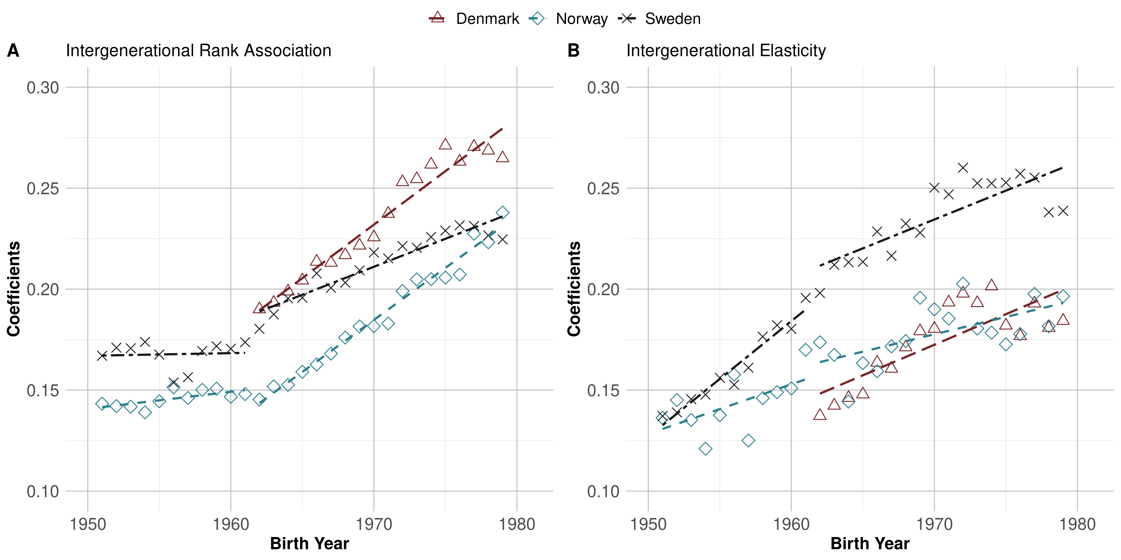
Figure B2: Estimates of IRA and IGE in Labor Income.

Notes: Panel A depicts intergenerational rank associations (eq. 1) between parents and children for Sweden, Norway and Denmark and by birth year of the child. Panel B shows intergenerational income elasticities, i.e. correlations in log income between parent and child pairs (with zero incomes excluded from analysis). Parental income averaged over child ages 17-19, and child income averaged over ages 35-37 in all estimates. “Birth Year” refers to birth year of the child in each parent-child pair.

Notes: Each panel depicts intergenerational rank associations (eq. 1) between parents and children, for each country and by birth year of the child. Panel A shows estimates of the main specification: labor earnings. In panel B, total factor (gross) income is used, and panel C depicts net-of-tax (disposable) income. Parental income averaged over child ages 17-19, and child income averaged over ages 35-37 in all estimates. “Birth Year” refers to birth year of the child in each parent-child pair.

Notes: Each panel depicts intergenerational rank associations (eq. 1) between parents and children, for each country and by birth year of the child. Panel A shows estimates of the main specification: Average income at child ages 35-37. In panel B, child income is measured at ages 31-33, and in panel C, it is measured at ages 39-41. Parental income averaged over child ages 17-19 in all estimations. “Birth Year” refers to birth year of the child in each parent-child pair.

Notes: The figure depicts estimates of the intergenerational rank association in household income between parents and children, for each country and by birth year of the child. Household income is defined following Chetty et al. (2014a), where household income in the offspring generation is the sum of the child and the child’s spouses income. Household income in the parent generation is defined as the sum of the mother and fathers income (incl. their respective spouses) divided by two.

Notes: This figure shows IRA coefficients by birth year of the child, when removing non-participants from the sample. Panel A shows the baseline estimates on the full sample; Panel B removes non-participants of the child generation; Panel C removes non-participants of the child and parent generations. “Participation” is determined by an indicator variable for having annual labor earnings exceeding 10,000 USD in a year. Parental income averaged over child ages 17-19 in all estimations; child income measured as the average over ages 35-37. “Birth Year” refers to birth year of the child in each parent-child pair.

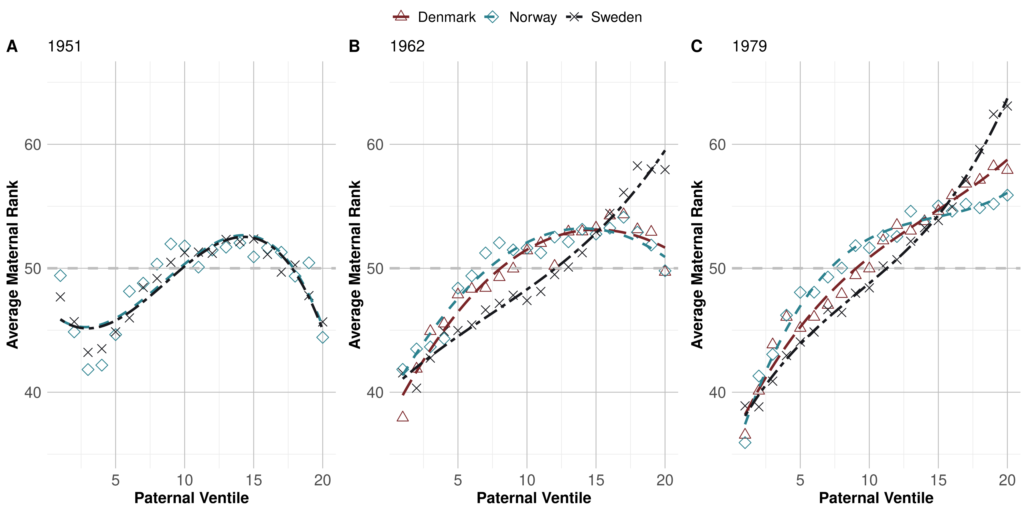
Figure B7: Average Maternal Income Percentile Rank by Paternal Income Ventile.

Notes: The three panels show the average maternal income rank of mothers with children in the same birth cohort, by paternal (within parental pairs) income ventile. Each panel depicts these measures separately by country; for birth cohorts 1951 in Panel A; birth cohort 1962 in Panel B, and birth cohort 1979 in Panel C. The fitted lines are estimated with local polynomial (third order) regressions.

Figure B8: Change in Average Income Rank and Education within Occupation Groups, across Birth Cohorts.

Notes: The figure shows the years of education relative to the mean in a given time period on the x-axis and the mean income rank of mothers in a respective occupation on the y-axis. The left panel provides the relationship between occupations educational level and mean income rank for Norway, while the right panel provides equivalent results for Sweden.

Notes: The figure plots the average years of education within an occupational group (a proxy for the skill level of the occupation) against the change in the share of fathers with a job in that occupational group, from one group of birth cohorts to another. Each dot represents an occupational group, and the size of the dot represents the group size. Purple (filled) circles denote the change from father of the 1951-1955 birth cohorts to father of the 1961-1965 birth cohorts; orange (hollow) circles denote 1961-1965 to 1975-1979. Average years of education calculated in 1975-1979. Dashed lines represent the OLS fitted line between change in occupational share and average years of education, weighted by occupational size; purple for 1951-1965 and orange for 1961-1979. Left panel shows Norway, right panel shows Sweden. Occupations are grouped following Appendix Table A2.

Notes: The figure plots the average years of education within an occupational group (a proxy for the skill level of the occupation) against the change in the share of daughters with a job in that occupational group, from one group of birth cohorts to another. Each dot represents an occupational group, and the size of the dot represents the group size. Purple (filled) circles denote the change from daughters of the 1951-1955 birth cohorts to daughters of the 1961-1965 birth cohorts; orange (hollow) circles denote 1961-1965 to 1975-1979. Average years of education calculated in 1975-1979. Dashed lines represent the OLS fitted line between change in occupational share and average years of education, weighted by occupational size; purple for 1951-1965 and orange for 1961-1979. Left panel shows Norway, right panel shows Sweden. Occupations are grouped following Appendix Table A2.

Figure B11: Relative Importance of Maternal Education, Occupation and Income in Mother-Son Correlations in Latent Economic Status.

Notes: The figure plots the contribution of the different proxy variables to the overall estimate following Lubotsky and Wittenberg (2006). We calculate the contribution of proxy variable $j$ for birth cohort $t$ as $\frac{\rho_{jt}b_{jt}}{\beta^{LW}_{t}}$, i.e. as the share of the aggregate in year $t$ coming from proxy variable $j$. The proxy variables depicted are education, income, and occupation. The contribution of occupations is calculated by summing over the ten different occupational group dummies. The left panel depicts results for Norway, while the right panel shows results for Sweden (data for Denmark is not available for this exercise).

Table B1: Summary Statistics Children 1951 - 1979.

	Number of Children			Son Share Zero			Daughter Share Zero
	DK	NO	SE	DK	NO	SE	DK	NO	SE
	(2)	(3)	(4)	(5)	(6)	(7)	(8)	(9)	(10)
1951		53768	101153		0.0218	0.0093		0.0792	0.0109
1952		57474	101048		0.0247	0.0099		0.0780	0.0096
1953		59492	100978		0.0272	0.0083		0.0785	0.0085
1954		59334	96577		0.0276	0.0097		0.0801	0.0084
1955		60253	98415		0.0279	0.0113		0.0767	0.0091
1956		61008	98904		0.0324	0.0147		0.0810	0.0148
1957		60136	97445		0.0306	0.0166		0.0760	0.0151
1958		60152	96016		0.0302	0.0167		0.0697	0.0154
1959		60297	95185		0.0299	0.0179		0.0659	0.0162
1960		59326	92591		0.0295	0.0194		0.0639	0.0168
1961		59948	94567		0.0282	0.0228		0.0595	0.0169
1962	69948	59843	96813	0.0412	0.0299	0.0217	0.0592	0.0583	0.0178
1963	73901	61073	101760	0.0417	0.0298	0.0214	0.0555	0.0567	0.0170
1964	74955	63298	110549	0.0416	0.0253	0.0207	0.0587	0.0471	0.0177
1965	76700	63988	110364	0.0431	0.0256	0.0204	0.0586	0.0414	0.0169
1966	79340	64874	110074	0.0454	0.0236	0.0195	0.0594	0.0403	0.0162
1967	73204	64721	108302	0.0444	0.0226	0.0198	0.0593	0.0405	0.0159
1968	67242	65963	100853	0.0429	0.0242	0.0187	0.0588	0.0369	0.0159
1969	64121	66462	95375	0.0391	0.0235	0.0215	0.0536	0.0332	0.0160
1970	63892	63636	96388	0.0363	0.0226	0.0211	0.0518	0.0318	0.0173
1971	67457	64517	99960	0.0371	0.0226	0.0229	0.0518	0.0265	0.0175
1972	67514	63452	98766	0.0433	0.0221	0.0220	0.0565	0.0240	0.0177
1973	64060	60694	97018	0.0532	0.0230	0.0247	0.0651	0.0247	0.0183
1974	63527	59327	97644	0.0562	0.0222	0.0257	0.0683	0.0250	0.0201
1975	64604	56014	91500	0.0572	0.0232	0.0256	0.0740	0.0259	0.0202
1976	58824	53354	86260	0.0572	0.0263	0.0261	0.0726	0.0273	0.0194
1977	55902	51076	84042	0.0560	0.0102	0.0283	0.0719	0.0104	0.0195
1978	55893	51893	81184	0.0577	0.0107	0.0269	0.0706	0.0117	0.0205
1979	53578	51791	83740	0.0579	0.0111	0.0285	0.0736	0.0113	0.0188

• Notes: The table provides summary statistics for cohort size and the share of individuals with zero incomes in the child generation. Columns (2)-(4) present the cohort size, columns (5)-(7) indicate the share of sons with zero incomes, and columns (8)-(10) indicate the share of daughters with zero incomes. All statistics are displayed separately by county and birth year of the child.

Table B2: Summary Statistics Parents 1951 - 1979.

	Number of Children			Father ID Missing			Father Share Zero			Mother ID Missing			Mother Share Zero
	DK	NO	SE	DK	NO	SE	DK	NO	SE	DK	NO	SE	DK	NO	SE
	(2)	(3)	(4)	(5)	(6)	(7)	(8)	(9)	(10)	(11)	(12)	(13)	(14)	(15)	(16)
1951		53768	101153		3086	2332		0.0292	0.0976		1109	487		0.5128	0.2856
1952		57474	101048		2642	1826		0.0294	0.0868		851	385		0.4782	0.2363
1953		59492	100978		1652	1633		0.0321	0.0847		488	373		0.4432	0.2103
1954		59334	96577		1449	1480		0.0339	0.0837		380	254		0.3622	0.1913
1955		60253	98415		1218	1320		0.0373	0.0795		370	202		0.3202	0.1700
1956		61008	98904		1154	1259		0.0364	0.0782		300	174		0.2771	0.1466
1957		60136	97445		1074	1210		0.0353	0.0740		256	180		0.2422	0.1171
1958		60152	96016		925	1197		0.0340	0.0731		236	134		0.2107	0.1027
1959		60297	95185		833	1080		0.0325	0.0700		185	108		0.1900	0.0828
1960		59326	92591		749	1106		0.0312	0.0716		207	91		0.1729	0.0743
1961		59948	94567		754	859		0.0291	0.0681		180	2		0.1583	0.0644
1962	69948	59843	96813	1315	826	900	0.0460	0.0306	0.0689	212	175	8	0.1618	0.1474	0.0577
1963	73901	61073	101760	1255	780	926	0.0478	0.0315	0.0668	177	155	6	0.1538	0.1381	0.0531
1964	74955	63298	110549	1209	778	972	0.0469	0.0328	0.0664	129	126	4	0.1421	0.1324	0.0472
1965	76700	63988	110364	1082	857	947	0.0460	0.0340	0.0651	117	99	6	0.1314	0.1261	0.0440
1966	79340	64874	110074	937	852	890	0.0437	0.0325	0.0619	86	82	4	0.1170	0.1133	0.0385
1967	73204	64721	108302	779	839	861	0.0424	0.0324	0.0594	59	88	7	0.1117	0.1015	0.0346
1968	67242	65963	100853	341	828	697	0.0419	0.0319	0.0565	12	96	8	0.1046	0.0965	0.0302
1969	64121	66462	95375	305	813	631	0.0439	0.0317	0.0556	$<$10	72	6	0.1047	0.0901	0.0278
1970	63892	63636	96388	306	768	647	0.0461	0.0339	0.0545	11	91	7	0.1033	0.0907	0.0266
1971	67457	64517	99960	288	720	566	0.0460	0.0347	0.0514	$<$10	90	2	0.0990	0.0921	0.0237
1972	67514	63452	98766	305	760	567	0.0490	0.0364	0.0511	$<$10	75	4	0.0993	0.0916	0.0232
1973	64060	60694	97018	314	793	568	0.0516	0.0380	0.0513	$<$10	66	5	0.0962	0.0908	0.0232
1974	63527	59327	97644	294	736	483	0.0532	0.0411	0.0506	$<$10	88	4	0.0914	0.0920	0.0292
1975	64604	56014	91500	326	760	464	0.0564	0.0387	0.0503	$<$10	82	2	0.0928	0.0899	0.0289
1976	58824	53354	86260	310	778	436	0.0566	0.0426	0.0526	$<$10	64	0	0.0971	0.0895	0.0285
1977	55902	51076	84042	288	740	400	0.0568	0.0411	0.0525	$<$10	78	1	0.0948	0.0859	0.0286
1978	55893	51893	81184	280	767	379	0.0563	0.0405	0.0561	$<$10	72	0	0.0883	0.0808	0.0306
1979	53578	51791	83740	290	802	399	0.0560	0.0408	0.0559	$<$10	96	3	0.0861	0.0786	0.0317

• Notes: The table provides summary statistics for cohort size and the share of individuals with zero incomes in the parent generation. Columns (2)-(4) present the cohort size, columns (5)-(7) and (11)-(13) shows the number of observations with missing father ID or mother ID, columns (8)-(10) and (14)-(16) indicates the share of fathers or mothers with zero income. All statistics are displayed separately by country and birth year of the child.

Table B3: IRA Coefficients, Trends and Differences Across Countries and Time.

	1951		1962			1979			Trend 1962-1979			$\Delta$ p-value
IRA Spec.	NO	SE	DK	NO	SE	DK	NO	SE	DK	NO	SE	DK-NO	DK-SE	NO-SE
All	0.156	0.167	0.190	0.170	0.180	0.265	0.234	0.225	0.530	0.379	0.277	0.065	0.004	0.176
									(0.035)	(0.018)	(0.033)
Son-Parent	0.242	0.245	0.225	0.222	0.233	0.280	0.241	0.235	0.360	0.085	0.014	0.000	0.000	0.736
									(0.036)	(0.024)	(0.061)
Daughter-Parent	0.146	0.158	0.197	0.173	0.169	0.276	0.262	0.240	0.592	0.552	0.428	0.363	0.067	0.020
									(0.035)	(0.037)	(0.038)
Son-Father	0.253	0.248	0.220	0.236	0.242	0.241	0.213	0.211	0.139	-0.160	-0.224	0.000	0.000	0.378
									(0.035)	(0.022)	(0.060)
Son-Mother	0.068	0.080	0.098	0.089	0.101	0.198	0.150	0.155	0.619	0.324	0.307	0.000	0.007	0.723
									(0.026)	(0.026)	(0.041)
Daughter-Father	0.137	0.139	0.175	0.144	0.152	0.216	0.195	0.192	0.342	0.325	0.239	0.778	0.570	0.421
									(0.031)	(0.032)	(0.034)
Daughter-Mother	0.073	0.077	0.120	0.119	0.112	0.227	0.221	0.194	0.731	0.607	0.541	0.439	0.181	0.107
									(0.036)	(0.037)	(0.034)

• Notes: Columns (1)-(7) report the IRA coefficients of separated regressions in the years 1951, 1962 and 1979 separately for Denmark, Norway and Sweden. Columns (8)-(10) report the coefficient of the fitted regression lines of country specific regressions of the IRA coefficient on a linear trend for the years 1962 to 1979. The trend coefficients and corresponding standard errors have been multiplied by 100 in order to avoid too many digits after the separator. Columns (11)-(13) report rounded p-values for the null hypothesis that the slopes for the respective countries (see column header) are equal. Robust standard errors are reported in parentheses.

Table B4: IRA Coefficients and Trends - Details (United States).

	Parents	Father		Mother
	Child	Son	Daughter	Son	Daughter
A: Weights
Pooled IRA	0.317***	0.336***	0.195***	0.097***	0.137***
	(0.017)	(.022)	(0.031)	(0.025)	(0.029)
Trend $\times$ 100	0.603***	-0.240	0.980***	0.136	1.047***
	(0.149)	(0.205)	(0.277)	(0.253)	(0.292)
N	5,392	2,272	1,637	2,477	2,205
B: No weights
Pooled IRA	0.335***	0.360***	0.237***	0.107***	.152***
	(0.013)	(0.020)	(0.025)	(0.021)	(0.022)
Trend $\times$ 100	0.449***	-0.263*	0.728***	0.268	0.917***
	(0.118)	(0.178)	(0.229)	(0.202)	(0.213)
N	5,392	2,272	1,637	2,477	2,205
C: SRC sample
Pooled IRA	0.294***	0.327***	0.192***	0.098***	0.126***
	(0.018)	(0.023)	(0.0353)	(0.026)	(0.032)
Trend $\times$ 100	0.433**	-0.393	1.156***	0.180	0.727
	(0.162)	(0.218)	(0.305)	(0.266)	(0.327)
N	2,927	1,583	904	1,497	1,001

• Notes: The table presents estimates of the IRA and linear trends in the IRA separately for different child-parent combinations. Due to the small sample sizes, trends have been estimated directly on the underlying micro data by regressing cohort-specific child ranks on cohort-specific parent ranks interacted with a linear time trend. The trend coefficients and standard errors have been multiplied by 100 in order to avoid too many digits after the separator. Panel A contains estimates for the full PSID sample using provided sample weights, Panel B uses the full sample without weights and Panel C includes estimates on the nationally representative SRC sample. Standard errors are in parentheses. P-values indicated by * $<$ 0.1, ** $<$ 0.05, *** $<$ 0.01.

Table B5: IRA Coefficients and Trends - Age 30 (United States).

	Parents	Father		Mother
	Child	Son	Daughter	Son	Daughter
A: Weights
Pooled IRA	0.327***	0.318***	0.222***	0.120***	0.151***
	(0.015)	(0.022)	(0.026)	(0.025)	(0.027)
Trend $\times$ 100	0.643***	0.133	0.661***	0.610**	0.571**
	(0.129)	(0.193)	(0.220)	(0.239)	(0.262)
N	6,652	2,664	2,109	2,685	2,611
B: No weights
Pooled IRA	0.345***	0.341***	0.263***	0.148***	0.168***
	(0.012)	(0.018)	(0.021)	(0.019)	(0.020)
Trend $\times$ 100	0.457***	0.102	0.510***	0.429**	0.567***
	(0.101)	(0.59)	(0.183)	(0.176)	(0.181)
N	6,652	2,663	2,109	2,686	2,611
C: SRC sample
Pooled IRA	0.303***	0.310***	0.225***	0.097***	0.133***
	(0.016)	(0.023)	(0.028)	(0.027)	(0.030)
Trend $\times$ 100	0.528***	0.020	0.586**	0.661**	0.352
	(0.146)	(0.210)	(0.245)	(0.261)	(0.307)
N	3,451	1,757	1,161	1,460	1,142

• Note: The table presents estimates of the IRA and linear trends in the IRA separately for different child-parent combinations Children’s income is measure at age 30. Due to the small sample sizes, trends have been estimated directly on the underlying micro data by regressing cohort-specific child ranks on cohort-specific parent ranks interacted with a linear time trend. The trend coefficients and standard errors have been multiplied by 100 in order to avoid too many digits after the separator. Panel A contains estimates for the full PSID sample using provided sample weights, Panel B uses the full sample without weights and Panel C includes estimates on the nationally representative SRC sample. Standard errors are in parentheses. P-values indicated by * $<$ 0.1, ** $<$ 0.05, *** $<$ 0.01.

Table B6: PSID Sample Size with Parent-Child Links by Birth Cohort (United States).

		Parents	Father		Mother
Child birth year		Child	Son	Daughter	Son	Daughter
1947		76	27	26	35	39
1948		107	38	39	48	56
1949		143	52	44	73	65
1950		171	57	72	68	99
1951		218	76	81	101	108
1952		193	70	78	88	102
1953		239	87	98	116	117
1954		235	78	96	101	128
1955		267	103	98	122	136
1956		263	86	106	107	147
1957		247	95	85	126	115
1958		220	75	95	95	119
1959		159	79	37	107	46
1960		177	96	34	121	54
1961		105	54	27	62	38
1962		117	50	37	63	53
1963		125	49	41	64	56
1964		100	47	30	56	43
1965		91	42	20	49	40
1966		88	39	17	52	34
1967		95	49	21	60	33
1968		66	32	17	39	26
1969		99	49	32	55	42
1970		87	40	20	50	35
1971		92	40	21	60	32
1972		111	49	22	63	43
1973		107	50	20	65	36
1974		117	51	25	64	48
1975		128	55	36	70	48
1976		132	58	37	63	53
1977		130	66	23	41	21
1978		138	66	34	27	30
1979		179	93	43	29	41
1980		142	65	36	33	26
1981		148	77	30	40	24
1982		120	58	27	26	30
1983		160	74	32	38	42
Total		5,392	2,272	1,637	2,477	2,205

• Notes: The table presents the number of cohort-specific parent-child links that were used to produce the main results from the PSID survey data.

Table B7: Comparison of Trends 1962 - 1979.

		Denmark	Norway	Sweden
Panel A: Son - Father
	IRA	0.1385	-0.1598	-0.2243
		(0.0349)	(0.0222)	(0.0605)
	LW	0.1504	-0.2062	-0.1898
		(0.0239)	(0.0350)	(0.0613)
	Difference	-0.0118	0.0464	-0.0346
		(0.0423)	(0.0414)	(0.0861)
Panel B: Son - Mother
	IRA	0.6186	0.3244	0.3069
		(0.0256)	(0.0262)	(0.0408)
	LW	0.2994	-0.1200	0.0175
		(0.0353)	(0.0273)	(0.0495)
	Difference	0.3192	0.4444	0.2894
		(0.0436)	(0.0379)	(0.0642)
Panel C: Daughter - Father
	IRA	0.3416	0.3247	0.2388
		(0.0309)	(0.0318)	(0.0339)
	LW	0.0658	-0.0385	-0.0897
		(0.0324)	(0.0314)	(0.0201)
	Difference	0.2758	0.3632	0.3285
		(0.0447)	(0.0447)	(0.0394)

• Notes: IRA indicates linear trends estimated through all coefficients of the intergenerational rank association. LW specifies linear trends estimated through all coefficients obtained from applying the Lubotsky-Wittenberg method. The trend coefficients and corresponding standard errors have been multiplied by 100 in order to avoid too many digits after the separator. Difference indicates differences between LW and IRA trends and tests the null-hypothesis of equality in trends between the IRA and LW coefficients. Heteroskedasticity robust standard errors are in parentheses.

Appendix C Calibrating Parameters in Model

Each set of country-cohort model parameters for trend decomposition are — loosely described — calibrated in the following steps:

1. If the cohort is the first cohort of observation for a given country (say, 1951 in Sweden and Norway and 1962 in Denmark), draw a random set of values for the parameters $\psi_{t},\kappa_{t},\alpha_{t},\phi_{t}^{M}$ and $\phi_{t}^{D}$. If the cohort is not the first cohort of observation, initialize the algorithm with the optimal set of parameters from the last cohort associated with the same country. These become the ’search parameters’ until they are replaced by parameters that are likely superior in terms of fitting the true data as outlined in the next steps.

2. Simulate 100,000 parent-child pairs and repeat the following procedure until there is a sufficiently close match between empirical rank associations as outlined in equations (6a)-(6e) and the simulated counterparts:

   1. Compute skills and incomes for all individuals (father, mother, son and daughter) using the set of ’search parameters’ along with randomly drawn values for $x^{k}_{it}$ and $\varepsilon^{k}_{it}$.

   2. Compute rank associations as listed in equations as outlined in equations equations (6a)-(6e) from the simulated data and match them to the associated rank associations as estimated in the real data.

   3. If the convergence criterion is not met, adjust the parameters using a customized variation of gradient descent. These now become the ’search parameters’.

In Figure C1, we illustrate how the implied empirical association between the two types of income in the (calibrated) simulated data compares to the empirical association between the same two incomes as observed in the data. These figures validate the quality of the calibration exercise.

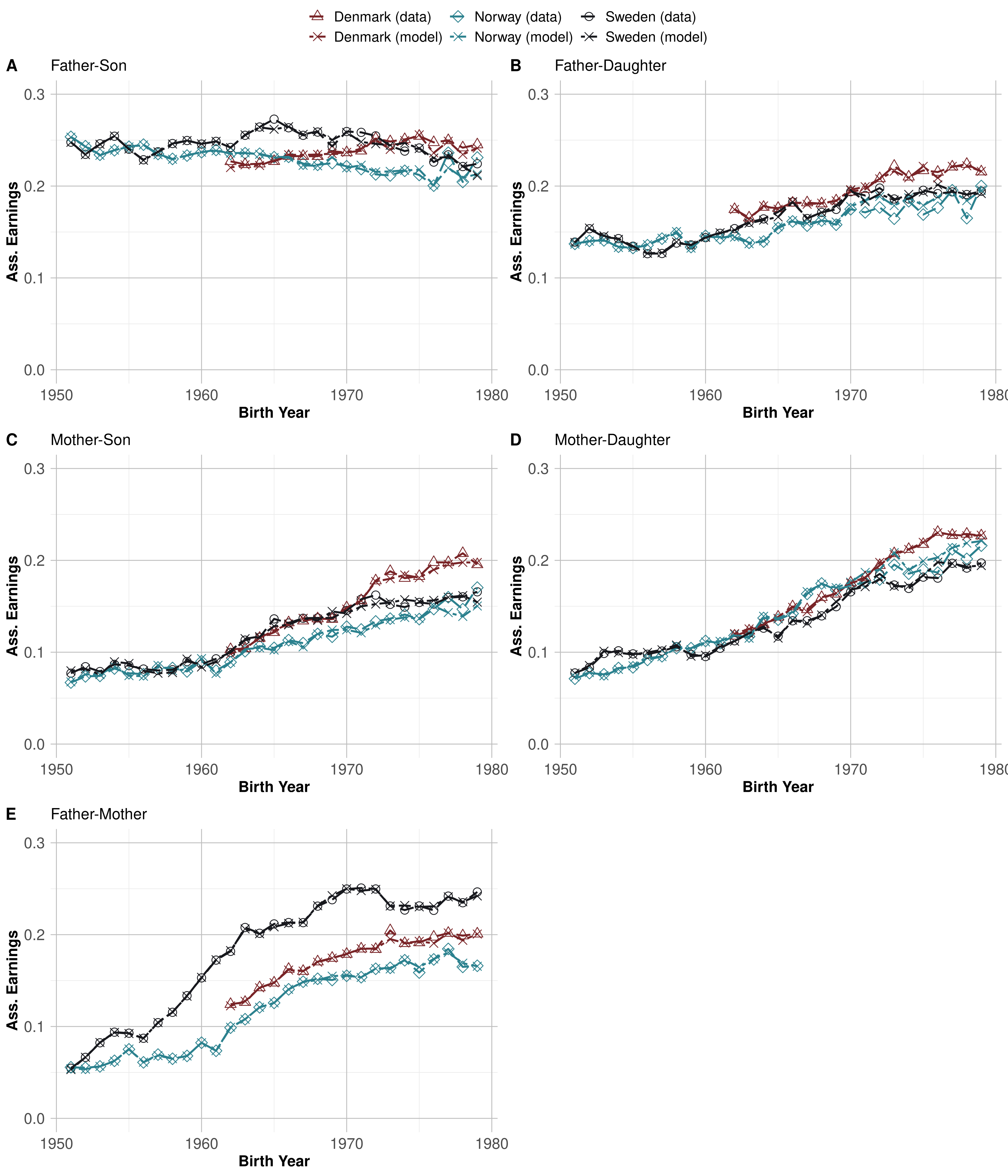
Figure C1: Validation of Calibration Exercise.

Notes: Each panel displays the empirical association between two incomes as observed in the data as well as the implied empirical association between the same two types of income in the simulated data as calibrated in the decomposition model. “Birth Year” refers to birth year of the child in each parent-child pair.

References

- (1)
- Abramitzky et al. (2021) Abramitzky, Ran, Leah Boustan, Elisa Jacome, and Santiago Perez. 2021. “Intergenerational Mobility of Immigrants in the United States over Two Centuries.” American Economic Review, 111(2): 580–608.
- Adermon, Lindahl and Palme (2021) Adermon, Adrian, Mikael Lindahl, and Mårten Palme. 2021. “Dynastic Human Capital, Inequality, and Intergenerational Mobility.” American Economic Review, 111(5): 1523–48.
- Altonji and Dunn (2000) Altonji, Joseph, and Thomas A. Dunn. 2000. “An Intergenerational Model of Wages, Hours, and Earnings.” Journal of Human Resources, 35(2): 221–258.
- Baldacchinoel and Wivel (2020) Baldacchinoel, Godfrey, and Anders Wivel. 2020. Handbook on the Politics of Small States. Cheltenham, Gloucestershire, United Kingdom:Edward Elgar Publishing Limited.
- Becker and Tomes (1979) Becker, Gary S., and Nigel Tomes. 1979. “An Equilibrium Theory of the Distribution of Income and Intergenerational Mobility.” Journal of Political Economy, 87(6): 1153–1189.
- Bhuller, Mogstad and Salvanes (2017) Bhuller, Manudeep, Magne Mogstad, and Kjell G Salvanes. 2017. “Life-Cycle Earnings, Education Premiums, and Internal Rates of Return.” Journal of Labor Economics, 35(4): 993–1030.
- Björklund, Jäntti and Lindquist (2009) Björklund, Anders, Markus Jäntti, and Matthew J Lindquist. 2009. “Family Background and Income During the Rise of the Welfare State: Brother Correlations in Income for Swedish Men Born 1932–1968.” Journal of Public Economics, 93(5-6): 671–680.
- Black, Devereux and Salvanes (2005) Black, Sandra E, Paul J Devereux, and Kjell G Salvanes. 2005. “Why the Apple Doesn’t Fall Far: Understanding Intergenerational Transmission of Human Capital.” American Economic Review, 95(1): 437–449.
- Blanden et al. (2004) Blanden, Jo, Alissa Goodman, Paul Gregg, and Stephen Machin. 2004. “Changes in Intergenerational Mobility in Britain.” Generational Income Mobility in North America and Europe, , ed. MilesEditor Corak, 122–146. Cambridge University Press.
- Blau and Kahn (2017) Blau, Francine D, and Lawrence M Kahn. 2017. “The Gender Wage Gap: Extent, Trends, and Explanations.” Journal of Economic Literature, 55(3): 789–865.
- Blau et al. (2021) Blau, Francine D, Lawrence M Kahn, Nikolai Boboshko, and Matthew L Comey. 2021. “The Impact of Selection into the Labor Force on the Gender Wage Gap.” National Bureau of Economic Research Working Paper 28855.
- Blau, Brummund and Liu (2013) Blau, Francine D., Peter Brummund, and Albert Yung-Hsu Liu. 2013. “Trends in Occupational Segregation by Gender 1970-2009: Adjusting for the Impact of Changes in the Occupational Coding System.” Demography, 50(2): 471–494.
- Brandén and Nybom (2019) Brandén, Gunnar, and Martin Nybom. 2019. “Utvecklingen av intergenerationell rörlighet i Sverige.”
- Brandén, Nybom and Vosters (2023) Brandén, Gunnar, Martin Nybom, and Kelly Vosters. 2023. “Like Mother, Like Child? The Rise of Women’s Intergenerational Income Persistence in Sweden and the United States.”
- Bratberg et al. (2017) Bratberg, Espen, Jonathan Davis, Bhashkar Mazumder, Martin Nybom, Daniel D. Schnitzlein, and Kjell Vaage. 2017. “A Comparison of Intergenerational Mobility Curves in Germany, Norway, Sweden, and the US.” The Scandinavian Journal of Economics, 119(1): 72–101.
- Bratsberg et al. (2023) Bratsberg, Bernt, Simen Markussen, Oddbjørn Raaum, Knut Røed, and Ole Røgeberg. 2023. “Trends in assortative mating and offspring outcomes.” The Economic Journal, 133(651): 928–950.
- Chadwick and Solon (2002) Chadwick, Laura, and Gary Solon. 2002. “Intergenerational Income Mobility Among Daughters.” American Economic Review, 92(1): 335–344.
- Chetty et al. (2014a) Chetty, Raj, Nathaniel Hendren, Patrick Kline, and Emmanuel Saez. 2014a. “Where is the land of opportunity? The geography of intergenerational mobility in the United States.” The Quarterly Journal of Economics, 129(4): 1553–1623.
- Chetty et al. (2014b) Chetty, Raj, Nathaniel Hendren, Patrick Kline, Emmanuel Saez, and Nicholas Turner. 2014b. “Is the United States Still a Land of Opportunity? Recent Trends in Intergenerational Mobility.” The American Economic Review, 104(5): 141–147.
- Collado, Ortuño-Ortín and Stuhler (2022) Collado, M Dolores, Ignacio Ortuño-Ortín, and Jan Stuhler. 2022. “Estimating Intergenerational and Assortative Processes in Extended Family Data.” The Review of Economic Studies, 90(3): 1195–1227.
- Collins and Wanamaker (2022) Collins, William J., and Marianne H. Wanamaker. 2022. “African American Intergenerational Economic Mobility since 1880.” American Economic Journal: Applied Economics, 14(3): 84–117.
- Connolly, Haeck and Lapierre (2019) Connolly, Marie, Catherine Haeck, and David Lapierre. 2019. “Social mobility trends in Canada: Going up the Great Gatsby curve.” Research Group on Human Capital - Working Papers Series Number, , (19-Mar). Working paper (online).
- Connolly, Haeck and Laliberté (2020) Connolly, Marie, Catherine Haeck, and Jean-William P Laliberté. 2020. “Parental Education Mitigates the Rising Transmission of Income between Generations.” In Measuring and Understanding the Distribution and Intra/Inter-Generational Mobility of Income and Wealth. University of Chicago Press.
- Corak (2013) Corak, Miles. 2013. “Income Inequality, Equality of Opportunity, and Intergenerational Mobility.” Journal of Economic Perspectives, 27(3): 79–102.
- Dahl and DeLeire (2008) Dahl, Molly W, and Thomas DeLeire. 2008. “The Association Between Children’s Earnings and Fathers’ Lifetime Earnings: Estimates Using Administrative Data.” University of Wisconsin-Madison, Institute for Research on Poverty.
- Davis and Mazumder (2022) Davis, Jonathan, and Bhashkar Mazumder. 2022. “The Decline in Intergenerational Mobility After 1980.”
- Duncan and Duncan (1955) Duncan, Otis Dudley, and Beverly Duncan. 1955. “A Methodological Analysis of Segregation Indexes.” American Sociological Review, 20(2): 210–217.
- Eika, Mogstad and Zafar (2019) Eika, Lasse, Magne Mogstad, and Basit Zafar. 2019. “Educational assortative mating and household income inequality.” Journal of Political Economy, 127(6): 2795–2835.
- Engzell and Mood (2023) Engzell, Per, and Carina Mood. 2023. “Understanding Patterns and Trends in Income Mobility through Multiverse Analysis.” American Sociological Review, 88(4): 600–626.
- Galassi, Koll and Mayr (2021) Galassi, Gabriela, David Koll, and Lukas Mayr. 2021. “The Intergenerational Correlation of Employment.” University of Bonn and University of Mannheim, Germany CRC TR 224 Discussion Paper Series.
- Goldin (2014) Goldin, Claudia. 2014. “A Grand Gender Convergence: Its Last Chapter.” American Economic Review, 104(4): 1091–1119.
- Grönqvist, Öckert and Vlachos (2017) Grönqvist, Erik, Björn Öckert, and Jonas Vlachos. 2017. “The Intergenerational Transmission of Cognitive and Noncognitive Abilities.” Journal of Human Resources, 52(4): 887–918.
- Harding and Munk (2019) Harding, David J, and Martin D Munk. 2019. “The Decline of Intergenerational Income Mobility in Denmark: Returns to Education, Demographic Change, and Labor Market Experience.” Social Forces, 98(4): 1436–1464.
- Hartley, Lamarche and Ziliak (2022) Hartley, Robert Paul, Carlos Lamarche, and James P Ziliak. 2022. “Welfare reform and the intergenerational transmission of dependence.” Journal of Political Economy, 130(3): 523–565.
- Hertz (2008) Hertz, Tom. 2008. “A group-specific measure of intergenerational persistence.” Economics Letters, 100(3): 415–417.
- Holmlund (2020) Holmlund, Helena. 2020. “How Much Does Marital Sorting Contribute to Intergenerational Socioeconomic Persistence?” Journal of Human Resources.
- Justman, Krush and Millo (2017) Justman, Moshe, Anna Krush, and Hadas Millo. 2017. “The intergenerational elasticity of income in the United States is rising in tandem with income inequality and returns to schooling.” Working Paper. Available from http://www. ecineq. org/ecineq_nyc17 ….
- Jácome, Kuziemko and Naidu (2021) Jácome, Elisa, Ilyana Kuziemko, and Suresh Naidu. 2021. “Mobility for All: Representative Intergenerational Mobility Estimates over the 20th Century.” National Bureau of Economic Research Working Paper 29289.
- Kleven, Landais and Søgaard (2019) Kleven, Henrik, Camille Landais, and Jakob Egholt Søgaard. 2019. “Children and Gender Inequality: Evidence from Denmark.” American Economic Journal: Applied Economics, 11(4): 181–209.
- Kleven (2014) Kleven, Henrik Jacobsen. 2014. “How Can Scandinavians Tax so Much?” Journal of Economic Perspectives, 28(4): 77–98.
- Lee and Solon (2009) Lee, Chul-In, and Gary Solon. 2009. “Trends in Intergenerational Income Mobility.” The Review of Economics and Statistics, 91(4): 766–772.
- Lubotsky and Wittenberg (2006) Lubotsky, Darren, and Martin Wittenberg. 2006. “Interpretation of Regressions with Multiple Proxies.” The Review of Economics and Statistics, 88(3): 549–562.
- Manduca et al. (2020) Manduca, Robert, Maximilian Hell, Adrian Adermon, Jo Blanden, Espen Bratberg, Keun Bok Lee, Stephen Machin, Martin D Munk, Martin Nybom, Yuri Ostrovsky, et al. 2020. “Trends in Absolute Income Mobility in North America and Europe.” IZA Discussion Paper No. 13456.
- Markussen and Røed (2020) Markussen, Simen, and Knut Røed. 2020. “Economic Mobility Under Pressure.” Journal of the European Economic Association, 18(4): 1844–1885.
- Mazumder (2018) Mazumder, Bhashkar. 2018. “Intergenerational Mobility in the United States: What We Have Learned from the PSID.” The ANNALS of the American Academy of Political and Social Science, 680(1): 213–234. PMID: 31666747.
- Meghir and Palme (2005) Meghir, Costas, and Mårten Palme. 2005. “Educational Reform, Ability, and Family background.” American Economic Review, 95(1): 414–424.
- Nybom and Stuhler (2016) Nybom, Martin, and Jan Stuhler. 2016. “Heterogeneous Income Profiles and Lifecycle Bias in Intergenerational Mobility Estimation.” Journal of Human Resources, 51(1): 239–268.
- Nybom and Stuhler (2017) Nybom, Martin, and Jan Stuhler. 2017. “Biases in Standard Measures of Intergenerational Income Dependence.” The Journal of Human Resources, 52: 800 – 825.
- OECD (2021) OECD. 2021. “LFS by Sex and Age.” https://stats.oecd.org/Index.aspx?DataSetCode=lfs_sexage_i_r, Accessed: 2021-02-25.
- Olivetti and Petrongolo (2016) Olivetti, Claudia, and Barbara Petrongolo. 2016. “The Evolution of Gender Gaps in Industrialized Countries.” Annual Review of Economics, 8(1): 405–434.
- Olivetti and Paserman (2015) Olivetti, Claudia, and M. Daniele Paserman. 2015. “In the Name of the Son (and the Daughter): Intergenerational Mobility in the United States, 1850-1940.” American Economic Review, 105(8): 2695–2724.
- Pareliussen et al. (2018) Pareliussen, Jon Kristian, Mikkel Hermansen, Christophe André, and Orsetta Causa. 2018. “Income Inequality in the Nordics from an OECD Perspective.” Nordic Economic Policy Review, 17–57.
- Pekkala and Lucas (2007) Pekkala, Sari, and Robert EB Lucas. 2007. “Differences across cohorts in Finnish intergenerational income mobility.” Industrial Relations: A Journal of Economy and Society, 46(1): 81–111.
- Pekkarinen, Salvanes and Sarvimäki (2017) Pekkarinen, Tuomas, Kjell G Salvanes, and Matti Sarvimäki. 2017. “The Evolution of Social Mobility: Norway During the Twentieth Century.” The Scandinavian Journal of Economics, 119(1): 5–33.
- Ruhm (1998) Ruhm, Christopher J. 1998. “The Economic Consequences of Parental Leave Mandates: Lessons from Europe.” The Quarterly Journal of Economics, 113(1): 285–317.
- Selin (2014) Selin, Håkan. 2014. “The Rise in Female Employment and the Role of Tax Incentives. An Empirical Analysis of the Swedish Individual Tax Reform of 1971.” International Tax and Public Finance, 21(5): 894–922.
- Søgaard (2018) Søgaard, Jakob Egholt. 2018. “Top Incomes in Scandinavia – Recent Developments and the Role of Capital Income.” Nordic Economic Policy Review 2018: Increasing Income Inequality in the Nordics, 66–94.
- Solon (1999) Solon, Gary. 1999. “Chapter 29 - Intergenerational Mobility in the Labor Market.” In . Vol. 3 of Handbook of Labor Economics, , ed. Orley C. Ashenfelter and David Card, 1761–1800. Elsevier.
- Solon (2002) Solon, Gary. 2002. “Cross-Country Differences in Intergenerational Earnings Mobility.” Journal of Economic Perspectives, 16(3): 59–66.
- Solon (2004) Solon, Gary. 2004. “A Model of Intergenerational Mobility Variation Over Time and Place.” Generational Income Mobility in North America and Europe, , ed. MilesEditor Corak, 38–47. Cambridge University Press.
- Song et al. (2020) Song, Xi, Catherine G. Massey, Karen A. Rolf, Joseph P. Ferrie, Jonathan L. Rothbaum, and Yu Xie. 2020. “Long-term decline in intergenerational mobility in the United States since the 1850s.” Proceedings of the National Academy of Sciences, 117(1): 251–258.
- Vosters (2018) Vosters, Kelly. 2018. “Is the Simple Law of Mobility Really a Law? Testing Clark’s Hypothesis.” The Economic Journal, 128(612): F404–F421.
- Vosters and Nybom (2017) Vosters, Kelly, and Martin Nybom. 2017. “Intergenerational Persistence in Latent Socioeconomic Status: Evidence from Sweden and the United States.” Journal of Labor Economics, 35(3): 869–901.