ProxyFormer: Proxy Alignment Assisted Point Cloud Completion with Missing Part Sensitive Transformer

Abstract

Problems such as equipment defects or limited viewpoints will lead the captured point clouds to be incomplete. Therefore, recovering the complete point clouds from the partial ones plays an vital role in many practical tasks, and one of the keys lies in the prediction of the missing part. In this paper, we propose a novel point cloud completion approach namely ProxyFormer that divides point clouds into existing (input) and missing (to be predicted) parts and each part communicates information through its proxies. Specifically, we fuse information into point proxy via feature and position extractor, and generate features for missing point proxies from the features of existing point proxies. Then, in order to better perceive the position of missing points, we design a missing part sensitive transformer, which converts random normal distribution into reasonable position information, and uses proxy alignment to refine the missing proxies. It makes the predicted point proxies more sensitive to the features and positions of the missing part, and thus make these proxies more suitable for subsequent coarse-to-fine processes. Experimental results show that our method outperforms state-of-the-art completion networks on several benchmark datasets and has the fastest inference speed. Code is available at https://github.com/I2-Multimedia-Lab/ProxyFormer.

1 Introduction

3D data is used in many different fields, including autonomous driving, robotics, remote sensing, and more [5, 47, 12, 17, 14]. Point cloud has a very uniform structure, which avoids the irregularity and complexity of composition. However, in practical applications, due to the occlusion of objects, the difference in the reflectivity of the target surface material, and the limitation of the resolution and viewing angle of the visual sensor, the collected point cloud data is often incomplete. The resultant missing geometric and semantic information will affect the subsequent 3D tasks [30]. Therefore, how to use a limited amount of incomplete data to complete point cloud and restore the original shape has become a hot research topic, and is of great significance to downstream tasks [38, 4, 3, 10, 43, 19].

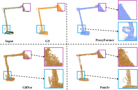
Figure 1: Visual comparison of point cloud completion results. Compared with GRNet [42] and PoinTr [45]. ProxyFormer completely retains the partial input (blue bounding box) and restores the missing part with details (purple bounding box).

With the tremendous success of PointNet [25] and PointNet++ [26], direct processing of 3D coordinates has become the mainstream of point cloud analysis. In recent years, there have been many point cloud completion methods [1, 46, 11, 42, 45, 41, 52], and the emergence of these networks has also greatly promoted the development of this area. Many methods [1, 46, 42] adopt the common encoder-decoder structure, which usually get global feature from the incomplete input by pooling operation and map this feature back to the point space to obtain a complete one. This kind of feature can predict the approximate shape of the complete point cloud. However, there are two drawbacks: (1) The global feature is extracted from partial input and thus lack the ability to represent the details of the missing part; (2) These methods discard the original incomplete point cloud and regenerate the complete shape after extracting features, which will cause the shape of the original part to deform to a certain extent. Methods like [11, 45] attempt to predict the missing part separately, but they do not consider the feature connection between the existing and the missing parts, which are still not good solutions to the first drawback. The results of GRNet [42] and PoinTr [45] in Fig. 1 illustrate the existence of these problems. GRNet failed to keep the ring on the light stand while PoinTr incorrectly predicted the straight edge of the lampshade as a curved edge. Besides, some methods [45, 41, 16, 52] are based on the transformer structure and use the attention mechanism for feature correlation calculation. However, this also brings up two other problems: (3) In addition to the feature, the position encoding also has a great influence on the effect of the transformer. Existing transformer-based methods, either directly using 3D coordinates [9, 52] or using MLP to upscale the coordinates [45, 41], the position information of the point cloud cannot be well represented; (4) It also leads to the problem of excessive parameters or calculation. Furthermore, we also note that most of the current supervised methods do not make full use of the known data. During the training process, the point cloud data we can obtain includes incomplete input and Ground Truth (GT). This pair of data can indeed undertake the point cloud completion task well, but in fact, we can obtain a new data through these two data, that is, the missing part of the point cloud, so as to increase our prior knowledge.

In order to solve the above-mentioned problems, we propose a novel point cloud completion network named ProxyFormer, which completely preserves the incomplete input and has better detail recovery capability as shown in Fig. 1. Firstly, we design a feature and position extractor to convert the point cloud to proxies, with a particular attention to the representation of point position. Then, we let the proxies of the partial input interact with the generated missing part proxies through a newly proposed missing part sensitive transformer, instead of using the global feature extracted from incomplete input alone as in prior methods. After mapping proxies back to the point space, we splice it with the incomplete input points to 100% preserve the original data. During training, we use the true missing part of the point cloud to increase prior knowledge and for prediction error refinement. Overall, the main contributions of our work are as follows:

• We design a Missing Part Sensitive Transformer, which focuses on the geometry structure and details of the missing part. We also propose a new position encoding method that aggregates both the coordinates and features from neighboring points.

• We introduce Proxy Alignment into the training process. We convert the true missing part into proxies, which are used to enhance the prior knowledge while refining the predicted missing proxies.

• Our proposed method ProxyFormer discards the transformer decoder adopted in most transformer based completion methods such as PointTr, which achieves SOTA performance compared to various baselines while having considerably few parameters and the fastest inference speed in terms of GFLOPs.

2 Related Work

3D shape completion. Traditional shape completion work mainly includes two categories: geometric rule completion [51, 24, 21] and template matching completion [22, 13, 15]. However, these methods require the input to be as complete as possible, and thus are not robust to new objects and environmental noise. VoxelNet [53] attempts to divide the point cloud into voxel grids and applies convolutional neural networks, but the voxelization will lose the details of the point cloud, and the increasing resolution of the voxel grid will significantly increase the memory consumption. Yuan et al. [46] designed PCN, which proposed a coarse-to-fine method based on the PointNet [25] and FoldingNet [44], but its decoder often fails to recover rare geometries of objects such as seat backs with gaps, etc. Therefore, after PCN, many other methods [27, 11, 32, 40] focus on multi-step point cloud generation, which is helpful to recover a final point cloud with fine-grained details. Furthermore, following DGCNN [33], some researchers developed graph-based methods [37, 54, 36] which consider regional geometric details. Although these methods provided better feature extractors and decoders, none of them considered the feature connection between the incomplete input and the missing part, which affects the quality of the completion result. Our proposed ProxyFormer is not limited to the partial input but also incorporates true missing points during training. We generate features separately for the missing part and explore the correlation with the features extracted from the partial input via self-attention.

Transformers. The transformer structure originated in the field of natural language processing, which is proposed by Vaswani et al. [31] and applied to machine translation tasks. Recently, this structure was introduced into point cloud processing tasks due to its advantage in extracting correlated features between points. Guo et al. [9] proposed PCT and optimized the self-attention module, making the transformer structure more suitable for point cloud learning, and achieved good performance in shape classification and part segmentation. Point Transformer [50] designs a vector attention for point cloud feature processing. PointTr [45] and SeedFormer [52] treat the point cloud completion as a set-to-set translation problem that share similar ideas as ProxyFormer. PoinTr designs a geometry-aware block that explicitly simulates local geometric relations to facilitate transformers to use better inductive bias. However, it adopts a transformer encoder-decoder structure for point cloud completion, which results in a large amount of parameters. SeedFormer designs an upsample transformer by extending the transformer structure into a basic operation in point generators that effectively incorporates spatial and semantic relationships between neighboring points. However, the upsample transformer runs throughout its network, resulting in excessive computation. Differently, ProxyFormer discards the transformer decoder to reduce the number of parameters, and modifies the query of transformer to make it more suitable for the prediction of the missing part. In the coarse-to-fine process, we still adopt the Foldingnet [44], which greatly reduces the amount of calculation.

3 Method

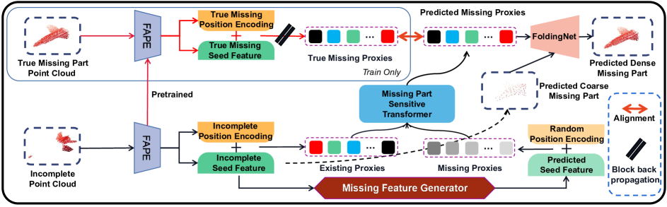
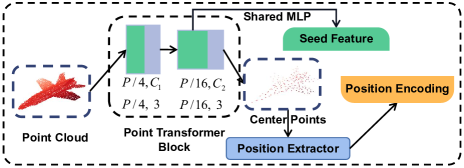
(a) Feature And Position Extractor (FAPE).

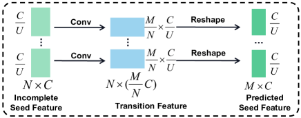
(b) Missing Feature Generator.

Figure 2: The pipeline of ProxyFormer is shown in the upper part. The completion of the point cloud is divided into two steps. First, we simply convert the incomplete seed feature into a predicted coarse missing part. Second, we send the predicted missing proxies and the coarse part into FoldingNet [44] to obtain the predicted dense missing part. True missing part is used for training only so that we block its back-propagation and directly employ the pretrained FAPE on the incomplete point cloud to generate the proxy. (a) The feature and position extractor is applied to obtain seed feature and position encoding which are combined to the so-called proxies. $P$ represents the count of points in the input point cloud. $C_{1}$ and $C_{2}$ is the dimensions of point cloud features. (b) The missing feature generator is used to generate predicted seed feature from incomplete seed feature. $N$ and $M$ means the point count of the incomplete seed feature and predicted seed feature. $C$ means the dimensions of the seed feature and is divided into $U$ groups to speed up operations.

The overall network structure of ProxyFormer is shown in Fig. 2. We will introduce our method in detail as follows.

3.1 Proxy Formation

Proxy introduction. A proxy represents a local region of the point clouds. All the proxies in this paper fuse two information: feature and position. The types of proxies are defined as follows:

• Existing Proxies (EP): It combines incomplete seed feature and incomplete position encoding. (obtained by FAPE).

• Missing Proxies (MP): It combines predicted seed feature and random position encoding. During the training process, MP is also divided into:

  • Predicted Missing Proxies (pre-MP): It is obtained by Missing Part Sensitive Transformer (Sec. 3.2).

  • True Missing Proxies (true-MP): It combines true missing seed feature and true missing position encoding. (obtained by pre-trained FAPE). It is only used for Proxy Alignment (Sec. 3.3).

For clarity, we next explain how to obtain the information these proxies need.

Feature and position extractor (FAPE). For feature extraction, as shown in Fig. 2(a), the point cloud of dimension $\left(P,3\right)$ is sent to point transformer block [50], and the center point cloud of $\left(\frac{P}{16},3\right)$ is obtained by farthest point sampling twice. The feature of $\left(\frac{P}{16},C_{2}\right)$ is obtained through two vector attention calculations [50]. After that, we use a shared MLP to convert the feature to final seed feature.

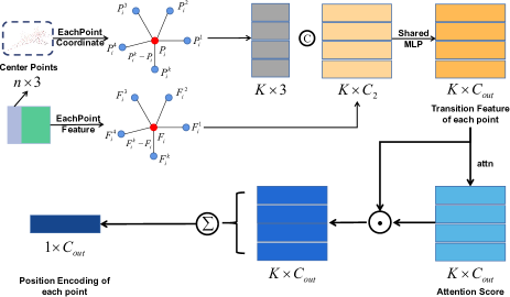
Figure 3: Details of position extractor. $n=\frac{P}{16}$. $K$ is the count of neighbor points. $C_{2}$ and $C_{out}$ are the dimension of point features. $Shared~{}MLP$ means shared multi-layer perceptron and $attn$ means attention score calculation.

For position encoding, we found that directly concatenating the point coordinates with extracted features [26, 49, 33] or simply using MLP to upgrade the three-dimensional coordinates [45] are ineffective. So we design a new position extractor (as shown in Fig. 3) to improve this. The coordinates and features of the center points after feature extraction are used as input. For each point, we take its adjacent $K$ points, and use $\tilde{p}_{i}^{k}=p_{i}^{k}-p_{i}$ to calculate the relative position of the point. $p_{i}^{k}\in{\mathbb{P}=\left\{p_{i}^{1},p_{i}^{2},...,p_{i}^{K}\right\}}$, which means the neighbor point coordinates of $p_{i}$. We also perform neighbor points subtraction in the feature dimension using $\tilde{f}_{i}^{k}=|f_{i}^{k}-f_{i}|$. Similarly, $f_{i}^{k}\in{\mathbb{F}=\left\{f_{i}^{1},f_{i}^{2},...,f_{i}^{K}\right\}}$, which means the neighbor point features of $p_{i}$. After that, we get the coordinate information of $K\times 3$ and the feature information of $K\times C_{2}$. Then we concatenate them and transform feature from $K\times(3+C_{2})$ to $K\times C_{out}$ (the transition feature ${TF}_{i}^{k}$ for each neighboring point) using a shared MLP. After obtaining ${TF}_{i}^{k}$, we use attention mechanism to learn a unique attention score for each channel of point features and then aggregate them. The attention score is calculated and channel-wise multiplied with the feature and summed to obtain the final $PE$ (i.e. position encoding) of each point. This process can be represented by Eq. (1).

$$\begin{aligned} PE=\sum_{k=1}^{K}\left(attn\left(\left\{{TF}_{i}^{k}\right\}\right)\cdot\left\{{TF}_{i}^{k}\right\}\right)\end{aligned}~{},$$ (1)

where $\left\{{TF}_{i}^{k}\right\}$ is the set of transition feature of $K$-neighbor points and $attn()$ is a shared function (per-point MLPs) with learnable weights $W_{attn}$.

Incomplete point cloud and true missing part point cloud are sent into FAPE to get EP and true-MP, and the imcomplete seed feature of EP is used to predict coarse missing part at the same time.

3.2 Missing Part Sensitive Transformer

Usually, query, key and value come from the same input. Many methods [45, 41, 52] attempt to modify the source of value to adapt to the specific tasks (the left part of Fig. 4). Differently, we change the query source, taking the MP with random position encoding as query conditions, to maximally mine the representation of the missing part from the features and positions of existing proxies via self-attention mechanism.

In order to change the query source to MP, we propose a Missing Feature Generator, which is specially used to learn the missing part features from the existing features. The generation process is shown in Fig. 2(b). Specifically, incomplete seed feature of $N\times C$ is used as input, and the $C$-dimensional channels are divided into $U$ equal length groups. Then, the change dimension of the convolution is determined by the point number $M$ of the predicted coarse missing part, which means that we convert each $\frac{C}{U}$ to $\frac{M}{N}\times\frac{C}{U}$. Lastly, we transform the transition feature into predicted seed feature of $M\times C$ through the reshape operation. All channel groups use convolutional layers with shared parameters, reducing the amount of parameters and computation. Predicted missing feature is added with random position encoding to get MP.

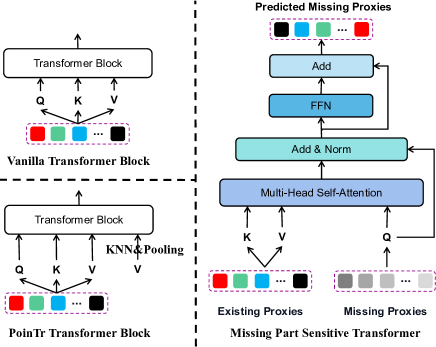
Figure 4: Details of Missing Part Sensitive Transformer. Compared with vanilla transformer block and PoinTr transformer block, we change the source of query to make it more suitable for the prediction of the missing part.

In Sec. 3.1, we have obtained EP and true-MP, and through the missing feature generator described above, we have obtained MP. Then we design a Missing Part Sensitive Transformer to further explore their relationship and learn the representation of the missing points for subsequent completion work. Its structure is illustrated in Fig. 4, which receives EP and MP as input and outputs pre-MP. EP is a matrix $\mathbb{E}$ of $N\times C$, and MP is a matrix $\mathbb{M}$ of $M\times C$. Output pre-MP is a matrix $\mathbb{P}$ of $M\times C$.

We use multi-head self-attention mechanism and add residual connections to obtain pre-MP:

$$\begin{gathered}T=\mu\left(Q+\xi(Q,K,V)\right)~{},\\ \emph{\text{pre-MP}}=\sigma(T)+T~{},\end{gathered}$$ (2)

where $Q=\mathbb{M}\times W^{Q}$, $K=\mathbb{E}\times W^{KV}$, $V=\mathbb{E}\times W^{KV}$. $\mu$ means layer normalization. $\xi$ means multi-head attention calculation. $\sigma$ means feed forward network. The attention of each head is calculated with $Q_{i}$, $K_{i}$, $V_{i}$ on head $i$:

$$\begin{gathered}attn_{i}=softmax\left(\frac{Q_{i}\left(K_{i}\right)^{T}}{\sqrt{d_{k}}}\right)V_{i}\end{gathered}~{}.$$ (3)

This method predicts the proxies of the missing points, which not only discovers feature associations between missing and existing parts, but also converts random positions into meaningful position information. The pre-MP is next used for proxy alignment with true-MP.

3.3 Proxy Alignment

In this subsection, we describe the Proxy Alignment strategy and how this operation assists us in the point cloud completion task.

The detailed computational graph of ProxyFormer is plotted in Fig. 5. Therefore, pre-MP and true-MP can be formulated as:

$$\begin{gathered}\emph{\text{pre-MP}}=T\left({PE}_{R}\oplus\theta\left(\omega\left(C_{i}\right)\right)\right)\\ \emph{\text{true-MP}}={PE}_{T}\oplus\omega\left(C_{m}\right)\end{gathered}~{}.$$ (4)

In order to refine the prediction error in pre-MP, the proxy alignment constraint is imposed on the model, which can be formulated as:

$$\begin{gathered}l_{p}=MSE\left(\emph{\text{pre-MP}},\emph{\text{true-MP}}\right)\end{gathered}~{},$$ (5)

where $l_{p}$ means the alignment loss that we will apply to our training loss (Sec. 3.4) and $MSE$ means the mean squared error. After correcting the pre-MP, it is used as a feature and sent to FoldingNet [44] for coarse-to-fine conversion, and then combined with the previously predicted coarse missing part to obtain the dense missing part.

3.4 Training Loss

Chamfer Distance. We use the average Chamfer Distance(CD) [6] as the first type of our completion loss.

proxy alignment Loss. We use the $MSE$ loss between pre-MP and true-MP as the second type of loss.

To sum up, as shown in Fig. 5, the loss used in this paper consists three parts: (1). $l_{c1}$, the CD between the predicted coarse missing part $C_{pcm}$ and the true center point $C_{tcm}$ of the missing part; (2). $l_{c2}$, the CD between the predicted complete point cloud $C_{pc}$ and the GT $C_{gt}$; (3) $l_{p}$, the alignment loss between pre-MP and ture-MP. We use the weighted sum of these three terms for network training (we set $\gamma$ to $1.5$ in experiments):

$$\begin{gathered}L=l_{c1}+l_{c2}+\gamma l_{p}\end{gathered}~{}.$$ (6)

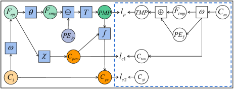
Figure 5: The computational graph for ProxyFormer. The part framed by the blue dotted line is used for training only. For the left part, we input incomplete point cloud $C_{i}$ and use FAPE ($\omega$) to get feature $F_{ep}$ in EP. $F_{ep}$ is not only sent to a linear projection layer $\chi$ to generate predicted coarse missing part $C_{pcm}$, but also sent to missing feature generator ($\theta$) to generate feature $F_{rmp}$. $F_{rmp}$ is added ($\oplus$) with random position distribution ${PE}_{R}$ and sent to missing part sensitive transformer ($T$) to get pre-MP. Then pre-MP and $C_{pcm}$ are sent to FoldingNet ($f$), and the result is spliced with input $C_{i}$ to form predicted complete point cloud $C_{pc}$. For the right part, we input true missing part point cloud $C_{m}$ and use the same FAPE ($\omega$) to get feature $F_{tmp}$ and position ${PE}_{T}$ in true-MP. pre-MP is aligned with true-MP for correcting deviation values. We also retain the center point $C_{tcm}$ obtained after $C_{m}$ is downsampled by FAPE. $l_{p}$, $l_{c1}$ and $l_{c2}$ are the losses we use, which will be detailed in the next subsection.

4 Experiments

In this section, we use ProxyFormer for two common point cloud completion benchmarks PCN [46] and KITTI [7] to evaluate the completion ability of the network, and then we also train and test on two other datasets, ShapeNet-55 and ShapeNet-34 proposed by PoinTr [45]. Finally, through ablation experiments, we demonstrate the effectiveness of each module in the proposed ProxyFormer.

4.1 Point Cloud Completeion on PCN Dataset

Dataset and evaluation metric. The PCN dataset [46] is created from ShapeNet dataset [2], including eight categories with a total of 30974 CAD models. When preparing the data, we use missing part extractor to extract the missing part of the point cloud from the complete point cloud and then downsample it to 3584 points as the true missing part (This process is described in detail in the supplementary material).

We use the L1 CD to evaluate the results of each methods. In addition, We also use density-aware chamfer distance (DCD) [39] as a quantitative evaluation criterion, which can retain the measurement ability similar to CD but also better judge the visual effect of the result.

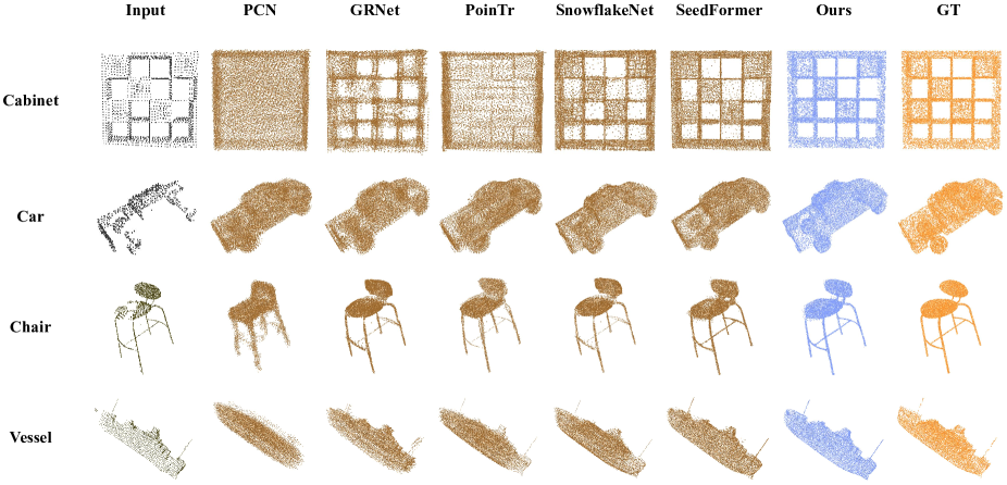
Figure 6: The visualization results of each method on the PCN dataset, showing Cabinet, Car, Chair and Vessel from top to bottom.

Quantiative comparison. According to the results in Table 1, on the PCN dataset, our method has substantially surpassed PoinTr [45] and reaches lowest CD in the cabinet, car, sofa and table categories. Further, as can be seen from the DCD shown in Table 2, our method outperforms state-of-the-art in all the categories, which means that our method is more able to take into account the rationality of shape and distribution density while complementing the object.

Table 1: Quantitative comparison of PCN dataset. Point resolutions for the output and GT are 16384. For CD, lower is better.

Methods	Chamfer Distance($10^{-3}$)
	Air	Cab	Car	Cha	Lam	Sof	Tab	Ves	Ave
FoldingNet [44]	9.49	15.80	12.61	15.55	16.41	15.97	13.65	14.99	14.31
TopNet [27]	7.61	13.31	10.90	13.82	14.44	14.78	11.22	11.12	12.15
AtlasNet [8]	6.37	11.94	10.10	12.06	12.37	12.99	10.33	10.61	10.85
PCN [46]	5.50	22.70	10.63	8.70	11.00	11.34	11.68	8.59	9.64
GRNet [42]	6.45	10.37	9.45	9.41	7.96	10.51	8.44	8.04	8.83
CRN [32]	4.79	9.97	8.31	9.49	8.94	10.69	7.81	8.05	8.51
NSFA [48]	4.76	10.18	8.63	8.53	7.03	10.53	7.35	7.48	8.06
PMP-Net [34]	5.65	11.24	9.64	9.51	6.95	10.83	8.72	7.25	8.73
PoinTr [45]	4.75	10.47	8.68	9.39	7.75	10.93	7.78	7.29	8.38
PMP-Net++ [35]	4.39	9.96	8.53	8.09	6.06	9.82	7.17	6.52	7.56
SnowflakeNet [41]	4.29	9.16	8.08	7.89	6.07	9.23	6.55	6.40	7.21
SeedFormer [52]	3.85	9.05	8.06	7.06	5.21	8.85	6.05	5.85	6.74
ProxyFormer(Ours)	4.01	9.01	7.88	7.11	5.35	8.77	6.03	5.98	6.77

Table 2: Quantitative comparison of PCN dataset. Point resolutions for the output and GT are 16384. For DCD, lower is better.

Methods	Density-aware Chamfer Distance
	Air	Cab	Car	Cha	Lam	Sof	Tab	Ves	Ave
GRNet [42]	0.688	0.582	0.610	0.607	0.644	0.622	0.578	0.642	0.622
PoinTr [45]	0.574	0.611	0.630	0.603	0.628	0.669	0.556	0.614	0.611
SnowflakeNet [41]	0.560	0.597	0.603	0.582	0.598	0.633	0.521	0.583	0.585
SeedFormer [52]	0.557	0.592	0.598	0.579	0.585	0.626	0.520	0.605	0.583
ProxyFormer(Ours)	0.555	0.590	0.597	0.571	0.562	0.626	0.518	0.507	0.577

Qualitative comparison. In Fig. 6, we visualize the completion results of different methods on the PCN dataset. Compared with other methods, the results show that our method can perceive the position of the missing points while completing, and reduce the noisy points in the process of refinement. For example, as can be seen from the chair in the third row, except that the chair generated by PCN [46] has been deformed to a large extent, the other methods have successfully recovered the complete chair, but there are many noisy points around it. The chair completed by our method is more visually plausible. In addition, it can be evident from the chair leg and back that the chair completed by our method are more prominent in detail.

4.2 Point Cloud Completion on ShapeNet-55/34

Table 3: Quantitative comparison on ShapeNet-55. For L2 CD $\times 1000$ and DCD, lower is better. For F1-Score@1%, higher is better.

Methods	Table	Chair	Plane	Car	Sofa	CD-S	CD-M	CD-H	DCD-S	DCD-M	DCD-H	CD-Avg	DCD-Avg	F1
FoldingNet [44]	2.53	2.81	1.43	1.98	2.48	2.67	2.66	4.05	-	-	-	3.12	-	0.082
PCN [46]	2.13	2.29	1.02	1.85	2.06	1.94	1.96	4.08	0.570	0.609	0.676	2.66	0.618	0.133
TopNet [27]	2.21	2.53	1.14	2.18	2.36	2.26	2.16	4.30	-	-	-	2.91	-	0.126
PFNet [11]	3.95	4.24	1.81	2.53	3.34	3.83	3.87	7.97	-	-	-	5.22	-	0.339
GRNet [42]	1.63	1.88	1.02	1.64	1.72	1.35	1.71	2.85	0.545	0.581	0.650	1.97	0.592	0.238
PoinTr [45]	0.81	0.95	0.44	0.91	0.79	0.58	0.88	1.79	0.525	0.562	0.637	1.09	0.575	0.464
SeedFormer [52]	0.72	0.81	0.40	0.89	0.71	0.50	0.77	1.49	0.513	0.549	0.612	0.92	0.558	0.472
Ours	0.70	0.83	0.34	0.78	0.69	0.49	0.75	1.55	0.502	0.536	0.608	0.93	0.549	0.483

Table 4: Quantitative comparison on ShapeNet-34. For L2 CD $\times 1000$ and DCD, lower is better. For F1-Score@1%, higher is better.

Methods	34 seen categories									21 unseen categories
	CD-S	CD-M	CD-H	DCD-S	DCD-M	DCD-H	CD-Avg	DCD-Avg	F1	CD-S	CD-M	CD-H	DCD-S	DCD-M	DCD-H	CD-Avg	DCD-Avg	F1
FoldingNet	1.86	1.81	3.38	-	-	-	2.35	-	0.139	2.76	2.74	5.36	-	-	-	3.62	-	0.095
PCN	1.87	1.81	2.97	0.571	0.617	0.683	2.22	0.624	0.150	3.17	3.08	5.29	0.601	0.638	0.692	3.85	0.644	0.101
TopNet	1.77	1.61	3.54	-	-	-	2.31	-	0.171	2.62	2.43	5.44	-	-	-	3.50	-	0.121
PFNet	3.16	3.19	7.71	-	-	-	4.68	-	0.347	5.29	5.87	13.33	-	-	-	8.16	-	0.322
GRNet	1.26	1.39	2.57	0.550	0.594	0.656	1.74	0.600	0.251	1.85	2.25	4.87	0.583	0.623	0.670	2.99	0.625	0.216
PoinTr	0.76	1.05	1.88	0.533	0.570	0.622	1.23	0.575	0.421	1.04	1.67	3.44	0.558	0.608	0.647	2.05	0.604	0.384
SeedFormer	0.48	0.70	1.30	0.513	0.561	0.608	0.83	0.561	0.452	0.61	1.07	2.35	0.541	0.587	0.629	1.34	0.586	0.402
Ours	0.44	0.67	1.33	0.506	0.557	0.606	0.81	0.556	0.466	0.60	1.13	2.54	0.538	0.584	0.627	1.42	0.583	0.415

Dataset and evaluation metric. We also evaluate our model on two other datasets, ShapeNet-55 and ShapeNet-34, proposed in PoinTr [45]. In the two datasets, the input incomplete point cloud has 2048 points, and the complete point cloud contains 8192 points. Like [45], we randomly select a viewpoint during training, and select a value from 2048 to 6144 to delete the corresponding points (25% to 75% of the complete point cloud), and then downsample the remaining points to 2048, as the input for model training. For the deleted part, we downsample it to 1536 points, as the true missing part. During testing, we choose 8 fixed viewpoints, and set the count of incomplete points to 2048, 4096 or 6144 (25%, 50% or 75% of the complete point cloud), corresponding to three difficulty levels (simple, moderate and hard) during testing.

We use L2 CD, DCD and F-Score as evaluation metrics.

Quantitative comparison. We list the quantitative performance of several methods on ShapeNet-55 and ShapeNet-34 in Tables 3 and 4, respectively. We use CD-S, CD-M and CD-H to represent the CD results under the simple, moderate and hard settings. The same goes for DCD (the short line in the table indicates that the DCD value of this method is not competitive). It can be seen from Table 3 that ProxyFormer achieves the best performance on most listed categories and make lowest CD on simple and moderate settings. As for DCD, our method has the lowest values on all the three settings, which proves that the objects completed by ProxyFormer have the closest density distribution to GT. In terms of F1-Score, our method improved by 2.3% compared with SeedFormer, reaching the highest value. Similarly, in Table 4, we can also see that the three indicators of CD, DCD and F1-Score of ProxyFormer in the 34 visible categories have greatly exceeded PoinTr [45], and in all the three settings, we still get the lowest DCD. Among 21 unseen categories, ProxyFormer also make the lowest DCD and the highest F1-Score, which demonstrates the generalization performance of ProxyFormer. (More results will be presented in the supplementary material)

4.3 Point Cloud Completion on KITTI

Dataset and evaluation metric. To further evaluate our proposed model, we test it on the real-scanned dataset KITTI [7], which have no GT values as a reference, and some of the data are very sparse.

We use Fidelity Distance and Minimal Matching Distance (MMD) as evaluation metric.

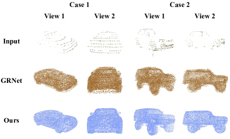
Figure 7: The visualization results on KITTI dataset. To better show the effect of completion, we provide two views for each car.

Quantitative and Qualitative comparison. Following GRNet [42], we fine-tune our pretrained model on ShapeNetCars (cars in the ShapeNet dataset) and evaluate it on the KITTI dataset, and the evaluation results are shown in Table 5. From this we can see that our method achieves the state-of-the-art on MMD (since both our method and PoinTr[45] merge input into the final result, the Fidelity Distance is both $0$). As shown in Fig. LABEL:Fig.11., our method performs well on such real scan data, and even if the input point cloud is very sparse, our method can restore its shape well, and by comparing with the results of GRNet, it can be seen that the point cloud generated by ProxyFormer is softer, with less noisy points, and is more ornamental.

Table 5: Quantitative comparison on KITTI dataset. For Fidelity Distance and Minimal Matching Distance (MMD), lower is better.

	AtlasNet [8]	PCN [46]	FoldingNet [44]	TopNet [27]	MSN [18]	NSFA [48]	CRN [32]	GRNet [42]	PoinTr [45]	SeedFormer [52]	Ours
Fidelity	1.759	2.235	7.467	5.354	0.434	1.281	1.023	0.816	0.000	0.151	0.000
MMD	2.108	1.366	0.537	0.636	2.259	0.891	0.872	0.568	0.526	0.516	0.508

4.4 Ablation Studies

In this subsection, we conduct ablation experiments for ProxyFormer on the PCN dataset [46] to demonstrate the effectiveness of our proposed components.

Model Design Analysis. The results of removing each component are listed in Table 6. The baseline model A only uses Point Transformer for feature extraction, and then send this feature into vanilla transformer encoder to get the feature for FoldingNet. We then add the position extractor to extract the position encoding for each point (Model B). It can be seen that the position extractor we designed reduces the CD of the baseline by $1.06$. After using missing part sensitive transformer for missing proxies prediction (Model C), we can observe that the CD drops significantly to $7.74$. When proxy alignment comes into play, the CD value drops a further $0.97$.

Table 6: Ablation study of each component. We add components including Position Extractor (PE), Missing Part Sensitive Transformer (Sensitive) and Proxy Alignment (PA) step by step.

Model	PE	Sensitive	PA	CD
A				11.08
B	✓			10.02
C	✓	✓		7.74
D	✓	✓	✓	6.77

After conducting ablation experiments on the proposed module, we further demonstrate the irreplaceability of position extractor through one more ablation experiments.

Position Extractor. Our position extractor can synthesize the coordinates and feature information of the point cloud to more accurately represent the correlation and similarity between points. In this experiment, we compare our proposed position encoding method with two method: (1) directly use 3D coordinates as position encoding; (2) MLP-style position encoding method. which performs a simple upscaling operation on the 3D coordinates of the point cloud to form position encoding. The results in Table 7 show that the direct use of 3D coordinates provides very limited position information and MLP cannot extract the positional of the point cloud well. Our proposed position encoding method can perceive the geometric structure of the point cloud well, and in this process, it is optimal to fuse the coordinates and feature information of 16 nearby points.

More ablation experiments and analysis will be given in the supplementary material.

Table 7: Ablation study of Position Extractor of FAPE Module.

Methods	Attempts	CD-Avg
w/o Position Extractor	w/ 3D coordinates	9.63
	w/ MLP	7.83
w/ Position Extractor	num of neighbor = 8	6.86
	num of neighbor = 16	6.77
	num of neighbor = 32	6.92

4.5 Complexity Analysis

Our method achieves the best performance on many metrics on PCN dataset, ShapeNet-55, ShapeNet-34 and KITTI datasets. In Table 8, we list the number of parameters (Params), theoretical computation cost (FLOPs), the average chamfer distances (CD-Avg) and the average density-aware chamfer distances (DCD-Avg) of our method and other six methods. It can be seen that our method can obtain the lowest DCD-Avg while having the smallest FLOPs, and it is the second best only a litter inferior to SeedFormer [52] in terms of CD. Since the transformer decoder part was no longer needed in ProxyFormer, the number of parameters is also greatly reduced compared to PoinTr [45], which also shows that our method can better balance computational cost and performance.

Table 8: Complexity analysis. We show the the number of parameter (Params) and FLOPs of our method and six existing methods. We also provide the distance metrics CD-Avg and DCD-Avg on PCN dataset.

Methods	Params	FLOPs	CD-Avg	DCD-Avg
FoldingNet [44]	2.41M	27.65G	14.31	0.688
PCN [46]	6.84M	14.69G	9.64	0.651
GRNet [42]	76.71M	25.88G	8.83	0.622
PoinTr [45]	30.9M	10.41G	8.38	0.611
SnowflakeNet [41]	19.32M	10.32G	7.21	0.585
SeedFormer [52]	3.20M	29.61G	6.74	0.583
Ours	12.16M	9.88G	6.77	0.577

5 Conclusion

In this paper, we propose a new point cloud completion framework named ProxyFormer, which designs a missing part sensitive transformer to generate missing proxies. We extract feature and position for the missing points and form point proxies. We regularize the distribution of predicted point proxies through proxy alignment, so as to better complete the input partial point clouds. Experiments also show that our method achieves state-of-the-art performance on multiple metrics on several challenging benchmark datasets and has the fastest inference speed.

Appendix A Overview

In this supplementary material, we provide additional information to complement the manuscript. First, we provide the details of missing part extractor in Sec. B. Second, we present additional implementation details and experimental settings of ProxyFormer (Sec. C). At last, we do more ablation studies and visualize more qualitative results of our method on the PCN dataset and ShapeNet-55/34. We also present detailed quantitative results on ShapeNet-55 and ShapeNet-34. (Sec. D).

Appendix B Missing Part Extractor

The given complete point cloud and incomplete point cloud of some point cloud completion common datasets such as PCN are not in the same scale of coordinate systems. So it is not possible to simply use the set difference operation to obtain the missing part. So we design a missing part extractor based on point-to-point and point-to-plane distances [28]. Fig. 8 is a detailed description of the missing part extractor.

Let A and B denote the Ground Truth (GT) and the incomplete point cloud, respectively. Firstly, we use the normal vector estimation method [29] to obtain the normal vector of each point in B. For each point $\bm{p}_{i}$, we assume the covariance matrix $\mathcal{C}$ as follows:

$$\mathcal{C}=\frac{1}{k}\sum_{i=1}^{k}\cdot\left(\bm{p}_{i}-\overline{\bm{p}}\right)\cdot\left(\bm{p}_{i}-\overline{\bm{p}}\right)^{T},$$ (7)

$$\mathcal{C}\cdot\overrightarrow{\mathbf{v}_{j}}=\lambda_{j}\cdot\overrightarrow{\mathbf{v}_{j}},j\in\{0,1,2\}~{}.$$

Here $k$ refers to the $k$ points closest to $\bm{p}_{i}$. $\overline{\bm{p}}$ is the centroid of the nearest neighbor. $\lambda_{j}$ is the $j^{th}$ eigenvalue and $\overrightarrow{\mathbf{v}_{j}}$ is the $j^{th}$ eigenvector. Then, the eigenvector corresponding to the largest eigenvalue is selected and normalized as the normal vector of the point.

Figure 8: The pipeline of Missing Part Extractor. $N$ is the count of points in ground truth and $n$ is the count of points in incomplete input. Firstly, normal vectors are estimated for the incomplete input $\mathbf{B}$. Secondly, the KNN algorithm is used to obtain the index with the shortest distance in $\mathbf{B}$ corresponding to each point in the ground truth $\mathbf{A}$. A set of points $\mathbf{R}$ and a set of normal vectors $\mathbb{N}$ are obtained according to the index. Finally, we use $\mathbf{R}$, $\mathbb{N}$ and $\mathbf{A}$ to calculate the point-to-point distance and the point-to-plane distance. The weighted sum $D$ of these two distances is used for comparison with a pre-defined threshold $0.01$. If the distance is less than or equal to the threshold, the point belongs to the existing part, otherwise it belongs to the missing part.

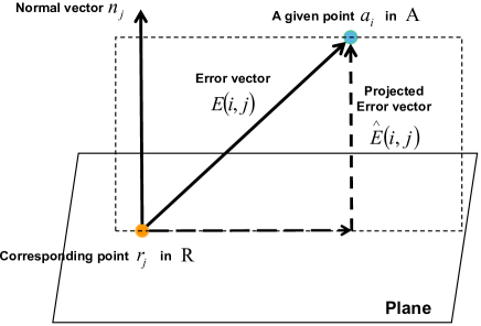
Figure 9: Point-to-point and point-to-plane distance. We use vector calculations to get the two distances. $a_{i}$ is a point in point cloud $\mathbf{A}$ and $r_{j}$ is the corresponding point in $\mathbf{R}$. $n_{j}$ is the normal vector of point $r_{j}$. The error vector $E(i,j)$ is computed by connecting point $r_{j}$ to point $a_{i}$. The projected error vector $\hat{E}\left(i,j\right)$ is the new error vector after $E(i,j)$ is projected along the normal vector $n_{j}$.

After the calculation of the normal vector, the KNN algorithm is used to obtain the index of the corresponding adjacent points between the GT and the incomplete point cloud, which can be expressed as: $idx=KNN\left(\rm{\mathbf{A}},\rm{\mathbf{B}},\rm{K}=1\right)$. According to this index, we go to B to find the points $\bm{b}_{i}$ ($i\in idx$) and normal vectors $\bm{n}_{i}$ ($i\in idx$) of the adjacent points. Here we denote the point cloud composed of $b_{i}$ as $\mathbf{R}$ (it contains $N$ points and the value of each point comes from the incomplete input, but they are one-to-one correspondence with points in GT), and denote the set of normal vectors $n_{i}$ corresponding to each point in the point cloud $\mathbf{R}$ as $\mathbb{N}$.

Then as shown in Fig. 9, we calculate the point-to-point distance and the point-to-plane distance as follows.

(1) For a point $a_{i}$ in point cloud $\mathbf{A}$, i.e., the blue point in the figure, a corresponding point $r_{j}$ in the point cloud $\mathbf{R}$ can be found, i.e., the orange point in the figure. Vice versa.

(2) Similarly, we can get the corresponding normal vector $n_{j}$ from $\mathbb{N}$.

(3) We connect point $r_{j}$ to point $a_{i}$ to calculate an error vector whose length is the point-to-point distance, i.e.,

$$\begin{gathered}D_{a_{i},r_{j}}^{c2c}=||E\left(i,j\right)||_{2}~{}.\end{gathered}$$ (8)

(4) We project the error vector $E\left(i,j\right)$ along the direction of normal vector $n_{j}$ to get another error vector $\hat{E}\left(i,j\right)$ whose length is the point-to-plane distance, i.e.,

$$\begin{gathered}D_{a_{i},r_{j}}^{c2p}=||\hat{E}(i,j)||_{2}=\frac{E(i,j)\cdot n_{j}}{||n_{j}||_{2}}=||E\left(i,j\right)\cdot n_{j}||_{2}~{}.\end{gathered}$$ (9)

(5) We use the weighted sum of the two distances as a comparison condition,

$$\begin{gathered}D=\alpha D_{a_{i},r_{j}}^{c2c}+\beta D_{a_{i},r_{j}}^{c2p}~{},\end{gathered}$$ (10)

where $\alpha=0.2$ and $\beta=0.8$.

We perform the above operations on each point in the GT $\mathbf{A}$. If the calculated distance of the point is less than or equal to the preset threshold of $0.01$, the point is stored in the set of existing parts, otherwise, it is stored in the set of missing parts. This process can be formulated as,

$$\begin{gathered}a_{i}\in\left\{\begin{array}[]{l}Existing~{}part~{}~{}~{}~{}if~{}~{}~{}~{}D<=0.01\\ Missing~{}part~{}~{}~{}~{}~{}~{}~{}~{}~{}~{}~{}~{}~{}~{}~{}else\\ \end{array}\right.~{},\forall a_{i}\in\textbf{A}~{}.\end{gathered}$$ (11)

The missing part is separated from the GT by the above method, and then downsampled to the same number as the incomplete input point for subsequent use. In Fig. 10, we show some results of missing part extractor.

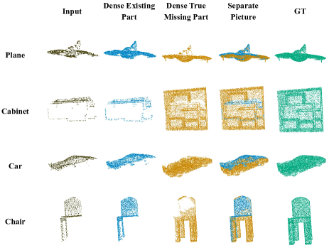
Figure 10: Some results of missing part extractor. From left to right are input, dense existing part, dense missing part, the splicing of the two and GT. From top to bottom are cases in four categories plane, cabinet, car and chair.

Appendix C Implementation Details

In this section, we provide additional implementation details of the proposed ProxyFormer.

C.1 Basic experimental setup

We use Pytorch [23] for our implementation. All network are trained on a single NVIDIA GeForce RTX 3090 graphics card. AdamW optimizer [20] is uesd to train the network with initial learning rate as $5e-4$ and weight decay as $5e-4$. When training on the PCN dataset, we set the batch size to $64$ and train the model for $400$ epochs with the continuous learning rate decay of $0.95$ for every $20$ epochs. When training on ShapeNet-55/34, we set the batch size to $128$ and train the model for $300$ epochs with the continuous learning rate decay of $0.83$ for every $20$ epochs.

C.2 Four types of proxies

There are four types of proxies during training, existing proxies (EP), missing proxies (MP), true missing proxies (true-MP), predicted missing proxies (pre-MP). true-MP is not available during testing. When training on the PCN dataset [46], EP is a $128\times 384$ matrix and MP, true-MP and pre-MP are both $224\times 384$ matrices. When training on the ShapeNet-55/34 [45], EP is a $128\times 384$ matrix and MP, true-MP and pre-MP are both $96\times 384$ matrices.

C.3 Feature and Position Extractor

Feature Extraction. We use farthest point sampling [26] (FPS) to downsample the point cloud and use point transformer [50] (PT) to help exchange information between localized feature vectors. First we use an shared MLP to upscale the 3D coordinates of the point cloud to 32-dim as features. Suppose the set of input point cloud is $P_{i}$, at each downsampling stage: (1) perform farthest point sampling in $P_{i}$ and form a new set $P_{o}$ ($P_{o}\subset P_{i}$); (2) a $k$NN graph is performed on the $P_{i}$ (we use $k=16$ in our experiments); (3) local max pooling is used to aggregate the features of nearby $k$ points to the current center point; (4) enhance features with point transformer block.

On both PCN and ShapeNet-55/34 datasets, the number of incomplete point cloud points input is $P=2048$. Detailed network architecture is as follows:

incomplete input ($2048\times 3$) $\rightarrow$ shared-MLP ($2048\times 3$ to $2048\times 32$) $\rightarrow$ FPS ($2048\times 32$ to $512\times 128$) $\rightarrow$ PT ($512\times 128$ to $512\times 128$) $\rightarrow$ FPS ($512\times 128$ to $128\times 384$) $\rightarrow$ PT ($128\times 384$ to $128\times 384$).

On PCN (ShapeNet-55/34) dataset, the number of missing part points input is $P=3584\textbf{(1536)}$. Bold numbers correspond to the settings on ShapNet-55/34. The process of FAPE is:

missing part ($3584\textbf{(1536)}\times 3$) $\rightarrow$ shared-MLP ($3584\textbf{(1536)}\times 3$ to $3584\textbf{(1536)}\times 32$) $\rightarrow$ FPS ($3584\textbf{(1536)}\times 32$ to $896\textbf{(384)}\times 128$) $\rightarrow$ PT ($896\textbf{(384)}\times 128$ to $896\textbf{(384)}\times 128$) $\rightarrow$ FPS ($896\textbf{(384)}\times 128$ to $224\textbf{(96)}\times 384$) $\rightarrow$ PT ($224\textbf{(96)}\times 384$ to $224\textbf{(96)}\times 384$).

Position Extraction. In order to keep the final position dimension consistent with the feature dimension extracted in the previous step, we set both $C_{2}$ and $C_{out}$ in the main text to $384$. Suppose the set of center points is $P_{c}$ and the final feature of feature extraction is $F_{c}$. Perform $k$-neighbor (we use $k=16$ in our experiments) subtraction ($k$NN-sub) and aggregation ($k$NN-agg) operations on $P_{c}$ and $F_{c}$, respectively.

On both PCN and ShapeNet-55/34 datasets, the number of incomplete center points input is $n=128$. Detailed network architecture is as follows:

$P_{c}$ ($128\times 3$) $\rightarrow$ $k$NN-sub ($128\times 3$ to $128\times 16\times 3$) $\rightarrow$ $k$NN-agg ($128\times 16\times 3$ to $128\times 3$) ,

$F_{c}$ ($128\times 384$) $\rightarrow$ $k$NN-sub ($128\times 384$ to $128\times 16\times 384$) $\rightarrow$ $k$NN-agg ($128\times 16\times 384$ to $128\times 384$) ,

[$P_{c}$, $F_{c}$] ($128\times 387$) $\rightarrow$ shared-MLP ($128\times 387$ to $128\times 384$) .

On PCN (ShapeNet-55/34) dataset, the number of missing part center points input is $n=224\textbf{(96)}$. Bold numbers correspond to the settings on ShapNet-55/34. Detailed network architecture is as follows:

$P_{c}$ ($224\textbf{(96)}\times 3$) $\rightarrow$ $k$NN-sub ($224\textbf{(96)}\times 3$ to $224\textbf{(96)}\times 16\times 3$) $\rightarrow$ $k$NN-agg ($224\textbf{(96)}\times 16\times 3$ to $224\textbf{(96)}\times 3$) ,

$F_{c}$ ($224\textbf{(96)}\times 384$) $\rightarrow$ $k$NN-sub ($224\textbf{(96)}\times 384$ to $224\textbf{(96)}\times 16\times 384$) $\rightarrow$ $k$NN-agg ($224\textbf{(96)}\times 16\times 384$ to $224\textbf{(96)}\times 384$) ,

[$P_{c}$, $F_{c}$] ($224\textbf{(96)}\times 387$) $\rightarrow$ shared-MLP ($224\textbf{(96)}\times 387$ to $128\times 384$) .

Subsequent attention score calculations do not affect the dimension of this feature.

C.4 Missing Part Prediction

In the main text we have mentioned using the incomplete seed feature to generate coarse missing part. When training on PCN dataset, the predicted coarse missing part contains 224 points and the predicted dense missing part contains 14336 points. When training on ShapeNet-55/34, the predicted coarse missing part contains 96 points and the predicted dense missing part contains 6144 points.

C.5 Missing Feature Generator

In Mssing Feature Generator, we set $N$ to $128$ and $M$ to $224$ (on PCN dataset) or $96$ (on ShapeNet-55/34). $C=384$ and we divide the feature dimension equally into $U=16$ groups.

C.6 Missing Part Sensitive Transformer

Like other tansformer-based methods, we stack the missing part sensitive transformer and set its depth to 8.

Multi-Head Self-Attention. This structural design allows each attention mechanism to map to different spaces through Query, Key and Value to learn features. In this way, the different feature parts of each proxy are optimized, so as to make the proxies contain more diverse representations. In all our experiments, we set the number of multi-head attention heads to $8$.

Feed-Forward Network (FFN). Referring to [31] and [45], we set up the feed-forward network as two linear layers with ReLU activation function and dropout.

C.7 The calculation of DCD

Wu et al. [39] study the limitations of CD, believe that CD is not the optimal indicator for evaluating the visual quality of point cloud completion tasks, and proposed the density-aware chamfering distance (DCD), which can retain the measurement ability similar to CD and can also better judge the visual effect of the point cloud completion result. The formula for DCD is as follows:

$$d_{DCD}\left(S_{1},S_{2}\right)=\frac{1}{2}\left(\frac{1}{\left|S_{1}\right|}\sum_{x\in S_{1}}\left(1-\frac{1}{n_{\hat{y}}}e^{-\alpha\|x-\hat{y}\|_{2}}\right)\right)$$ (12)

$$+\frac{1}{2}\left(\frac{1}{\left|S_{2}\right|}\sum_{y\in S_{2}}\left(1-\frac{1}{n_{\hat{x}}}e^{-\alpha\|y-\hat{x}\|_{2}}\right)\right)~{},$$

where $\hat{y}=min_{y\in S_{2}}\|x-y\|_{2},\hat{x}=min_{y\in S_{1}}\|y-x\|_{2}$, and $\alpha$ denotes a temperature scalar, which we set to 1000, just as the original text describes.

Appendix D Addtional Ablation Studies and Experimental Results

In this section, we first conduct more ablation experiments on some of the components used in ProxyFormer. Then, we present more qualitative and quantitative experimental results to further demonstrate the effectiveness of our method.

D.1 More ablation sutdies and analysis

Feature Extractor. We respectively replace the point transformer with (1) a multilayer perceptron (MLP) composed of ordinary convolutional layers; (2) lightweight DGCNN; (3) traditional transformer using scalar attention. From Table 9, we can know that the point transformer can better capture the features of point clouds in the network structure proposed in this paper.

Table 9: Ablation study on Feature Extractor of FAPE Module.

Method	CD-Avg
w/ MLP	8.08
w/ DGCNN	7.18
w/ Traditional Transformer (scalar attention)	7.53
w/ Point Transformer (vector attention)	6.77

Missing Feature Generator. Many methods use the tiled copy of global feature as the feature of each point to generate a complete point cloud. In this experiment, we make two attempts to the network after removing the missing feature generator: (1) use random feature as the feature of MP; (2) use the global feature (incomplete seed feature) as the feature of MP. From Table 10, we can see that the effect of using random feature and global feature is not ideal. Using Missing Feature Generator, a more reasonable feature corresponding to the missing point can be generated from the feature of the existing points. Furthermore, experiments show that in the process of feature generation, evenly dividing the features into 16 groups can reduce the training time while reducing the CD of the final result to the lowest.

Table 10: Ablation study of Missing Feature Generator

Methods	Attempts	CD-Avg
w/o Missing Feature Generator	random feature	7.90
	copy global feature	8.49
w/ Missing Feature Generator	num of feature patch = 1	6.83
	num of feature patch = 8	6.80
	num of feature patch =16	6.77
	num of feature patch = 32	6.85

Table 11: Ablation study on feature used for generating predicted coarse missing part. For CD, lower is better.

Methods	Chamfer Distance($10^{-3}$)
	Air	Cab	Car	Cha	Lam	Sof	Tab	Ves	Ave
ProxyFormer(using predicted missing seed feature)	4.13	9.22	8.01	7.57	5.60	9.11	6.43	6.28	7.04
ProxyFormer(using incomplete seed feature)	4.01	9.01	7.88	7.11	5.35	8.77	6.03	5.98	6.77

Table 12: Ablation study on feature used for generating predicted coarse missing part. For DCD, lower is better.

Methods	Density-aware Chamfer Distance
	Air	Cab	Car	Cha	Lam	Sof	Tab	Ves	Ave
ProxyFormer(using predicted missing seed feature)	0.572	0.604	0.611	0.597	0.609	0.641	0.530	0.579	0.593
ProxyFormer(using incomplete seed feature)	0.555	0.590	0.597	0.571	0.562	0.626	0.518	0.507	0.577

Coarse missing part prediction. We try to use the predicted missing seed feature to generate coarse missing part and did ablation experiments with this. The quantitative results on PCN dataset [46] are listed in Tables 11 and 12. Through this experiment, it can be proved that the features extracted from the partial input can better predict the approximate position of the missing part (that is, the position of the center point of the coarse missing part). However, as analyzed in the main text, it is not enough to use only the features extracted from the partial input for the prediction of the missing details. Using Missing Feature Generator can better generates features that incorporate the missing details.

Model performance Analysis. In the main text, we have compared the complexity of our method with other methods on the PCN dataset, and here we show the evaluation time of each method on ShapeNet-55/34 (all methods are tested on the same device, i.e. NVIDIA GeForce RTX 3090 graphics card). The ShapeNet-55 dataset contains $10518$ test models. The ShapeNet-34 contains $3400$ models in $34$ visible categories and $2305$ models in $21$ novel categories. Since $8$ viewpoints are fixed for each model during the testing process, and the average of the results of the $8$ viewpoints is used as the final CD value, the testing process is also time consuming. In Fig. 11, we show the comparison of ProxyFormer with other methods on ShapeNet-55/34 with evaluation time (Eval. time) vs. CD, DCD and F1-Score. For Eval. time vs. CD and DCD, the closer the value is to the origin of the coordinates, the better the model performance (that is, the smaller CD and DCD can be obtained while the inference speed is fast). For Eval. time vs. F1-Score, the closer the value is to the coordinates $(0,1)$, the better the model performance (that is, the higher the F1-Score can be obtained while the inference speed is fast). From the pictures, we can observe that our proposed ProxyFormer has the fastest inference speed while achieving the smallest DCD and the highest F1-Score on ShapeNet-55/34.

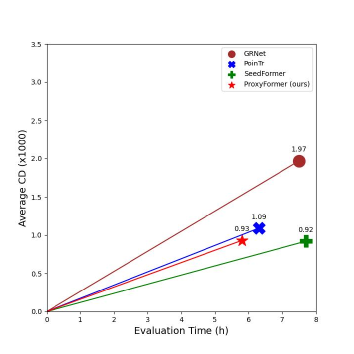
(a) CD vs. Eval. time on ShapeNet-55.

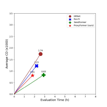
(b) CD vs. Eval. time on 34 seen categories.

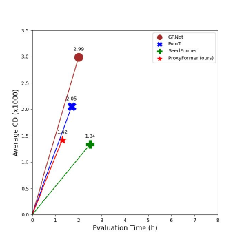
(c) CD vs. Eval. time on 21 novel categories.

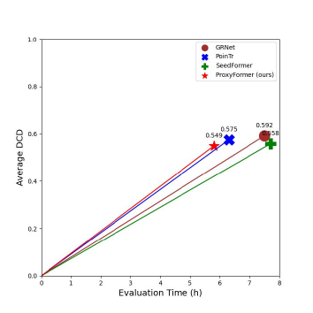
(d) DCD vs. Eval. time on ShapeNet-55.

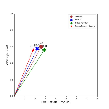
(e) DCD vs. Eval. time on 34 seen categories.

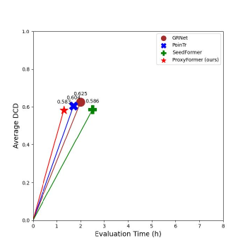
(f) DCD vs. Eval. time on 21 novel categories.

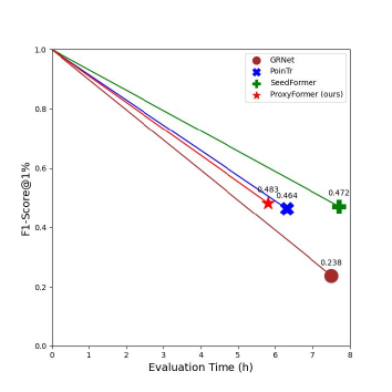
(g) F1 vs. Eval. time on ShapeNet-55.

(h) F1 vs. Eval. time on 34 seen categories.

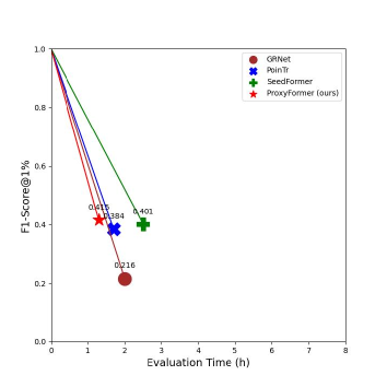
(i) F1 vs. Eval. time on 21 novel categories.

Figure 11: Performance comparison. The first column represents the comparison results on ShapeNet-55. The second column represents the comparison results on 34 seen categories in ShapeNet-34, and the third column represents the comparison results on 21 novel categories in ShapeNet-34. The first row represents Eval. time vs. CD. The second row represents Eval. time vs. DCD. The third row represents Eval. time vs. F1-Score@1%. In order to observe the distance between the values and the coordinates (0, 0) or (0, 1) more clearly, we connect them, so the lines in the figure have no practical meaning and are only used for comparison.

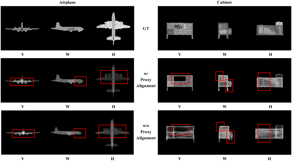
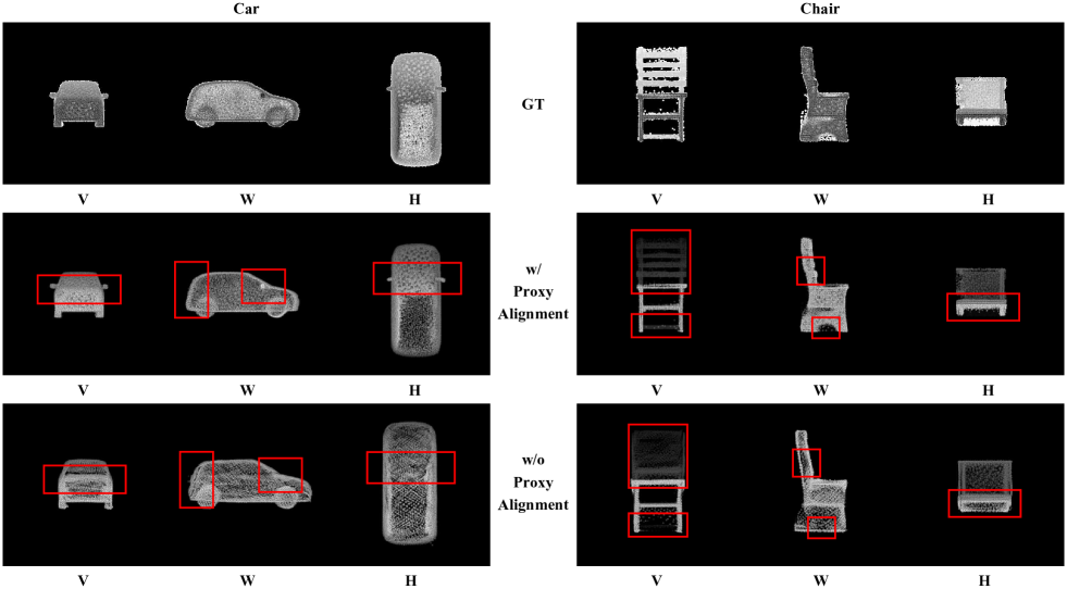
Figure 12: Three-view drawings of GT, results with proxy alignment and results without proxy alignment. Each figure represents vertical plane (V), width plane (W) and horizontal plane (H) from left to right. The result six categories of objects in the PCN are listed separately, and the red box indicates where Proxy Alignment contributes the most.

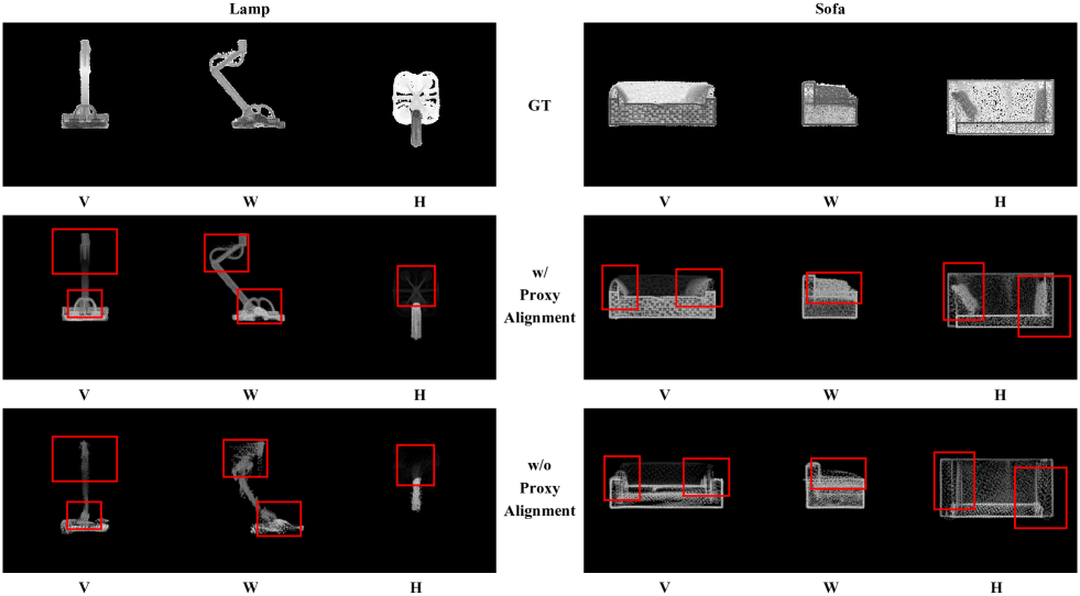
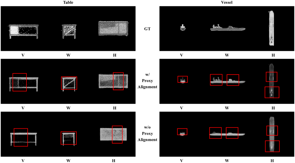
Figure 13: Three-view drawings of GT, results with proxy alignment and results without proxy alignment. Each figure represents vertical plane (V), width plane (W) and horizontal plane (H) from left to right. The result six categories of objects in the PCN are listed separately, and the red box indicates where Proxy Alignment contributes the most.

D.2 More experimental results

Three-views drawings. In Figs. 12 and 13, we have drawn three views of ProxyFormer on the PCN dataset, and we can see that proxy alignment plays a significant role in the point cloud completion task.

More qualitative results on PCN dataset. We show more visualization results of ProxyFormer on PCN dataset in Fig. 14. From this, we can find that our method is more sensitive to the concentrated distribution of missing part, which makes it impossible to easily distinguish the shape of objects from the existing point clouds, such as the second cabinet and the first car. But our method can complete its shape well, and the final result is basically consistent with GT.

More qualitative results on ShapeNet-55/34. In Figure 15, we show the visualization results of point cloud completion on ShapNet-55 by PoinTr [45], SeedFormer [52], and ProxyFormer. We can intuitively see that ProxyFormer can better complete the point cloud completion task. For example, for the table in the first row, although the resulting shape of PoinTr is complete, it fails to generate the details of the bottom of the table well, and SeedFormer introduces some noise points in the completion process, which affects the final result. But our method is able to take both shape and detail into account. Another example is the car in the fourth row. The point cloud contains not only a car, but also a person. There is a problem with the results of PoinTr and SeedFormer completion, that is, the distribution of point clouds is uneven, while ProxyFormer can better perceive the distribution of missing points, thereby generating a more reasonable complete point cloud. In Fig. 16, we also show more visualization results of ProxyFormer on the ShapNet-55. To better demonstrate the point cloud completion capability of our method, for each object, we show two different parts missing. For example, for the second bird house, we show both cases where the bottom and top are missing, and our method can easily get complete point clouds with local details.

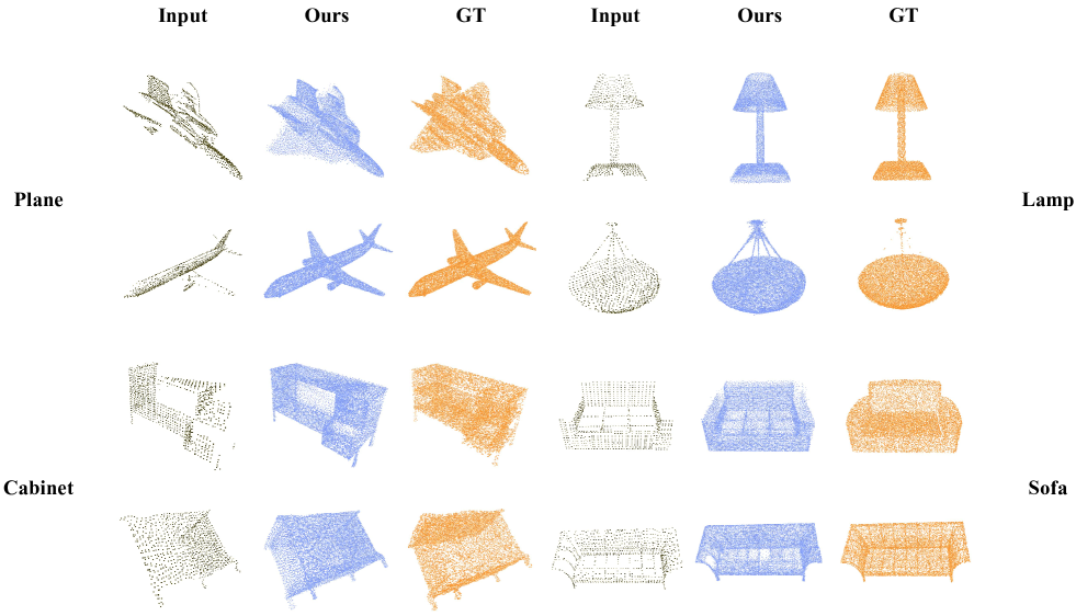
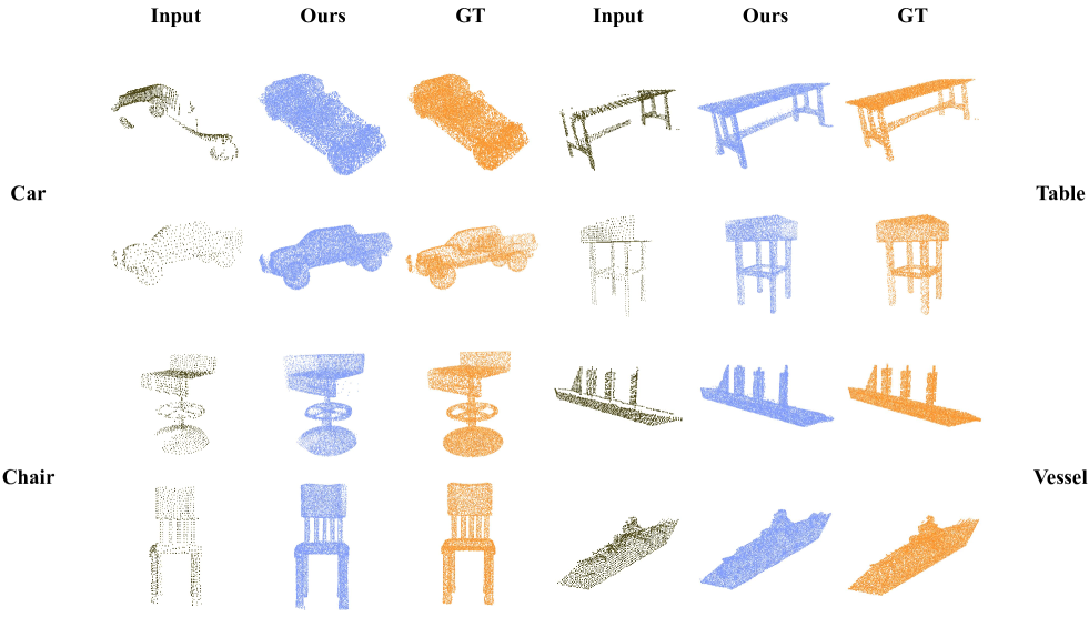
Figure 14: More visual completion results of ProxyFormer on PCN dataset. For each category in PCN, we show two results.

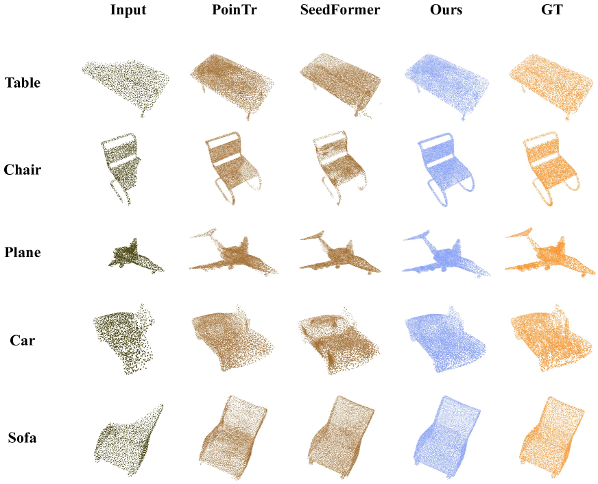
Figure 15: The visualization results of each method on ShapeNet-55, showing Table, Chair, Plane, Car and Sofa from top to bottom.

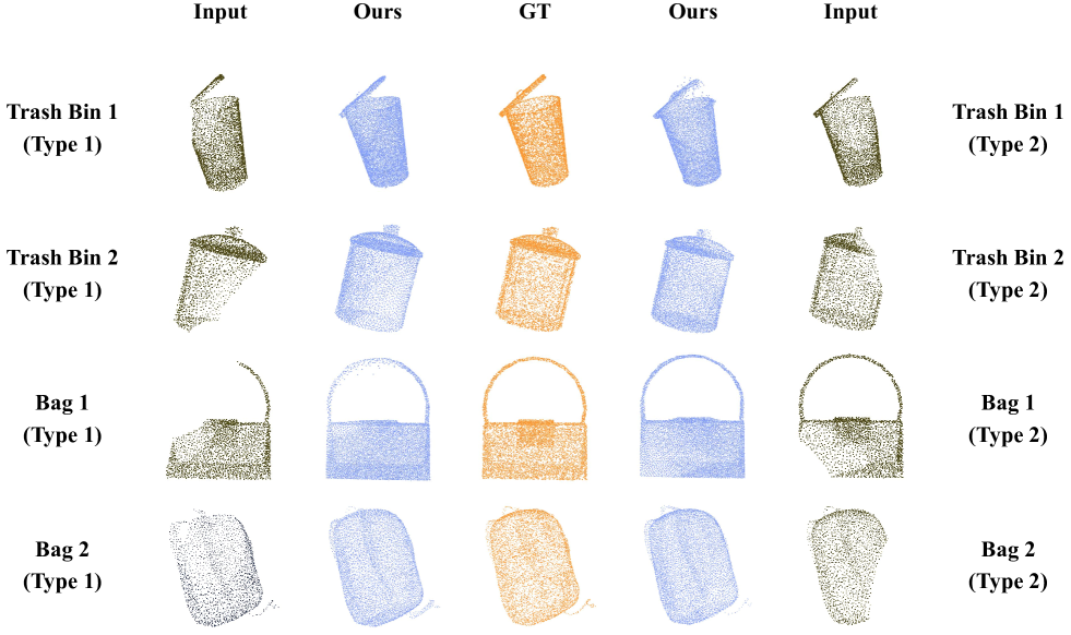
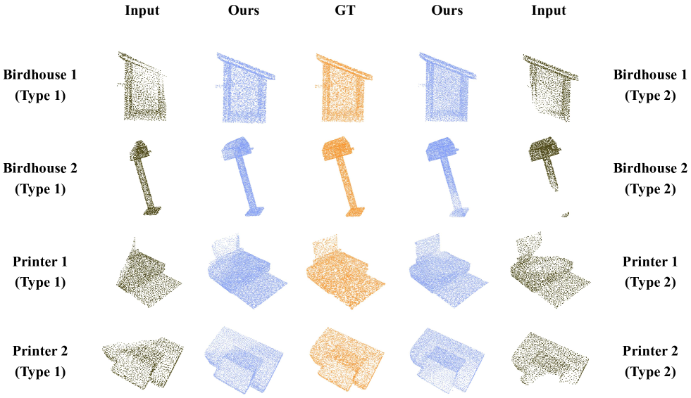
Figure 16: More visual completion results of ProxyFormer on ShapeNet-55. Each object contains two missing angles.

Detailed quantitative results on ShapeNet-55/34. We report complete results of our method on ShapeNet-55 in Tables 13 and 14 and results of novel categories on ShapeNet-34 in Tables 15 and 16. The models are tested under three difficulty levels: simple, moderate and hard. We can see that ProxyFormer achieves lowest DCD on almost all categories on the three settings.

Table 13: Detailed results on the ShapeNet-55 dataset, including Simple (S), Moderate (M) and Hard (H) three difficulties. For CD-$l_{2}$ ($\times 1000$), lower is better.

	GRNet			PoinTr			SeedFormer			Ours
	CD-S	CD-M	CD-H	CD-S	CD-M	CD-H	CD-S	CD-M	CD-H	CD-S	CD-M	CD-H
airplane	0.87	0.87	1.27	0.27	0.38	0.69	0.23	0.35	0.61	0.21	0.28	0.54
trash bin	1.69	2.01	3.48	0.80	1.15	2.15	0.73	1.08	1.94	0.70	1.04	1.98
bag	1.41	1.70	2.97	0.53	0.74	1.51	0.43	0.67	1.28	0.39	0.65	1.34
basket	1.65	1.84	3.15	0.73	0.88	1.82	0.65	0.83	1.54	0.64	0.74	1.40
bathtub	1.46	1.73	2.73	0.64	0.94	1.68	0.52	0.82	1.45	0.52	0.85	1.47
bed	1.64	2.03	3.70	0.76	1.10	2.26	0.63	0.91	1.89	0.62	0.91	2.04
bench	1.03	1.09	1.71	0.38	0.52	0.94	0.32	0.42	0.84	0.30	0.39	0.80
birdhouse	1.87	2.40	4.71	0.98	1.49	3.13	0.76	1.30	2.46	0.83	1.22	2.67
bookshelf	1.42	1.71	2.78	0.71	1.06	1.93	0.57	0.84	1.57	0.55	0.92	1.73
bottle	1.05	1.44	2.67	0.37	0.74	1.50	0.31	0.63	1.21	0.31	0.60	1.27
bowl	1.60	1.77	2.99	0.68	0.78	1.44	0.56	0.65	1.18	0.54	0.62	1.14
bus	1.06	1.16	1.48	0.42	0.55	0.79	0.42	0.55	0.73	0.40	0.46	0.59
cabinet	1.27	1.41	2.09	0.55	0.66	1.16	0.57	0.69	1.05	0.64	0.59	1.00
camera	2.14	3.15	6.09	1.10	2.03	4.34	0.83	1.68	3.45	0.82	1.77	4.04
can	1.58	2.11	3.81	0.68	1.19	2.14	0.58	1.03	1.79	0.55	1.02	1.86
cap	1.17	1.37	3.05	0.46	0.62	1.64	0.33	0.45	1.18	0.31	0.51	1.28
car	1.29	1.48	2.14	0.64	0.86	1.25	0.65	0.86	1.17	0.61	0.69	1.03
cellphone	0.82	0.91	1.18	0.32	0.39	0.60	0.31	0.40	0.54	0.26	0.38	0.45
chair	1.24	1.56	2.73	0.49	0.74	1.63	0.41	0.65	1.38	0.40	0.61	1.48
clock	1.46	1.66	2.67	0.62	0.84	1.65	0.53	0.74	1.35	0.50	0.67	1.45
keyboard	0.74	0.81	1.09	0.30	0.39	0.45	0.28	0.36	0.45	0.27	0.33	0.43
dishwasher	1.43	1.59	2.53	0.55	0.69	1.42	0.56	0.69	1.30	0.57	0.61	1.21
display	1.13	1.38	2.29	0.48	0.67	1.33	0.39	0.59	1.10	0.46	0.62	1.18
earphone	1.78	2.18	5.33	0.81	1.38	3.78	0.64	1.04	2.75	0.62	1.12	3.36
faucet	1.81	2.32	4.91	0.71	1.42	3.49	0.55	1.15	2.63	0.49	1.16	3.01
filecabinet	1.46	1.71	2.89	0.63	0.84	1.69	0.63	0.84	1.49	0.74	0.79	1.45
guitar	0.44	0.48	0.76	0.14	0.21	0.42	0.13	0.19	0.32	0.14	0.20	0.28
helmet	2.33	3.18	6.03	0.99	1.93	4.22	0.79	1.52	3.61	0.76	1.60	3.91
jar	1.72	2.37	4.37	0.77	1.33	2.87	0.63	1.13	2.36	0.62	1.13	2.69
knife	0.72	0.66	0.96	0.20	0.33	0.56	0.15	0.28	0.45	0.15	0.21	0.43
lamp	1.68	2.43	5.17	0.64	1.40	3.58	0.45	1.06	2.67	0.42	1.05	3.03
laptop	0.83	0.87	1.28	0.32	0.34	0.60	0.32	0.37	0.55	0.30	0.31	0.42
loudspeaker	1.75	2.08	3.45	0.78	1.16	2.17	0.67	1.01	1.80	0.66	1.03	1.89
mailbox	1.15	1.59	3.42	0.39	0.78	2.56	0.30	0.67	2.04	0.30	0.65	2.17
microphone	2.09	2.76	5.70	0.70	1.66	4.48	0.62	1.61	3.66	0.59	1.58	3.98
microwaves	1.51	1.72	2.76	0.67	0.83	1.82	0.63	0.79	1.47	0.61	0.69	1.35
motorbike	1.38	1.52	2.26	0.75	1.10	1.92	0.68	0.96	1.44	0.67	0.96	1.49
mug	1.75	2.16	3.79	0.91	1.17	2.35	0.79	1.03	2.06	0.75	0.92	2.00
piano	1.53	1.82	3.21	0.76	1.06	2.23	0.62	0.87	1.79	0.55	0.85	1.73
pillow	1.42	1.67	3.04	0.61	0.82	1.56	0.48	0.75	1.41	0.49	0.71	1.35
pistol	1.11	1.06	1.76	0.43	0.66	1.30	0.37	0.56	0.96	0.34	0.52	0.90
flowerpot	2.02	2.48	4.19	1.01	1.51	2.77	0.93	1.30	2.32	0.89	1.39	2.52
printer	1.56	2.38	4.24	0.73	1.21	2.47	0.58	1.11	2.13	0.53	1.09	2.08
remote	0.89	1.05	1.29	0.36	0.53	0.71	0.29	0.46	0.62	0.20	0.33	0.54
rifle	0.83	0.77	1.16	0.30	0.45	0.79	0.27	0.41	0.66	0.21	0.32	0.50
rocket	0.78	0.92	1.44	0.23	0.48	0.99	0.21	0.46	0.83	0.21	0.38	0.80
skateboard	0.82	0.87	1.24	0.28	0.38	0.62	0.23	0.32	0.62	0.19	0.28	0.56
sofa	1.35	1.45	2.32	0.56	0.67	1.14	0.50	0.62	1.02	0.49	0.57	1.01
stove	1.46	1.72	3.22	0.63	0.92	1.73	0.59	0.87	1.49	0.68	0.88	1.67
table	1.15	1.33	2.33	0.46	0.64	1.31	0.41	0.58	1.18	0.39	0.48	1.06
telephone	0.81	0.89	1.18	0.31	0.38	0.59	0.31	0.39	0.55	0.28	0.32	0.48
tower	1.26	1.69	3.06	0.55	0.90	1.95	0.47	0.84	1.65	0.46	0.82	1.67
train	1.09	1.14	1.61	0.50	0.70	1.12	0.51	0.66	1.01	0.49	0.61	0.97
watercraft	1.09	1.12	1.65	0.41	0.62	1.07	0.35	0.56	0.92	0.44	0.62	1.04
washer	1.72	2.05	4.19	0.75	1.06	2.44	0.64	0.91	2.04	0.63	0.94	2.26
mean	1.35	1.63	2.86	0.58	0.88	1.80	0.50	0.77	1.49	0.49	0.75	1.55

Table 14: Detailed results on the ShapeNet-55 dataset, including Simple (S), Moderate (M) and Hard (H) three difficulties, For DCD, lower is better.

	GRNet			PoinTr			SeedFormer			Ours
	DCD-S	DCD-M	DCD-H	DCD-S	DCD-M	DCD-H	DCD-S	DCD-M	DCD-H	DCD-S	DCD-M	DCD-H
airplane	0.520	0.559	0.614	0.487	0.524	0.608	0.478	0.505	0.574	0.475	0.496	0.565
trash bin	0.586	0.616	0.705	0.557	0.599	0.679	0.547	0.588	0.648	0.544	0.578	0.653
bag	0.518	0.563	0.653	0.510	0.549	0.628	0.503	0.546	0.590	0.483	0.515	0.588
basket	0.559	0.593	0.648	0.533	0.573	0.630	0.530	0.558	0.609	0.522	0.548	0.616
bathtub	0.503	0.553	0.646	0.499	0.544	0.619	0.498	0.523	0.609	0.492	0.519	0.589
bed	0.553	0.620	0.694	0.544	0.589	0.661	0.537	0.583	0.637	0.528	0.554	0.622
bench	0.528	0.546	0.607	0.507	0.531	0.589	0.506	0.504	0.543	0.483	0.494	0.539
birdhouse	0.576	0.617	0.722	0.562	0.597	0.697	0.554	0.585	0.650	0.538	0.579	0.658
bookshelf	0.563	0.589	0.678	0.541	0.569	0.655	0.523	0.562	0.623	0.519	0.554	0.631
bottle	0.505	0.546	0.635	0.485	0.533	0.628	0.458	0.516	0.606	0.455	0.508	0.605
bowl	0.545	0.591	0.676	0.531	0.560	0.641	0.524	0.529	0.613	0.507	0.529	0.602
bus	0.533	0.559	0.606	0.525	0.547	0.599	0.521	0.525	0.584	0.499	0.523	0.570
cabinet	0.590	0.593	0.643	0.557	0.577	0.626	0.532	0.548	0.595	0.521	0.544	0.596
camera	0.583	0.647	0.728	0.558	0.615	0.701	0.547	0.608	0.670	0.535	0.584	0.671
can	0.549	0.599	0.651	0.527	0.571	0.649	0.511	0.550	0.621	0.500	0.542	0.616
cap	0.528	0.544	0.640	0.495	0.541	0.638	0.491	0.539	0.609	0.474	0.510	0.612
car	0.614	0.660	0.683	0.581	0.631	0.673	0.566	0.607	0.661	0.565	0.592	0.644
cellphone	0.508	0.509	0.568	0.483	0.506	0.541	0.482	0.497	0.520	0.458	0.480	0.521
chair	0.526	0.559	0.623	0.505	0.555	0.620	0.501	0.527	0.609	0.488	0.523	0.606
clock	0.543	0.578	0.657	0.528	0.561	0.634	0.515	0.554	0.594	0.502	0.531	0.595
keyboard	0.515	0.528	0.553	0.499	0.511	0.541	0.477	0.498	0.510	0.473	0.483	0.515
dishwasher	0.566	0.600	0.643	0.540	0.568	0.629	0.514	0.536	0.593	0.508	0.535	0.596
display	0.532	0.544	0.595	0.517	0.544	0.587	0.483	0.519	0.554	0.483	0.508	0.560
earphone	0.579	0.609	0.708	0.555	0.605	0.694	0.539	0.603	0.669	0.529	0.571	0.675
faucet	0.512	0.602	0.681	0.502	0.573	0.687	0.495	0.565	0.663	0.483	0.548	0.665
filecabinet	0.580	0.615	0.662	0.559	0.579	0.644	0.529	0.562	0.619	0.529	0.556	0.616
guitar	0.499	0.538	0.616	0.488	0.514	0.602	0.459	0.495	0.571	0.456	0.493	0.578
helmet	0.591	0.613	0.699	0.567	0.608	0.695	0.551	0.597	0.668	0.538	0.586	0.676
jar	0.574	0.598	0.679	0.541	0.590	0.669	0.516	0.567	0.650	0.512	0.565	0.660
knife	0.486	0.571	0.651	0.470	0.544	0.643	0.464	0.533	0.606	0.461	0.518	0.613
lamp	0.526	0.587	0.717	0.520	0.581	0.689	0.510	0.578	0.677	0.488	0.553	0.657
laptop	0.501	0.538	0.558	0.492	0.510	0.557	0.488	0.506	0.548	0.473	0.488	0.532
loudspeaker	0.561	0.589	0.669	0.548	0.583	0.649	0.544	0.566	0.622	0.526	0.556	0.620
mailbox	0.499	0.543	0.674	0.477	0.540	0.667	0.465	0.520	0.620	0.458	0.518	0.628
microphone	0.546	0.622	0.709	0.511	0.587	0.701	0.503	0.579	0.681	0.490	0.560	0.674
microwaves	0.559	0.580	0.634	0.546	0.566	0.621	0.541	0.544	0.614	0.522	0.544	0.597
motorbike	0.653	0.690	0.714	0.623	0.657	0.709	0.614	0.652	0.687	0.596	0.627	0.695
mug	0.582	0.618	0.706	0.560	0.588	0.678	0.536	0.585	0.657	0.535	0.569	0.644
piano	0.550	0.585	0.658	0.538	0.573	0.632	0.537	0.552	0.611	0.519	0.544	0.602
pillow	0.495	0.529	0.665	0.494	0.529	0.633	0.485	0.518	0.613	0.474	0.510	0.595
pistol	0.557	0.586	0.668	0.529	0.571	0.655	0.509	0.570	0.620	0.506	0.545	0.627
flowerpot	0.608	0.626	0.701	0.596	0.622	0.697	0.591	0.609	0.667	0.570	0.601	0.671
printer	0.560	0.595	0.648	0.543	0.578	0.640	0.529	0.561	0.619	0.513	0.544	0.617
remote	0.510	0.538	0.564	0.479	0.506	0.559	0.468	0.483	0.538	0.454	0.483	0.536
rifle	0.534	0.572	0.626	0.519	0.562	0.646	0.500	0.551	0.632	0.497	0.539	0.616
rocket	0.512	0.567	0.670	0.511	0.553	0.650	0.503	0.546	0.610	0.484	0.524	0.616
skateboard	0.517	0.525	0.586	0.484	0.507	0.589	0.461	0.503	0.580	0.461	0.483	0.566
sofa	0.554	0.588	0.603	0.532	0.559	0.596	0.525	0.541	0.563	0.507	0.523	0.567
stove	0.562	0.577	0.650	0.528	0.554	0.634	0.521	0.550	0.601	0.516	0.546	0.606
table	0.513	0.529	0.588	0.499	0.529	0.579	0.491	0.517	0.576	0.481	0.502	0.553
telephone	0.506	0.532	0.564	0.483	0.498	0.554	0.467	0.495	0.529	0.457	0.476	0.516
tower	0.571	0.622	0.676	0.536	0.593	0.684	0.513	0.567	0.659	0.512	0.562	0.649
train	0.530	0.589	0.660	0.529	0.565	0.629	0.520	0.563	0.618	0.518	0.541	0.599
watercraft	0.525	0.551	0.652	0.507	0.547	0.641	0.496	0.524	0.605	0.488	0.524	0.599
washer	0.553	0.591	0.649	0.540	0.570	0.647	0.533	0.567	0.621	0.522	0.551	0.612
mean	0.545	0.581	0.650	0.525	0.562	0.637	0.513	0.549	0.612	0.502	0.536	0.608

Table 15: Detailed results on the 21 unseen categories of ShapeNet-34 dataset, including Simple (S), Moderate (M) and Hard (H) three difficulties. For CD-$l_{2}$ ($\times 1000$), lower is better.

	GRNet			PoinTr			SeedFormer			Ours
	CD-S	CD-M	CD-H	CD-S	CD-M	CD-H	CD-S	CD-M	CD-H	CD-S	CD-M	CD-H
bag	1.47	1.88	3.45	0.96	1.34	2.08	0.49	0.82	1.45	0.48	0.80	1.43
basket	1.78	1.94	4.18	1.04	1.40	2.90	0.60	0.85	1.98	0.57	0.91	2.08
birdhouse	1.89	2.34	5.16	1.22	1.79	3.45	0.72	1.19	2.31	0.51	1.03	2.00
bowl	1.77	1.97	3.90	1.05	1.32	2.40	0.60	0.77	1.50	0.63	0.96	1.79
camera	2.31	3.38	7.20	1.63	2.67	4.97	0.89	1.77	3.75	0.88	1.94	4.04
can	1.53	1.80	3.08	0.80	1.17	2.85	0.56	0.89	1.57	0.50	0.64	1.73
cap	3.29	4.87	13.02	1.40	2.74	8.35	0.50	1.34	5.19	0.51	1.57	6.38
keyboard	0.73	0.77	1.11	0.43	0.45	0.63	0.32	0.41	0.60	0.29	0.34	0.59
dishwasher	1.79	1.70	3.27	0.93	1.05	2.04	0.63	0.78	1.44	0.72	0.90	1.49
earphone	4.29	4.16	10.30	2.03	5.10	10.69	1.18	2.78	6.71	1.09	2.96	8.98
helmet	3.06	4.38	10.27	1.86	3.30	6.96	1.10	2.27	4.78	1.32	2.44	5.74
mailbox	1.52	1.90	4.33	1.03	1.47	3.34	0.56	0.99	2.06	0.74	1.09	2.14
microphone	2.29	3.23	8.41	1.25	2.27	5.47	0.80	1.61	4.21	0.73	1.73	3.70
microwaves	1.74	1.81	3.82	1.01	1.18	2.14	0.64	0.83	1.69	0.60	0.90	1.58
pillow	1.43	1.69	3.43	0.92	1.24	2.39	0.43	0.66	1.45	0.43	0.73	1.07
printer	1.82	2.41	5.09	1.18	1.76	3.10	0.69	1.25	2.33	0.59	1.40	2.56
remote	0.82	1.02	1.29	0.44	0.58	0.78	0.27	0.42	0.61	0.29	0.51	0.67
rocket	0.97	0.79	1.60	0.39	0.72	1.39	0.28	0.51	1.02	0.26	0.46	0.82
skateboard	0.93	1.07	1.83	0.52	0.80	1.31	0.35	0.56	0.92	0.35	0.61	0.78
tower	1.35	1.80	3.85	0.82	1.35	2.48	0.51	0.92	1.87	0.59	0.83	1.79
washer	1.83	1.97	5.28	1.04	1.39	2.73	0.61	0.87	1.94	0.62	0.89	1.90
mean	1.84	2.23	4.95	1.05	1.67	3.45	0.61	1.07	2.35	0.60	1.13	2.54

Table 16: Detailed results on the 21 unseen categories of ShapeNet-34 dataset, including Simple (S), Moderate (M) and Hard (H) three difficulties. For DCD, lower is better.

	GRNet			PoinTr			SeedFormer			Ours
	DCD-S	DCD-M	DCD-H	DCD-S	DCD-M	DCD-H	DCD-S	DCD-M	DCD-H	DCD-S	DCD-M	DCD-H
bag	0.521	0.597	0.617	0.506	0.573	0.593	0.489	0.556	0.572	0.492	0.556	0.573
basket	0.599	0.631	0.633	0.574	0.621	0.626	0.555	0.605	0.613	0.548	0.608	0.614
birdhouse	0.610	0.678	0.708	0.580	0.658	0.680	0.561	0.632	0.659	0.554	0.615	0.641
bowl	0.603	0.637	0.659	0.581	0.624	0.631	0.558	0.595	0.614	0.553	0.597	0.616
camera	0.624	0.640	0.708	0.594	0.629	0.689	0.574	0.618	0.666	0.587	0.619	0.665
can	0.570	0.628	0.637	0.550	0.617	0.582	0.525	0.587	0.568	0.518	0.571	0.569
cap	0.632	0.737	0.783	0.598	0.715	0.757	0.568	0.689	0.743	0.560	0.692	0.742
keyboard	0.484	0.513	0.535	0.461	0.501	0.519	0.450	0.484	0.505	0.446	0.477	0.493
dishwasher	0.597	0.631	0.701	0.564	0.609	0.681	0.554	0.590	0.658	0.566	0.591	0.656
earphone	0.695	0.687	0.803	0.666	0.671	0.773	0.655	0.645	0.739	0.660	0.648	0.751
helmet	0.669	0.730	0.781	0.639	0.717	0.761	0.627	0.706	0.738	0.632	0.699	0.738
mailbox	0.563	0.571	0.627	0.547	0.552	0.605	0.526	0.536	0.582	0.518	0.541	0.581
microphone	0.618	0.717	0.764	0.585	0.700	0.746	0.573	0.672	0.732	0.566	0.666	0.734
microwaves	0.609	0.622	0.660	0.575	0.604	0.634	0.557	0.582	0.623	0.549	0.584	0.622
pillow	0.595	0.620	0.626	0.575	0.606	0.603	0.562	0.577	0.578	0.556	0.578	0.568
printer	0.631	0.675	0.725	0.607	0.665	0.700	0.593	0.650	0.687	0.588	0.651	0.683
remote	0.496	0.516	0.542	0.480	0.494	0.526	0.462	0.480	0.508	0.456	0.470	0.507
rocket	0.499	0.510	0.560	0.476	0.501	0.542	0.457	0.488	0.518	0.449	0.469	0.516
skateboard	0.493	0.539	0.607	0.474	0.527	0.580	0.463	0.511	0.567	0.456	0.514	0.566
tower	0.545	0.602	0.685	0.526	0.590	0.667	0.500	0.563	0.655	0.494	0.544	0.656
washer	0.586	0.612	0.717	0.562	0.591	0.698	0.551	0.566	0.686	0.544	0.569	0.686
mean	0.583	0.623	0.670	0.558	0.608	0.647	0.541	0.587	0.629	0.538	0.584	0.627

References

- [1] Panos Achlioptas, Olga Diamanti, Ioannis Mitliagkas, and Leonidas Guibas. Learning representations and generative models for 3d point clouds. In International conference on machine learning, pages 40–49. PMLR, 2018.
- [2] Angel X Chang, Thomas Funkhouser, Leonidas Guibas, Pat Hanrahan, Qixing Huang, Zimo Li, Silvio Savarese, Manolis Savva, Shuran Song, Hao Su, et al. Shapenet: An information-rich 3d model repository. arXiv preprint arXiv:1512.03012, 2015.
- [3] Honghua Chen, Zeyong Wei, Yabin Xu, Mingqiang Wei, and Jun Wang. Imlovenet: Misaligned image-supported registration network for low-overlap point cloud pairs. In ACM SIGGRAPH 2022 Conference Proceedings, pages 1–9, 2022.
- [4] Jun-Kun Chen and Yu-Xiong Wang. Pointtree: Transformation-robust point cloud encoder with relaxed kd trees. arXiv preprint arXiv:2208.05962, 2022.
- [5] Yi-Nan Chen, Hang Dai, and Yong Ding. Pseudo-stereo for monocular 3d object detection in autonomous driving. In Proceedings of the IEEE/CVF Conference on Computer Vision and Pattern Recognition, pages 887–897, 2022.
- [6] Haoqiang Fan, Hao Su, and Leonidas J Guibas. A point set generation network for 3d object reconstruction from a single image. In Proceedings of the IEEE conference on computer vision and pattern recognition, pages 605–613, 2017.
- [7] Andreas Geiger, Philip Lenz, Christoph Stiller, and Raquel Urtasun. Vision meets robotics: The kitti dataset. The International Journal of Robotics Research, 32(11):1231–1237, 2013.
- [8] Thibault Groueix, Matthew Fisher, Vladimir G Kim, Bryan C Russell, and Mathieu Aubry. A papier-mâché approach to learning 3d surface generation. In Proceedings of the IEEE conference on computer vision and pattern recognition, pages 216–224, 2018.
- [9] Meng-Hao Guo, Jun-Xiong Cai, Zheng-Ning Liu, Tai-Jiang Mu, Ralph R Martin, and Shi-Min Hu. Pct: Point cloud transformer. Computational Visual Media, 7(2):187–199, 2021.
- [10] Zhixing Hou, Yan Yan, Chengzhong Xu, and Hui Kong. Hitpr: Hierarchical transformer for place recognition in point cloud. arXiv preprint arXiv:2204.05481, 2022.
- [11] Zitian Huang, Yikuan Yu, Jiawen Xu, Feng Ni, and Xinyi Le. Pf-net: Point fractal network for 3d point cloud completion. In Proceedings of the IEEE/CVF conference on computer vision and pattern recognition, pages 7662–7670, 2020.
- [12] Stephen James, Kentaro Wada, Tristan Laidlow, and Andrew J Davison. Coarse-to-fine q-attention: Efficient learning for visual robotic manipulation via discretisation. In Proceedings of the IEEE/CVF Conference on Computer Vision and Pattern Recognition, pages 13739–13748, 2022.
- [13] Vladimir G Kim, Wilmot Li, Niloy J Mitra, Siddhartha Chaudhuri, Stephen DiVerdi, and Thomas Funkhouser. Learning part-based templates from large collections of 3d shapes. ACM Transactions on Graphics (TOG), 32(4):1–12, 2013.
- [14] Peizhao Li, Pu Wang, Karl Berntorp, and Hongfu Liu. Exploiting temporal relations on radar perception for autonomous driving. In Proceedings of the IEEE/CVF Conference on Computer Vision and Pattern Recognition, pages 17071–17080, 2022.
- [15] Yangyan Li, Angela Dai, Leonidas Guibas, and Matthias Nießner. Database-assisted object retrieval for real-time 3d reconstruction. In Computer graphics forum, volume 34, pages 435–446. Wiley Online Library, 2015.
- [16] Jianjie Lin, Markus Rickert, Alexander Perzylo, and Alois Knoll. Pctma-net: Point cloud transformer with morphing atlas-based point generation network for dense point cloud completion. In 2021 IEEE/RSJ International Conference on Intelligent Robots and Systems (IROS), pages 5657–5663. IEEE, 2021.
- [17] Kunliang Liu, Ouk Choi, Jianming Wang, and Wonjun Hwang. Cdgnet: Class distribution guided network for human parsing. In Proceedings of the IEEE/CVF Conference on Computer Vision and Pattern Recognition, pages 4473–4482, 2022.
- [18] Minghua Liu, Lu Sheng, Sheng Yang, Jing Shao, and Shi-Min Hu. Morphing and sampling network for dense point cloud completion. In Proceedings of the AAAI conference on artificial intelligence, volume 34, pages 11596–11603, 2020.
- [19] Zhijian Liu, Haotian Tang, Shengyu Zhao, Kevin Shao, and Song Han. Pvnas: 3d neural architecture search with point-voxel convolution. arXiv preprint arXiv:2204.11797, 2022.
- [20] Ilya Loshchilov and Frank Hutter. Fixing weight decay regularization in adam. 2018.
- [21] Niloy J Mitra, Mark Pauly, Michael Wand, and Duygu Ceylan. Symmetry in 3d geometry: Extraction and applications. In Computer Graphics Forum, volume 32, pages 1–23. Wiley Online Library, 2013.
- [22] Liangliang Nan, Ke Xie, and Andrei Sharf. A search-classify approach for cluttered indoor scene understanding. ACM Transactions on Graphics (TOG), 31(6):1–10, 2012.
- [23] Adam Paszke, Sam Gross, Francisco Massa, Adam Lerer, James Bradbury, Gregory Chanan, Trevor Killeen, Zeming Lin, Natalia Gimelshein, Luca Antiga, et al. Pytorch: An imperative style, high-performance deep learning library. Advances in neural information processing systems, 32, 2019.
- [24] Mark Pauly, Niloy J Mitra, Johannes Wallner, Helmut Pottmann, and Leonidas J Guibas. Discovering structural regularity in 3d geometry. In ACM SIGGRAPH 2008 papers, pages 1–11. 2008.
- [25] Charles R Qi, Hao Su, Kaichun Mo, and Leonidas J Guibas. Pointnet: Deep learning on point sets for 3d classification and segmentation. In Proceedings of the IEEE conference on computer vision and pattern recognition, pages 652–660, 2017.
- [26] Charles Ruizhongtai Qi, Li Yi, Hao Su, and Leonidas J Guibas. Pointnet++: Deep hierarchical feature learning on point sets in a metric space. Advances in neural information processing systems, 30, 2017.
- [27] Lyne P Tchapmi, Vineet Kosaraju, Hamid Rezatofighi, Ian Reid, and Silvio Savarese. Topnet: Structural point cloud decoder. In Proceedings of the IEEE/CVF Conference on Computer Vision and Pattern Recognition, pages 383–392, 2019.
- [28] Dong Tian, Hideaki Ochimizu, Chen Feng, Robert Cohen, and Anthony Vetro. Geometric distortion metrics for point cloud compression. In 2017 IEEE International Conference on Image Processing (ICIP), pages 3460–3464. IEEE, 2017.
- [29] Federico Tombari, Samuele Salti, and Luigi Di Stefano. Unique signatures of histograms for local surface description. In European conference on computer vision, pages 356–369. Springer, 2010.
- [30] Kutub Uddin, Tae Hyun Jeong, and Byung Tae Oh. Incomplete region estimation and restoration of 3d point cloud human face datasets. Sensors, 22(3):723, 2022.
- [31] Ashish Vaswani, Noam Shazeer, Niki Parmar, Jakob Uszkoreit, Llion Jones, Aidan N Gomez, Łukasz Kaiser, and Illia Polosukhin. Attention is all you need. Advances in neural information processing systems, 30, 2017.
- [32] Xiaogang Wang, Marcelo H Ang Jr, and Gim Hee Lee. Cascaded refinement network for point cloud completion. In Proceedings of the IEEE/CVF Conference on Computer Vision and Pattern Recognition, pages 790–799, 2020.
- [33] Yue Wang, Yongbin Sun, Ziwei Liu, Sanjay E Sarma, Michael M Bronstein, and Justin M Solomon. Dynamic graph cnn for learning on point clouds. Acm Transactions On Graphics (tog), 38(5):1–12, 2019.
- [34] Xin Wen, Peng Xiang, Zhizhong Han, Yan-Pei Cao, Pengfei Wan, Wen Zheng, and Yu-Shen Liu. Pmp-net: Point cloud completion by learning multi-step point moving paths. In Proceedings of the IEEE/CVF Conference on Computer Vision and Pattern Recognition, pages 7443–7452, 2021.
- [35] Xin Wen, Peng Xiang, Zhizhong Han, Yan-Pei Cao, Pengfei Wan, Wen Zheng, and Yu-Shen Liu. Pmp-net++: Point cloud completion by transformer-enhanced multi-step point moving paths. IEEE Transactions on Pattern Analysis and Machine Intelligence, 2022.
- [36] Hang Wu and Yubin Miao. Lra-net: local region attention network for 3d point cloud completion. In Thirteenth International Conference on Machine Vision, volume 11605, pages 357–367. SPIE, 2021.
- [37] Hang Wu, Yubin Miao, and Ruochong Fu. Point cloud completion using multiscale feature fusion and cross-regional attention. Image and Vision Computing, 111:104193, 2021.
- [38] Rundi Wu, Xuelin Chen, Yixin Zhuang, and Baoquan Chen. Multimodal shape completion via conditional generative adversarial networks. In European Conference on Computer Vision, pages 281–296. Springer, 2020.
- [39] Tong Wu, Liang Pan, Junzhe Zhang, Tai Wang, Ziwei Liu, and Dahua Lin. Density-aware chamfer distance as a comprehensive metric for point cloud completion. arXiv preprint arXiv:2111.12702, 2021.
- [40] Yaqi Xia, Yan Xia, Wei Li, Rui Song, Kailang Cao, and Uwe Stilla. Asfm-net: Asymmetrical siamese feature matching network for point completion. In Proceedings of the 29th ACM International Conference on Multimedia, pages 1938–1947, 2021.
- [41] Peng Xiang, Xin Wen, Yu-Shen Liu, Yan-Pei Cao, Pengfei Wan, Wen Zheng, and Zhizhong Han. Snowflakenet: Point cloud completion by snowflake point deconvolution with skip-transformer. In Proceedings of the IEEE/CVF international conference on computer vision, pages 5499–5509, 2021.
- [42] Haozhe Xie, Hongxun Yao, Shangchen Zhou, Jiageng Mao, Shengping Zhang, and Wenxiu Sun. Grnet: Gridding residual network for dense point cloud completion. In European Conference on Computer Vision, pages 365–381. Springer, 2020.
- [43] Zelin Xu, Yichen Zhang, Ke Chen, and Kui Jia. Bico-net: Regress globally, match locally for robust 6d pose estimation. arXiv preprint arXiv:2205.03536, 2022.
- [44] Yaoqing Yang, Chen Feng, Yiru Shen, and Dong Tian. Foldingnet: Point cloud auto-encoder via deep grid deformation. In Proceedings of the IEEE conference on computer vision and pattern recognition, pages 206–215, 2018.
- [45] Xumin Yu, Yongming Rao, Ziyi Wang, Zuyan Liu, Jiwen Lu, and Jie Zhou. Pointr: Diverse point cloud completion with geometry-aware transformers. In Proceedings of the IEEE/CVF international conference on computer vision, pages 12498–12507, 2021.
- [46] Wentao Yuan, Tejas Khot, David Held, Christoph Mertz, and Martial Hebert. Pcn: Point completion network. In 2018 International Conference on 3D Vision (3DV), pages 728–737. IEEE, 2018.
- [47] Qingzhao Zhang, Shengtuo Hu, Jiachen Sun, Qi Alfred Chen, and Z Morley Mao. On adversarial robustness of trajectory prediction for autonomous vehicles. In Proceedings of the IEEE/CVF Conference on Computer Vision and Pattern Recognition, pages 15159–15168, 2022.
- [48] Wenxiao Zhang, Qingan Yan, and Chunxia Xiao. Detail preserved point cloud completion via separated feature aggregation. In European Conference on Computer Vision, pages 512–528. Springer, 2020.
- [49] Hengshuang Zhao, Li Jiang, Chi-Wing Fu, and Jiaya Jia. Pointweb: Enhancing local neighborhood features for point cloud processing. In Proceedings of the IEEE/CVF conference on computer vision and pattern recognition, pages 5565–5573, 2019.
- [50] Hengshuang Zhao, Li Jiang, Jiaya Jia, Philip HS Torr, and Vladlen Koltun. Point transformer. In Proceedings of the IEEE/CVF International Conference on Computer Vision, pages 16259–16268, 2021.
- [51] Wei Zhao, Shuming Gao, and Hongwei Lin. A robust hole-filling algorithm for triangular mesh. The Visual Computer, 23(12):987–997, 2007.
- [52] Haoran Zhou, Yun Cao, Wenqing Chu, Junwei Zhu, Tong Lu, Ying Tai, and Chengjie Wang. Seedformer: Patch seeds based point cloud completion with upsample transformer. arXiv preprint arXiv:2207.10315, 2022.
- [53] Yin Zhou and Oncel Tuzel. Voxelnet: End-to-end learning for point cloud based 3d object detection. In Proceedings of the IEEE conference on computer vision and pattern recognition, pages 4490–4499, 2018.
- [54] Liping Zhu, Bingyao Wang, Gangyi Tian, Wenjie Wang, and Chengyang Li. Towards point cloud completion: Point rank sampling and cross-cascade graph cnn. Neurocomputing, 461:1–16, 2021.