Federated Covariate Shift Adaptation for Missing Target Output Values

Abstract

The most recent multi-source covariate shift algorithm is an efficient hyperparameter optimization algorithm for missing target output. In this paper, we extend this algorithm to the framework of federated learning. For data islands in federated learning and covariate shift adaptation, we propose the federated domain adaptation estimate of the target risk which is asymptotically unbiased with a desirable asymptotic variance property. We construct a weighted model for the target task and propose the federated covariate shift adaptation algorithm which works preferably in our setting. The efficacy of our method is justified both theoretically and empirically.

(Day Month Year)

AMS Subject Classification: 62J07, 62-08

1 Introduction

Covariate shift adaptation has been a pivotal part of transfer learning.[25] It is a prevalent setting for machine learning in which the feature distributions differ between the train (source) and test (target) domains, while the conditional distributions of the output variable given the feature variable remain unchanged, see Ref. 2000Improving. In this setting, when the output values of the target data are missing, the multi-source covariate shift (MS-CS)[17] algorithm can use multiple relevant source datasets whose output values are available to predict the target task.

One critical, but often overlooked assumption in MS-CS is that we can merge data from all sources as a training set. However, this assumption is not satisfied in many cases. For example, we need to predict the disease scores for patients in a new (target) hospital, but we only have historical medical outcome data from some source hospitals other than the target one. Furthermore, to protect patient privacy, each source hospital does not allow its data to leave its local area or to be disclosed, resulting in data islands. In this case, the MS-CS algorithm is infeasible. Fortunately, this issue can be well-solved in federated learning since it provides a privacy protection mechanism and allows us to learn and save locally at each node rather than share data or parameters, see Ref. 2018Aby,2017Practical,2017SecureML and 2019Federated.

In this paper, we extend the MS-CS algorithm to the federated learning framework. The difficulty in conducting MS-CS under federated learning is that the variance reduced estimate[17] of the target risk is inaccessible due to data islands between the sources. It is thus essential to construct a new estimate of the target risk in our setting.

To solve this problem, we first formulate the federated covariate shift (FedCS) setting. For covariate shift adaptation in the FedCS setting, we propose the federated importance weighting estimate (FedIWE) of the target risk which is asymptotically unbiased. Based on FedIWE, we further propose the federated domain adaptation estimate (FedDAE) of the target risk, which has the smallest asymptotic variance in a class of asymptotically unbiased estimates of the target risk. These estimates can well satisfy the requirement that every source does not allow its data to leave its local area or be disclosed. We provide theoretical analysis and proofs for all properties. The estimate of the hyperparameter is obtained by minimizing FedDAE, and then all source models are determined. We construct a weighted model by weighting all source models for the target task and present the error bound of the weighted model. In order to describe the steps of our proposed method in the specific implementation, we propose the federated covariate shift adaptation (FedCSA) algorithm. We execute the FedCSA algorithm on simulated data and real data, and the experimental results demonstrate that our proposed method is effective.

Related Work. Covariate shift adaptation aims to evaluate the performance of models for the target task using only a relevant single source dataset, see Ref. 2000Improving,2007Covariate,2010A,2019Towards and 2010Cross. Combining additional source information can improve the efficiency of searching hyperparameters and obtain a better solution with less computation, see Ref. bonilla2007multi,feurer2018practical and NEURIPS2018_14c879f3. Elvira et al.[6] and Sugiyama et al.[25] offer an estimate of ground-truth model performance based on importance sampling that is guaranteed unbiased in theory, see Ref. 2007Covariate and 2018Conditional. However, the variance is unbounded. Deep embedded validation combines the control variates method to reduce the variance, see Ref. 2019Towards and Lemieux2017. Nomura and Saito[17] propose the variance reduced estimate in the case where the labels of the target data are completely missing under the MS-CS setting. Previous studies have often assumed only a single source or multi sources without data islands. This paper, on the other hand, focuses more on the real situation with the problem of data islands.

Another related field is federated learning, see Ref. 2018Aby,2017Practical,2017SecureML and 2019Federated. CryptoNet[9] improves the efficiency of data encryption and the performance of federated learning. Bonawitz et al.[4] proposes the aggregation scheme that updates the machine learning model under the federated learning framework. SecureML[16] supports the cooperative privacy protection training in the multi-client federated learning system. All of these methods learn a single global model. On the contrary, federated multi-task learning[23] learns a separate model for each node. Liu et al.[13] propose a semi-supervised federated transfer learning method under privacy protection. In their settings, the target output values are available. Federated adversarial domain adaptation proposes an efficient adaptation algorithm that can be applied to the federated setting based on adversarial adaptation and representation disentanglement, see Ref. 2019FederatedP. These approaches are capable of resolving data island issues, and we are concentrating our efforts on extending MS-CS to the federated learning framework.

Contributions. Our contributions are summarized as follows:

• We formulate the FedCS setting which extends the MS-CS setting to the framework of federated learning.

• We propose FedIWE which is asymptotically unbiased for the target risk in the FedCS setting.

• We further propose FedDAE which has the smallest asymptotic variance in a class of asymptotically unbiased estimates of the target risk.

• We construct a weighted model for the target task by weighting all source models and present the error bound of the weighted model.

• We propose the FedCSA algorithm, which we have empirically proven to work well in the FedCS setting.

The remainder of this paper is organized as follows. In Sec. 2, we formulate the FedCS setting and propose FedIWE for covariate shift. We futher propose FedDAE which has the smallest asymptotic variance in a class of asymptotically unbiased estimates of the target ris. We construct a weighted model for the target task and propose the FedCSA algorithm. The relevant theoretical proofs are provided in the appendix. Sec. 3 and Sec. 4 justify the efficacy of our method through experiments on the simulation data and a real dataset, respectively. Sec. 5 concludes.

2 Method

In this paper, we call the data owner whose output values are available the source, and a new data owner whose output values are missing the target. We consider the case of $K$ sources and one target. Each source and target has a domain and a task, see Ref. 2010A.

2.1 FedCS setting

Before formulating the FedCS setting, we first introduce some notations. Let $\mathcal{X}\subset\mathbb{R}^{d}$ be the d-dimensional continuous bounded feature space and $\mathcal{Y}\subset\mathbb{R}$ be the bounded real-valued output space. We use $P(\bm{x})$ to denote the probability distribution function of the feature variable $\bm{X}\in\mathcal{X}$. Denote the $j$th source and target domains as $\mathcal{D}_{j}=\{\mathcal{X},P_{j}(\bm{\bm{x}})\}$ and $\mathcal{D}_{T}=\{\mathcal{X},P_{T}(\bm{x})\}$. The $j$th source and target tasks are denoted by $\mathcal{T}_{j}=\{\mathcal{Y},f_{j}(\cdot)\}$ and $\mathcal{T}_{T}=\{\mathcal{Y},f_{T}(\cdot)\}$, where $f(\cdot)$ is the function which predicts the output value using the feature instance. We use $p_{j}(\bm{x})$, $p_{T}(\bm{x})$, $p_{j}(\bm{x},y)$ and $p_{T}(\bm{x},y)$ to denote the corresponding feature probability density functions and joint probability density functions, respectively. More specifically, we denote the i.i.d. dataset of the $j$th source as $D_{j}=\{(\bm{x}_{j,i},y_{j,i})\}_{i=1}^{n_{j}}$, where $\bm{x}_{j,i}\in\mathcal{X}$ is the feature instance and $y_{j,i}\in\mathcal{Y}$ is the corresponding output value. Similarly, we denote the i.i.d. dataset of the target as $D_{T}=\{(\bm{x}_{T,i})\}_{i=1}^{n_{T}}$. In most cases, $0<n_{T}\ll\sum_{j=1}^{K}n_{j}$.

Next, we present the detail of the FedCS setting and two assumptions for covariate shift are described as follows:

The source domains have support for the target domain, while the marginal feature distributions are different, i.e., $p_{T}(\bm{x})>0\Rightarrow p_{j}(\bm{x})>0$, $p_{T}(\bm{x})\neq p_{j}(\bm{x})$, $\forall\bm{x}\in\mathcal{X}$, $\forall j=1,2,\cdots,K$.

Conditional output distributions remain the same between the target and all the sources, i.e., $p_{T}(y|\bm{x})=p_{j}(y|\bm{x}),j=1,2,\cdots,K$, where $p_{T}(y|\bm{x})$ and $p_{j}(y|\bm{x})$ denote the conditional output density functions of the target and $j$th source, respectively.

Assumption 2.1 is a commonly adopted condition in covariate shift, and Assumption 2.1 is required to ensure that the source data can be used to predict the target output values, see Ref. 2000Improving. Privacy protection, in addition to covariate shift, needs to be considered in the FedCS setting. In our paper, every source does not allow its data to leave its local area or to be disclosed, and the output values of the target data are completely missing. The purpose of this paper is to learn a parametric model that can accurately predict the output values of the target data in the FedCS setting.

2.2 Estimation of the target risk function

To obtain an accurate parametric model, we need to find the optimal hyperparameter $\bm{\theta}^{\star}$ with respect to the target distribution:

$$\bm{\theta}^{\star}=\underset{\bm{\theta}\in\Theta}{\arg\min}f_{T}(\bm{\theta})=\underset{\bm{\theta}\in\Theta}{\arg\min}\mathbb{E}_{(\bm{X},Y)\sim p_{T}(\bm{x},y)}\Big{[}L\Big{(}h\Big{(}\bm{X};\bm{\omega},\bm{\theta}\Big{)},Y\Big{)}\Big{]},$$ (1)

where $\Theta$ is the hyperparameter search space and $L:\mathcal{Y}\times\mathcal{Y}\rightarrow\mathbb{R}^{+}$ is a continuous loss function which satisfies the Lipschitz condition. $f_{T}(\bm{\theta})$ is the target risk function, which is defined as the risk function over the target distribution. $h\left(\bm{x};\bm{\omega},\bm{\theta}\right):\mathcal{X}\rightarrow\mathcal{Y}$ is a parametric model which predicts the output value using the feature instance $\bm{x}$ with the model parameter $\bm{\omega}$ when the hyperparameter is $\bm{\theta}\in\Theta$.

In a standard hyperparameter optimization setting, see Ref. NIPS2011_86e8f7ab and Feurer2019, the output values of the target dataset are available. Let $D_{T}^{op}=\{(\bm{x}_{i},y_{i})\}_{i=1}^{n_{T}^{op}}$ be the i.i.d. target dataset in this situation. Then, we can split $D_{T}^{op}$ to two disjoint subsets $D_{T}^{optr}\cup D_{T}^{opval}$. For a given hyperparameter $\bm{\theta}\in\Theta$, we estimate the target risk in (1) by the following empirical mean:

$$\hat{f}_{T}(\bm{\theta};D_{T}^{opval})=\frac{1}{|D_{T}^{opval}|}\sum_{(\bm{x}_{i},y_{i})\in D_{T}^{opval}}L\Big{(}h\Big{(}\bm{x}_{i};\hat{\bm{\omega}}(\bm{\theta}),\bm{\theta}\Big{)},y_{i}\Big{)},$$

where $|D|$ denotes the sample size of the dataset $D$. The model parameter is estimated on $D_{T}^{optr}$ by

$$\hat{\bm{\omega}}(\bm{\theta})=\underset{\bm{\omega}\in\Omega}{\arg\min}\frac{1}{|D_{T}^{optr}|}\sum_{(\bm{x}_{i},y_{i})\in D_{T}^{optr}}L\Big{(}h\Big{(}\bm{x}_{i};\bm{\omega},\bm{\theta}\Big{)},y_{i}\Big{)},$$

where $\Omega$ is the model parameter space. Then, we can obtain the estimate of $\bm{\theta}^{\star}$ by minimizing $\hat{f}_{T}(\bm{\theta};D_{T}^{opval})$.

In contrast, in the FedCS setting of our paper, the output values of the target data are completely missing. Instead, we can utilize multiple source datasets whose output values are available, but there are covariate shifts between the sources and target. For covariate shift adaptation, the natural idea is to use importance sampling to approximate the target risk, see Ref. 2015Efficient and 2007Covariate.

2.2.1 FedIWE

Since every source does not allow the data to leave its local area or be disclosed, for a given hyperparameter $\bm{\theta}\in\Theta$, let the $j$th source learns locally to obtain the estimate of the model parameter $\hat{\bm{\omega}}_{j}(\bm{\theta})$. Although all sources use the same hyperparameter $\bm{\theta}$, $\{\hat{\bm{\omega}}_{j}(\bm{\theta})\}_{j=1}^{K}$ will be different because the source datasets are different.

Each source uses importance sampling in local learning, which yields a density ratio. We define the following density ratio.

Definition 2.1.

For any $(\bm{x},y)\in\mathcal{X}\times\mathcal{Y}$ with a positive source density $p_{j}(\bm{x},y)>0$, the density ratio between the target and $j$th source is

$$r_{j}(\bm{x})=\frac{p_{T}(\bm{x},y)}{p_{j}(\bm{x},y)}=\frac{p_{T}(\bm{x})}{p_{j}(\bm{x})},j=1,2,\cdots,K.$$

The equalities are derived from Assumption 2.1.

In the FedCS setting, according to Assumption 2.1, we can derive that $r_{j}(\bm{x})\in[0,C]$ for a positive constant $C$.

Since density ratio estimation, training the model and selecting optimal hyperparameters are involved in our optimization process, we can split $D_{j}$ to three disjoint subsets $D_{j}^{de}\cup D_{j}^{tr}\cup D_{j}^{val}$, where

$$D_{j}^{de}=\Big{\{}(\bm{x}_{j,i}^{de},y_{j,i}^{de})\Big{\}}_{i=1}^{n_{j}^{de}},D_{j}^{tr}=\Big{\{}(\bm{x}_{j,i}^{tr},y_{j,i}^{tr})\Big{\}}_{i=1}^{n_{j}^{tr}},D_{j}^{val}=\Big{\{}(\bm{x}_{j,i}^{val},y_{j,i}^{val})\Big{\}}_{i=1}^{n_{j}^{val}}.$$

Let $n_{j}=n_{j}^{de}+n_{j}^{tr}+n_{j}^{val}$, $n^{tr}=\sum_{j=1}^{K}n_{j}^{tr}$ and $n^{val}=\sum_{j=1}^{K}n_{j}^{val}$.

For a given hyperparameter $\bm{\theta}\in\Theta$, at the $j$th source, empirical estimate of the target risk can be adjusted as

$$\hat{f}_{IW}(\bm{\theta};D_{j})=\frac{1}{n_{j}^{val}}\sum_{i=1}^{n_{j}^{val}}\hat{r}_{j}(\bm{x}_{j,i}^{val})L\Big{(}h\Big{(}\bm{x}_{j,i}^{val};\hat{\bm{\omega}}_{j}(\bm{\theta}),\bm{\theta}\Big{)},y_{j,i}^{val}\Big{)},$$ (2)

where the estimate of the density ratio $\hat{r}(\cdot)$ can be obtained on $D_{j}^{de}$ and $D_{T}$ using the unconstrained least-squares importance fitting (uLSIF) method, see Ref. 2009A and Yamada2013Relative. The model parameter is estimated on $D_{j}^{tr}$ as

$$\hat{\bm{\omega}}_{j}(\bm{\theta})=\underset{\bm{\omega}\in\Omega}{\arg\min}\frac{1}{n_{j}^{tr}}\sum_{i=1}^{n_{j}^{tr}}L\Big{(}h\Big{(}\bm{x}_{j,i}^{tr};\bm{\omega},\bm{\theta}\Big{)},y_{j,i}^{tr}\Big{)},$$ (3)

and the ideal model parameter is

$${\bm{\omega}}_{j}(\bm{\theta})=\underset{\bm{\omega}\in\Omega}{\arg\min}\mathbb{E}_{(\bm{x},y)\sim p_{j}(\bm{x},y)}\Big{[}L\Big{(}h\Big{(}\bm{x};\bm{\omega},\bm{\theta}\Big{)},y\Big{)}\Big{]}.$$

We demonstrate that (2) is asymptotically unbiased for $f_{T}(\bm{\theta})$ and has an asymptotic variance as follows. The proof is provided in the appendix.

Theorem 2.2.

For a given hyperparameter $\bm{\theta}\in\Theta$, suppose $h$ is continuous for $\bm{\omega}$, we have [(ii)]

$\lim\limits_{n_{j}^{de},n_{j}^{tr},n_{T}\to\infty}\mathbb{E}\Big{[}\hat{f}_{IW}(\bm{\theta};D_{j})\Big{]}=f_{T}(\bm{\theta});$

$\lim\limits_{n_{j}^{de},n_{j}^{tr},\atop n_{T}\to\infty}\mathbb{V}\Big{[}\hat{f}_{IW}(\bm{\theta};D_{j})\Big{]}=\mathbb{E}_{(\bm{x},y)\sim p_{j}(\bm{x},y)}\Big{[}r_{j}(\bm{x})L\Big{(}h\Big{(}\bm{x};\bm{\omega}_{j}(\bm{\theta}),\bm{\theta}\Big{)},y\Big{)}\Big{]}^{2}-f^{2}_{T}(\bm{\theta}).$

Because each source learns a parametric model locally, their learning process does not involve other source data, satisfying the privacy protection in the FedCS setting. Then, we propose FedIWE of the target risk as

$$\hat{f}_{FedIW}\Big{(}\bm{\theta};\{D_{j}\}_{j=1}^{K}\Big{)}=\frac{1}{n^{val}}\sum_{j=1}^{K}n_{j}^{val}\hat{f}_{IW}(\bm{\theta};D_{j}).$$ (4)

Follow Theorem 2.2 and the linear property of the expectation operation, we can derive that FedIWE is asymptotically unbiased for the target risk for any given $\bm{\theta}\in\Theta$, i.e.,

$$\lim\limits_{\forall j,n_{j}^{de},n_{j}^{tr},n_{T}\to\infty}\mathbb{E}\Big{[}\hat{f}_{FedIW}(\bm{\theta};\{D_{j}\}_{j=1}^{K})\Big{]}=f_{T}(\bm{\theta}).$$

Then, the estimate of $\bm{\theta}^{\star}$ is obtained by

$$\hat{\bm{\theta}}_{FedIW}=\underset{\bm{\theta}\in\Theta}{\arg\min}\hat{f}_{FedIW}\Big{(}\bm{\theta};\{D_{j}\}_{j=1}^{K}\Big{)},$$

and the corresponding estimates of the model parameters are $\{\hat{\bm{\omega}}_{j}(\hat{\bm{\theta}}_{FedIW})\}_{j=1}^{K}$.

However, (2) is unstable, see Ref. 2007Covariate. From Theorem 2.2, when the $j$th source has a distribution dissimilar to that of the target, i.e., $r_{j}(\bm{x}),\bm{x}\in\mathcal{X}$ can be large, the variance of (2) will become large as $n_{j}^{de},n_{j}^{tr},n_{T}\to\infty$. However, the estimate with large variance may not be accurate in the long run.

2.2.2 FedDAE

Lemieux[12] shows that the control variates method can reduce variance, so we adjust (2) as follows, for a given hyperparameter $\bm{\theta}\in\Theta$,

$$\hat{f}_{CV}(\bm{\theta};D_{j})=\frac{1}{n_{j}^{val}}\sum_{i=1}^{n_{j}^{val}}\Big{[}\hat{r}_{j}(\bm{x}_{j,i}^{val})L\Big{(}h\Big{(}\bm{x}_{j,i}^{val};\hat{\bm{\omega}}_{j}(\bm{\theta}),\bm{\theta}\Big{)},y_{j,i}^{val}\Big{)}+\hat{\eta}_{j}(\bm{\theta})\cdot\Big{(}\hat{r}_{j}(x_{j,i}^{val})-1\Big{)}\Big{]},$$ (5)

where let $\bm{x}_{j}^{val}=(\bm{x}_{j,1}^{val},\cdots,\bm{x}_{j,n_{j}^{val}}^{val})$ and $y_{j}^{val}=(y_{j,1}^{val},\cdots,y_{j,n_{j}^{val}}^{val})$,

$$\hat{\eta}_{j}(\bm{\theta})=-\frac{\widehat{\operatorname{Cov}}\Big{[}\hat{r}_{j}(\bm{x}_{j}^{val})\cdot L\Big{(}h\big{(}\bm{x}_{j}^{val};\hat{\bm{\omega}}_{j}(\bm{\theta}),\bm{\theta}\big{)},y_{j}^{val}\Big{)},\hat{r}_{j}(\bm{x}_{j}^{val})\Big{]}}{\widehat{\operatorname{Var}}\Big{[}\hat{r}_{j}(\bm{x}_{j}^{val})\Big{]}},j=1,2,\cdots,K.$$

For $j=1,2,\cdots,K$, we define

$$\eta_{j}(\bm{\theta})=-\frac{\operatorname{Cov}_{(\bm{x},y)\sim p_{j}(\bm{x},y)}\Big{[}r_{j}(\bm{x})\cdot L\Big{(}h\Big{(}\bm{x};\bm{\omega}_{j}(\bm{\theta}),\bm{\theta}\Big{)},y\Big{)},r_{j}(\bm{x})\Big{]}}{\operatorname{Var}_{(\bm{x},y)\sim p_{j}(\bm{x},y)}\Big{[}r_{j}(\bm{x})\Big{]}}.$$

By Theorem 2.2 and the control variates method[12], we can obtain the following corollary and the proof is provided in the appendix.

Corollary 2.3.

For a given hyperparameter value $\bm{\theta}\in\Theta$, under the same conditions in Theorem 2.2, suppose $\operatorname{Var}_{\bm{x}\sim p_{j}(\bm{x})}\left[r_{j}(\bm{x})\right]\neq 0,j=1,2\cdots,K$. Then [(ii)]

$\lim\limits_{n_{j}^{de},n_{j}^{tr},n_{T}\to\infty}\mathbb{E}\Big{[}\hat{f}_{CV}(\bm{\theta};D_{j})\Big{]}=f_{T}(\bm{\theta});$

$\lim\limits_{n_{j}^{de},n_{j}^{tr},n_{T}\to\infty}\mathbb{V}\Big{[}\hat{f}_{CV}(\bm{\theta};D_{j})\Big{]}\leq\lim\limits_{n_{j}^{de},n_{j}^{tr},n_{T}\to\infty}\mathbb{V}\Big{[}\hat{f}_{IW}(\bm{\theta};D_{j})\Big{]}.$

It shows that $\hat{f}_{CV}(\bm{\theta};D_{j})$ is more stable than $\hat{f}_{IW}(\bm{\theta};D_{j})$ as $n_{j}^{de},n_{j}^{tr},n_{T}\to\infty$, so we further adjust the empirical estimate of the target risk as $\hat{f}_{CV}(\bm{\theta};D_{j})$, $j=1,2,\cdots,K$. Then we define a class of asymptotic unbiased estimates of the target risk.

Definition 2.4.

For a given hyperparameter $\bm{\theta}\in\Theta$, we define the federated $\bm{\lambda}$ estimates (FedLE) for the target risk as

$$\hat{f}_{\bm{\lambda}}\Big{(}\bm{\theta};\{D_{j}\}_{j=1}^{K}\Big{)}=\sum_{j=1}^{K}\lambda_{j}n_{j}^{val}\cdot\hat{f}_{CV}(\bm{\theta};D_{j}),$$

where $\bm{\lambda}=\{\lambda_{1},\cdots,\lambda_{K}\}$ is any set of weights for sources that satisfies $\lambda_{j}\geq 0$, $j=1,2,\cdots,K$, and $\sum_{j=1}^{K}\lambda_{j}n_{j}^{val}=1$.

As shown in Ref. nomura2021efficient, we can construct an ingenious way to integrate $\{\hat{f}_{CV}(\bm{\theta};D_{j})\}_{j=1}^{K}$. As a preliminary, we first define a divergence measure, which quantifies the similarity between the source and target.

Definition 2.5.

(Divergence Measure) For a given hyperparameter $\bm{\theta}\in\Theta$, the divergence measure between the $j$th source and target is defined as

$$\operatorname{Div}_{j}\left(\bm{\theta}\right)= \mathbb{E}_{(\bm{X},Y)\sim p_{j}(\bm{x},y)}\Big{[}r_{j}(\bm{X})\cdot L\Big{(}h\Big{(}\bm{X};\bm{\omega}_{j}(\bm{\theta}),\bm{\theta}\Big{)},Y\Big{)}+\eta_{j}(\bm{\theta})\cdot\Big{(}r_{j}(\bm{X})-1\Big{)}\Big{]}^{2}$$ (6)

$$-f^{2}_{T}(\bm{\theta}),j=1,2,\cdots,K.$$

This divergence measure is large when the corresponding source distribution deviates significantly from the target distribution. Here, we estimate (6) on the source data as

$$\widehat{\operatorname{Div}}_{j}\left(\bm{\theta}\right)=\frac{1}{n_{j}^{val}}\sum_{i=1}^{n_{j}^{val}}\Big{[}\hat{r}_{j}(\bm{x}_{j,i}^{val})\cdot L\Big{(}h\Big{(}\bm{x}_{j,i}^{val};\hat{\bm{\omega}}_{j}(\bm{\theta}),\bm{\theta}\Big{)},y_{j,i}^{val}\Big{)}+\hat{\eta}_{j}(\bm{\theta})\cdot\Big{(}\hat{r}_{j}(\bm{x}_{j,i}^{val})-1\Big{)}\Big{]}^{2}$$

$$-\Big{[}\frac{1}{n_{j}^{val}}\sum_{i=1}^{n_{j}^{val}}\Big{(}\hat{r}_{j}(\bm{x}_{j,i}^{val})\cdot L\Big{(}h\Big{(}\bm{x}_{j,i}^{val};\hat{\bm{\omega}}_{j}(\bm{\theta}),\bm{\theta}\Big{)},y_{j,i}^{val}\Big{)}+\hat{\eta}_{j}(\bm{\theta})\cdot\Big{(}\hat{r}_{j}(\bm{x}_{j,i}^{val})-1\Big{)}\Big{)}\Big{]}^{2}.$$

Based on the divergence measure, we propose FedDAE of the target risk as

$$\hat{f}_{FedDA}\Big{(}\bm{\theta};\{D_{j}\}_{j=1}^{K}\Big{)}=\sum_{j=1}^{K}\hat{\lambda}_{j}(\bm{\theta})n_{j}^{val}\cdot\hat{f}_{CV}(\bm{\theta};D_{j}),$$ (7)

where the weight of the $j$th source is defined as

$$\hat{\lambda}_{j}(\bm{\theta})=\Bigg{(}\widehat{\operatorname{Div}}_{j}\left(\bm{\theta}\right)\sum_{j=1}^{K}\frac{n_{j}^{val}}{\widehat{\operatorname{Div}}_{j}\left(\bm{\theta}\right)}\Bigg{)}^{-1}.$$ (8)

Note that $\hat{\lambda}_{j}(\bm{\theta})\geq 0$, $j=1,2,\cdots,K$, and

$$\sum_{j=1}^{K}\hat{\lambda}_{j}(\bm{\theta})n_{j}^{val}= \sum_{j=1}^{K}\Bigg{(}\widehat{\operatorname{Div}}_{j}\left(\bm{\theta}\right)\sum_{j=1}^{K}\frac{n_{j}^{val}}{\widehat{\operatorname{Div}}_{j}\left(\bm{\theta}\right)}\Bigg{)}^{-1}\cdot n_{j}^{val}$$

$$= \sum_{j=1}^{K}\Bigg{(}\sum_{j=1}^{K}\frac{n_{j}^{val}}{\widehat{\operatorname{Div}}_{j}\left(\bm{\theta}\right)}\Bigg{)}^{-1}\Bigg{(}\frac{n_{j}^{val}}{\widehat{\operatorname{Div}}_{j}\left(\bm{\theta}\right)}\Bigg{)}$$

$$= \Bigg{(}\sum_{j=1}^{K}\frac{n_{j}^{val}}{\widehat{\operatorname{Div}}_{j}\left(\bm{\theta}\right)}\Bigg{)}^{-1}\Bigg{(}\sum_{j=1}^{K}\frac{n_{j}^{val}}{\widehat{\operatorname{Div}}_{j}\left(\bm{\theta}\right)}\Bigg{)}$$

$$= 1.$$

For $j=1,2,\cdots,K$, we define

$$\lambda_{j}(\bm{\theta})=\Bigg{(}\operatorname{Div}_{j}\left(\bm{\theta}\right)\sum_{j=1}^{K}\frac{n_{j}^{val}}{\operatorname{Div}_{j}\left(\bm{\theta}\right)}\Bigg{)}^{-1}.$$

We investigate the asymptotic property of FedDAE below.

Theorem 2.6.

For a given hyperparameter $\bm{\theta}\in\Theta$, under the same conditions in Corollary 2.3, suppose $\eta_{j}(\bm{\theta})$ is uniform bounded, $j=1,2,\cdots,K$. Then, for any given set of weights for sources $\bm{\lambda}$,

[(ii)]

$\lim\limits_{\forall j,n_{j}^{de},n_{j}^{tr},n_{T}\to\infty}\mathbb{E}\Big{[}\hat{f}_{\bm{\lambda}}\Big{(}\bm{\theta};\{D_{j}\}_{j=1}^{K}\Big{)}\Big{]}=f_{T}(\bm{\theta});$

Especially, $\lim\limits_{\forall j,n_{j}^{de},n_{j}^{tr},n_{T}\to\infty}\mathbb{E}\Big{[}\hat{f}_{FedDA}\Big{(}\bm{\theta};\{D_{j}\}_{j=1}^{K}\Big{)}\Big{]}=f_{T}(\bm{\theta}).$

$\lim\limits_{\begin{subarray}{c}\forall j,n_{j}^{de},n_{j}^{tr},\atop n_{j}^{val},n_{T}\to\infty\end{subarray}}\mathbb{V}\Big{[}\hat{f}_{FedDA}\Big{(}\bm{\theta};\{D_{j}\}_{j=1}^{K}\Big{)}\Big{]}\leq\lim\limits_{\begin{subarray}{c}\forall j,n_{j}^{de},n_{j}^{tr},\atop n_{j}^{val},n_{T}\to\infty\end{subarray}}\mathbb{V}\Big{[}\hat{f}_{\bm{\lambda}}\Big{(}\bm{\theta};\{D_{j}\}_{j=1}^{K}\Big{)}\Big{]}.$

The inequality in Corollary 2.6 demonstrates that FedDAE has the smallest asymptotic variance in FedLE, that is a class of asymptotically unbiased estimates of the target risk. Follow Corollary 2.3 and Corollary 2.6, we can easily obtain the follow inequality and provide the proof in the appendix.

Corollary 2.7.

For a given hyperparameter $\bm{\theta}\in\Theta$, under the same conditions in Corollary 2.6, then

$$\lim\limits_{\begin{subarray}{c}\forall j,n_{j}^{de},n_{j}^{tr},\atop n_{j}^{val},n_{T}\to\infty\end{subarray}}\mathbb{V}\Big{[}\hat{f}_{FedDA}\Big{(}\bm{\theta};\{D_{j}\}_{j=1}^{K}\Big{)}\Big{]}\leq\lim\limits_{\begin{subarray}{c}\forall j,n_{j}^{de},n_{j}^{tr},\atop n_{j}^{val},n_{T}\to\infty\end{subarray}}\mathbb{V}\Big{[}\hat{f}_{FedIW}\Big{(}\bm{\theta};\{D_{j}\}_{j=1}^{K}\Big{)}\Big{]}.$$

It shows that the asymptotic variance of FedDAE is smaller than that of FedIW, so we futher adjust the estimate of the target risk as FedDAE. Then, we estimate $\bm{\theta}^{\star}$ by

$$\hat{\bm{\theta}}_{FedDA}=\underset{\bm{\theta}\in\Theta}{\arg\min}\hat{f}_{FedDA}\Big{(}\bm{\theta};\{D_{j}\}_{j=1}^{K}\Big{)}.$$

The corresponding estimates of the model parameters and the weights of the sources are $\{\hat{\bm{\omega}}_{j}(\hat{\bm{\theta}}_{FedDA})\}_{j=1}^{K}$ and $\{\hat{\lambda}_{j}(\hat{\bm{\theta}}_{FedDA})\}_{j=1}^{K}$, respectively. Thus, we obtain the model learned locally by the $j$th source, i.e., $h(\cdot;\hat{\bm{\omega}}_{j}(\hat{\bm{\theta}}_{FedDA}),\hat{\bm{\theta}}_{FedDA})$, $j=1,2,\cdots,K$. Next we have to consider how to use all source models for the execution of the target task.

2.3 FedCSA algorithm

As shown in Ref. peng2019federated, we can integrate these models as a weighted model. Choosing the reasonable weights $\alpha_{1},\cdots,\alpha_{K}$ for the source models can prevent negative transfer[18] from occurring and the empirical research shows that if the distribution difference between two domains is too significant, the rough transfer may affect the implementation of the target task, see Ref. smith2001transfer.

We define the weight of the $j$th source model based on the weight of the $j$th source in FedDAE, and use the following weighed model

$$\hat{h}_{T}(\cdot)=\sum_{j=1}^{K}\alpha_{j}h(\cdot;\hat{\bm{\omega}}_{j}(\hat{\bm{\theta}}_{FedDA}),\hat{\bm{\theta}}_{FedDA}),$$ (9)

where $\alpha_{j}=\hat{\lambda}_{j}(\hat{\bm{\theta}}_{FedDA})n_{j}^{val}$ is the weight of the $j$th source model. Note that $\alpha_{j}\geq 0,j=1,2\cdots,K$ and $\sum_{j=1}^{K}\alpha_{j}=1$. The experimental results in the next two sections verify the weighted model (9) works well. Refer to Peng et al.[20] and Blitzer et al.[3], we have the following lemma.

Lemma 2.8.

Let $\epsilon_{T}(h)$ and $\hat{\epsilon}_{S}(h)$ be the error of the target task and the empirical error on the mixture of source datasets with size $n=\sum_{j=1}^{K}n_{j}$. Then, $\forall\alpha_{j}>0,\sum_{j=1}^{K}\alpha_{j}=1$, with probability at least $1-\delta$ over the choice of samples, for a given hyperparameter $\bm{\theta}\in\Theta$,

$$\epsilon_{T}(\hat{h}_{T}(\cdot))\leq \hat{\epsilon}_{S}\Big{(}\sum_{j=1}^{K}\alpha_{j}h(\cdot;\hat{\bm{\omega}}_{j}(\bm{\theta}),\bm{\theta})\Big{)}+\sum_{j=1}^{K}\alpha_{j}\Big{(}\frac{1}{2}\widehat{d}_{\mathcal{H}\Delta\mathcal{H}}\left(D_{j},D_{T}\right)+t_{i}\Big{)}$$ (10)

$$+4\sqrt{\frac{2\log(2n)+\log(4/\delta)}{n}},$$

where $t_{i}$ is the error of the optimal model on the mixture of $D_{j}$ and $D_{T}$, and $\widehat{d}_{\mathcal{H}\Delta\mathcal{H}}\left(D_{j},D_{T}\right)$ denotes the divergence involving $\mathcal{H}\Delta\mathcal{H}$ discrepancy[1] between the $j$th source and target.

The details of the proof are provided in Peng et al.[20] and Blitzer et al.[3]. Especially, (10) holds for $\hat{\bm{\theta}}$.

We propose the FedCSA algorithm which use FedDAE for the target risk. This algorithm can also use other estimates. Later we will compare FedIWE and FedDAE. For a given hyperparameter $\bm{\theta}\in\Theta$, we write a shorthand $\hat{f}(\bm{\theta})=\sum_{j=1}^{K}\hat{\lambda}_{j}(\bm{\theta})n_{j}^{val}\hat{f}_{j}(\bm{\theta})$. For FedDAE, $\hat{f}$ is $\hat{f}_{FedDA}(\bm{\theta};\{D_{j}\}_{j=1}^{K})$ and $\hat{f}_{j}$ is $\hat{f}_{CV}(\bm{\theta};D_{j})$. For FedIWE, $\hat{f}$ is $\hat{f}_{FedIW}(\bm{\theta};\{D_{j}\}_{j=1}^{K})$, $\hat{f}_{j}$ is $\hat{f}_{IW}(\bm{\theta};D_{j})$ and $\hat{\lambda}_{j}(\bm{\theta})$ is $1/n_{j}^{val}$.

For any given hyperparameter $\bm{\theta}\in\Theta$, let the $j$th source learns a parametric model locally, then transmits $\hat{f}_{j}(\bm{\theta})$, $\hat{\bm{\omega}}_{j}(\bm{\theta})$, $\hat{\lambda}_{j}(\bm{\theta})$ and $n_{j}^{val}$ to the target. The target estimate $\bm{\theta}^{\star}$ by

$$\hat{\bm{\theta}}=\underset{\bm{\theta}\in\Theta}{\arg\min}\hat{f}(\bm{\theta})=\underset{\bm{\theta}\in\Theta}{\arg\min}\sum_{j=1}^{K}\hat{\lambda}_{j}(\bm{\theta})n_{j}^{val}\hat{f}_{j}(\bm{\theta}).$$

The corresponding estimate of the model parameter and the source weight are $\hat{\bm{\omega}}_{j}(\hat{\bm{\theta}})$ and $\hat{\lambda}_{j}(\hat{\bm{\theta}})$. Finally, the target obtains the weighted model as

$$\hat{h}_{T}(\cdot)=\sum_{j=1}^{K}\hat{\alpha}_{j}h\Big{(}\cdot;\hat{\bm{\omega}}_{j}(\hat{\bm{\theta}});\hat{\bm{\theta}}\Big{)},\hat{\alpha}_{j}=\hat{\lambda}_{j}(\hat{\bm{\theta}})n_{j}^{val},j=1,2,\cdots,K.$$

Algorithm 1 FedCSA algorithm

0:  Target data $D_{T}=\{(\bm{x}_{T,i})\}_{i=1}^{n_{T}}$; Source data $D_{j}=\{(\bm{x}_{j,i},y_{j,i})\}_{i=1}^{n_{j}},j=1,2,\cdots,K$; Hyperparameter search space $\Theta$; Parametric model $h$; Estimate of the target risk $\hat{f}(\bm{\theta})=\sum_{j=1}^{K}\hat{\lambda}_{j}(\bm{\theta})n_{j}^{val}\hat{f}_{j}(\bm{\theta})$.

0:  The prediction model of the target task, $\hat{h}_{T}(\cdot)$.

1:  The target transmits $D_{T}$ to each source separately.

2:  for $j=1$ to $K$ do

3:     The $j$th source:

1. Split $D_{j}$ as three disjoint folds: $D_{j}^{de},D_{j}^{tr},D_{j}^{val}$;

2. Estimate density ratio by uLSIF[10] on $D_{T}$ and $D_{j}^{de}$, record as $\hat{r}_{j}(\cdot)$ ;

3. Learn locally on $D_{j}^{tr}$ and estimate the model parameter as $\hat{\bm{\omega}}_{j}(\bm{\theta})$ by (3);

4. Calculate $\hat{f}_{j}(\bm{\theta})$ and $\hat{\lambda}_{j}(\bm{\theta})$ on $D_{j}^{val}$ by (2) or (5) and (8);

5. Transmit $\hat{f}_{j}(\bm{\theta})$, $\hat{\bm{\omega}}_{j}(\bm{\theta})$, $\hat{\lambda}_{j}(\bm{\theta})$ and $n_{j}^{val}$ to the target.

4:  end for

5:  The target:

1. Obtain $\hat{f}(\bm{\theta})=\sum_{j=1}^{K}\hat{\lambda}_{j}(\bm{\theta})n_{j}^{val}\hat{f}_{j}(\bm{\theta});$

2. Estimate $\hat{\bm{\theta}}=\underset{\bm{\theta}\in\Theta}{\arg\min}\hat{f}(\bm{\theta});$

3. Determine $\hat{\bm{\omega}}_{j}(\hat{\bm{\theta}})$ and $\hat{\lambda}_{j}(\hat{\bm{\theta}})$, $j=1,2,\cdots,K$;

4. Derive $\hat{\alpha}_{j}=\hat{\lambda}_{j}(\hat{\bm{\theta}})n_{j}^{val}$, $j=1,2,\cdots,K$.

6:  Return $\hat{h}_{T}(\cdot)=\sum_{j=1}^{K}\hat{\alpha}_{j}h\Big{(}\cdot;\hat{\bm{\omega}}_{j}(\hat{\bm{\theta}});\hat{\bm{\theta}}\Big{)}$.

3 Simulation Studies

In this section, we perform some simulations to illustrate the performance of our proposed method. We consider two cases, one is to study the performance of the method under different sample sizes, and the other is to study the performance of the method under different covariate shifts between the sources and target. The data generation progress is as follows:

Case 1: The input variable $\bm{x}=(\bm{x}_{1},\bm{x}_{2},\cdots,\bm{x}_{10})$ is 10-dimensional. There are two sources, their distributions are $N(\bm{1}_{10},3\times\bm{I}_{10})$ and $N(5\times\bm{1}_{10},0.5\times\bm{I}_{10})$. $\bm{1}_{10}$ is the 10-dimensional vector with all ones and $\bm{I}_{10}$ is the 10-dimensional identity matrix. The sample sizes of two sources are $n_{1}$ and $n_{2}$. The distribution of the target is $N(\bm{0}_{10},\bm{I}_{10})$, $\bm{0}_{10}$ is the 10-dimensional vector with all zeros. The sample size of the target is $n_{T}$. The output variate $y$ is 1-dimensional. The conditional output distribution is $y|\bm{x}\sim N(\tilde{\bm{x}},1)$, $\tilde{\bm{x}}=\frac{1}{10}\sum^{10}_{i=1}\bm{x}_{i}$.

Case 2: Two sources, the distributions are $N(c\times\bm{1}_{10},\bm{I}_{10})$ and $N((c+1)\times\bm{1}_{10},\bm{I}_{10})$. $c\in\{1,1.5,2,2.5,3,3.5,4,4.5,5\}$. Their sample sizes are 50 and 40. The distribution of the target domain is $N(\bm{0}_{10},\bm{I}_{10})$, and its sample size is 20. The others are the same as that of Case 1.

We use ridge regression model and the square loss function: $L(\hat{y},y)=(\hat{y}-y)^{2}$. The hyperparameter is the regularization parameter $\lambda$, and the hyperparameter search space is $\Theta=[0,1]$. We report the prediction error with mean absolute error: $\epsilon=\frac{1}{n}\sum_{i=1}^{n}|\hat{y}_{i}-y_{i}|$. We compare four methods and FedDA represents our proposed method: [(ii)]

FedIW: use (4) as $\hat{f}(\bm{\theta})$ in Algorithm 1. Especially, $\hat{\lambda}_{j}=1/n_{j}^{val}$ and $\alpha_{j}=n_{j}^{val}/n^{val}$, $j=1,2,\cdots,K$. They don’t rely on the hyperparameter $\bm{\theta}$.

FedDA: use (6) as $\hat{f}(\bm{\theta})$ in Algorithm 1.

Naive: select the parametric model directly without considering covariate shifts between the source and target domains.

Reference: use the target data with output values to learn a parametric model, that are not feasible in the FedCS setting and report its performance as a reference.

In Case 1, we run 100 experiments with different random seeds for different sample sizes. The mean and the standard error of the 100 experimental results for every method are shown in Table 3. In Case 2, for any $c\in\{1,1.5,2,2.5,3,3.5,4,4.5,5\}$, we run 100 experiments with different random seeds and the experimental results are shown in (Fig. 1). Fig. 1(a) shows the approximate 95% confidence interval for the average performance of each method. Fig. 1(b) shows the ratio of the average performance of FedIW and FedDA.

Performances (Mean$\pm$StdErr) of methods with different sample sizes $n_{T}$ $n_{1}$ $n_{2}$ FedIW FedDA Naive Reference 20 30 20 1.3548$\pm$0.3994 0.8649$\pm$0.3862 1.6049$\pm$0.4620 1.1222$\pm$0.2961 40 30 5.5673$\pm$0.9708 1.0530$\pm$0.2413 4.6059$\pm$0.4027 1.5219$\pm$0.3845 50 40 1.7531$\pm$0.4173 0.5635$\pm$0.1646 1.7646$\pm$0.4096 0.9178$\pm$0.2866 60 50 2.4793$\pm$0.4965 0.8353$\pm$0.2340 2.5488$\pm$0.4832 1.2125$\pm$0.2962 70 60 1.8884$\pm$0.4445 1.1029$\pm$0.2694 1.9818$\pm$0.4622 1.9644$\pm$0.4675 30 40 30 3.3341$\pm$0.3237 0.7470$\pm$0.1815 3.9530$\pm$0.3446 0.8630$\pm$0.1847 50 40 1.7427$\pm$0.2686 0.8093$\pm$0.1530 1.9016$\pm$0.2760 1.2516$\pm$0.2745 60 50 1.9798$\pm$0.2976 0.8922$\pm$0.2017 2.1204$\pm$0.3008 1.1003$\pm$0.2598 70 60 4.1626$\pm$0.2907 0.6271$\pm$0.1230 4.5362$\pm$0.2966 0.7376$\pm$0.1413 80 70 3.0442$\pm$0.2679 0.8102$\pm$0.1511 3.2368$\pm$0.2808 1.0502$\pm$0.2951 40 50 40 1.8087$\pm$0.3199 0.7836$\pm$0.1462 1.9628$\pm$0.3363 0.8702$\pm$0.1836 60 50 5.2020$\pm$0.2335 0.8926$\pm$0.1479 5.7482$\pm$0.2241 0.8993$\pm$0.2119 70 60 4.9135$\pm$0.3448 0.9632$\pm$0.1878 5.3687$\pm$0.3548 1.1801$\pm$0.2110 80 70 1.5635$\pm$0.2199 0.7066$\pm$0.1217 1.7052$\pm$0.2222 0.7929$\pm$0.1563 90 80 1.9881$\pm$0.2415 0.8646$\pm$0.1760 2.0885$\pm$0.2468 0.9280$\pm$0.2259 50 60 50 2.8928$\pm$0.3238 0.7966$\pm$0.1375 3.1662$\pm$0.3347 0.8658$\pm$0.1386 70 60 1.4436$\pm$0.1979 0.6825$\pm$0.1176 1.5184$\pm$0.2033 0.8381$\pm$0.1441 80 70 2.2632$\pm$0.2607 0.6893$\pm$0.1185 2.1614$\pm$0.2255 0.8567$\pm$0.1229 90 80 2.2903$\pm$0.2459 0.7467$\pm$0.1314 2.3971$\pm$0.2494 0.8922$\pm$0.1599 100 90 0.9640$\pm$0.1457 0.7120$\pm$0.1282 0.9897$\pm$0.1465 0.8717$\pm$0.1335

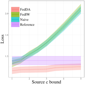
(a) Comparing all methods

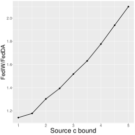
(b) Comparing FedIW and FedDA

Figure 1: Performances of methods with different covariate shifts. The horizontal axis represents the parameters of the source domains $c\in\{1,1.5,2,2.5,3,3.5,4,4.5,5\}$. (a) The vertical axis represents the mean of the performance of each method. (b) The vertical axis represents the ratio of the mean performance of FedIW to FedDA

From the results of Case 1 in Table 3, we can see that FedDA has the best mean performance with the smallest standard error in each situation. The results of Case 2 in Fig 1 indicate that FedDA significantly outperforms the other methods for every value of $c$. Fig. 1(a) shows that the advantage of FedDA becomes more and more strengthened when the covariate shifts between the target and sources become larger. The curve in Fig. 1(b) shows that FedDA outperforms FedIW to an increasing degree as the covariate shifts between the target and sources become larger. FedDA significantly outperforms Naive because FedDAE can well adapt to the FedCS setting, while the Naive method does not. FedDA also outperforms FedIW because FedDAE has a smaller asymptotic variance than FedIWE. Compared with Reference, FedDA performs better because it can make full use of additional source samples. These results are consistent with our theoretical analysis.

4 Real data Analysis

We verify the performance of our proposed method on a real dataset, Parkinson’s remote monitoring data.[26] The dataset consists of a series of biomedical voice measurement data from 42 patients with early Parkinson’s disease recruited to participate in a 6-month remote monitoring symptom progression test. These recordings were automatically recorded at the patients’ home. Here, we regard each patient’s home as a small hospital, and all the recordings of the patient are the data owned by this hospital. The columns of the dataset contain subject number, subject age, subject gender, time interval from baseline recruitment date, total UPDRS (Parkinson’s disease score scale) score, and 16 biomedical voice measurements. Each row corresponds to one of the 5875 voice records of these people. The primary purpose of the dataset is to predict the total UPDRS score from the 16 voice measurements.

We choose one hospital as the target and the others as the sources. The patient disease data of different source hospitals can not be fused. We use two models to train the data: the weighted least squares with exponential weight and the ridge regression. The hyperparameters are the flattening parameter of the weight and the regularization parameter, respectively. The loss function is square loss.

Experimental process: Use the target data without output values and the source data with output values; Divide the original target data into the training set and test set according to 7:3; Train the model on the training set of the target data and the source data; Predict the disease scores of the test set of the target data; Calculate the mean absolute error of the prediction as to the performance of the method used; Repeat the above steps 100 times with different random seeds.

Report the mean, standard error and worst-case performances of the 100 experimental results of the weighted least squares and the ridge regression in Table 4 and Table 4, respectively. The results indicate that FedDA is better than other methods in mean and worst-case with the smallest standard error.

Weighted least squares on real data Methods Mean Standard error Worst Case Naive 0.9003 0.0753 1.0862 FedIW 0.9519 0.0871 1.1573 FedDA 0.8578 0.0617 1.0034 Reference 0.8834 0.0657 1.0524

Ridge regression on real data Methods Mean Standard error Worst Case Naive 0.8645 0.0587 1.0072 FedIW 0.8694 0.0588 1.0121 FedDA 0.8468 0.0577 0.9848 Reference 0.8578 0.0684 1.0312

FedDA performs better than Naive because FedDAE can adapt to the FedCS setting between the hospitals. FedDA performs better than FedIW because FedDAE is stabler than FedIWE asymptotically. FedDA performs better than Reference because the samples of the source hospitals are more sufficient than that of the target hospital, and FedDA can make full use of existing data information.

5 Conclusion

This paper explores a new problem setting that extend the MS-CS setting under the framework of federated learning. The output values of the target data are completely missing, while the output values of the source data are available, and each source does not allow its data to leave its local area or be disclosed. To estimate the optimal hyperparameter, we first propose the federated importance weighting estimate of the target risk, which is asymptotically unbiased and can adapt to covariate shift. We further propose the federated domain adaptation estimate and show that it achieves the smaller asymptotic variance among a class of asymptotically unbiased estimates of the target risk. Then, we construct a weighted model by weighting all source models for the target task whose error can be bounded. Finally, we propose the federated covariate shift adaptation algorithm, a general and tractable hyperparameter optimization process. The experimental results indicate that our method is effective. However, our method does not take into account the nature of the under-sampled situation, which deserves further study in our future work.

Appendix A

A1. Lemma1 Consider $\{f_{n}(y)\}$ is a sequence of functions defined on the interval $[a,b]$. Suppose $f_{n}(y)$ converges uniformly to $f(y):[a,b]\to\mathbb{R}$ on $[a,b]$ as $n\to\infty$, then $\lim\limits_{n\to\infty}\underset{y\in[a,b]}{\min}f_{n}(y)=\underset{y\in[a,b]}{\min}f(y)$.

Proof: For any $\epsilon>0$, take $y_{0}\in[a,b]$ such that

$$f(y_{0})\leq\underset{y\in[a,b]}{\min}f(y)+\epsilon.$$ (11)

then since

$$f(y_{0})=\lim\limits_{n\to\infty}f_{n}(y_{0})\geq\lim\limits_{n\to\infty}\underset{y\in[a,b]}{\min}f_{n}(y),$$

let $\epsilon\to 0$ we get

$$\underset{y\in[a,b]}{\min}f(y)\geq\lim\limits_{n\to\infty}\underset{y\in[a,b]}{\min}f_{n}(y).$$ (12)

Take a positive constant $N$ such that $\forall n\geq N$, $|f_{n}(y)-f(y)|\leq\epsilon$ for any $y\in[a,b]$. This gives that $\forall n\geq N$,

$$-\epsilon\leq f_{n}(y)-f(y)\leq\epsilon,$$ (13)

$$-\epsilon\leq f_{n}(y_{0})-f(y_{0})\leq\epsilon.$$

From (13) we can obtain that

$$-2\epsilon\leq f_{n}(y)-f(y)+f(y_{0})-f_{n}(y_{0})\leq 2\epsilon$$

$$\implies f(y)-f_{n}(y)+f_{n}(y_{0})\leq f(y_{0})+2\epsilon.$$

Then

$$\underset{y\in[a,b]}{\min}f(y) =\underset{y\in[a,b]}{\min}[f(y)-f_{n}(y)+f_{n}(y)-f_{n}(y_{0})+f_{n}(y_{0})]$$

$$\leq\underset{y\in[a,b]}{\min}[f(y_{0})+2\epsilon+f_{n}(y)-f_{n}(y_{0})]$$

$$=\underset{y\in[a,b]}{\min}f_{n}(y)+f(y_{0})-f_{n}(y_{0})+2\epsilon$$

$$\leq\underset{y\in[a,b]}{\min}f_{n}(y)+3\epsilon.$$

Let $\epsilon\to 0$ and $n\to\infty$, we get

$$\underset{y\in[a,b]}{\min}f(y)\leq\lim\limits_{n\to\infty}\underset{y\in[a,b]}{\min}f_{n}(y).$$ (14)

Combine (12) and (14), $\lim\limits_{n\to\infty}\underset{y\in[a,b]}{\min}f_{n}(y)=\underset{y\in[a,b]}{\min}f(y).$

A2. Proof of Theorem 2.2
[(ii)]

For a given hyperparameter $\bm{\theta}\in\Theta$, $h\left(\bm{x};\bm{\omega},\bm{\theta}\right)\in\mathcal{Y}$ and $y\in\mathcal{Y}$ are both bounded, and $L$ satisfies the Lipschitz condition, so that

$$\mathbb{E}\Big{|}L\Big{(}h(\bm{x};\bm{\omega},\bm{\theta}),y\Big{)}\Big{|}<\infty.$$

$(\bm{x}_{j,1}^{tr},y_{j,1}^{tr}),\cdots,(\bm{x}_{j,n_{j}^{tr}}^{tr},y_{j,n_{j}^{tr}}^{tr})$ are i.i.d.$\sim p_{j}(\bm{x},y)$, Since $h$ and $L$ are continues and measurable, then for any given hyperparameter $\bm{\theta}\in\Theta$ and model parameter $\omega\in\Omega$,

$$L\Big{(}h(\bm{x}_{j,1}^{tr};\bm{\omega},\bm{\theta}),y_{j,1}^{tr}\Big{)},\cdots,L\Big{(}h(\bm{x}_{j,n_{j}^{tr}}^{tr};\bm{\omega},\bm{\theta}),y_{j,n_{j}^{tr}}^{tr}\Big{)}$$

are i.i.d. According to the weak law of large numbers, when $n_{j}^{tr}\to\infty$,

$$\frac{1}{n_{j}^{tr}}\sum_{i=1}^{n_{j}^{tr}}L\Big{(}h(\bm{x}_{j,i}^{tr};\bm{\omega},\bm{\theta}),y_{j,i}^{tr}\Big{)}\overset{P}{\to}\mathbb{E}_{(\bm{x},y)\sim p_{j}(\bm{x},y)}L\Big{(}h(\bm{x};\bm{\omega},\bm{\theta}),y\Big{)}.$$

For a given hyperparameter $\bm{\theta}\in\Theta$. Let

$$f_{n_{j}^{tr}}(\bm{\omega};D_{j}^{tr}) =\frac{1}{n_{j}^{tr}}\sum_{i=1}^{n_{j}^{tr}}L\Big{(}h(\bm{x}_{j,i}^{tr};\bm{\omega},\bm{\theta}),y_{j,i}^{tr}\Big{)},$$

$$f_{j}(\bm{\omega}) =\mathbb{E}_{(\bm{x},y)\sim p_{j}(\bm{x},y)}L\Big{(}h(\bm{x};\bm{\omega},\bm{\theta}),y\Big{)}.$$

Then $f_{n_{j}^{tr}}(\bm{\omega};D_{j}^{tr})\overset{P}{\to}f_{j}(\bm{\omega}),\forall\bm{\omega}\in\Omega$. For any $\epsilon_{1}>0$ and $\delta_{1}>0$, let

$$\tilde{G}_{j}=\cup\{D_{j}^{tr}:|f_{n_{j}^{tr}}(\bm{\omega};D_{j}^{tr})-f_{j}(\bm{\omega})|>\epsilon_{1},D_{j}^{tr}\sim p_{j}(\bm{x},y)\},$$

then $\exists N_{1}>0$, when $n_{j}^{tr}\geq N_{1}$, $\mu(\tilde{G}_{j})<\delta_{1}$. So that when $D_{j}^{tr}\subset\tilde{G}^{c}_{j}$, $f_{n_{j}^{tr}}(\bm{\omega};D_{j}^{tr})$ uniformly converges to $f_{j}(\bm{\omega})$ on $\Omega$. By Lemma1 in appendix A1 we have

$$\lim\limits_{n_{j}^{tr}\to\infty}\underset{\bm{\omega}\in\Omega}{\min}f_{n_{j}^{tr}}(\bm{\omega};D_{j}^{tr})=\underset{\bm{\omega}\in\Omega}{\min}f_{j}(\bm{\omega}).$$

Since the minimum value of $L$ about $\bm{\omega}$ is unique, then for any hyperparameter $\bm{\theta}\in\Theta$, when $D_{j}^{tr}\subset\tilde{G}^{c}_{j}$ and $n_{j}^{tr}\to\infty$,

$$\hat{\bm{\omega}}_{j}(\bm{\theta})=\underset{\bm{\omega}\in\Omega}{\arg\min}f_{n_{j}^{tr}}(\bm{\omega})\to\underset{\bm{\omega}\in\Omega}{\arg\min}f_{j}(\bm{\omega})={\bm{\omega}}_{j}(\bm{\theta}).$$

Since $h$ is continuous for $\bm{\omega}$ and $L$ is continuous, then when $D_{j}^{tr}\subset\tilde{G}^{c}_{j}$, for any $(\bm{x}_{j,i}^{val},y_{j,i}^{val})\in D_{j}^{val}$,

$$\lim_{n_{j}^{tr}\to\infty}L\Big{(}h\Big{(}\bm{x}_{j,i}^{val};\hat{\bm{\omega}}_{j}(\bm{\theta}),\bm{\theta}\Big{)},y_{j,i}^{val}\Big{)}=L\Big{(}h\Big{(}\bm{x}_{j,i}^{val};\bm{\omega}_{j}(\bm{\theta}),\bm{\theta}\Big{)},y_{j,i}^{val}\Big{)}.$$ (15)

According to Theorem 2 of Ref. kanamori2012statistical, we can obtain that when $n_{j}^{de},n_{T}\to\infty$, $\hat{r}_{j}(\cdot)\overset{P}{\to}r_{j}(\cdot)$, $j=1,2,\cdots,K.$ Here $\hat{r}_{j}(\cdot)$ is learned on $D_{j}^{de}$ and $D_{T}$. For any $\epsilon_{2}>0$ and $\delta_{2}>0$, let

$$\hat{G}_{j}=\cup\{D_{j}^{de}:|\hat{r}_{j}(\bm{x}_{j,i}^{val})-r_{j}(\bm{x}_{j,i}^{val})|>\epsilon_{2},D_{j}^{de}\sim p_{j}(\bm{x},y)\},$$

then $\exists N_{2}>0$, when $\min(n_{j}^{de},n_{T})\geq N_{2}$, $\mu(\hat{G}_{j})<\delta_{2}$. Let $G_{j}=\tilde{G}_{j}^{c}\cap\hat{G}_{j}^{c}$, then $G^{c}_{j}=\tilde{G}_{j}\cup\hat{G}_{j}$ and

$$\mu(G^{c}_{j})=1-\mu(G_{j})< 1-\max(\mu(\tilde{G}_{j}^{c}),\mu(\hat{G}_{j}^{c}))$$ (16)

$$= 1-\max(1-\mu(\tilde{G}_{j}),1-\mu(\hat{G}_{j}))$$

$$= \min(\mu(\tilde{G}_{j}),\mu(\hat{G}_{j}))$$

$$= \min(\delta_{1},\delta_{2}).$$

For any given hyperparameter $\bm{\theta}\in\Theta$, from (15) we obtain that for any $\epsilon_{3}>0$, $\exists N_{3}>0$, when $D_{j}^{tr}\subset G_{j}$ and $n_{j}^{tr}\geq N_{3}$,

$$\Big{|}L\Big{(}h\Big{(}\bm{x}_{j,i}^{val};\hat{\bm{\omega}}_{j}(\bm{\theta}),\bm{\theta}\Big{)},y_{j,i}^{val}\Big{)}-L\Big{(}h\Big{(}\bm{x}_{j,i}^{val};\bm{\omega}_{j}(\bm{\theta}),\bm{\theta}\Big{)},y_{j,i}^{val}\Big{)}\Big{|}<\epsilon_{3}.$$

Then, for any $(\bm{x},y)\in D_{j}^{val}$, when $D_{j}^{de}\subset G_{j}$ and $D_{j}^{tr}\subset G_{j}$, $\min(n_{j}^{de},n_{T})>N_{2}$ and $n_{j}^{tr}>N_{3}$,

$$\Big{|}\hat{r}_{j}(\bm{x})\cdot L\Big{(}h\Big{(}\bm{x};\hat{\bm{\omega}}_{j}(\bm{\theta}),\bm{\theta}\Big{)},y\Big{)}-r_{j}(\bm{x})\cdot L\Big{(}h\Big{(}\bm{x};\bm{\omega}_{j}(\bm{\theta}),\bm{\theta}\Big{)},y\Big{)}\Big{|}$$ (17)

$$= \Big{|}\hat{r}_{j}(\bm{x})\cdot L\Big{(}h\Big{(}\bm{x};\hat{\bm{\omega}}_{j}(\bm{\theta}),\bm{\theta}\Big{)},y\Big{)}-r_{j}(\bm{x})\cdot L\Big{(}h\Big{(}\bm{x};\hat{\bm{\omega}}_{j}(\bm{\theta}),\bm{\theta}\Big{)},y\Big{)}$$

$$+r_{j}(\bm{x})\cdot L\Big{(}h\Big{(}\bm{x};\hat{\bm{\omega}}_{j}(\bm{\theta}),\bm{\theta}\Big{)},y\Big{)}-r_{j}(\bm{x})\cdot L\Big{(}h\Big{(}\bm{x};\bm{\omega}_{j}(\bm{\theta}),\bm{\theta}\Big{)},y\Big{)}\Big{|}$$

$$\leq \Big{|}\hat{r}_{j}(\bm{x})-r_{j}(\bm{x})\Big{|}\cdot\Big{|}L\Big{(}h\Big{(}\bm{x};\hat{\bm{\omega}}_{j}(\bm{\theta}),\bm{\theta}\Big{)},y\Big{)}\Big{|}$$

$$+\Big{|}r_{j}(\bm{x})\Big{|}\cdot\Big{|}L\Big{(}h\Big{(}\bm{x};\hat{\bm{\omega}}_{j}(\bm{\theta}),\bm{\theta}\Big{)},y\Big{)}-L\Big{(}h\Big{(}\bm{x};\bm{\omega}_{j}(\bm{\theta}),\bm{\theta}\Big{)},y\Big{)}\Big{|}$$

$$\leq \epsilon_{2}\Big{|}L\Big{(}h\Big{(}\bm{x};\hat{\bm{\omega}}_{j}(\bm{\theta}),\bm{\theta}\Big{)},y\Big{)}\Big{|}+C\cdot\epsilon_{3}.$$

Let $\epsilon_{2}\to 0$ and $\epsilon_{3}\to 0$, then

$$\Big{|}\hat{r}_{j}(\bm{x})\cdot L\Big{(}h\Big{(}\bm{x};\hat{\bm{\omega}}_{j}(\bm{\theta}),\bm{\theta}\Big{)},y\Big{)}-r_{j}(\bm{x})\cdot L\Big{(}h\Big{(}\bm{x};\bm{\omega}_{j}(\bm{\theta}),\bm{\theta}\Big{)},y\Big{)}\Big{|}\to 0.$$

Form (16), we can obtain that for any $\delta_{4}>0$ and $\epsilon_{4}>0$, $\exists N_{4}>0$, when $n_{j}^{de},n_{j}^{tr},n_{T}\geq N_{4}$,

$$\mu\Big{(}\cup\Big{\{}D: \Big{|}\hat{r}_{j}(\bm{x})\cdot L\Big{(}h\Big{(}\bm{x};\hat{\bm{\omega}}_{j}(\bm{\theta}),\bm{\theta}\Big{)},y\Big{)}-r_{j}(\bm{x})\cdot L\Big{(}h\Big{(}\bm{x};\bm{\omega}_{j}(\bm{\theta}),\bm{\theta}\Big{)},y\Big{)}\Big{|}$$

$$>\epsilon_{4},D_{j}^{de}\sim p_{j}(\bm{x},y),D_{j}^{tr}\sim p_{j}(\bm{x},y),D=D_{j}^{de}\cup D_{j}^{tr}\Big{\}}\Big{)}=\mu(G_{j}^{c})<\delta_{4}.$$

Thus, for any given hyperparameter $\bm{\theta}\in\Theta$ and $(\bm{x},y)\in D_{j}^{val}$, when $n_{j}^{de},n_{j}^{tr},n_{T}\to\infty$,

$$\hat{r}_{j}(\bm{x})\cdot L\Big{(}h\Big{(}\bm{x};\hat{\bm{\omega}}_{j}(\bm{\theta}),\bm{\theta}\Big{)},y\Big{)}\overset{P}{\to}r_{j}(\bm{x})\cdot L\Big{(}h\Big{(}\bm{x};\bm{\omega}_{j}(\bm{\theta}),\bm{\theta}\Big{)},y\Big{)}.$$ (18)

So we have

$$\lim\limits_{n_{j}^{de},n_{j}^{tr},n_{T}\to\infty}\hat{f}_{IW}(\bm{\theta};D_{j})= \frac{1}{n_{j}^{val}}\sum_{i=1}^{n_{j}^{val}}\lim\limits_{n_{j}^{de},n_{j}^{tr},n_{T}\to\infty}\hat{r}_{j}(\bm{x}_{j,i}^{val})\cdot L\Big{(}h\Big{(}\bm{x}_{j,i}^{val};\hat{\bm{\omega}}_{j}(\bm{\theta}),\bm{\theta}\Big{)},y_{j,i}^{val}\Big{)}$$ (19)

$$= \frac{1}{n_{j}^{val}}\sum_{i=1}^{n_{j}^{val}}r_{j}(\bm{x}_{j,i}^{val})\cdot L\Big{(}h\Big{(}\bm{x}_{j,i}^{val};\bm{\omega}_{j}(\bm{\theta}),\bm{\theta}\Big{)},y_{j,i}^{val}\Big{)},$$

$$\mathbb{E}\lim\limits_{n_{j}^{de},n_{j}^{tr},n_{T}\to\infty}\hat{f}_{IW}(\bm{\theta};D_{j})= \frac{1}{n_{j}^{val}}\sum_{i=1}^{n_{j}^{val}}\mathbb{E}r_{j}(\bm{x}_{j,i}^{val})L\Big{(}h\Big{(}\bm{x}_{j,i}^{val};\bm{\omega}_{j}(\bm{\theta}),\bm{\theta}\Big{)},y_{j,i}^{val}\Big{)}$$

$$= \mathbb{E}\frac{p_{T}(\bm{x}_{j,1}^{val})}{p_{j}(\bm{x}_{j,1}^{val})}L\Big{(}h\Big{(}\bm{x}_{j,1}^{val};\bm{\omega}_{j}(\bm{\theta}),\bm{\theta}\Big{)},y_{j,1}^{val}\Big{)}$$

$$= \mathbb{E}\int_{\mathcal{X}}\frac{p_{T}(\bm{x})}{p_{j}(\bm{x})}L\Big{(}h\Big{(}\bm{x};\bm{\omega}_{j}(\bm{\theta}),\bm{\theta}\Big{)},y_{j,1}^{val}\Big{)}p_{j}(\bm{x})d\bm{x}$$

$$= \mathbb{E}\int_{\mathcal{X}}p_{T}(\bm{x})L\Big{(}h\Big{(}\bm{x};\bm{\omega}_{j}(\bm{\theta}),\bm{\theta}\Big{)},y_{j,1}^{val}\Big{)}d\bm{x}$$

$$\overset{(*)}{=} \mathbb{E}\int_{\mathcal{X}}L\Big{(}h\Big{(}\bm{t};\bm{\omega}_{j}(\bm{\theta}),\bm{\theta}\Big{)},u\Big{)}p_{T}(\bm{t})d\bm{t}$$

$$= \mathbb{E}L\Big{(}h\Big{(}\bm{t};\bm{\omega}(\bm{\theta}),\bm{\theta}\Big{)},u\Big{)}$$

$$= f_{T}(\bm{\theta}).$$

$(*)$ in (19) refers to Ref. 2000Improving and 2007Covariate. Since $\mathcal{Y}$ is bounded, $L$ satisfies the Lipschitz condition and $r(\cdot)\in[0,C]$ for a constant $C$, then $\lim\limits_{n_{j}^{de},n_{j}^{tr},n_{T}\to\infty}\hat{f}_{IW}(\bm{\theta};D_{j})$ is bounded. Thus, by the bounded convergence theorem, we have

$$\lim\limits_{n_{j}^{de},n_{j}^{tr},n_{T}\to\infty}\mathbb{E}\hat{f}_{IW}(\bm{\theta};D_{j})=\mathbb{E}\lim\limits_{n_{j}^{de},n_{j}^{tr},n_{T}\to\infty}\hat{f}_{IW}(\bm{\theta};D_{j})=f_{T}(\bm{\theta}).$$

The variance of $\hat{f}_{IW}$ is

$$\mathbb{V}\Big{[}\hat{f}_{IW}(\bm{\theta};D_{j})\Big{]}= \mathbb{V}_{(\bm{x},y)\sim p_{j}(\bm{x},y)}\Big{[}\hat{r}_{j}(\bm{x})L\Big{(}h\Big{(}\bm{x};\hat{\bm{\omega}}_{j}(\bm{\theta}),\bm{\theta}\Big{)},y\Big{)}\Big{]}$$

$$= \mathbb{E}_{(\bm{x},y)\sim p_{j}(\bm{x},y)}\Big{[}\hat{r}_{j}(\bm{x})L\Big{(}h\Big{(}\bm{x};\hat{\bm{\omega}}_{j}(\bm{\theta}),\bm{\theta}\Big{)},y\Big{)}\Big{]}^{2}$$

$$-\Big{\{}\mathbb{E}_{(\bm{x},y)\sim p_{j}(\bm{x},y)}\Big{[}\hat{r}_{j}(\bm{x})L\Big{(}h\Big{(}\bm{x};\hat{\bm{\omega}}_{j}(\bm{\theta}),\bm{\theta}\Big{)},y\Big{)}\Big{]}\Big{\}}^{2}.$$

By (18) and (19), according to the operation rules of limit and the bounded convergence theorem, we have

$$\lim\limits_{n_{j}^{de},n_{j}^{tr},n_{T}\to\infty}\mathbb{E}_{(\bm{x},y)\sim p_{j}(\bm{x},y)}\Big{[}\hat{r}_{j}(\bm{x})L\Big{(}h\Big{(}\bm{x};\hat{\bm{\omega}}_{j}(\bm{\theta}),\bm{\theta}\Big{)},y\Big{)}\Big{]}^{2}$$

$$= \mathbb{E}_{(\bm{x},y)\sim p_{j}(\bm{x},y)}\lim\limits_{n_{j}^{de},n_{j}^{tr},n_{T}\to\infty}\Big{[}\hat{r}_{j}(\bm{x})L\Big{(}h\Big{(}\bm{x};\hat{\bm{\omega}}_{j}(\bm{\theta}),\bm{\theta}\Big{)},y\Big{)}\Big{]}^{2}$$

$$= \mathbb{E}_{(\bm{x},y)\sim p_{j}(\bm{x},y)}\Big{[}\lim\limits_{n_{j}^{de},n_{j}^{tr},n_{T}\to\infty}\hat{r}_{j}(\bm{x})L\Big{(}h\Big{(}\bm{x};\hat{\bm{\omega}}_{j}(\bm{\theta}),\bm{\theta}\Big{)},y\Big{)}\Big{]}^{2}$$

$$= \mathbb{E}_{(\bm{x},y)\sim p_{j}(\bm{x},y)}\Big{[}r_{j}(\bm{x})L\Big{(}h\Big{(}\bm{x};\bm{\omega}_{j}(\bm{\theta}),\bm{\theta}\Big{)},y\Big{)}\Big{]}^{2}.$$

And by the same token, we can derive that

$$\lim\limits_{n_{j}^{de},n_{j}^{tr},n_{T}\to\infty}\Big{\{}\mathbb{E}_{(\bm{x},y)\sim p_{j}(\bm{x},y)}\Big{[}\hat{r}_{j}(\bm{x})L\Big{(}h\Big{(}\bm{x};\hat{\bm{\omega}}_{j}(\bm{\theta}),\bm{\theta}\Big{)},y\Big{)}\Big{]}\Big{\}}^{2}$$

$$= \Big{\{}\lim\limits_{n_{j}^{de},n_{j}^{tr},n_{T}\to\infty}\mathbb{E}_{(\bm{x},y)\sim p_{j}(\bm{x},y)}\Big{[}\hat{r}_{j}(\bm{x})L\Big{(}h\Big{(}\bm{x};\hat{\bm{\omega}}_{j}(\bm{\theta}),\bm{\theta}\Big{)},y\Big{)}\Big{]}\Big{\}}^{2}$$

$$= \Big{\{}\mathbb{E}_{(\bm{x},y)\sim p_{j}(\bm{x},y)}\lim\limits_{n_{j}^{de},n_{j}^{tr},n_{T}\to\infty}\Big{[}\hat{r}_{j}(\bm{x})L\Big{(}h\Big{(}\bm{x};\hat{\bm{\omega}}_{j}(\bm{\theta}),\bm{\theta}\Big{)},y\Big{)}\Big{]}\Big{\}}^{2}$$

$$= \Big{\{}\mathbb{E}_{(\bm{x},y)\sim p_{j}(\bm{x},y)}\Big{[}r_{j}(\bm{x})L\Big{(}h\Big{(}\bm{x};\bm{\omega}_{j}(\bm{\theta}),\bm{\theta}\Big{)},y\Big{)}\Big{]}\Big{\}}^{2}$$

$$= f^{2}_{T}(\bm{\theta}).$$

Thus,

$$\lim\limits_{n_{j}^{de},n_{j}^{tr},\atop n_{T}\to\infty}\mathbb{V}\Big{[}\hat{f}_{IW}(\bm{\theta};D_{j})\Big{]}= \mathbb{E}_{(\bm{x},y)\sim p_{j}(\bm{x},y)}\Big{[}r_{j}(\bm{x})L\Big{(}h\Big{(}\bm{x};\bm{\omega}_{j}(\bm{\theta}),\bm{\theta}\Big{)},y\Big{)}\Big{]}^{2}-f^{2}_{T}(\bm{\theta}).$$

∎

A2. Proof of Corollary 2.3

[(ii)]

Since $\hat{r}_{j}(\cdot)\to r_{j}(\cdot)$ a.s. when $n_{j}^{de}\to\infty$ and $n_{T}\to\infty$, by (LABEL:A11) and the asymptotic unbiasedness of the sample variance and sample covariance, we can obtain that

$$\lim\limits_{n_{j}^{de},n_{j}^{tr},n_{T}\to\infty}\widehat{\operatorname{Var}}\Big{[}\hat{r}_{j}(\bm{x}_{j}^{val})\Big{]}=\operatorname{Var}_{\bm{x}\sim p_{j}(\bm{x})}\Big{[}r_{j}(\bm{x})\Big{]},$$

$$\lim\limits_{n_{j}^{de},n_{j}^{tr},n_{T}\to\infty}\widehat{\operatorname{Cov}}\Big{[}\hat{r}_{j}(\bm{x}_{j}^{val})\cdot L\Big{(}h\big{(}\bm{x}_{j}^{val};\hat{\bm{\omega}}_{j}(\bm{\theta}),\bm{\theta}\big{)},y_{j}^{val}\Big{)},\hat{r}_{j}(\bm{x}_{j}^{val})\Big{]}$$

$$= \operatorname{Cov}_{(\bm{x},y)\sim p_{j}(\bm{x},y)}\Big{[}r_{j}(\bm{x})\cdot L\Big{(}h\big{(}\bm{x};\bm{\omega}_{j}(\bm{\theta}),\bm{\theta}\big{)},y\Big{)},r_{j}(\bm{x})\Big{]}.$$

Because $Var_{\bm{x}\sim p_{j}(\bm{x})}\left[r_{j}(\bm{x})\right]\neq 0$,

$$\lim\limits_{n_{j}^{de},n_{j}^{tr},n_{T}\to\infty}\frac{\widehat{\operatorname{Cov}}\Big{[}\hat{r}_{j}(\bm{x}_{j}^{val})\cdot L\Big{(}h\big{(}\bm{x}_{j}^{val};\hat{\bm{\omega}}_{j}(\bm{\theta}),\bm{\theta}\big{)},y_{j}^{val}\Big{)},\hat{r}_{j}(\bm{x}_{j}^{val})\Big{]}}{\widehat{\operatorname{Var}}\Big{[}\hat{r}_{j}(\bm{x}_{j}^{val})\Big{]}}$$

$$= \frac{\lim\limits_{n_{j}^{de},n_{j}^{tr},n_{T}\to\infty}\widehat{\operatorname{Cov}}\Big{[}\hat{r}_{j}(\bm{x}_{j}^{val})\cdot L\Big{(}h\big{(}\bm{x}_{j}^{val};\hat{\bm{\omega}}_{j}(\bm{\theta}),\bm{\theta}\big{)},y_{j}^{val}\Big{)},\hat{r}_{j}(\bm{x}_{j}^{val})\Big{]}}{\lim\limits_{n_{j}^{de},n_{j}^{tr},n_{T}\to\infty}\widehat{\operatorname{Var}}\Big{[}\hat{r}_{j}(\bm{x}_{j}^{val})\Big{]}}$$

$$= \frac{\operatorname{Cov}_{(\bm{x},y)\sim p_{j}(\bm{x},y)}\Big{[}r_{j}(\bm{x})\cdot L\Big{(}h\big{(}\bm{x};\bm{\omega}_{j}(\bm{\theta}),\bm{\theta}\big{)},y\Big{)},r_{j}(\bm{x})\Big{]}}{Var_{\bm{x}\sim p_{j}(\bm{x})}\Big{[}r_{j}(\bm{x})\Big{]}}.$$

Thus, we obtain that $\lim_{n_{j}^{de},n_{j}^{tr},n_{T}\to\infty}\hat{\eta}_{j}(\bm{\theta})=\eta_{j}(\bm{\theta}).$

Then, we have

$$\lim\limits_{n_{j}^{de},n_{j}^{tr},n_{T}\to\infty}\hat{f}_{CV}(\bm{\theta};D_{j})$$

$$= \lim\limits_{n_{j}^{de},n_{j}^{tr},\atop n_{T}\to\infty}\frac{1}{n_{j}^{val}}\sum_{i=1}^{n_{j}^{val}}\Big{[}\hat{r}_{j}(\bm{x}_{j,i}^{val})L\Big{(}h\Big{(}\bm{x}_{j,i}^{val};\hat{\bm{\omega}}_{j}(\bm{\theta}),\bm{\theta}\Big{)},y_{j,i}^{val}\Big{)}+\hat{\eta}_{j}(\bm{\theta})\cdot\Big{(}\hat{r}_{j}(x_{j,i}^{val})-1\Big{)}\Big{]}$$

$$= \frac{1}{n_{j}^{val}}\sum_{i=1}^{n_{j}^{val}}\lim\limits_{n_{j}^{de},n_{j}^{tr},\atop n_{T}\to\infty}\Big{[}\hat{r}_{j}(\bm{x}_{j,i}^{val})L\Big{(}h\Big{(}\bm{x}_{j,i}^{val};\hat{\bm{\omega}}_{j}(\bm{\theta}),\bm{\theta}\Big{)},y_{j,i}^{val}\Big{)}+\hat{\eta}_{j}(\bm{\theta})\cdot\Big{(}\hat{r}_{j}(x_{j,i}^{val})-1\Big{)}\Big{]}$$

$$= \frac{1}{n_{j}^{val}}\sum_{i=1}^{n_{j}^{val}}\Big{[}r_{j}(\bm{x}_{j,i}^{val})L\Big{(}h\Big{(}\bm{x}_{j,i}^{val};\bm{\omega}_{j}(\bm{\theta}),\bm{\theta}\Big{)},y_{j,i}^{val}\Big{)}+\eta_{j}(\bm{\theta})\cdot\Big{(}r_{j}(x_{j,i}^{val})-1\Big{)}\Big{]}.$$

Since

$$\mathbb{E}r_{j}(\bm{x})=\int_{\mathcal{X}}r_{j}(\bm{x})p_{j}(\bm{x})d\bm{x}=\int_{\mathcal{X}}\frac{p_{T}(\bm{x})}{p_{j}(\bm{x})}p_{j}(\bm{x})d\bm{x}=\int_{\mathcal{X}}p_{T}(\bm{x})d\bm{x}=1,$$

we can derive that

$$\mathbb{E}\lim\limits_{n_{j}^{de},n_{j}^{tr},n_{T}\to\infty}\hat{f}_{CV}(\bm{\theta};D_{j})$$ (20)

$$= \frac{1}{n_{j}^{val}}\sum_{i=1}^{n_{j}^{val}}\mathbb{E}\Big{[}r_{j}(\bm{x}_{j,i}^{val})L\Big{(}h\Big{(}\bm{x}_{j,i}^{val};\bm{\omega}_{j}(\bm{\theta}),\bm{\theta}\Big{)},y_{j,i}^{val}\Big{)}+\eta_{j}(\bm{\theta})\cdot\Big{(}r_{j}(x_{j,i}^{val})-1\Big{)}\Big{]}$$

$$= \mathbb{E}\Big{[}r_{j}(\bm{x}_{j,1}^{val})L\Big{(}h\Big{(}\bm{x}_{j,1}^{val};\bm{\omega}_{j}(\bm{\theta}),\bm{\theta}\Big{)},y_{j,1}^{val}\Big{)}+\eta_{j}(\bm{\theta})\cdot\Big{(}r_{j}(x_{j,1}^{val})-1\Big{)}\Big{]}$$

$$= \mathbb{E}\Big{[}r_{j}(\bm{x}_{j,1}^{val})L\Big{(}h\Big{(}\bm{x}_{j,1}^{val};\bm{\omega}_{j}(\bm{\theta}),\bm{\theta}\Big{)},y_{j,1}^{val}\Big{)}\Big{]}+\mathbb{E}\Big{[}\eta_{j}(\bm{\theta})\cdot\Big{(}r_{j}(x_{j,1}^{val})-1\Big{)}\Big{]}$$

$$\overset{(**)}{=} f_{T}(\bm{\theta})+\eta_{j}(\bm{\theta})\cdot\mathbb{E}\left[r_{j}(x_{j,1}^{val})-1\right]$$

$$= f_{T}(\bm{\theta}).$$

$(**)$ in (20) is derived from (19). Similar to the proof of Theorem 2.2 and by the bounded convergence theorem, we have

$$\lim\limits_{n_{j}^{de},n_{j}^{tr},n_{T}\to\infty}\mathbb{E}\hat{f}_{CV}(\bm{\theta};D_{j})=\mathbb{E}\lim\limits_{n_{j}^{de},n_{j}^{tr},n_{T}\to\infty}\hat{f}_{CV}(\bm{\theta};D_{j})=f_{T}(\bm{\theta}).$$

According to the operation rules of limit and the bounded convergence theorem, we have

$$\lim\limits_{n_{j}^{de},n_{j}^{tr},n_{T}\to\infty}\mathbb{V}\Big{[}\hat{f}_{CV}(\bm{\theta};D_{j})\Big{]}$$ (21)

$$= \lim\limits_{n_{j}^{de},n_{j}^{tr},n_{T}\to\infty}\mathbb{E}\Big{[}\hat{f}_{CV}(\bm{\theta};D_{j})\Big{]}^{2}-\lim\limits_{n_{j}^{de},n_{j}^{tr},n_{T}\to\infty}\Big{\{}\mathbb{E}\Big{[}\hat{f}_{CV}(\bm{\theta};D_{j})\Big{]}\Big{\}}^{2}$$

$$= \mathbb{E}\lim\limits_{n_{j}^{de},n_{j}^{tr},n_{T}\to\infty}\Big{[}\hat{f}_{CV}(\bm{\theta};D_{j})\Big{]}^{2}-\Big{\{}\lim\limits_{n_{j}^{de},n_{j}^{tr},n_{T}\to\infty}\mathbb{E}\Big{[}\hat{f}_{CV}(\bm{\theta};D_{j})\Big{]}\Big{\}}^{2}$$

$$= \mathbb{E}\Big{[}\lim\limits_{n_{j}^{de},n_{j}^{tr},n_{T}\to\infty}\hat{f}_{CV}(\bm{\theta};D_{j})\Big{]}^{2}-f_{T}^{2}(\bm{\theta})$$

$$= \mathbb{E}\Big{\{}\frac{1}{n_{j}^{val}}\sum_{i=1}^{n_{j}^{val}}\Big{[}r_{j}(\bm{x}_{j,i}^{val})L\Big{(}h\Big{(}\bm{x}_{j,i}^{val};\bm{\omega}_{j}(\bm{\theta}),\bm{\theta}\Big{)},y_{j,i}^{val}\Big{)}+\eta_{j}(\bm{\theta})\cdot\Big{(}r_{j}(\bm{x}_{j,i}^{val})-1\Big{)}\Big{]}\Big{\}}^{2}$$

$$-f_{T}^{2}(\bm{\theta})$$

$$= \frac{1}{n_{j}^{val}}\Big{\{}\mathbb{E}_{(\bm{x},y)\sim p_{j}(\bm{x},y)}\Big{[}r_{j}(\bm{x})L\Big{(}h\Big{(}\bm{x};\bm{\omega}_{j}(\bm{\theta}),\bm{\theta}\Big{)},y\Big{)}+\eta_{j}(\bm{\theta})\cdot\Big{(}r_{j}(\bm{x})-1\Big{)}\Big{]}^{2}$$

$$\quad\quad\quad-f_{T}^{2}(\bm{\theta})\Big{\}}$$

To derive the last equation of (21), let $Z,Z_{1},\cdots,Z_{n}$ be i.i.d. random variables,

$$\mathbb{E}\Big{[}\frac{1}{n}\sum_{i=1}^{n}Z_{i}\Big{]}^{2}-(\mathbb{E}Z)^{2}=\frac{1}{n^{2}}\mathbb{E}\Big{[}\sum_{i=1}^{n}Z_{i}^{2}+2\sum_{i<j}Z_{i}Z_{j}\Big{]}-(\mathbb{E}Z)^{2}$$

$$= \frac{1}{n}\mathbb{E}Z^{2}+\frac{2}{n^{2}}\frac{n(n-1)}{2}(\mathbb{E}Z)^{2}-(\mathbb{E}Z)^{2}=\frac{1}{n}[\mathbb{E}Z^{2}-(\mathbb{E}Z)^{2}].$$

By the same token, we have

$$\lim\limits_{n_{j}^{de},n_{j}^{tr},n_{T}\to\infty}\mathbb{V}\Big{[}\hat{f}_{IW}(\bm{\theta};D_{j})\Big{]}$$

$$= \frac{1}{n_{j}^{val}}\Big{\{}\mathbb{E}_{(\bm{x},y)\sim p_{j}(\bm{x},y)}\Big{[}r_{j}(\bm{x})L\Big{(}h\Big{(}\bm{x};\bm{\omega}_{j}(\bm{\theta}),\bm{\theta}\Big{)},y\Big{)}\Big{]}^{2}-f^{2}_{T}(\bm{\theta})\Big{\}}.$$

The control variate method[12] implies that

$$\mathbb{E}\Big{[}r_{j}(\bm{x})L\Big{(}h\Big{(}\bm{x};\bm{\omega}_{j}(\bm{\theta}),\bm{\theta}\Big{)},y\Big{)}+\eta_{j}(\bm{\theta})\cdot\Big{(}r_{j}(x)-1\Big{)}\Big{]}^{2}$$

$$\leq \mathbb{E}\Big{[}r_{j}(\bm{x})L\Big{(}h\Big{(}\bm{x};\bm{\omega}_{j}(\bm{\theta}),\bm{\theta}\Big{)},y\Big{)}\Big{]}^{2},$$

so we have

$$\lim\limits_{n_{j}^{de},n_{j}^{tr},n_{T}\to\infty}\mathbb{V}\Big{[}\hat{f}_{CV}(\bm{\theta};D_{j})\Big{]}\leq\lim\limits_{n_{j}^{de},n_{j}^{tr},n_{T}\to\infty}\mathbb{V}\Big{[}\hat{f}_{IW}(\bm{\theta};D_{j})\Big{]}.$$

∎

A3. Proof of Corollary 2.6

[(ii)]

For a given hyperparameter $\bm{\theta}\in\Theta$ and any set of weights for sources $\bm{\lambda}=\{\lambda_{1},\cdots,\lambda_{K}\}$,

$$\lim\limits_{\forall j,n_{j}^{de},n_{j}^{tr},n_{T}\to\infty}\hat{f}_{\bm{\lambda}}\Big{(}\bm{\theta};\{D_{j}\}_{j=1}^{K}\Big{)}=\sum_{j=1}^{K}\lambda_{j}n_{j}^{val}\cdot\lim\limits_{n_{j}^{de},n_{j}^{tr},n_{T}\to\infty}\hat{f}_{CV}(\bm{\theta};D_{j}).$$

Similar to the proof of Theorem 2.2, we can obtain that

$$\lim\limits_{\forall j,n_{j}^{de},n_{j}^{tr},n_{T}\to\infty}\mathbb{E}\hat{f}_{\bm{\lambda}}\Big{(}\bm{\theta};\{D_{j}\}_{j=1}^{K}\Big{)}=\mathbb{E}\lim\limits_{\forall j,n_{j}^{de},n_{j}^{tr},n_{T}\to\infty}\hat{f}_{\bm{\lambda}}\Big{(}\bm{\theta};\{D_{j}\}_{j=1}^{K}\Big{)}$$

$$= \sum_{j=1}^{K}\lambda_{j}n_{j}^{val}\cdot\mathbb{E}\lim\limits_{n_{j}^{de},n_{j}^{tr},n_{T}\to\infty}\hat{f}_{CV}(\bm{\theta};D_{j})=\sum_{j=1}^{K}\lambda_{j}n_{j}^{val}\cdot f_{T}(\bm{\theta})=f_{T}(\bm{\theta}).$$

We can see that $\hat{f}_{FedDA}\left(\bm{\theta};\{D_{j}\}_{j=1}^{K}\right)$ is a special case of $\hat{f}_{\bm{\lambda}}\left(\bm{\theta};\{D_{j}\}_{j=1}^{K}\right)$ where $\lambda_{j}=\hat{\lambda}_{j}(\bm{\theta}),j=1,2,\cdots,K$, so

$$\lim\limits_{\forall j,n_{j}^{de},n_{j}^{tr},n_{T}\to\infty}\mathbb{E}\hat{f}_{FedDA}\Big{(}\bm{\theta};\{D_{j}\}_{j=1}^{K}\Big{)}=f_{T}(\bm{\theta}).$$

Because $K$ source datasets are independent and each source dataset is i.i.d., we have

$$\mathbb{V}\Big{[}\hat{f}_{\bm{\lambda}}\Big{(}\bm{\theta};\{D_{j}\}_{j=1}^{K}\Big{)}\Big{]}=\sum_{j=1}^{K}\mathbb{V}\Big{[}\lambda_{j}n_{j}^{val}\hat{f}_{CV}(\bm{\theta};D_{j})\Big{]}=\sum_{j=1}^{K}\lambda_{j}^{2}(n_{j}^{val})^{2}\mathbb{V}\Big{[}\hat{f}_{CV}(\bm{\theta};D_{j})\Big{]}.$$

According to the expression of $\operatorname{Div}_{j}\left(\bm{\theta}\right)$ and (21), we can obtain that

$$\lim\limits_{n_{j}^{de},n_{j}^{tr},n_{T}\to\infty}\mathbb{V}\Big{[}\hat{f}_{CV}(\bm{\theta};D_{j})\Big{]}=\frac{1}{n_{j}^{val}}\operatorname{Div}_{j}\left(\bm{\theta}\right),$$

Then, by the operation rules of limit

$$\lim\limits_{\forall j,n_{j}^{de},n_{j}^{tr},\atop n_{j}^{val},n_{T}\to\infty}\mathbb{V}\Big{[}\hat{f}_{\bm{\lambda}}\Big{(}\bm{\theta};\{D_{j}\}_{j=1}^{K}\Big{)}\Big{]}$$

$$= \lim\limits_{\forall j,n_{j}^{de},n_{j}^{tr},\atop n_{j}^{val},n_{T}\to\infty}\sum_{j=1}^{K}\lambda_{j}^{2}(n_{j}^{val})^{2}\lim\limits_{n_{j}^{de},n_{j}^{tr},n_{T}\to\infty}\mathbb{V}\Big{[}\hat{f}_{CV}(\bm{\theta};D_{j})\Big{]}$$

$$= \lim\limits_{\forall j,n_{j}^{de},n_{j}^{tr},\atop n_{j}^{val},n_{T}\to\infty}\sum_{j=1}^{K}\lambda_{j}^{2}n_{j}^{val}\operatorname{Div}_{j}\left(\bm{\theta}\right).$$

To investigate the asymptotic variance of FedDAE, we first study the limit of $\hat{\lambda}_{j}(\bm{\theta})$, $j=1,2,\cdots,K$. According to the operation rules of limit, we have

$$\lim\limits_{n_{j}^{de},n_{j}^{tr},n_{T}\to\infty}\widehat{\operatorname{Div}}_{j}\left(\bm{\theta}\right)$$

$$= \frac{1}{n_{j}^{val}}\sum_{i=1}^{n_{j}^{val}}\lim\limits_{n_{j}^{de},n_{j}^{tr},n_{T}\to\infty}\Big{[}\hat{r}_{j}(\bm{x}_{j,i}^{val})\cdot L\Big{(}h\Big{(}\bm{x}_{j,i}^{val};\hat{\bm{\omega}}_{j}(\bm{\theta}),\bm{\theta}\Big{)},y_{j,i}^{val}\Big{)}$$

$$\quad\quad\quad\quad\quad\quad\quad\quad\quad\quad+\hat{\eta}_{j}(\bm{\theta})\cdot\Big{(}\hat{r}_{j}(\bm{x}_{j,i}^{val})-1\Big{)}\Big{]}^{2}$$

$$-\lim\limits_{n_{j}^{de},n_{j}^{tr},n_{T}\to\infty}\Big{[}\frac{1}{n_{j}^{val}}\sum_{i=1}^{n_{j}^{val}}\Big{(}\hat{r}_{j}(\bm{x}_{j,i}^{val})\cdot L\Big{(}h\Big{(}\bm{x}_{j,i}^{val};\hat{\bm{\omega}}_{j}(\bm{\theta}),\bm{\theta}\Big{)},y_{j,i}^{val}\Big{)}$$

$$\quad\quad\quad\quad\quad\quad\quad+\hat{\eta}_{j}(\bm{\theta})\cdot\Big{(}\hat{r}_{j}(\bm{x}_{j,i}^{val})-1\Big{)}\Big{)}\Big{]}^{2}$$

$$= \frac{1}{n_{j}^{val}}\sum_{i=1}^{n_{j}^{val}}\Big{[}r_{j}(\bm{x}_{j,i}^{val})\cdot L\Big{(}h\Big{(}\bm{x}_{j,i}^{val};\bm{\omega}_{j}(\bm{\theta}),\bm{\theta}\Big{)},y_{j,i}^{val}\Big{)}+\eta_{j}(\bm{\theta})\cdot\Big{(}r_{j}(\bm{x}_{j,i}^{val})-1\Big{)}\Big{]}^{2}$$

$$-\Big{[}\frac{1}{n_{j}^{val}}\sum_{i=1}^{n_{j}^{val}}\Big{(}r_{j}(\bm{x}_{j,i}^{val})\cdot L\Big{(}h\Big{(}\bm{x}_{j,i}^{val};\bm{\omega}_{j}(\bm{\theta}),\bm{\theta}\Big{)},y_{j,i}^{val}\Big{)}+\eta_{j}(\bm{\theta})\cdot\Big{(}r_{j}(\bm{x}_{j,i}^{val})-1\Big{)}\Big{)}\Big{]}^{2}.$$

Since $\eta_{j}(\bm{\theta})$ is bounded, we can use strong law of large numbers and the operation rules of limit to obtain that

$$\lim\limits_{n_{j}^{de},n_{j}^{tr},n_{j}^{val},n_{T}\to\infty}\widehat{\operatorname{Div}}_{j}\left(\bm{\theta}\right)$$

$$= \lim\limits_{n_{j}^{val}\to\infty}\frac{1}{n_{j}^{val}}\sum_{i=1}^{n_{j}^{val}}\Big{[}r_{j}(\bm{x}_{j,i}^{val})\cdot L\Big{(}h\Big{(}\bm{x}_{j,i}^{val};\bm{\omega}_{j}(\bm{\theta}),\bm{\theta}\Big{)},y_{j,i}^{val}\Big{)}$$

$$\quad\quad\quad\quad\quad\quad\quad\quad+\eta_{j}(\bm{\theta})\cdot\Big{(}r_{j}(\bm{x}_{j,i}^{val})-1\Big{)}\Big{]}^{2}$$

$$-\lim\limits_{n_{j}^{val}\to\infty}\Big{[}\frac{1}{n_{j}^{val}}\sum_{i=1}^{n_{j}^{val}}\Big{(}r_{j}(\bm{x}_{j,i}^{val})\cdot L\Big{(}h\Big{(}\bm{x}_{j,i}^{val};\bm{\omega}_{j}(\bm{\theta}),\bm{\theta}\Big{)},y_{j,i}^{val}\Big{)}$$

$$\quad\quad\quad\quad\quad+\eta_{j}(\bm{\theta})\cdot\Big{(}r_{j}(\bm{x}_{j,i}^{val})-1\Big{)}\Big{)}\Big{]}^{2}$$

$$= \mathbb{E}_{(\bm{x},y)\sim p_{j}(\bm{x},y)}\Big{[}r_{j}(\bm{x})\cdot L\Big{(}h\Big{(}\bm{x};\bm{\omega}_{j}(\bm{\theta}),\bm{\theta}\Big{)},y\Big{)}+\eta_{j}(\bm{\theta})\cdot\Big{(}r_{j}(\bm{x})-1\Big{)}\Big{]}^{2}$$

$$-\Big{\{}\lim\limits_{n_{j}^{val}\to\infty}\frac{1}{n_{j}^{val}}\sum_{i=1}^{n_{j}^{val}}\Big{(}r_{j}(\bm{x}_{j,i}^{val})\cdot L\Big{(}h\Big{(}\bm{x}_{j,i}^{val};\bm{\omega}_{j}(\bm{\theta}),\bm{\theta}\Big{)},y_{j,i}^{val}\Big{)}$$

$$\quad\quad+\eta_{j}(\bm{\theta})\cdot\Big{(}r_{j}(\bm{x}_{j,i}^{val})-1\Big{)}\Big{)}\Big{\}}^{2}$$

$$= \mathbb{E}_{(\bm{x},y)\sim p_{j}(\bm{x},y)}\Big{[}r_{j}(\bm{x})\cdot L\Big{(}h\Big{(}\bm{x};\bm{\omega}_{j}(\bm{\theta}),\bm{\theta}\Big{)},y\Big{)}+\eta_{j}(\bm{\theta})\cdot\Big{(}r_{j}(\bm{x})-1\Big{)}\Big{]}^{2}$$

$$-\Big{\{}\mathbb{E}_{(\bm{x},y)\sim p_{j}(\bm{x},y)}\Big{[}r_{j}(\bm{x})\cdot L\Big{(}h\Big{(}\bm{x};\bm{\omega}_{j}(\bm{\theta}),\bm{\theta}\Big{)},y\Big{)}+\eta_{j}(\bm{\theta})\cdot\Big{(}r_{j}(\bm{x})-1\Big{)}\Big{]}\Big{\}}^{2}$$

$$= \mathbb{E}_{(\bm{x},y)\sim p_{j}(\bm{x},y)}\Big{[}r_{j}(\bm{x})\cdot L\Big{(}h\Big{(}\bm{x};\bm{\omega}_{j}(\bm{\theta}),\bm{\theta}\Big{)},y\Big{)}+\eta_{j}(\bm{\theta})\cdot\Big{(}r_{j}(\bm{x})-1\Big{)}\Big{]}^{2}-f^{2}_{T}(\bm{\theta})$$

$$= \operatorname{Div}_{j}\left(\bm{\theta}\right).$$

According to the operation rules of limit, we can derive that

$$\lim\limits_{\forall j,n_{j}^{de},n_{j}^{tr},n_{j}^{val},n_{T}\to\infty}\hat{\lambda}_{j}(\bm{\theta})$$

$$= \lim\limits_{\forall j,n_{j}^{de},n_{j}^{tr},n_{j}^{val},n_{T}\to\infty}\Bigg{(}\widehat{\operatorname{Div}}_{j}\left(\bm{\theta}\right)\sum_{j=1}^{K}\frac{n_{j}^{val}}{\widehat{\operatorname{Div}}_{j}\left(\bm{\theta}\right)}\Bigg{)}^{-1}$$

$$= \Bigg{(}\lim\limits_{\forall j,n_{j}^{de},n_{j}^{tr},n_{j}^{val},n_{T}\to\infty}\widehat{\operatorname{Div}}_{j}\left(\bm{\theta}\right)\sum_{j=1}^{K}\frac{n_{j}^{val}}{\widehat{\operatorname{Div}}_{j}\left(\bm{\theta}\right)}\Bigg{)}^{-1}$$

$$= \Bigg{(}\operatorname{Div}_{j}\left(\bm{\theta}\right)\sum_{j=1}^{K}\frac{n_{j}^{val}}{\operatorname{Div}_{j}\left(\bm{\theta}\right)}\Bigg{)}^{-1}$$

$$= \lambda_{j}(\bm{\theta}).$$

And by the same token, we have

$$\lim\limits_{\forall j,n_{j}^{de},n_{j}^{tr},n_{j}^{val},n_{T}\to\infty}\mathbb{V}\Big{[}\hat{f}_{FedDA}\Big{(}\bm{\theta};\{D_{j}\}_{j=1}^{K}\Big{)}\Big{]}$$

$$= \lim\limits_{\forall j,n_{j}^{de},n_{j}^{tr},n_{j}^{val},n_{T}\to\infty}\sum_{j=1}^{K}\hat{\lambda}_{j}(\bm{\theta})^{2}(n_{j}^{val})^{2}\mathbb{V}\Big{[}\hat{f}_{CV}(\bm{\theta};D_{j})\Big{]}$$

$$= \lim\limits_{\forall j,n_{j}^{val}\to\infty}\sum_{j=1}^{K}\lambda_{j}^{2}(\bm{\theta})n_{j}^{val}\operatorname{Div}_{j}\left(\bm{\theta}\right)$$

$$= \lim\limits_{\forall j,n_{j}^{val}\to\infty}\sum_{j=1}^{K}\Bigg{(}\operatorname{Div}_{j}\left(\bm{\theta}\right)\sum_{j=1}^{K}\frac{n_{j}^{val}}{\operatorname{Div}_{j}\left(\bm{\theta}\right)}\Bigg{)}^{-2}n_{j}^{val}\operatorname{Div}_{j}\left(\bm{\theta}\right)$$

$$= \lim\limits_{\forall j,n_{j}^{val}\to\infty}\Bigg{(}\sum_{j=1}^{K}\frac{n_{j}^{val}}{\operatorname{Div}_{j}\left(\bm{\theta}\right)}\Bigg{)}\Bigg{(}\sum_{j=1}^{K}\frac{n_{j}^{val}}{\operatorname{Div}_{j}\left(\bm{\theta}\right)}\Bigg{)}^{-2}$$

$$= \lim\limits_{\forall j,n_{j}^{val}\to\infty}\Bigg{(}\sum_{j=1}^{K}\frac{n_{j}^{val}}{\operatorname{Div}_{j}\left(\bm{\theta}\right)}\Bigg{)}^{-1}.$$

Then, for any given set of weights of sources $\bm{\lambda}=\{\lambda_{1},\cdots,\lambda_{K}\}$, we can use the Cauchy-Schwarz inequality to obtain that,

$$1=\Bigg{(}\sum_{j=1}^{K}\lambda_{j}n_{j}^{val}\Bigg{)}^{2}\leq\Bigg{(}\sum_{j=1}^{K}\lambda_{j}^{2}n_{j}^{val}\operatorname{Div}_{j}\left(\bm{\theta}\right)\Bigg{)}\Bigg{(}\sum_{j=1}^{K}\frac{n_{j}^{val}}{\operatorname{Div}_{j}\left(\bm{\theta}\right)}\Bigg{)}$$

$$\implies\Bigg{(}\sum_{j=1}^{K}\frac{n_{j}^{val}}{\operatorname{Div}_{j}\left(\bm{\theta}\right)}\Bigg{)}^{-1}\leq\Bigg{(}\sum_{j=1}^{K}\lambda_{j}^{2}n_{j}^{val}\operatorname{Div}_{j}\left(\bm{\theta}\right)\Bigg{)}$$

$$\implies\lim\limits_{\forall j,n_{j}^{val}\to\infty}\Bigg{(}\sum_{j=1}^{K}\frac{n_{j}^{val}}{\operatorname{Div}_{j}\left(\bm{\theta}\right)}\Bigg{)}^{-1}\leq\lim\limits_{\forall j,n_{j}^{val}\to\infty}\Bigg{(}\sum_{j=1}^{K}\lambda_{j}^{2}n_{j}^{val}\operatorname{Div}_{j}\left(\bm{\theta}\right)\Bigg{)}$$

$$\implies\lim\limits_{\forall j,n_{j}^{de},n_{j}^{tr},\atop n_{j}^{val},n_{T}\to\infty}\mathbb{V}\Big{[}\hat{f}_{FedDA}\Big{(}\bm{\theta};\{D_{j}\}_{j=1}^{K}\Big{)}\Big{]}\leq\lim\limits_{\forall j,n_{j}^{de},n_{j}^{tr},\atop n_{j}^{val},n_{T}\to\infty}\mathbb{V}\Big{[}\hat{f}_{\bm{\lambda}}\Big{(}\bm{\theta};\{D_{j}\}_{j=1}^{K}\Big{)}\Big{]}.$$

∎

A4. Proof of Corollary 2.7

Let $\tilde{\bm{\lambda}}$ be a set of weights for sources with $\tilde{\lambda}_{j}=1/n^{val},j=1,2,\cdots,K$, it is easily to prove that $\tilde{\bm{\lambda}}$ satisfies $\tilde{\lambda}_{j}\geq 0,j=1,2,\cdots,K$ and $\sum_{j=1}^{K}\tilde{\lambda}_{j}n_{j}^{val}=1$. Then, by Corollary 2.6 we can derive that

$$\lim\limits_{\forall j,n_{j}^{de},n_{j}^{tr},\atop n_{j}^{val},n_{T}\to\infty}\mathbb{V}\Big{[}\hat{f}_{FedDA}\Big{(}\bm{\theta};\{D_{j}\}_{j=1}^{K}\Big{)}\Big{]}\leq\lim\limits_{\forall j,n_{j}^{de},n_{j}^{tr},\atop n_{j}^{val},n_{T}\to\infty}\mathbb{V}\Big{[}\hat{f}_{\tilde{\bm{\lambda}}}\Big{(}\bm{\theta};\{D_{j}\}_{j=1}^{K}\Big{)}\Big{]},$$

where

$$\hat{f}_{\tilde{\bm{\lambda}}}\Big{(}\bm{\theta};\{D_{j}\}_{j=1}^{K}\Big{)}=\sum_{j=1}^{K}\tilde{\lambda}_{j}n_{j}^{val}\hat{f}_{CV}(\bm{\theta};D_{j})=\frac{1}{n^{val}}\sum_{j=1}^{K}n_{j}^{val}\cdot\hat{f}_{CV}(\bm{\theta};D_{j}).$$

According to (4) and the inequality in Corollary 2.3, we have

$$\lim\limits_{\forall j,n_{j}^{de},n_{j}^{tr},\atop n_{j}^{val},n_{T}\to\infty}\mathbb{V}\Big{[}\hat{f}_{\tilde{\bm{\lambda}}}\Big{(}\bm{\theta};\{D_{j}\}_{j=1}^{K}\Big{)}\Big{]}\leq\lim\limits_{\forall j,n_{j}^{de},n_{j}^{tr},\atop n_{j}^{val},n_{T}\to\infty}\mathbb{V}\Big{[}\hat{f}_{FedIW}\Big{(}\bm{\theta};\{D_{j}\}_{j=1}^{K}\Big{)}\Big{]}.$$

Thus, we obtain

$$\lim\limits_{\forall j,n_{j}^{de},n_{j}^{tr},\atop n_{j}^{val},n_{T}\to\infty}\mathbb{V}\Big{[}\hat{f}_{FedDA}\Big{(}\bm{\theta};\{D_{j}\}_{j=1}^{K}\Big{)}\Big{]}\leq\lim\limits_{\forall j,n_{j}^{de},n_{j}^{tr},\atop n_{j}^{val},n_{T}\to\infty}\mathbb{V}\Big{[}\hat{f}_{FedIW}\Big{(}\bm{\theta};\{D_{j}\}_{j=1}^{K}\Big{)}\Big{]}.$$

∎

References

• [1] Shai Ben-David, John Blitzer, Koby Crammer, Alex Kulesza, Fernando Pereira, and Jennifer Wortman Vaughan. A theory of learning from different domains. Machine learning, 79(1):151–175, 2010.
• [2] James Bergstra, Rémi Bardenet, Yoshua Bengio, and Balázs Kégl. Algorithms for hyper-parameter optimization. In J. Shawe-Taylor, R. Zemel, P. Bartlett, F. Pereira, and K. Q. Weinberger, editors, Advances in Neural Information Processing Systems, volume 24. Curran Associates, Inc., 2011.
• [3] John Blitzer, Koby Crammer, Alex Kulesza, Fernando Pereira, and Jennifer Wortman. Learning bounds for domain adaptation. Advances in neural information processing systems, 20, 2007.
• [4] Keith Bonawitz, Vladimir Ivanov, Ben Kreuter, Antonio Marcedone, H Brendan McMahan, Sarvar Patel, Daniel Ramage, Aaron Segal, and Karn Seth. Practical secure aggregation for privacy-preserving machine learning. In proceedings of the 2017 ACM SIGSAC Conference on Computer and Communications Security, pages 1175–1191, 2017.
• [5] Edwin V Bonilla, Kian Chai, and Christopher Williams. Multi-task gaussian process prediction. Advances in neural information processing systems, 20, 2007.
• [6] Víctor Elvira, Luca Martino, David Luengo, and Mónica F Bugallo. Efficient multiple importance sampling estimators. IEEE Signal Processing Letters, 22(10):1757–1761, 2015.
• [7] Matthias Feurer and Frank Hutter. Hyperparameter optimization. In Automated machine learning, pages 3–33. Springer, Cham, 2019.
• [8] Matthias Feurer, Benjamin Letham, Frank Hutter, and Eytan Bakshy. Practical transfer learning for bayesian optimization. arXiv preprint arXiv:1802.02219, 2018.
• [9] Ran Gilad-Bachrach, Nathan Dowlin, Kim Laine, Kristin Lauter, Michael Naehrig, and John Wernsing. Cryptonets: Applying neural networks to encrypted data with high throughput and accuracy. In International conference on machine learning, pages 201–210. PMLR, 2016.
• [10] Takafumi Kanamori, Shohei Hido, and Masashi Sugiyama. A least-squares approach to direct importance estimation. The Journal of Machine Learning Research, 10:1391–1445, 2009.
• [11] Takafumi Kanamori, Taiji Suzuki, and Masashi Sugiyama. Statistical analysis of kernel-based least-squares density-ratio estimation. Machine Learning, 86(3):335–367, 2012.
• [12] Christiane Lemieux. Control Variates. American Cancer Society, 2017.
• [13] Yang Liu, Yan Kang, Chaoping Xing, Tianjian Chen, and Qiang Yang. A secure federated transfer learning framework. IEEE Intelligent Systems, 35(4):70–82, 2020.
• [14] Mingsheng Long, Zhangjie Cao, Jianmin Wang, and Michael I Jordan. Conditional adversarial domain adaptation. Advances in neural information processing systems, 31, 2018.
• [15] Payman Mohassel and Peter Rindal. Aby3: A mixed protocol framework for machine learning. In Proceedings of the 2018 ACM SIGSAC conference on computer and communications security, pages 35–52, 2018.
• [16] Payman Mohassel and Yupeng Zhang. Secureml: A system for scalable privacy-preserving machine learning. In 2017 IEEE symposium on security and privacy (SP), pages 19–38. IEEE, 2017.
• [17] Masahiro Nomura and Yuta Saito. Efficient hyperparameter optimization under multi-source covariate shift. In Proceedings of the 30th ACM International Conference on Information & Knowledge Management, pages 1376–1385, 2021.
• [18] Sinno Jialin Pan and Qiang Yang. A survey on transfer learning. IEEE Transactions on knowledge and data engineering, 22(10):1345–1359, 2009.
• [19] Xingchao Peng, Zijun Huang, Yizhe Zhu, and Kate Saenko. Federated adversarial domain adaptation. arXiv preprint arXiv:1911.02054, 2019.
• [20] Xingchao Peng, Zijun Huang, Yizhe Zhu, and Kate Saenko. Federated adversarial domain adaptation. arXiv preprint arXiv:1911.02054, 2019.
• [21] Valerio Perrone, Rodolphe Jenatton, Matthias W Seeger, and Cédric Archambeau. Scalable hyperparameter transfer learning. Advances in neural information processing systems, 31, 2018.
• [22] Hidetoshi Shimodaira. Improving predictive inference under covariate shift by weighting the log-likelihood function. Journal of statistical planning and inference, 90(2):227–244, 2000.
• [23] Virginia Smith, Chao-Kai Chiang, Maziar Sanjabi, and Ameet S Talwalkar. Federated multi-task learning. Advances in neural information processing systems, 30, 2017.
• [24] Kimberly A Smith-Jentsch, Eduardo Salas, and Michael T Brannick. To transfer or not to transfer? investigating the combined effects of trainee characteristics, team leader support, and team climate. Journal of applied psychology, 86(2):279, 2001.
• [25] Masashi Sugiyama, Matthias Krauledat, and Klaus-Robert Müller. Covariate shift adaptation by importance weighted cross validation. Journal of Machine Learning Research, 8(5), 2007.
• [26] Athanasios Tsanas, Max Little, Patrick McSharry, and Lorraine Ramig. Accurate telemonitoring of parkinson’s disease progression by non-invasive speech tests. Nature Precedings, pages 1–1, 2009.
• [27] Makoto Yamada, Taiji Suzuki, Takafumi Kanamori, Hirotaka Hachiya, and Masashi Sugiyama. Relative density-ratio estimation for robust distribution comparison. Neural computation, 25(5):1324–1370, 2013.
• [28] Qiang Yang, Yang Liu, Tianjian Chen, and Yongxin Tong. Federated machine learning: Concept and applications. ACM Transactions on Intelligent Systems and Technology (TIST), 10(2):1–19, 2019.
• [29] Kaichao You, Ximei Wang, Mingsheng Long, and Michael Jordan. Towards accurate model selection in deep unsupervised domain adaptation. In International Conference on Machine Learning, pages 7124–7133. PMLR, 2019.
• [30] Erheng Zhong, Wei Fan, Qiang Yang, Olivier Verscheure, and Jiangtao Ren. Cross validation framework to choose amongst models and datasets for transfer learning. In Joint European Conference on Machine Learning and Knowledge Discovery in Databases, pages 547–562. Springer, 2010.