Assessing the strength of many instruments with the first-stage F and Cragg-Donald statistics

Abstract

This paper investigates the behavior of Stock and Yogo (2005)’s first-stage $F$ statistic and the Cragg-Donald statistic (Cragg and Donald, 1993) when the number of instruments and the sample size go to infinity in a comparable magnitude. Our theory shows that the first-stage $F$ test is oversized for detecting many weak instruments. We next propose an asymptotically valid correction of the $F$ statistic for testing weakness of instruments. The theory is also used to construct confidence intervals for the strength of instruments. As for the Cragg-Donald statistic, we obtain an asymptotically valid correction in the case of two endogenous variables. Monte Carlo experiments demonstrate the satisfactory performance of the proposed methods in both situations of a single and multiple endogenous variables. The usefulness of the proposed tests is illustrated by an analysis of the returns to education data in Angrist and Keueger (1991).

Keywords: weak instruments, many instruments, $F$ test, Cragg-Donald test

1 Introduction

In instrumental variables (IV) regression, the presence of weak instruments often invalidates IV estimators and related test statistics (Staiger and Stock, 1997; Stock and Yogo, 2005). A seminal paper by Chao and Swanson (2005) found that the use of many weak instruments may improve the performance of IV estimators by increasing the so-called concentration parameter. Many IV applications therefore involve a large number of instruments (Angrist and Keueger 1991, Dobbie et al. 2018, and Bhuller et al. 2020). Providing consistent estimation methods (Nagar 1959, Angrist and Krueger 1995, and Anderson et al. 2010) and robust inferential procedures (Hansen et al. 2008, Lee and Okui 2012, and Chao et al. 2014) with many weak instruments thus becomes an important research focus.

The literature however remains relatively silent on how to measure the magnitude of the concentration parameter, i.e., the strength of instruments, especially when a large number of instruments is involved. When the number of instruments is small, Staiger and Stock (1997) proposed an influential rule for detection of weak instruments: the instruments are weak if the first-stage $F$ statistic is below the cutoff of 10. Later Stock and Yogo (2005, hereafter referred as SY2005) formalized the idea by evaluating the weakness of instruments based on either the bias of IV estimators or the size distortions of the Wald tests. The procedure is designed for the case of a single endogenous variable, and when multiple endogenous variables exist, SY2005 also proposed to apply the minimum eigenvalue of the Cragg-Donald statistic (Cragg and Donald, 1993) for detection of weak instruments. As the concentration parameter determines the strength of instruments, Poskitt and Skeels (2009) considered direct assessment the magnitude of the concentration parameter using canonical correlations between the endogenous variables and instruments. Ganics et al. (2021) proposed to construct confidence intervals for the concentration parameter based on the first-stage $F$ statistic and the Cragg-Donald statistic. When the number of instruments is large, Hahn and Hausman (2002) proposed a test to examine the adequacy of the standard asymptotic result in IV regression models. They argue that if the test rejects their null, then weakness in instruments may arise. However, the test lacks power in detecting weak instruments (Hausman et al., 2005). Lee and Okui (2012) proved that it is indeed a test for the exogeneity of the instruments. Huang et al. (2022) proposed to compare the difference between the two-stage least sqaures (2SLS) estimator and the ordinary least squares (OLS) estimator to determine the order of the concentration parameter. Mikusheva and Sun (2022, hereafter referred to as MS2022) defined the weakness of instruments as the fact that the concentration parameter normalized by the square root of the number of instruments is bounded. They further developed an elegant pre-test for such weakness of instruments in a spirit similar to the first-stage $F$ test.

This paper aims at enabling the seminal first-stage $F$ test and the Cragg-Donald test in the case of many instruments. We first prove that the classical first-stage $F$ test is generally unreliable when the number of instruments is large. Precisely, we show that it has a distorted size and the relationship between the relative bias of 2SLS and the concentration parameter, which is the foundation of the testing procedure in SY2005, brakes down in the situation. We then investigate the exact behavior of the first-stage $F$ statistic when the number of instruments grows to infinity in a magnitude comparable to the sample size. Our asymptotic framework is in line with the many-instrument asymptotics of Bekker (1994) and the asymptotics in Random Matrix Theory (see e.g., Yao et al. 2015). It turns out that the first-stage $F$ statistic is asymptotically standard normal after appropriate normalization and recentering in this new setup. In our asymptotic result, the ratio of the concentration parameter over the square root of the number of instruments appears in the centering term. This result enables us to assess the magnitude of this ratio with a corrected version of the first-stage $F$ statistic.

When there are multiple endogenous variables, to the best of our knowledge, there is no existing test for measuring the strength of identification when the number of instruments is large. A major challenge is to properly define the weak instruments in this scenario that naturally extends the approaches in SY2005 and MS2022. As a second contribution in the paper, we establish the limiting distribution of the trace of the Cragg-Donald statistic in linear IV models when the number of instruments is comparable to the sample size. Based on this finding, we propose an easily implemented procedure to directly assess the magnitude of the normalized trace of the concentration matrix for the case of two endogenous variables. This study is limited to two endogenous variables because we have not found a consistent estimator for the asymptotic variance of the limiting normal distribution when there are three variables or more.

The paper is organised as follows. In Section 2 we introduce the model and assumptions, followed by a discussion of the concentration parameter. In Section 3, we show the unreliability of SY2005’s critical values when the number of instruments is large by proving a size distortion of the first-stage $F$ test statistic through the noncentral Chi-squared approximation and the ceasing relationship between the relative bias and the concentration parameter used in SY2005. Then in Section 4, we derive the limiting distribution of the first-stage $F$ statistic for the case of many instruments and propose a corrected $F$ statistic to assess the strength of instruments. In Section 5, we present the asymptotic theory of the trace of the Cragg-Donald statistic and propose an additional test for detecting weak instruments for the case of two endogenous variables. Section 6 reports the results of Monte Carlo simulations. Section 7 illustrates the usefulness of our proposed procedures with an analysis of the return to education data in Angrist and Keueger (1991). Section 8 concludes with some further discussions.

Notations. Throughout the paper, for a vector $\mathbf{a}$, $\mathbf{a}^{\prime}$ denotes its transpose. For an $a\times b$ matrix $\mathbf{A}=(A_{ij})$, we denote its $i$-th row by $\mathbf{A}_{i}$, its $j$-th column by $\mathbf{A}(j)$, so that $\mathbf{A}=[\mathbf{A}_{1}^{\prime},\mathbf{A}_{2}^{\prime},\dots,\mathbf{A}_{a}^{\prime}]^{\prime}=[\mathbf{A}(1),\mathbf{A}(2),\dots,\mathbf{A}(b)]$. If $a=b$, we denote the eigenvalues of $\mathbf{A}$ by $\lambda_{1}(\mathbf{A}),\dots,\lambda_{a}(\mathbf{A})$ in a descending order. In addition, $\|\cdot\|$ represents the Euclidean norm for a vector and the induced operator norm for a matrix. The $a\times a$ identity and null matrices are denoted by $\mathbf{I}_{a}$ and $\mathbf{0}_{a}$, respectively, $\mathbf{0}_{a\times b}$ being the $a\times b$ matrix of zeros. Moreover, $\boldsymbol{J}^{ij}$ is the single-entry matrix with 1 at $(i,j)$ and zero elsewhere, and $\boldsymbol{j}^{i}$ is the single-entry vector with 1 at $i$-th entry and zero elsewhere. Finally, $``\stackrel{{\scriptstyle p}}{{\rightarrow}}"$ denotes the convergence in probability and $``\stackrel{{\scriptstyle d}}{{\rightarrow}}$ ” the convergence in distribution.

2 Model and assumptions

We first consider the following model:

$$y_{i}=Y_{i}\beta+u_{i},$$ (1)

$$Y_{i}=\pi^{\prime}\mathbf{Z}_{i}+v_{i},$$ (2)

for $i=1,\dots,n$, where $y_{i}$ is a scalar outcome, $Y_{i}$ is a scalar endogenous variable, $\mathbf{Z}_{i}$ is a $K_{n}\times 1$ vector of instrument variables, and $(u_{i},v_{i})$ are random errors. We denote by $\mathbf{y}$, $\mathbf{Y}$, $\mathbf{u}$, and $\mathbf{v}$ the $n\times 1$ vectors that collect the corresponding scalars, $\mathbf{Z}=(\mathbf{Z}_{1}^{\prime},\dots,\mathbf{Z}_{n}^{\prime})^{\prime}$ the $n\times K_{n}$ matrix of observations on the $K_{n}$ instrumental variables. Moreover, $\mathbf{P}_{Z}=\mathbf{Z}(\mathbf{Z}^{\prime}\mathbf{Z})^{-1}\mathbf{Z}^{\prime}$, and $\mathbf{M}_{Z}=\mathbf{I}_{n}-\mathbf{P}_{Z}$ are two projection matrices, and $\mathbf{D}_{Z}=\mathrm{diag}(P_{11},\dots,P_{nn})$ is the diagonal matrix containing the diagonal terms of $\mathbf{P}_{Z}$. The following assumptions are used in the sequel.

Assumption 1.

As $n\rightarrow\infty$, $K_{n}/n\rightarrow\alpha\in(0,1)$.

Assumption 2.

The first-stage errors $v_{i}$ are i.i.d with zero mean, variance, $\sigma_{vv}^{2}$, and finite fourth moment.

Assumption 1 adopts the many instrument asymptotic framework. We are particularly interested in the case where $K_{n}$ and $n$ are of the same order asymptotically. Assumption 2 assumes the homoscedastic first-stage errors with a finite fourth moment.

It is well known that the behaviors of IV estimators and related inference procedures crucially depend on the magnitude of the concentration parameter,

$$\mu_{n}^{2}=\frac{\pi^{\prime}\mathbf{Z}^{\prime}\mathbf{Z}\pi}{\sigma_{vv}^{2}},$$ (3)

which characterizes the strength of instruments. When $K_{n}\equiv K$ is fixed, independent of $n$, SY2005 proposed the local-to-zero asymptotic scheme where $\mu_{n}^{2}$ is treated as a constant independent of the sample size. When $K_{n}$ is large, a more appropriate measure of the strength of instruments is ${\mu_{n}^{2}}/{\sqrt{K_{n}}}$ that leverages the effect of many instruments. Actually, Chao and Swanson (2005) showed that the bias-corrected 2SLS estimator (Nagar, 1959, B2SLS) estimator and the limited information maximum likelihood estimator (Anderson and Rubin, 1949, LIML) are consistent only when $\mu_{n}^{2}$ grows faster than $\sqrt{K_{n}}$, so does the the jackknife instrumental variable estimator (Angrist and Krueger, 1995, JIVE). Tests based on the above estimators therefore over-reject when $\mu_{n}^{2}/\sqrt{K_{n}}$ is bounded. MS2022 also showed that there exists no consistent test for testing $\beta=\beta_{0}$ when $\mu_{n}^{2}/\sqrt{K_{n}}$ stays bounded; for this reason, they defined the instruments to be weak if $\mu_{n}^{2}/\sqrt{K_{n}}$ stays bounded. Figure 1 depicts the definitions of weak and strong instruments when $K_{n}$ is large. We therefore focus on the measure $\mu_{n}^{2}/\sqrt{K_{n}}$, which describes the strength of instruments within the many instruments framework.

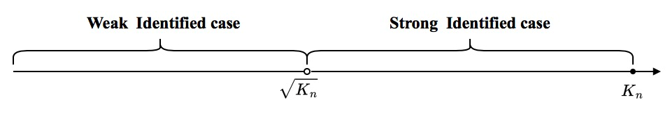
Figure 1: The strength of instruments when $K_{n}$ is large in terms of the order of $\mu_{n}^{2}$.

3 Unreliability of SY2005’s critical values

In this section, we first review SY2005’s influential procedure of obtaining critical values for detecting weak instruments. We then show the potential drawbacks of the critical values within the many instrument framework in two respects: when the number of instruments is large, 1) the classical $F$ test is oversized for detection of weak instruments; 2) the documented relationship between the relative bias and the concentration parameter breaks down.

3.1 SY2005’s procedure for fixed $K_{n}\equiv K$

We primarily focus on the 2SLS estimator and the single endogenous variable case for the sake of exposition clarity. SY2005 showed that the 2SLS estimator is inconsistent and the corresponding Wald test has incorrect size under their local-to-zero weak instrument asymptotics:

$$\pi=\frac{\mathbf{c}}{\sqrt{n}},$$ (4)

where $\mathbf{c}$ is a free vector. Building on these findings, while treating the number of instruments as a constant $K_{n}\equiv K$, Stock-Yogo introduced a definition of weak instruments based on either the magnitude of the 2SLS relative bias or the Wald test size distortion. Precisely, as a measure of the relative bias of 2SLS, they proposed the ratio

$$B_{n}^{2}=\frac{\mathrm{E}(\hat{\beta}^{2SLS}-\beta)^{\prime}{\Sigma}_{YY}\mathrm{E}(\hat{\beta}^{2SLS}-\beta)}{\mathrm{E}(\hat{\beta}^{OLS}-\beta)^{\prime}{\Sigma}_{YY}\mathrm{E}(\hat{\beta}^{OLS}-\beta)},$$ (5)

where $\Sigma_{YY}=\underset{n}{\mathrm{plim}}(\mathbf{Y}^{\prime}\mathbf{Y}/n)$. The instruments are deemed to be weak if the asymptotic relative bias is larger than a predetermined tolerance level. Under (4), they showed that

$$B_{n}\rightarrow B_{SY}=\left|\mathrm{E}\left[\frac{(\lambda+\xi)^{\prime}\xi}{(\lambda+\xi)^{\prime}(\lambda+\xi)}\right]\right|,$$ (6)

where $\lambda^{\prime}\lambda=\underset{n}{\lim}\mu_{n}^{2}$ and $\xi\sim N_{K}(\mathbf{0},\mathbf{I}_{K})$. It follows that the concentration parameter can fully characterize the asymptotic relative bias when the number of instruments is small. To test for weak instruments, they proposed the use of the first-stage $F$ statistic as it is connected with the relative bias via the concentration parameter. In fact, for testing the first-stage coefficient $\mathbf{\pi}$ is zero (the instruments are irrelevant), i.e. $H_{0}^{(1)}:\mathbf{\pi}=0$, it is well-known that under this null and as $n\rightarrow\infty$,

$$F=\frac{\mathbf{Y}^{\prime}\mathbf{P}_{Z}\mathbf{Y}/K}{\mathbf{Y}^{\prime}\mathbf{M}_{Z}\mathbf{Y}/(n-K)}\stackrel{{\scriptstyle d}}{{\rightarrow}}\frac{\chi^{2}_{K}}{K}.$$ (7)

It follows that $H_{0}^{(1)}$ is equivalent to $H_{0}^{(2)}:\mu_{n}^{2}=0$. When the instruments are irrelevant but weak, the concentration parameter is not exactly zero but close to it. Stock-Yogo then considered the testing problem: $H_{0}^{SY}:\mu_{n}^{2}\equiv\mu_{0}^{2}>0$. They showed that under (4),

$$F\stackrel{{\scriptstyle d}}{{\rightarrow}}\frac{\chi^{2}_{K}(\mu_{0}^{2})}{K},$$ (8)

where $\chi^{2}_{K}(\mu_{0}^{2})$ denotes the non-central Chi-squared distribution with $K$ degrees of freedom and noncentrality parameter $\mu_{0}^{2}$. Combining (6) with (8), Stock-Yogo proposed to calculate a critical value for $F$ as follows:

1. Choose a predetermined tolerance level $b$ for $B_{SY}$, for example, $b=0.1$.

2. Given $K$ and $b$, conduct simulation experiments to obtain $\lambda_{0}$ then $\mu_{0}^{2}$ by (6).

3. Determine a critical value for $F$ by (8).

The procedure above is summarized in Figure 2. Consequently, Stock-Yogo obtained a table of critical values for various combinations of $(p,K_{n},b)$, where $p$, $K_{n}$ and $b$ are up to 3, 30 and 0.3, respectively. Despite this effort, in empirical applications when $p=1$, researchers are more inclined to embrace the well-known “rule of thumb”: Reject the null of weak instruments when the first-stage $F$ statistic exceeds 10, corresponding to a relative bias of approximately 10% or less.

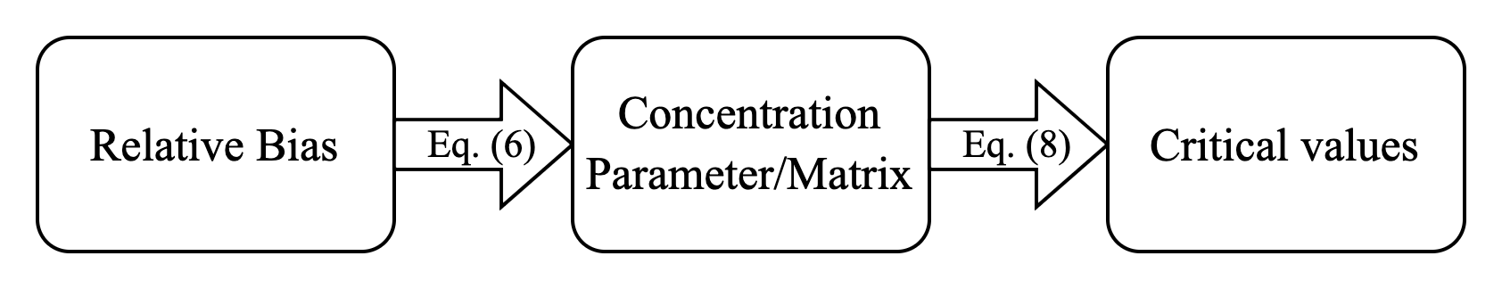
Figure 2: SY2005’s procedure for critical values of the first-stage $F$ statistic

3.2 Problems of SY2005’s critical values

For a fixed number of instruments, according to (8), the asymptotic expectation of $F$ is equivalent to $1+{\mu^{2}_{0}}/K_{n}$. Intuitively the first-stage $F$ statistic then can be less than 10 when $\mu_{0}^{2}/\sqrt{K_{n}}\rightarrow\infty$ but $\mu_{0}^{2}/K_{n}\rightarrow\kappa\in(0,\infty)$, that is, the instruments are strong and the first-stage $F$ test fails to detect this strength of instruments. Therefore, a low $F$ statistic does not necessarily mean that the identification and valid inference of $\beta$ is unachievable. In this sense, for large $K_{n}$, the classical first-stage $F$ statistic is not a good indicator of the weakness in instruments. This motivates us to study its performance with a large number of instruments.

3.2.1 Size distortions of the classical $F$ test

We first examine the empirical performance of the first-stage $F$ statistic using simulated experiments. Let $n=1000$ and consider $K_{n}=5,50$ and 500, for fixed number, moderate number, and large number of instruments, respectively. Consider further $\beta=1$, $\boldsymbol{Z}_{i}\stackrel{{\scriptstyle i.i.d.}}{{\sim}}N_{K_{n}}(\mathbf{0},\mathbf{I}_{K_{n}})$, and $(u_{i},v_{i})$ i.i.d. follows a centred bivariate normal with $\mathrm{E}(v_{i}^{2})=\mathrm{E}(u_{i}^{2})=1$ and $\mathrm{cov}(v_{i},u_{i})=0.9$. We set $\mathbf{\pi}=n^{-1/2}\boldsymbol{c}$ where $\boldsymbol{c}=\{c_{i}\}_{1\leq i\leq K_{n}}\stackrel{{\scriptstyle i.i.d.}}{{\sim}}N(0,\zeta^{2})$ with $\zeta$ carefully being such that the asymptotic relative bias can indicate the strength of instruments in the sense of SY2005’s definition. For example, we set $\zeta=1$ when $K_{n}=5$ so that the relative bias is within 10% tolerance level. The results from 10,000 independent replications are presented in Figure 1.

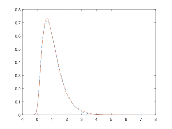
(a) $K_{n}=5$, $Avg.B_{n}^{2}=1.0$

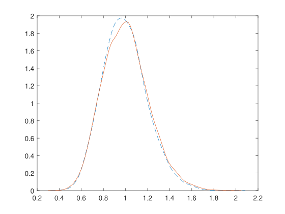
(b) $K_{n}=50$, $Avg.B_{n}^{2}=1.0$

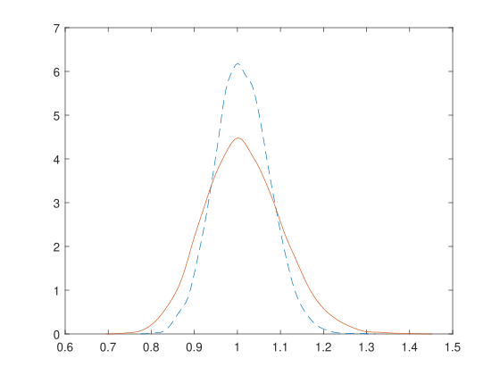
(c) $K_{n}=500$, $Avg.B_{n}^{2}=1.0$

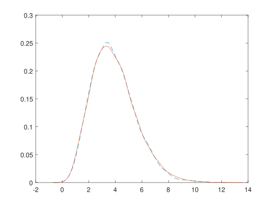
(d) $K_{n}=5$, $Avg.B_{n}^{2}=0.10$

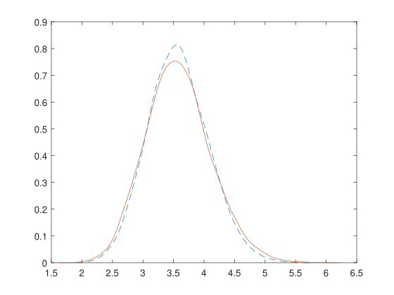
(e) $K_{n}=50$, $Avg.B_{n}^{2}=0.11$

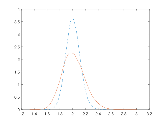
(f) $K_{n}=500$, $Avg.B_{n}^{2}=0.56$

Figure 3: The empirical density for the first-stage $F$ statistic (solid line) from 10,000 replications and the limiting noncentral Chi-squared distribution (dash line) predicted by SY2005 for various combinations of $(K_{n},B_{n}^{2})$. The sample size is $n=1000$.

The plots for both fixed and moderate $K_{n}$ manifest that the first-stage $F$ statistic is distributed close to the derived noncentral Chi-squared distribution. However, when the number of instruments is large ($K_{n}=500$), the distributions of $F$ fail to match its theoretical prediction, regardless of the strength of instruments. We then investigate the empirical sizes of SY2005’s procedure for $K_{n}=500$ and 800, again based on 10000 replications, and report the results in Table 1. We observe that the classical $F$ test is oversized for detecting weak instruments when the number of instruments is large. Applying Theorem 3 developed in Section 4, the following theorem confirmed this phenomenon.

Theorem 1.

(Size distortions of the classical $F$ test) When $\mu_{n}^{2}/K_{n}\rightarrow 0$, under Assumptions 1 and 2, as $n\rightarrow\infty$,

$$\mathbb{P}\left(F>\frac{q_{\tau}^{\chi^{2}_{K_{n}}(\mu_{0}^{2})}}{K_{n}}\right)\rightarrow\Phi\left(\sqrt{1-\alpha}\Phi^{-1}(\tau)\right)>\tau,$$

where $\tau$ is the significance level, $q_{\tau}^{\chi^{2}_{K_{n}}(\mu_{0}^{2})}$ is the $(1-\tau)$-quantile of $\chi^{2}_{K_{n}}(\mu_{0}^{2})$ distribution, and $\Phi^{-1}(\cdot)$ denotes the inverse cumulative distribution function of a standard normal random variable.

Theorem 1 shows that the classical $F$ test would be oversized as long as $\mu_{n}^{2}$ has the order smaller than $K_{n}$. The critical values reported by Stock-Yogo using the noncentral Chi-squared limiting distribution are therefore less trustworthy. As a numerical illustration, the predicted sizes in Theorem 1 are well confirmed by their empirical counterpart in the experiments, see the last column in Table 1.

	95% quantile of $F$	95% quantile of ${\frac{\chi^{2}_{K_{n}}(\mu_{0})}{K_{n}}}$	Empirical size	$\Phi\left(\sqrt{1-\frac{K_{n}}{n}}\Phi^{-1}(0.05)\right)$
$K_{n}=500$	1.17	1.12	12.6%	12.2%
$K_{n}=800$	1.23	1.10	23.0%	23.1%

Table 1: Empirical sizes and theoretical size in Theorem 1 of the first-stage $F$ test

3.2.2 Collapse of the relationship between $B_{n}^{2}$ and $\mu_{0}^{2}$

As presented in Figure 2, an essential step of Stock-Yogo’s procedure consists in establishing the relationship between the relative bias and the test statistics so that one can firstly obtain the noncentrality parameter according to (6), then the corresponding critical value as the limiting distribution of the test statistic is uniquely determined by the noncentrality parameter. In this section, we show that this relationship between the concentration parameter and the magnitude of the asymptotic relative bias no longer holds when the number of instruments is large. Consider the following linear IV model with multiple endogenous variables:

$$\underset{n\times 1}{\mathbf{y}}=\underset{n\times p}{\mathbf{Y}}\;\underset{p\times 1}{\boldsymbol{\beta}}+\underset{n\times 1}{\mathbf{u}},$$ (9)

$$\underset{n\times p}{\mathbf{Y}}=\underset{n\times K_{n}}{\mathbf{Z}}\underset{K_{n}\times p}{\boldsymbol{\Pi}}+\underset{n\times p}{\mathbf{V}},$$ (10)

where we still use $\mathbf{Y}$ for simplicity to denote the observations on the endogenous variables, and the $K_{n}\times p$ matrix $\boldsymbol{\Pi}$ is the first-stage coefficients. We assume the $(u_{i},\mathbf{V}_{i})^{\prime}$ are i.i.d. multivariate distributed with zero mean and $\mathrm{cov}(\mathbf{V}_{i})=\boldsymbol{\Sigma}_{VV}$, $\mathrm{var}(u_{i})=\sigma_{u}^{2}$ and $\mathrm{cov}(u_{i},\mathbf{V}_{i})=\boldsymbol{\Sigma}_{uV}$. The behavior of the 2SLS relative bias is characterized in the following theorem.

Theorem 2.

Under Assumptions 1 and 2, suppose that $\boldsymbol{\Pi}^{\prime}\mathbf{Z}^{\prime}\mathbf{Z}\boldsymbol{\Pi}/n\rightarrow\boldsymbol{\Theta}$ almost surely, as $n\rightarrow\infty$, we have almost surely,

$$B_{n}^{2}\rightarrow B^{2}=\frac{\alpha^{2}\boldsymbol{\Sigma}_{uV}\boldsymbol{\Theta}_{1}^{-1}\boldsymbol{\Theta}_{2}\boldsymbol{\Theta}_{1}^{-1}\boldsymbol{\Sigma}_{Vu}}{\boldsymbol{\Sigma}_{uV}\boldsymbol{\Theta}_{2}^{-1}\boldsymbol{\Sigma}_{Vu}},$$ (11)

where $\boldsymbol{\Theta}_{1}=\boldsymbol{\Theta}+\alpha\boldsymbol{\Sigma}_{VV}$ and $\boldsymbol{\Theta}_{2}=\boldsymbol{\Theta}+\boldsymbol{\Sigma}_{VV}$. In particular, if $\boldsymbol{\Theta}=0$, $B^{2}=1$, otherwise, $0<B^{2}<1$.

Theorem 2 shows that the relative bias will converge to a positive constant when the number of instrument is large. The limit is no more than one and it equals one only when the concentration parameter has the order smaller than $n$. Figure 4(a) shows the asymptotic relative bias $B_{SY}$ in (6) as a function of $\mu_{0}^{2}$ when $p=1$ and $K=5$, which is here continuous and decreasing in the concentration parameter. When the number of instruments is large, Figure 4(b) presents the asymptotic relative bias in (11) as a function of $\mu_{0}^{2}$, where the x-axis plots the order of $\mu_{0}^{2}$. Thus, the relationship between $B_{SY}$ and $\mu_{0}^{2}$ given in (6) for a small number of instruments no longer holds for the case of many instruments. Furthermore, as long as $\boldsymbol{\Pi}^{\prime}\mathbf{Z}^{\prime}\mathbf{Z}\boldsymbol{\Pi}/n\rightarrow 0$ (this scheme covers both the case of many weak instruments and the case of many strong instruments), the relative bias will converge to one. This finding indicates that testing for weak instruments based on the relative bias becomes conceptually unimplementable with a large number of instruments as 2SLS will always have the same level of bias as OLS does.

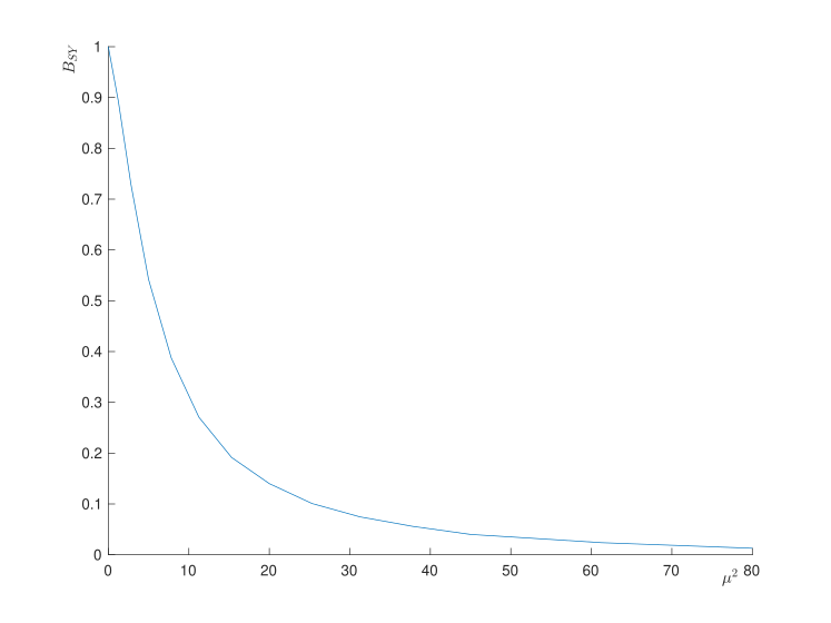
(a) $B_{SY}$ as a function of $\mu^{2}$ given in (6)

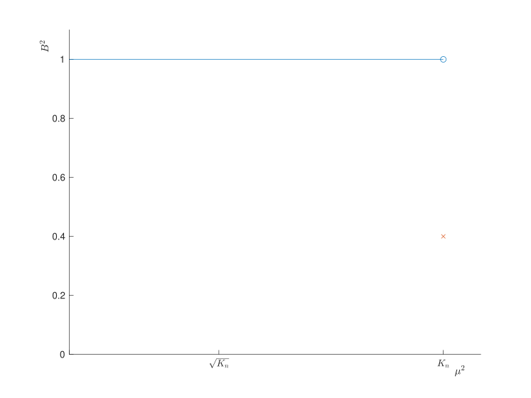
(b) $B^{2}$ as a function of $\mu^{2}$ given in (11)

Figure 4: The plotted relative bias as a function of the concentration parameter for the case of small number of instruments ($K_{n}=5$) and large number of instruments ($K_{n}=500$), respectively. The sample size is $n=1000$.

4 The first-stage $F$ statistic with many instruments

In this section, we first establish that when the number of instruments is large, the first-stage $F$ statistic is asymptotically normal after suitable normalization and recentering. We then apply the theory to assess the strength of many instruments by 1) constructing confidence intervals for ${\mu_{n}^{2}}/{\sqrt{K_{n}}}$; and 2) testing for many weak instruments.

Theorem 3.

When $\mu_{n}^{2}/K_{n}\rightarrow 0$ and under Assumptions 1 and 2, we have as $n\rightarrow\infty$,

$$\sqrt{n}(F-1-\frac{\mu_{n}^{2}}{K_{n}})\stackrel{{\scriptstyle d}}{{\rightarrow}}N\left(0,\frac{(\omega-\alpha^{2})\mathrm{E}(v_{1}^{4})+(2\alpha-3\omega+\alpha^{2})\sigma_{vv}^{4}}{\alpha^{2}(1-\alpha)^{2}\sigma_{vv}^{4}}\right),$$ (12)

where $\omega=\lim_{n\rightarrow\infty}\frac{1}{n}\sum_{i=1}^{n}P_{ii}^{2}$.

Note that we are particularly interested in the situation where $\mu_{n}^{2}$ grows no faster than $K_{n}$, which covers both the weakly identified and strongly identified cases. This asymptotic normality of $F$ is in sharp contrast with the limiting Chi-squared distributions in (7) and (8) established when the number of instruments is small. One may argue or guess the asymptotic normality from these Chi-squared distributions by allowing $K_{n}$, the degree of freedom, to increase to infinity. However, the precise renormalization and recenterning are nontrivial.

It is interesting at this point to compare Theorem 3 to Theorem 2 in Anatolyev (2012). For testing $H_{0}^{A}:\mu_{n}^{2}=0$, under an additional assumption that

$$P_{ii}\rightarrow\alpha,\;\text{uniformly in }i,$$ (13)

they showed that

$$\sqrt{n}(F-1)\stackrel{{\scriptstyle d}}{{\rightarrow}}N\left(0,\frac{2}{\alpha(1-\alpha)}\right).$$ (14)

Indeed, our asymptotic result in (12) reduces to (14) if $\mu_{n}^{2}=0$ and $P_{ii}\rightarrow\alpha$. Note that (13) is however restrictive as pointed out in Anatolyev (2012), Theorem 3 extends their result without this assumption while allowing for positive $\mu_{n}^{2}$. For further discussion, we consider the situation where the instruments are asymptotically balanced, a standard assumption considered by the literature (e.g., Hausman et al. 2012, Anatolyev and Gospodinov 2011 and Wang and Kaffo 2016), in the sense that

Assumption 3.

$n^{-1}\sum_{i=1}^{n}(P_{ii}-\alpha)^{2}\rightarrow 0$.

Note that Assumption 3 is weaker than (13). This assumption was discussed in details in Anatolyev and Yaskov (2017). Under this assumption, since $n^{-1}\sum_{i=1}^{n}P_{ii}=K_{n}/n\rightarrow\alpha$, we have $\omega=\alpha^{2}$ and the following result from Theorem 3.

Corollary 1.

When $\mu_{n}^{2}/K_{n}\rightarrow 0$, under Assumptions 1, 2 and 3, as $n\rightarrow\infty$,

$$\sqrt{n}(F-1-\frac{\mu_{n}^{2}}{K_{n}})\stackrel{{\scriptstyle d}}{{\rightarrow}}N\left(0,\frac{2}{\alpha(1-\alpha)}\right).$$ (15)

Therefore, compared to (14), the asymptotic variance of the first-stage $F$ statistic after correction remains the same but $\mu_{n}^{2}/K_{n}$ appears in the recentering term as long as $\mu_{n}^{2}$ is nonzero.

4.1 Confidence intervals for $\frac{\mu_{n}^{2}}{\sqrt{K_{n}}}$

When the number of weak instruments is small, the first-stage $F$ test statistic converges to a noncentral Chi-squared distribution given in (8). Ganics et al. (2021) suggested to construct confidence interval for the noncentrality parameter, $\mu_{0}^{2}$, based on the “symmetric range” confidence interval proposed in Kent and Hainsworth (1995). However, this method is generally not applicable for the case of a large number of instruments as the documented noncentral Chi-squared limiting distribution is not correct when the number of instruments is large, for example, in a comparable magnitude with the sample size.

Here based on Corollary 1, we can measure the strength of many instruments, ${\mu_{n}^{2}}/{\sqrt{K_{n}}}$, directly by constructing its ($1-\tau$) level asymptotic confidence interval as follows:

$$CI_{n}=\left[\sqrt{K_{n}}(F-1)-\sqrt{\frac{2n}{n-K_{n}}}\Phi^{-1}(1-\frac{\tau}{2}),\sqrt{K_{n}}(F-1)+\sqrt{\frac{2n}{n-K_{n}}}\Phi^{-1}(1-\frac{\tau}{2})\right].$$

This confidence interval method is beneficial in various ways. Firstly, the proposed confidence interval for the strength of many instruments can provide more information to applied researchers on quantifying the strength of instruments than the binary decision offered by tests. It can allow researchers to know how weak or strong their instruments are. Secondly, based on the corrected first-stage $F$ statistic, $CI_{n}$ is simple and computationally easy to calculate, as it is obtained from inverting asymptotic standard normal distribution. Also, constructing confidence intervals for $\mu_{n}^{2}/\sqrt{K_{n}}$ directly also avoids measuring its magnitude by solving complicated equations as in the SY2005’s procedure that requires the estimation bias or size distortions be equal to a predetermined tolerance level.

4.2 Testing for many weak instruments

In an elegant paper, MS2022 derived the asymptotic distribution of the JIVE-Wald test statistic and found its size distortion to be a function of

$$\tilde{\mu}_{n}^{2}=\Gamma^{-1/2}\pi^{\prime}\mathbf{Z}^{\prime}(\mathbf{P}_{Z}-\mathbf{D}_{Z})\mathbf{Z}\pi,$$

where $\Gamma$ is an unknown positive constant. To test for many weak instruments, they proposed a Jackknife-$F$ test statistic, $\widetilde{F}$, which asymptotically follows $N({\tilde{\mu}_{n}^{2}}/{\sqrt{K_{n}}},1)$ so that it depicts the strength of many instruments. They therefore apply $\widetilde{F}$ to detect many weak instruments by testing

$$H_{0}^{MS1}:\frac{\tilde{\mu}_{n}^{2}}{\sqrt{K_{n}}}\leq C_{0}.$$ (16)

Here the constant $C_{0}$ is obtained according to a predetermined tolerance level of the size of the JIVE-Wald test.

MS2022 showed that the two measures of the strength of instruments, $\mu_{n}^{2}$ and $\tilde{\mu}_{n}^{2}$, are of the same order if the $P_{ii}$’s are uniformly bounded. In fact, suppose that there exists a constant $\delta$ such that $P_{ii}\leq\delta<1$, we have

$$\frac{(1-\delta)\sigma_{vv}^{2}}{\sqrt{\Gamma}}\mu_{n}^{2}\leq\tilde{\mu}_{n}^{2}\leq\frac{\sigma_{vv}^{2}}{\sqrt{\Gamma}}\mu_{n}^{2}.$$ (17)

It is thus natural to consider the following null hypothesis

$$H_{0}:\frac{\mu_{n}^{2}}{\sqrt{K_{n}}}\leq C,$$ (18)

for some constant $C>0$ for the detection of many weak instruments.

Corollary 1 indicates that ${\mu_{n}^{2}}/{\sqrt{K_{n}}}$ appears in the recentering term if one multiply the factor $\sqrt{n}$ the recentering term $\mu_{n}^{2}/K_{n}$ together. It therefore enables ones to test for $H_{0}$ with the seminal first-stage $F$ test statistic when the number of instruments is large. To this end, we introduce the following corrected $F$ statistic for detecting many weak instruments by taking the equality in (18):

$$F_{c}=\sqrt{\frac{K_{n}(n-K_{n})}{2n}}\left[F-1-\frac{C}{\sqrt{K_{n}}}\right]$$ (19)

which is asymptotically standard normal under the equality in $H_{0}$ by Corollary 1. Therefore, a $\tau$ level test for $H_{0}$ is defined by the critical region $\{F_{c}>\Phi^{-1}(1-\tau)\}$.

4.2.1 The choice of $C$

According to SY2005 and MS2022, the instrument set is defined to be weak if $\mu_{n}^{2}$ (for a fixed number of instruments) or ${\mu_{n}^{2}}/{\sqrt{K_{n}}}$ (for many instruments) is bounded by an absolute constant. SY2005 and MS2022 obtain this constant by controlling the estimation bias or test distortions within a predetermined tolerance level. For the case of many instruments, MS2022 proposed $C_{0}$ in (16) to be 2.5 and thus suggested to reject $H_{0}^{MS}$ if $\widetilde{F}>4.14$ by controlling the size distortions of the Wald-JIVE test within 5% tolerance level of the nominal size. To implement the new $F_{c}$ test in (19), we need to determine the upper limit $C$ in (18). An ideal way would be to express the estimation bias or test distortions in terms of ${\mu_{n}^{2}}/{\sqrt{K_{n}}}$ based on the B2SLS estimator. However, it is challenging for multiple reasons. For example, we show that the asymptotic relative bias based on B2SLS has no explicit form when ${\mu_{n}^{2}}/{\sqrt{K_{n}}}$ is bounded in Appendix. This finding impedes determining the magnitude of $\mu_{n}^{2}$ given a tolerance level of estimation bias following the similar arguments in SY2005 and MS2022.

In this paper, we turn to make it straightforward and investigate the relationship between $C_{0}$ and $C$. According to (17), $H_{0}^{MS1}$ corresponds to testing

$$H_{0}^{MS2}:\frac{\mu_{n}^{2}}{\sqrt{K_{n}}}\leq\frac{C_{0}\sqrt{\Gamma}}{\sigma_{vv}^{2}}.$$ (20)

So it is natural to set $C={C_{0}\sqrt{\Gamma}}/{\sigma_{vv}^{2}}$. We then conduct Monte Carlo simulation experiments to examine the behavior of the factor ${\sqrt{\Gamma}}/{\sigma_{vv}^{2}}$ (the data generating process follows the same setting in Section 6.1.1). Table 2 shows that this factor is generally around 1, which indicates that $C$ and $C_{0}$ are comparable. We therefore propose $C\in[1,3]$ referring to the many weak instruments. Most of the simulation settings for weak instruments in literature corresponds to values of $C$ that are also consistent with the proposed range [1,3] (e.g. Wang and Zivot 1998, Hansen et al. 2008, Hausman et al. 2012 and Wang and Kaffo 2016).

Table 2: Empirical behaviors of ${\sqrt{\Gamma}}/{\sigma_{vv}^{2}}$ with $p=1$

$\mu_{n}^{2}/\sqrt{K_{n}}=1$ $\frac{K_{n}}{n}=\frac{1}{3}$ $\frac{K_{n}}{n}=\frac{1}{2}$ $\frac{K_{n}}{n}=\frac{2}{3}$ $K_{n}$ 50 100 200 300 500 50 100 200 300 500 50 100 200 300 500 ${\sqrt{\Gamma}}/{\sigma_{vv}^{2}}$ 1.01 1.25 1.13 1.11 1.19 0.79 1.16 0.96 0.93 1.02 0.38 0.86 0.76 0.77 0.82 $\mu_{n}^{2}/\sqrt{K_{n}}=2$ $\frac{K_{n}}{n}=\frac{1}{3}$ $\frac{K_{n}}{n}=\frac{1}{2}$ $\frac{K_{n}}{n}=\frac{2}{3}$ $K_{n}$ 50 100 200 300 500 50 100 200 300 500 50 100 200 300 500 ${\sqrt{\Gamma}}/{\sigma_{vv}^{2}}$ 1.01 1.25 1.13 1.11 1.19 0.80 1.16 0.96 0.93 1.02 0.38 0.85 0.76 0.77 0.82

4.2.2 Power of the $F_{c}$ test

Now we turn to investigate the power of the proposed $F_{c}$ test for testing instrument weakness. We consider the following two alternative hypotheses:

$$H_{A}^{(1)}:\frac{\mu_{n}^{2}}{\sqrt{K_{n}}}\rightarrow C_{A}\in(C,\infty),$$

$$H_{A}^{(2)}:\frac{\mu_{n}^{2}}{\sqrt{K_{n}}}\rightarrow\infty.$$

Theorem 4.

When $\mu_{n}^{2}/K_{n}\rightarrow 0$, under Assumptions 1, 2 and 3, as $n\rightarrow\infty$, we have

1. Under $H_{A}^{(1)}$,

   $$\mathbb{P}\left(F_{c}>\Phi^{-1}(1-\tau)\right)\rightarrow\Phi\left(\sqrt{\frac{2}{\alpha^{2}(1-\alpha)}}(C_{A}-C)-\Phi^{-1}(1-\tau)\right);$$ (21)

2. Under $H_{A}^{(2)}$,

   $$\mathbb{P}\left(F_{c}>\Phi^{-1}(1-\tau)\right)\rightarrow 1.$$ (22)

This theorem indicates that the proposed $F_{c}$ test has non-trivial asymptotic power as long as $\mu_{n}^{2}/K_{n}\rightarrow 0$. When $\mu_{n}^{2}/\sqrt{K_{n}}$ is bounded but greater than the cutoff $C$, the power of the corrected $F$ test depends on the distance $C_{A}-C$ and the ratio $\alpha$. When $\mu_{n}^{2}/\sqrt{K_{n}}$ is unbounded, $F_{c}$ turns to be consistent.

4.2.3 Comparison between $\widetilde{F}$ and $F_{c}$

As an ingenious test for many weak instruments, $\widetilde{F}$ is robust to heteroscedastic errors and allows for moderately many instruments (i.e., $K_{n}/n\rightarrow 0$). Compared to $\widetilde{F}$, our proposed $F_{c}$ test statistic is easy to implement, conceptually familiar and computationally simple. On the downside, it requires somewhat stringent assumptions. Besides, $F_{c}$ is valid as long as ${\mu_{n}^{2}}/{K_{n}}\rightarrow 0$. Whereas $\widetilde{F}$ requires ${\mu_{n}^{2}}/{K_{n}^{2/3}}\rightarrow 0$, which prevents researchers from assessing the strength of instruments when ${\mu_{n}^{2}}/{K_{n}^{2/3}}\rightarrow\infty$.

If empirical researchers are faced with many instruments and homoscedastic errors (Li and Yao 2019; Bai et al. 2018), we recommend applying our proposed $F_{c}$ test statistic to have a rapid and reliable assessment of the strength of instruments. Otherwise, the $\widetilde{F}$ test statistic should be used as it allows for the heteroscedastic errors and provides guidance to determine $C_{0}$ analytically.

5 Multiple endogenous variables

In this section, we first derive the limiting distribution of the trace of the Cragg-Donald statistic in the linear IV model with multiple endogenous variables defined in (9) and (10) within the many instrument setup. Based on this result, we propose explicit procedures for assessing the strength of many instruments with two endogenous variables.

For detection of weak instruments, Stock-Yogo proposed to use the minimum eigenvalue of the following Cragg-Donald statistic, which is the matrix analog of the first-stage $F$ statistic:

$$\mathbf{CD}=\frac{n-K_{n}}{K_{n}}(\mathbf{Y}^{\prime}\mathbf{M}_{Z}\mathbf{Y})^{-1}\mathbf{Y}^{\prime}\mathbf{P}_{Z}\mathbf{Y}.$$ (23)

The obtained test is documented to be conservative by applying a Chi-squared bound on the noncentral Wishart distribution. Stock-Yoho also found that the behavior of the test procedure depends on all eigenvalues of the Cragg-Donald statistic through the relative bias when the number of instruments increases. That is, when $p\geq 1$, the strength of instruments is contained in all eigenvalues of the concentration matrix $\boldsymbol{\Sigma}_{VV}^{-1/2}\boldsymbol{\Pi}^{\prime}\mathbf{Z}^{\prime}\mathbf{Z}\boldsymbol{\Pi}\boldsymbol{\Sigma}_{VV}^{-1/2}$. This finding motivates us to investigate the asymptotic behavior of the trace of (23) in case of many instruments. Let us define the strength of instruments with multiple endogenous variables as follows:

$$\theta_{n}^{2}={\mathrm{tr}(\boldsymbol{\Sigma}_{VV}^{-1/2}\boldsymbol{\Pi}^{\prime}\mathbf{Z}^{\prime}\mathbf{Z}\boldsymbol{\Pi}\boldsymbol{\Sigma}_{VV}^{-1/2})},$$

which reduces to $\mu_{n}^{2}$ when $p=1$. We then have the following result.

Theorem 5.

When $\theta_{n}^{2}/K_{n}\rightarrow 0$, under Assumptions 1 and 2, as $n\rightarrow\infty$, we have

$$\sqrt{n}\left(\mathrm{tr}(\mathbf{CD})-p-\frac{\theta_{n}^{2}}{K_{n}}\right)\stackrel{{\scriptstyle d}}{{\rightarrow}}N(0,\sigma_{0}^{2}),$$

where $\sigma_{0}^{2}=(1-\alpha)^{-2}\mathrm{vec}^{\prime}(\boldsymbol{\Sigma}_{VV}^{-1})\left(\alpha^{-2}\boldsymbol{\Sigma}_{4}-\boldsymbol{\Sigma}_{3}\right)\mathrm{vec}(\boldsymbol{\Sigma}_{VV}^{-1})$ with matrices $\boldsymbol{\Sigma}_{1}$ and $\boldsymbol{\Sigma}_{2}$ defined in (29) and (30) in Appendix, respectively.

Theorem 5 establishes the asymptotic distribution of the trace of the Cragg-Donald statistic under many instruments asymptotics: after suitable normalization and recentering, depending on the strength of instruments $\theta_{n}^{2}$, $\mathrm{tr}(\mathbf{CD})$ converges to a Gaussian variable. Note that this result holds for general number of endogenous variables and the errors can be nonnormal. Unfortunately, the limiting variance $\sigma_{0}^{2}$ has a complex form; it can be nonaccessible from data, see Remark 1. Hopefully, this problem vanishes for the case of two endogenous variables and we have the following result.

Corollary 2.

For $p=2$, when $\theta_{n}^{2}/K_{n}\rightarrow 0$, under Assumptions 1, 2 and 3, as $n\rightarrow\infty$,

$$\sqrt{n}\left(\mathrm{tr}(\mathbf{CD})-2-\frac{\theta_{n}^{2}}{K_{n}}\right)\stackrel{{\scriptstyle d}}{{\rightarrow}}N\left(0,\frac{4}{\alpha(1-\alpha)}\right).$$

Hence, when there are two endogenous variables, Corollary 2 allows us to construct confidence intervals for the strength of instruments and propose an additional test statistic for

$$H_{0}^{(2)}:\frac{\theta_{n}^{2}}{\sqrt{K_{n}}}\leq C$$ (24)

using the fact that

$$CD_{c}=\sqrt{\frac{K_{n}(n-K_{n})}{4n}}\left[\mathrm{tr}(\mathbf{CD})-2-\frac{C}{\sqrt{K_{n}}}\right],$$ (25)

is asymptotically standard normal under the equality in $H_{0}^{(2)}$.

Remark 1.

Obtaining the explicit form of $\sigma_{0}^{2}$ is tedious. For example, when $p=3$, if $\mathbf{v}_{i}\stackrel{{\scriptstyle i.i.d}}{{\sim}}N_{3}\left(\mathbf{0},\mathrm{diag}(\sigma_{1}^{2},\sigma_{2}^{2},\sigma_{3}^{2})\right)$, then the limiting variance is ${6}/\left({\alpha(1-\alpha)}\right)$ under the same assumptions. Generally, the limiting variance will depend on $\mathrm{E}(v_{i1}^{m_{1}}v_{i2}^{m_{2}}v_{i3}^{m_{3}})$ with non-negative integers $m_{1}$, $m_{2}$ and $m_{3}$ satisfying $m_{1}+m_{2}+m_{3}=4$ and the covariances between $v_{i1}$, $v_{i2}$ and $v_{i3}$.

6 Monte Carlo Simulations

The goal of this section is to evaluate the finite sample performance of the test procedure studied in the previous sections. In Section 6.1.1, we examine the empirical sizes and the empirical powers of $F_{c}$. Then the case of two endogenous variables is examined in Section 6.1.2. Section 6.2 reports the simulation results.

6.1 Monte Carlo designs

6.1.1 The single endogenous variable case

We consider the following first-stage setup

$$Y_{i}=\pi^{\prime}\mathbf{Z}_{i}+v_{i},$$

where $\boldsymbol{Z}_{i}\stackrel{{\scriptstyle i.i.d.}}{{\sim}}N_{K_{n}}(\mathbf{0},\mathbf{I}_{K_{n}})$, for $i=1,\dots,n$. The number of instruments $K_{n}$ varies in $\{50,100,200,500,1000\}$ with corresponding sample sizes satisfying three different ratios ${K_{n}}/{n}={1}/{3},{1}/{2}$ and ${2}/{3}$, respectively. For the error terms, we generate them from two distributions: (i) standard normal $N(0,1)$, and (ii) Chi-squared $(\chi_{2}^{2}-2)/2$. To generate data under the null, we specify $C\in\{1,2\}$ and set $\mathbf{\pi}=c_{n}n^{-1/2}\mathbf{c}$ with $\mathbf{c}=(1,\dots,1)^{\prime}$ being a $K_{n}\times 1$ vector. The scale $c_{n}$ is carefully chosen such that ${\mu_{n}^{2}}/{\sqrt{K_{n}}}=C$. For example, we set $c_{n}=0.215$ so that ${\mu_{n}^{2}}/{\sqrt{K_{n}}}=1$ for $(K_{n},n)=(500,1500)$. To examine the empirical powers, we consider testing $H_{0}:{\mu_{n}^{2}}/{\sqrt{K_{n}}}\leq 1$ and generate the data subjected to $C\in\{2,3,4,5,6,7,8,9,10,11\}$ for $K_{n}=500$ with normal errors. The Monte Carlo experiments are conducted with 2000 replications.

6.1.2 The two endogenous variables case

We specify the DGP for the first-stage model as following:

$$\mathbf{Y}_{i}=\boldsymbol{\Pi}^{\prime}\mathbf{Z}_{i}+\mathbf{V}_{i},$$

where $\boldsymbol{Z}_{i}$, $K_{n}$, and $n$ are generated in the same way as in the single endogenous variable case. We generate the errors terms according to bivariate normal distribution with zero mean and covariance matrix, $\left((2,3)^{\prime},(3,6)^{\prime}\right)$. The DGP for the null is similar to the one in the single endogenous variable case, where we set $\theta_{n}^{2}/{\sqrt{K_{n}}}\in\{1,2\}$. We also examine the empirical powers for testing $\theta_{n}^{2}/{\sqrt{K_{n}}}\leq 1$ when the data are generated such that $\theta_{n}^{2}/{\sqrt{K_{n}}}$ ranges in $\{2,3,4,5,6,7,8,9,10,11\}$ for $K_{n}=500$ with normal errors. The Monte Carlo experiments again use 2000 replications.

6.2 Simulation results

For $p=1$, the upper panel and the lower panel of Table 3 report the empirical sizes of the $F_{c}$ test with 5% and 10% nominal sizes for testing ${\mu_{n}^{2}}/\sqrt{K_{n}}\leq 1$ and ${\mu_{n}^{2}}/\sqrt{K_{n}}\leq 2$, respectively. It is evident that our proposed $F_{c}$ test produces empirical sizes around the nominal values when both $K_{n}$ and $n$ are large, irrespective of the error distributions. Some incremental size distortions can be detected when both $K_{n}$ and $n$ are small and as $C$ rises. For example, the empirical size rises from 6.75% to 8.85% when ${K_{n}}/{n}={1}/{3}$ with $K_{n}=200$ and when $C$ rises from 1 to 2 under normal errors. The proposed test is also oversized when $K_{n}$ is small, e.g., the empirical size is 11.9% when $C=2$, $K_{n}=50$ with ${K_{n}}/{n}={1}/{3}$, normal errors and 5% nominal size. These anomalies are expected when $K_{n}$ and $n$ take small values since our results apply to high dimensional framework, but they disappear as $n$ increases. For fixed ratio $n/T$, the empirical sizes converge to the nominal sizes as $n\rightarrow\infty$, which authenticates the asymptotic normality of the tests under the many instruments asymptotics. For $p=2$, Table 4 demonstrates the empirical sizes of the $CD_{c}$ test with 5% and 10% nominal sizes for testing ${\mu_{n}^{2}}/\sqrt{K_{n}}\leq 1$ and ${\mu_{n}^{2}}/\sqrt{K_{n}}\leq 2$, respectively. The findings are similar to the case of $p=1$, which show that the proposed test can generally control sizes well.

Next, we turn to Figure 5 and 6 which show the empirical powers for testing ${\mu_{n}^{2}}/\sqrt{K_{n}}\leq 1$ of $F_{c}$ and $CD_{c}$, respectively. When the departure from the null is small, the two tests does not produce very high empirical power, which is indicated by (21). As the alternative hypothesis becomes more distant the empirical power rises, e.g., the empirical power of the $F_{c}$ test increases to 98.55% with ${K_{n}}/{n}={1}/{3}$ under $H_{1}:{\mu_{n}^{2}}/\sqrt{K_{n}}=9$, which is also shown in (22). The empirical powers of the $CD_{c}$ test also present a similar finding.

Table 3: Empirical sizes with $p=1$ for the nominal values at 5% and 10%

$C=1$ $\frac{K_{n}}{n}=\frac{1}{3}$ $\frac{K_{n}}{n}=\frac{1}{2}$ $\frac{K_{n}}{n}=\frac{2}{3}$ $K_{n}=$ 50 100 200 300 500 50 100 200 300 500 50 100 200 300 500 Normal 5% 8.1 6.95 6.75 5.6 5.5 7.85 8.45 7.1 7.1 5.55 11.25 8.55 6.9 6.2 4.95 10% 14.5 11.55 12.15 11.1 11.3 13.65 14.95 13.05 12.3 10 16.2 13.5 13.15 12.25 10.5 Chi squared 5% 8.1 8.05 7.25 5.7 6.05 10.25 7.1 7.5 5.6 5.75 11.3 9.35 7.3 6.85 5.6 10% 13.95 14.2 12.6 10 11.7 15.6 12.85 12.55 10.45 10.95 16.1 14.3 12.05 11.8 9.85 $C=2$ $\frac{K_{n}}{n}=\frac{1}{3}$ $\frac{K_{n}}{n}=\frac{1}{2}$ $\frac{K_{n}}{n}=\frac{2}{3}$ $K_{n}=$ 50 100 200 300 500 50 100 200 300 500 50 100 200 300 500 Normal 5% 11.9 8.9 8.85 6.75 6.15 11.5 11.2 8.65 8.3 6 14.2 10.35 8.8 7.55 5.6 10% 18.5 15.6 14.55 12.05 12.4 17.65 17.75 15.3 13.6 11.11 20.1 16.9 15.25 13.7 11.55 Chi squared 5% 12.1 11.45 8.9 6.45 7.05 14.4 10.2 8.6 6.75 6.25 14.9 11.5 9.3 7.8 6.05 10% 18.05 18 15.85 11.45 12.25 20.65 16.65 15.15 12.25 11.8 21.15 18.1 15.05 13.55 11.2

Table 4: Empirical sizes with $p=2$ and normal errors for nominal levels at 5% and 10%

$C=1$ $\frac{K_{n}}{n}=\frac{1}{3}$ $\frac{K_{n}}{n}=\frac{1}{2}$ $\frac{K_{n}}{n}=\frac{2}{3}$ $K_{n}=$ 50 100 200 300 500 50 100 200 300 500 50 100 200 300 500 Normal 5% 8.4 6.65 6.4 6.05 5.8 9.95 8.3 7.7 6.95 5.95 15.45 10.35 7.9 6.5 5.2 10% 15.45 11.55 11.8 11.65 10.9 15 13.4 13.4 11.75 10.7 20.95 16.3 13.3 11.5 9.95 $C=2$ $\frac{K_{n}}{n}=\frac{1}{3}$ $\frac{K_{n}}{n}=\frac{1}{2}$ $\frac{K_{n}}{n}=\frac{2}{3}$ $K_{n}=$ 50 100 200 300 500 50 100 200 300 500 50 100 200 300 500 Normal 5% 10.35 7.7 7.15 6.75 5.8 11.95 9.6 8.7 7.4 6.65 16.65 11.3 8.6 7.15 5.55 10% 16.5 13.45 12.9 12.35 11.85 18 15.65 14.4 12.45 11.2 23.25 18.15 14.45 12.3 10.5

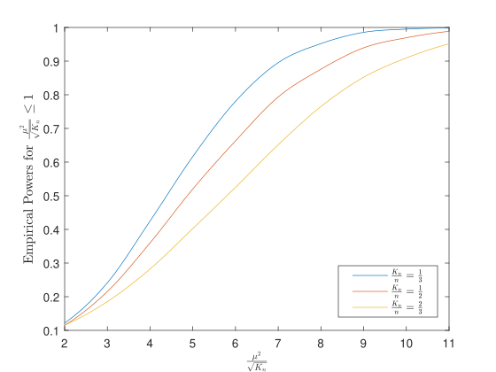
Figure 5: Empirical powers of $F_{c}$

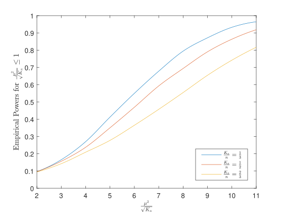
Figure 6: Empirical powers of $CD_{c}$

7 An empirical illustration: Return to education

In this section, we re-analyse the returns to education data of Angrist and Keueger (1991) (henceforth referred to as AK1991) using quarter of birth as an instrument for educational attainment, and construct confidence intervals for the strength of instruments. One of the specifications in the original AK1991 application uses up to 180 instruments that include 30 quarter and year of birth interactions and 150 quarter and state of birth interactions. At the time of publication, the issue of weak instruments had received little attention. Later it has been widely suggested that the setup suffers from a weak instrument problem (Angrist and Krueger 1995; Bound et al. 1995). MS2022 applied their proposed pre-test and argued the instrument set is strong with the original full data.

As their original sample size (329,509) is larger than usual for empirical research, we consider the sample size to be 0.1%($n=330$), 0.2%($n=660$), 0.5%($n=1650$) and 1%($n=3300$) of the original sample size, more in line with the typical empirical application. We examine the specification with 180 instruments and 1350 instruments that extend the model by including the interactions among quarter and year and state of birth. We evaluate the performance of the first-stage $F$ statistic, the $\widetilde{F}$ statistic based confidence intervals and our proposed confidence intervals based on 2000 randomly chosen subsamples and report the results in Table 5.

For the 0.1% subsample with 180 instruments, the average $F$ statistics is 1.53, which is far below the classical cut-off of 10. However, the confidence interval for ${\tilde{\mu}_{n}^{2}}/({\sqrt{K_{n}}\sqrt{\Gamma}})$ based on $\widetilde{F}$ is [3.15,6.43], which does not cover the cutoff of 2.5 suggested by MS2022. It provides an evidence that 0.1%-scheme produces strong instruments subsamples. Our proposed confidence interval for ${\mu_{n}^{2}}/{\sqrt{K_{n}}}$ turns out to be [3.67,10.55], which also claims that the instrument set is strong. When the sample size increases to 660, the first-stage $F$ statistic is uninformative. While both our proposed confidence interval and the $\widetilde{F}$ based confidence interval determine the instruments to be weak. The findings for the case of 1350 instruments are similar.

We also observe that our proposed confidence intervals are close to the $\widetilde{F}$ based ones, which is consistent with the argument in previous section. Though inherently wider compared to those obtained from $\widetilde{F}$, our proposed confidence intervals are still informative to identify the strength of instruments.

$n$	$K_{n}$	Avg.$F$	$\tilde{F}$-95% CIs	The proposed 95% CIs
330	180	1.53	[3.15,6.43]	[3.67,10.55]
660	180	1.06	(0,3.2]	(0,3.5]
1650	1350	1.26	[2.81,6.09]	[4.14,14.51]
3300	1350	1.06	(0,2.76]	(0,5.24]

Table 5: Empirical Results

8 Conclusion

Empirical researchers often embrace a large number of instruments which are potentially weak. To detect weak instruments, we show that the classical first-stage $F$ test tends to over-reject for IV models with many instruments. We derive the asymptotic distribution of a corrected $F$ statistic and propose a valid test for weak instruments when there are many instruments. The proposed corrected first-stage $F$ statistic is easy to implement, conceptually familiar and computationally simple. The test statistic can also be applied to construct confidence intervals for the concentration parameter, allowing researchers to determine the strength of instruments.

For the case of multiple endogenous variables, we derive the asymptotic distribution of the trace of the Cragg-Donald statistic, which contains the information of all eigenvalues of the concentration matrix, and propose a test for weak instruments in IV models for the case of two endogenous variables. The test statistic also enables researchers to determine the strength of identification when there are many instruments.

A limitation of our test statistic is the assumption that the errors are homoscedastic. Theoretical extensions that deal with heteroscedasticity and serial correlation are interesting avenues for future research.

Appendix A Proofs of main results

We first prove Theorem 3, then prove Theorem 1 and 4 applying Theorem 3. Then we prove Theorem 2. Finally, the proof of Theorem 5 is completed by applying the central limit theorem of sesquilinear forms proposed in Wang et al. (2014).

A.1 Proof of Theorem 3

Denote $\boldsymbol{\Upsilon}=\mathbf{Z}\pi$, we first establish the following lemma:

Lemma 1.

Under Assumptions 1 and 2, as $n\rightarrow\infty$,

$$\left(\frac{\mathbf{v}^{\prime}\mathbf{v}-n\sigma_{vv}^{2}}{\sqrt{n}},\frac{\mathbf{v}^{\prime}\mathbf{P}_{Z}\mathbf{v}-K_{n}\sigma_{vv}^{2}}{\sqrt{n}}\right)^{\prime}\stackrel{{\scriptstyle d}}{{\rightarrow}}N\left(\mathbf{0},(\boldsymbol{\Sigma}_{ij})_{i,j=1,2}\right),$$

with

$$\boldsymbol{\Sigma}_{11}=\mathrm{Var}(v_{1}^{2}),\;\boldsymbol{\Sigma}_{22}=\omega\mathrm{E}(v_{1}^{4})+(2\alpha-3\omega)\sigma_{vv}^{4},\;and\;\boldsymbol{\Sigma}_{12}=\alpha\mathrm{Var}(v_{1}^{2}).$$

Proof.

We apply Theorem 2 in Wang et al. (2014) by setting $\mathbf{A}_{n}=\mathbf{I}_{n}$ and $\mathbf{B}_{n}=\mathbf{P}_{Z}$. We verify that their defined quantities $\omega_{1}=\theta_{1}=\tau_{1}=1$, $\theta_{2}=\tau_{2}=\omega_{3}=\theta_{3}=\tau_{3}=\alpha$ and $\omega_{2}=\omega$ exists since the leverage value $P_{ii}$ ranges in $[0,1]$. One can verify $A_{1}=\mathrm{Var}(v_{1}^{2})$, $A_{2}=A_{3}=\sigma_{vv}^{4}$ in Theorem 2 of Wang et al. (2014), which completes the proof. ∎

To prove Theorem 3, firstly note that

$$F=\frac{n-K_{n}}{K_{n}}\frac{\frac{\boldsymbol{\Upsilon}^{\prime}\boldsymbol{\Upsilon}}{n}+2\frac{\mathbf{v}^{\prime}\boldsymbol{\Upsilon}}{n}+\frac{\mathbf{v}^{\prime}\mathbf{P}_{Z}\mathbf{v}}{n}}{\frac{\mathbf{v}^{\prime}\mathbf{v}}{n}-\frac{\mathbf{v}^{\prime}\mathbf{P}_{Z}\mathbf{v}}{n}}.$$

Besides,

$$\frac{\mathbf{v}^{\prime}\boldsymbol{\Upsilon}}{n}=o_{p}(\frac{1}{\sqrt{n}})$$

as

$$\mathrm{E}\left(\frac{\mathbf{v}^{\prime}\boldsymbol{\Upsilon}}{n}\right)^{2}=\mathrm{E}\left(\frac{\boldsymbol{\Upsilon}^{\prime}\mathbf{v}\mathbf{v}^{\prime}\boldsymbol{\Upsilon}}{n^{2}}\right)=\sigma_{vv}^{2}\frac{\boldsymbol{\Upsilon}^{\prime}\boldsymbol{\Upsilon}}{n^{2}}=o(\frac{1}{n}).$$

We then can apply Delta method with Lemma 1 and the function $f:\mathbb{R}^{2}\rightarrow\mathbb{R}$ satisfying that

$$f\left(\frac{\mathbf{v}^{\prime}\mathbf{v}}{n},\frac{\mathbf{v}^{\prime}\mathbf{P}_{Z}\mathbf{v}}{n}\right)=F.$$

We have

$$\nabla f\left(\sigma_{vv}^{2},\frac{K_{n}}{n}\sigma_{vv}^{2}\right)=\left(-\frac{n\sum_{i=1}\Upsilon_{i}^{2}+nK_{n}\sigma_{vv}^{2}}{K_{n}(n-K_{n})\sigma_{vv}^{4}},\frac{n\sum_{i=1}\Upsilon_{i}^{2}+n^{2}\sigma_{vv}^{2}}{K_{n}(n-K_{n})\sigma_{vv}^{4}}\right),$$

which yields with Lemma 1 that

$$\sqrt{n}(F-1-\frac{\mu_{n}^{2}}{K_{n}})\stackrel{{\scriptstyle d}}{{\rightarrow}}N\left(0,\frac{(\omega-\alpha^{2})\mathrm{E}(v_{1}^{4})+(2\alpha-3\omega+\alpha^{2})\sigma_{vv}^{4}}{\alpha^{2}(1-\alpha)^{2}\sigma_{vv}^{4}}\right).$$

A.2 Proof of Theorem 1

By the noncentral Chi-squared distribution’s normal approximation for large $K_{n}$, we verify that

$$q_{\tau}^{\chi^{2}_{K_{n}}(\mu_{0}^{2})}=\frac{K_{n}+\mu_{0}^{2}}{2K_{n}+4\mu_{0}^{2}}\left(\Phi^{-1}(1-\tau)+\sqrt{2K_{n}+4\mu_{0}^{2}}\right)^{2}+O(1),$$

so

$$\frac{q_{\tau}^{\chi^{2}_{K_{n}}(\mu_{0}^{2})}}{K_{n}}-1=\frac{1+\mu_{0}^{2}/{K_{n}}}{2K_{n}+4\mu_{0}^{2}}(\Phi^{-1}(1-\tau))^{2}+\frac{2+2\mu_{0}^{2}/K_{n}}{\sqrt{2K_{n}+4\mu_{0}^{2}}}\Phi^{-1}(1-\tau)+\frac{\mu_{0}^{2}}{K_{n}}+O(\frac{1}{K_{n}}).$$

Then, using Theorem 3,

$$\mathbb{P}\left(K_{n}F>q_{\tau}^{\chi^{2}_{K_{n}}(\mu_{0}^{2})}\right) =\mathbb{P}\left(\sqrt{\frac{\alpha(1-\alpha)}{2}}\sqrt{n}(F-1-\frac{\mu_{0}^{2}}{K_{n}})>\sqrt{\frac{\alpha(1-\alpha)}{2}}\sqrt{n}(\frac{q_{\tau}^{\chi^{2}_{K_{n}}(\mu_{0}^{2})}}{K_{n}}-1-\frac{\mu_{0}^{2}}{K_{n}})\right)$$

$$=\mathbb{P}\left(\sqrt{\frac{\alpha(1-\alpha)}{2}}\sqrt{n}(F-1-\frac{\mu_{0}^{2}}{K_{n}})>\sqrt{\frac{\alpha(1-\alpha)}{\alpha+2\mu_{0}^{2}/n}}\Phi^{-1}(1-\tau)+o(1)\right)$$

$$\rightarrow 1-\Phi\left(\sqrt{1-\alpha}\Phi^{-1}(1-\tau)\right)>\tau.$$

A.3 Proof of Theorem 4

Denote $\hat{\sigma}_{0}={(K_{n}(n-K_{n}))}/{2n^{2}}$ be the estimator of the limiting variance of $(\alpha(1-\alpha))/2$ in (15). For the $F_{c}$ test, we have

$$\mathbb{P}\left(F_{c}>\Phi^{-1}(1-\tau)\right)=\mathbb{P}\left(\hat{\sigma}_{0}^{-1}\sqrt{n}(F-1-\frac{\mu_{n}^{2}}{K_{n}})+\underbrace{\hat{\sigma}_{0}^{-1}\sqrt{\frac{n}{K_{n}}}(\frac{\mu_{n}^{2}}{\sqrt{K_{n}}}-C)}_{\delta_{0}}>\Phi^{-1}(1-\tau)\right).$$

Under $H_{A}^{(1)}$, note that $\delta_{0}\rightarrow\sqrt{\frac{2}{\alpha^{2}(1-\alpha)}}(C_{A}-C)$, we have

$$\mathbb{P}\left(F_{c}>\Phi^{-1}(1-\tau)\right)\rightarrow 1-\Phi\left(\Phi^{-1}(1-\tau)-\sqrt{\frac{2}{\alpha^{2}(1-\alpha)}}(C_{A}-C)\right).$$

Under $H_{A}^{(2)}$, note that $\delta_{0}\rightarrow\infty$, so that

$$\mathbb{P}\left(F_{c}>\Phi^{-1}(1-\tau)\right)\rightarrow 1.$$

Now we complete the proof of Theorem 4.

A.4 Proof of Theorem 2

We first introduce the following lemma which establishes the probabilistic limit of 2SLS and OLS within the many instruments setup.

Lemma 2.

(Theorem 1, Huang et al. 2022) Under Assumptions 1 and 2, as $n\rightarrow\infty$, (a) when $\boldsymbol{\Pi}^{\prime}\mathbf{Z}^{\prime}\mathbf{Z}\boldsymbol{\Pi}/n\rightarrow\boldsymbol{\Theta}$ almost surely, $\hat{\boldsymbol{\beta}}^{2SLS}\stackrel{{\scriptstyle p}}{{\rightarrow}}\boldsymbol{\beta}+\alpha\boldsymbol{\Theta}_{1}^{-1}\boldsymbol{\Sigma}_{Vu}$, $\hat{\boldsymbol{\beta}}^{OLS}\stackrel{{\scriptstyle p}}{{\rightarrow}}\boldsymbol{\beta}+\boldsymbol{\Theta}_{2}^{-1}\boldsymbol{\Sigma}_{Vu}$; (b) when $\boldsymbol{\Pi}^{\prime}\mathbf{Z}^{\prime}\mathbf{Z}\boldsymbol{\Pi}/n\rightarrow\boldsymbol{0}$ almost surely, both $\hat{\boldsymbol{\beta}}^{2SLS}$ and $\hat{\boldsymbol{\beta}}^{OLS}$ converge in probability to $\boldsymbol{\beta}+\boldsymbol{\Sigma}_{VV}^{-1}\boldsymbol{\Sigma}_{Vu}$.

To prove Theorem 2, we observe that results of convergence of $B_{n}^{2}$ holds naturally by applying Theorem 2 directly. Now, we show that $B^{2}<1$ when $\boldsymbol{\Pi}^{\prime}\mathbf{Z}^{\prime}\mathbf{Z}\boldsymbol{\Pi}/n\rightarrow\boldsymbol{0}$. Define the degrees of simultaneity $\boldsymbol{\rho}=\boldsymbol{\Theta}_{2}^{-1/2}\boldsymbol{\Sigma}_{Vu}$, then

$$B^{2}=\frac{\alpha^{2}\boldsymbol{\rho}^{\prime}\boldsymbol{\Theta}_{2}^{1/2}\boldsymbol{\Theta}_{1}^{-1}\boldsymbol{\Theta}_{2}\boldsymbol{\Theta}_{1}^{-1}\boldsymbol{\Theta}_{2}^{1/2}\boldsymbol{\rho}}{\boldsymbol{\rho}^{\prime}\boldsymbol{\rho}}.$$

Similar to Stock and Yogo (2005), we consider the worst-case asymptotic relative bias

$$B_{\max}^{2}=\max_{\boldsymbol{\rho}}|B|^{2}.$$

It can be shown that $B_{\max}^{2}=\lambda_{1}(\alpha^{2}\boldsymbol{\Theta}_{2}^{1/2}\boldsymbol{\Theta}_{1}^{-1}\boldsymbol{\Theta}_{2}\boldsymbol{\Theta}_{1}^{-1}\boldsymbol{\Theta}_{2}^{1/2})$. Note that $\boldsymbol{\Theta}_{1}/\alpha-\boldsymbol{\Theta}_{2}=(1-\alpha)/\alpha\boldsymbol{\Theta}$ is positive definite, we have

$$\alpha\boldsymbol{\Theta}_{2}^{1/2}\boldsymbol{\Theta}_{1}^{-1}\boldsymbol{\Theta}_{2}^{1/2} =\boldsymbol{\Theta}_{2}^{1/2}(\frac{1-\alpha}{\alpha}\boldsymbol{\Theta}+\boldsymbol{\Theta}_{2})^{-1}\boldsymbol{\Theta}_{2}^{1/2}$$

$$=\boldsymbol{\Theta}_{2}^{1/2}\left(\boldsymbol{\Theta}_{2}^{-1}-\boldsymbol{\Theta}_{2}^{-1}(\boldsymbol{\Theta}_{2}^{-1}+\frac{\alpha}{1-\alpha}\boldsymbol{\Theta}^{-1})^{-1}\boldsymbol{\Theta}_{2}^{-1}\right)\boldsymbol{\Theta}_{2}^{1/2}$$

$$=\mathrm{I}_{p}-\boldsymbol{\Theta}_{2}^{-1/2}(\boldsymbol{\Theta}_{2}^{-1}+\frac{\alpha}{1-\alpha}\boldsymbol{\Theta}^{-1})^{-1}\boldsymbol{\Theta}_{2}^{-1/2},$$ (26)

where the second equality follows from the Woodbury matrix identity. Next, by Weyl’s inequality, it follows that

$$\lambda_{1}(\alpha\boldsymbol{\Theta}_{2}^{1/2}\boldsymbol{\Theta}_{1}^{-1}\boldsymbol{\Theta}_{2}^{1/2})+\lambda_{p}\left(\boldsymbol{\Theta}_{2}^{-1/2}(\boldsymbol{\Theta}_{2}^{-1}+\frac{\alpha}{1-\alpha}\boldsymbol{\Theta}^{-1})^{-1}\boldsymbol{\Theta}_{2}^{-1/2}\right)\leq 1.$$

Note that $\boldsymbol{\Theta}_{2}^{-\frac{1}{2}}(\boldsymbol{\Theta}_{2}^{-1}+\frac{\alpha}{1-\alpha}\boldsymbol{\Theta}^{-1})^{-1}\boldsymbol{\Theta}_{2}^{-\frac{1}{2}}$ is positive definite, then $\lambda_{1}(\alpha^{2}\boldsymbol{\Theta}_{2}^{1/2}\boldsymbol{\Theta}_{1}^{-1}\boldsymbol{\Theta}_{2}\boldsymbol{\Theta}_{1}^{-1}\boldsymbol{\Theta}_{2}^{1/2})\leq\lambda_{1}^{2}(\alpha\boldsymbol{\Theta}_{2}^{1/2}\boldsymbol{\Theta}_{1}^{-1}\boldsymbol{\Theta}_{2}^{1/2})<1$.

A.5 Proof of Theorem 5

To prove Theorem 5, we introduce Lemma 3, which establishes the joint CLT of four sesquilinear forms that make up the Cragg-Donald statistic, and then apply Delta method to it.

We firstly define the following variables:

$$\dot{\mathbf{V}}:=\left[\underbrace{\overbrace{\mathbf{V}(1),\cdots,\mathbf{V}(1)}^{p},\cdots,\overbrace{\mathbf{V}(p),\cdots,\mathbf{V}(p)}^{p}}_{p^{2}}\right]\in\mathbb{R}^{n\times p^{2}},$$ (27)

and

$$\ddot{\mathbf{V}}:=\left[\underbrace{\overbrace{\mathbf{V}(1),\cdots,\mathbf{V}(p)}^{p},\cdots,\overbrace{\mathbf{V}(1),\cdots,\mathbf{V}(p)}^{p}}_{p^{2}}\right]\in\mathbb{R}^{n\times p^{2}}.$$ (28)

We then establish the joint distribution of two key components which make up the Cragg-Donald statistic in the following lemma:

Lemma 3.

Under Assumption 1 and 2, as $n\rightarrow\infty$, we have

$$\sqrt{n}\cdot\left[\left(\begin{array}[]{l}n^{-1}\mathrm{vec}(\mathbf{V}^{\prime}\mathbf{V})\\ n^{-1}\mathrm{vec}(\mathbf{V}^{\prime}\mathbf{P}_{Z}\mathbf{V})\end{array}\right)-\left(\begin{array}[]{c}\mathrm{vec}(\boldsymbol{\Sigma}_{VV})\\ \frac{K_{n}}{n}\mathrm{vec}(\boldsymbol{\Sigma}_{VV})\end{array}\right)\right]\stackrel{{\scriptstyle d}}{{\rightarrow}}N\left(\mathbf{0},\boldsymbol{\Sigma}_{0}\right),$$

where

$$\boldsymbol{\Sigma}_{0}=\left[\begin{array}[]{cc}\boldsymbol{\Sigma}_{1}&\alpha\boldsymbol{\Sigma}_{1}\\ \alpha\boldsymbol{\Sigma}_{1}&\boldsymbol{\Sigma}_{2}\end{array}\right]$$

with

$$\boldsymbol{\Sigma}_{1,ij}=\mathrm{Cov}(\dot{V}_{1i}\ddot{V}_{1i},\dot{V}_{1j}\ddot{V}_{1j}),$$ (29)

$$\boldsymbol{\Sigma}_{2,ij}=\omega\boldsymbol{\Sigma}_{11,ij}+(\alpha-\omega)\left(\mathrm{E}(\dot{V}_{1i}\dot{V}_{1j})\mathrm{E}(\ddot{V}_{1i}\ddot{V}_{1j})+\mathrm{E}(\dot{V}_{1i}\ddot{V}_{1j})\mathrm{E}(\ddot{V}_{1j}\ddot{V}_{1i})\right).$$ (30)

Proof.

We apply Theorem 2 in Wang et al. (2014) to $\dot{\mathbf{V}}$ and $\ddot{\mathbf{V}}$ defined in (27) and (28), respectively, by setting $\mathbf{A}_{n}=\mathbf{I}_{n}$ and $\mathbf{B}_{n}=\mathbf{P}_{Z}$. Again we have the defined quantities $\omega_{1}=\theta_{1}=\tau_{1}=1$, $\theta_{2}=\tau_{2}=\omega_{3}=\theta_{3}=\tau_{3}=\alpha$ and $\omega_{2}=\omega$. The limiting covariance matrix then turned out to be $\boldsymbol{\Sigma}_{1}$ and $\boldsymbol{\Sigma}_{2}$. ∎

Proof of Theorem 5: Note that

$$\mathbf{CD}=\frac{n-K_{n}}{K_{n}}\left(\frac{\boldsymbol{\Pi}^{\prime}\mathbf{Z}^{\prime}\mathbf{Z}\boldsymbol{\Pi}}{n}+\frac{\boldsymbol{\Pi}^{\prime}\mathbf{Z}^{\prime}\mathbf{V}}{n}+\frac{\mathbf{V}^{\prime}\mathbf{Z}\boldsymbol{\Pi}}{n}+\frac{\mathbf{V}^{\prime}\mathbf{P}_{Z}\mathbf{V}}{n}\right)\left(\frac{\mathbf{V}^{\prime}\mathbf{V}}{n}-\frac{\mathbf{V}^{\prime}\mathbf{P}_{Z}\mathbf{V}}{n}\right)^{-1}.$$ (31)

Besides,

$$\frac{\mathbf{V}^{\prime}\mathbf{Z}\boldsymbol{\Pi}}{n}=o_{p}(\frac{1}{\sqrt{n}}),$$

as

$$\mathrm{E}\left\|\frac{\mathbf{V}^{\prime}\mathbf{Z}\boldsymbol{\Pi}}{n}\right\|^{2}=\mathrm{E}\left[\mathrm{tr}\left(\frac{\boldsymbol{\Pi}^{\prime}\mathbf{Z}^{\prime}\mathbf{V}\mathbf{V}^{\prime}\mathbf{Z}\boldsymbol{\Pi}}{n^{2}}\right)\right]=\mathrm{tr}(\boldsymbol{\Sigma}_{VV})\mathrm{E}\left[\mathrm{tr}\left(\frac{\boldsymbol{\Pi}^{\prime}\mathbf{Z}^{\prime}\mathbf{Z}\boldsymbol{\Pi}}{n^{2}}\right)\right]=o(\frac{1}{n}).$$

We then apply Delta method with $f:\mathbb{R}^{2p^{2}}\rightarrow\mathbb{R}$ satisfying that

$$f\left(\begin{array}[]{l}n^{-1}\mathrm{vec}(\mathbf{V}^{\prime}\mathbf{V})\\ n^{-1}\mathrm{vec}(\mathbf{V}^{\prime}\mathbf{P}_{Z}\mathbf{V})\end{array}\right)=\mathrm{tr}(\mathbf{CD}),$$ (32)

with

$$\nabla f=\left(\boldsymbol{f}_{1},\boldsymbol{f}_{2}\right),$$

where

$$\boldsymbol{f}_{1}=-\frac{1}{1-\alpha}\left(\mathrm{tr}(\boldsymbol{\Sigma}_{VV}^{-1}\boldsymbol{J}^{11}),\mathrm{tr}(\boldsymbol{\Sigma}_{VV}^{-1}\boldsymbol{J}^{12}),\dots,\mathrm{tr}(\boldsymbol{\Sigma}_{VV}^{-1}\boldsymbol{J}^{pp})\right)=-\frac{1}{1-\alpha}\mathrm{vec}^{\prime}(\boldsymbol{\Sigma}_{VV}^{-1}),$$

and

$$\boldsymbol{f}_{4}=-\alpha^{-1}\boldsymbol{f}_{1}=\frac{1}{\alpha(1-\alpha)}\mathrm{vec}^{\prime}(\boldsymbol{\Sigma}_{VV}^{-1}).$$

It yields that

$$\sqrt{n}\left(\mathrm{tr}(\mathbf{CD})-p-\frac{\mathrm{tr}(\boldsymbol{\Sigma}_{VV}^{-1/2}\boldsymbol{\Pi}^{\prime}\mathbf{Z}^{\prime}\mathbf{Z}\boldsymbol{\Pi}\boldsymbol{\Sigma}_{VV}^{-1/2})}{K_{n}}\right)\stackrel{{\scriptstyle d}}{{\rightarrow}}N(0,\sigma_{0}^{2}),$$

where $\sigma_{0}^{2}=(1-\alpha)^{-2}\mathrm{vec}^{\prime}(\boldsymbol{\Sigma}_{VV}^{-1})\left(\alpha^{-2}\boldsymbol{\Sigma}_{2}-\boldsymbol{\Sigma}_{1}\right)\mathrm{vec}(\boldsymbol{\Sigma}_{VV}^{-1})$.

A.6 On the usage of the B2SLS estimator

In this subsection, we illustrate the difficulty of connecting the relative bias based on the B2SLS estimator with the concentration parameter. Establishing the link between the B2SLS wald test and with the concentration parameter is challenging and far beyond the scope of this paper.

Note that

$$\hat{\boldsymbol{\beta}}^{B2SLS}-\boldsymbol{\beta}=\left(\mathbf{Y}^{\prime}(\mathbf{P}_{Z}-\frac{K_{n}}{n}\mathbf{I}_{n})\mathbf{Y}\right)^{-1}\mathbf{Y}^{\prime}(\mathbf{P}_{Z}-\frac{K_{n}}{n}\mathbf{I}_{n})\mathbf{u},$$

and suppose that there exists a non- decreasing sequence of positive real numbers $\{r_{n}\}$ such that

$$\frac{\boldsymbol{\Pi}^{\prime}\mathbf{Z}^{\prime}\mathbf{Z}\boldsymbol{\Pi}}{r_{n}}\rightarrow\boldsymbol{\Psi},\;\text{almost surely,}$$ (33)

for some $p\times p$ nonrandom positive definite matrix $\boldsymbol{\Psi}$. Then we have

$$\frac{\mathbf{Y}^{\prime}(\mathbf{P}_{Z}-\frac{K_{n}}{n}\mathbf{I}_{n})\mathbf{Y}}{r_{n}} =(1-K_{n})(\frac{\boldsymbol{\Pi}^{\prime}\mathbf{Z}^{\prime}\mathbf{Z}\boldsymbol{\Pi}}{r_{n}}+\frac{\boldsymbol{\Pi}^{\prime}\mathbf{Z}^{\prime}\mathbf{V}}{r_{n}}+\frac{\mathbf{V}^{\prime}\mathbf{Z}\boldsymbol{\Pi}}{r_{n}})+\frac{\mathbf{V}^{\prime}\mathbf{P}_{Z}\mathbf{V}}{r_{n}}-\frac{K_{n}}{n}\frac{\mathbf{V}^{\prime}\mathbf{V}}{r_{n}}$$

$$=(1-\alpha)\boldsymbol{\Psi}+\frac{K_{n}}{r_{n}}\boldsymbol{\Sigma}_{VV}+O_{p}(\frac{\sqrt{K_{n}}}{r_{n}})-\frac{K_{n}}{r_{n}}\boldsymbol{\Sigma}_{VV}+O_{p}(\frac{K_{n}}{\sqrt{n}r_{n}})+o_{p}(1)$$

$$=(1-\alpha)\boldsymbol{\Psi}+O_{p}(\frac{\sqrt{K_{n}}}{r_{n}}),$$

where the second equality follows from (33) and Lemma A1 from Chao and Swanson (2005). Similarly,

$$\frac{\mathbf{Y}^{\prime}(\mathbf{P}_{Z}-\frac{K_{n}}{n}\mathbf{I}_{n})\mathbf{u}}{r_{n}}=(1-\frac{K_{n}}{n})\frac{\boldsymbol{\Pi}^{\prime}\mathbf{Z}^{\prime}\mathbf{u}}{r_{n}}+\frac{\mathbf{V}^{\prime}\mathbf{P}_{Z}\mathbf{u}}{r_{n}}-\frac{K_{n}}{n}\frac{\mathbf{V}^{\prime}\mathbf{u}}{r_{n}}=O_{p}(\frac{\sqrt{K_{n}}}{r_{n}}).$$

So

$$\hat{\boldsymbol{\beta}}^{B2SLS}-\boldsymbol{\beta}=\left((1-\alpha)\boldsymbol{\Psi}+\boldsymbol{\Delta}_{1}\right)^{-1}\boldsymbol{\Delta}_{2},$$

where the $p\times 1$ vectors $\boldsymbol{\Delta}_{1}=O_{p}({\sqrt{K_{n}}}/{r_{n}})$ and $\boldsymbol{\Delta}_{2}=O_{p}({\sqrt{K_{n}}}/{r_{n}})$. The relative bias based on $\hat{\boldsymbol{\beta}}^{B2SLS}$ is then

$$B_{n}^{2}(\hat{\boldsymbol{\beta}}^{B2SLS})=\frac{\mathrm{E}\left[\left((1-\alpha)\boldsymbol{\Psi}+\boldsymbol{\Delta}_{1}\right)^{-1}\boldsymbol{\Delta}_{2}\right]\boldsymbol{\Sigma}_{YY}\mathrm{E}\left[\left((1-\alpha)\boldsymbol{\Psi}+\boldsymbol{\Delta}_{1}\right)^{-1}\boldsymbol{\Delta}_{2}\right]}{\mathrm{E}(\hat{\boldsymbol{\beta}}^{OLS}-\boldsymbol{\beta})\boldsymbol{\Sigma}_{YY}\mathrm{E}(\hat{\boldsymbol{\beta}}^{OLS}-\boldsymbol{\beta})}.$$ (34)

It follows that the asymptotic relative bias is zero when the concentration parameter has the order greater than $\sqrt{K_{n}}$, but has no explicit form as $\boldsymbol{\Delta}_{1}$ and $\boldsymbol{\Delta}_{2}$ are typically unknown when the concentration parameter is bounded in $\sqrt{K_{n}}$ (many weak instruments). The latter case points out that it is infeasible to obtain $\boldsymbol{\Psi}$ given a tolerance level following the same argument in SY2005.

References

- Anatolyev (2012) Anatolyev, S. (2012). Inference in regression models with many regressors. Journal of Econometrics 170(2), 368–382.
- Anatolyev and Gospodinov (2011) Anatolyev, S. and N. Gospodinov (2011). Specification testing in models with many instruments. Econometric Theory 27(2), 427–441.
- Anatolyev and Yaskov (2017) Anatolyev, S. and P. Yaskov (2017). Asymptotics of diagonal elements of projection matrices under many instruments/regressors. Econometric Theory 33(3), 717–738.
- Anderson et al. (2010) Anderson, T., N. Kunitomo, and Y. Matsushita (2010). On the asymptotic optimality of the liml estimator with possibly many instruments. Journal of Econometrics 157(2), 191–204.
- Anderson and Rubin (1949) Anderson, T. W. and H. Rubin (1949). Estimation of the parameters of a single equation in a complete system of stochastic equations. The Annals of Mathematical Statistics 20(1), 46–63.
- Angrist and Keueger (1991) Angrist, J. D. and A. B. Keueger (1991). Does compulsory school attendance affect schooling and earnings? The Quarterly Journal of Economics 106(4), 979–1014.
- Angrist and Krueger (1995) Angrist, J. D. and A. B. Krueger (1995). Split-sample instrumental variables estimates of the return to schooling. Journal of Business & Economic Statistics 13(2), 225–235.
- Bai et al. (2018) Bai, Z., G. Pan, and Y. Yin (2018). A central limit theorem for sums of functions of residuals in a high-dimensional regression model with an application to variance homoscedasticity test. Test 27(4), 896–920.
- Bekker (1994) Bekker, P. A. (1994). Alternative approximations to the distributions of instrumental variable estimators. Econometrica 62(3), 657–681.
- Bhuller et al. (2020) Bhuller, M., G. B. Dahl, K. V. Løken, and M. Mogstad (2020). Incarceration, recidivism, and employment. Journal of Political Economy 128(4), 1269–1324.
- Bound et al. (1995) Bound, J., D. A. Jaeger, and R. M. Baker (1995). Problems with instrumental variables estimation when the correlation between the instruments and the endogenous explanatory variable is weak. Journal of the American Statistical Association 90(430), 443–450.
- Chao et al. (2014) Chao, J. C., J. A. Hausman, W. K. Newey, N. R. Swanson, and T. Woutersen (2014). Testing overidentifying restrictions with many instruments and heteroskedasticity. Journal of Econometrics 178, 15–21.
- Chao and Swanson (2005) Chao, J. C. and N. R. Swanson (2005). Consistent estimation with a large number of weak instruments. Econometrica 73(5), 1673–1692.
- Cragg and Donald (1993) Cragg, J. G. and S. G. Donald (1993). Testing identifiability and specification in instrumental variable models. Econometric Theory 9(2), 222–240.
- Dobbie et al. (2018) Dobbie, W., J. Goldin, and C. S. Yang (2018). The effects of pretrial detention on conviction, future crime, and employment: Evidence from randomly assigned judges. American Economic Review 108(2), 201–40.
- Ganics et al. (2021) Ganics, G., A. Inoue, and B. Rossi (2021). Confidence intervals for bias and size distortion in iv and local projections-iv models. Journal of Business & Economic Statistics 39(1), 307–324.
- Hahn and Hausman (2002) Hahn, J. and J. Hausman (2002). A new specification test for the validity of instrumental variables. Econometrica 70(1), 163–189.
- Hansen (2022) Hansen, B. E. (2022). Econometrics. Princeton University Press.
- Hansen et al. (2008) Hansen, C., J. Hausman, and W. Newey (2008). Estimation with many instrumental variables. Journal of Business & Economic Statistics 26(4), 398–422.
- Hausman et al. (2005) Hausman, J., J. H. Stock, and M. Yogo (2005). Asymptotic properties of the Hahn–Hausman test for weak-instruments. Economics Letters 89(3), 333–342.
- Hausman et al. (2012) Hausman, J. A., W. K. Newey, T. Woutersen, J. C. Chao, and N. R. Swanson (2012). Instrumental variable estimation with heteroskedasticity and many instruments. Quantitative Economics 3(2), 211–255.
- Huang et al. (2022) Huang, Z., C. Wang, and J. Yao (2022). A specification test for the strength of instrumental variables. Manuscript.
- Kent and Hainsworth (1995) Kent, J. T. and T. J. Hainsworth (1995). Confidence intervals for the noncentral chi-squared distribution. Journal of Statistical Planning and Inference 46(2), 147–159.
- Lee and Okui (2012) Lee, Y. and R. Okui (2012). Hahn–Hausman test as a specification test. Journal of Econometrics 167(1), 133–139.
- Li and Yao (2019) Li, Z. and J. Yao (2019). Testing for heteroscedasticity in high-dimensional regressions. Econometrics and Statistics 9, 122–139.
- Mikusheva and Sun (2022) Mikusheva, A. and L. Sun (2022). Inference with many weak instruments. The Review of Economic Studies 89(5), 2663–2686.
- Nagar (1959) Nagar, A. L. (1959). The bias and moment matrix of the general k-class estimators of the parameters in simultaneous equations. Econometrica 27(4), 575–595.
- Poskitt and Skeels (2009) Poskitt, D. and C. L. Skeels (2009). Assessing the magnitude of the concentration parameter in a simultaneous equations model. The Econometrics Journal 12(1), 26–44.
- Skeels and Windmeijer (2018) Skeels, C. L. and F. Windmeijer (2018). On the stock–yogo tables. Econometrics 6(4), 44.
- Staiger and Stock (1997) Staiger, D. O. and J. H. Stock (1997). Instrumental variables regression with weak instruments. Econometrica 65(3), 557–586.
- Stock and Yogo (2005) Stock, J. H. and M. Yogo (2005). Testing for weak instruments in linear iv regression. Identification and Inference for Econometric Models, 80–108.
- Wang and Zivot (1998) Wang, J. and E. Zivot (1998). Inference on structural parameters in instrumental variables regression with weak instruments. Econometrica 66(9), 1389–1404.
- Wang et al. (2014) Wang, Q., Z. Su, and J. Yao (2014). Joint clt for several random sesquilinear forms with applications to large-dimensional spiked population models. Electronic Journal of Probability 19, 1–28.
- Wang and Kaffo (2016) Wang, W. and M. Kaffo (2016). Bootstrap inference for instrumental variable models with many weak instruments. Journal of Econometrics 192(1), 231–268.
- Yao et al. (2015) Yao, J., S. Zheng, and Z. Bai (2015). Sample covariance matrices and high-dimensional data analysis. Cambridge University Press Cambridge.