An Algorithm and Complexity Results for Causal Unit Selection

Abstract

The unit selection problem aims to identify objects, called units, that are most likely to exhibit a desired mode of behavior when subjected to stimuli (e.g., customers who are about to churn but would change their mind if encouraged). Unit selection with counterfactual objective functions was introduced relatively recently with existing work focusing on bounding a specific class of objective functions, called the benefit functions, based on observational and interventional data—assuming a fully specified model is not available to evaluate these functions. We complement this line of work by proposing the first exact algorithm for finding optimal units given a broad class of causal objective functions and a fully specified structural causal model (SCM). We show that unit selection under this class of objective functions is $\text{NP}^{\text}{PP}$-complete but is $\text{NP}$-complete when unit variables correspond to all exogenous variables in the SCM. We also provide treewidth-based complexity bounds on our proposed algorithm while relating it to a well-known algorithm for Maximum a Posteriori (MAP) inference.

1 Introduction

A theory of causality has emerged over the last few decades based on two parallel hierarchies, an information hierarchy and a reasoning hierarchy, often called the causal hierarchy (Pearl and Mackenzie, 2018; Bareinboim et al., 2021). On the reasoning side, this theory has crystalized three levels of reasoning with increased sophistication and proximity to human reasoning: associational, interventional and counterfactual, which are exemplified by the following canonical probabilities. Associational ${\it Pr}(y|x)$: probability of $y$ given that $x$ was observed (e.g., probability that a patient has a flu given they have a fever). Interventional ${\it Pr}(y_{x})$: probability of $y$ given that $x$ was established by an intervention, which is different from ${\it Pr}(y|x)$ (e.g., seeing the barometer fall tells us about the weather but moving the barometer needle won’t bring rain). Counterfactual ${\it Pr}(y_{x}|y^{\prime},x^{\prime})$: probability of $y$ if we were to establish $x$ given that neither $x$ nor $y$ are true (e.g., probability that a patient who did not take a vaccine and died would have recovered had they been vaccinated). On the information side, these forms of reasoning require different levels of knowledge, encoded as associational, causal and functional (mechanistic) models, with each class of models containing more information than the preceding one. In the framework of probabilistic graphical models (Koller and Friedman, 2009), such knowledge is encoded by Bayesian networks (Pearl, 1988; Darwiche, 2009), causal Bayesian networks (Pearl, 2000; Peters et al., 2017; Spirtes et al., 2000) and functional Bayesian networks (Balke and Pearl, 1995) also known as structural causal models (SCMs).

One utility of this theory has been recently crystallized through the unit selection problem introduced by Li and Pearl (2019) who motivated it using the problem of selecting customers to target by an encouragement offer for renewing a subscription. Let $c$ denote the characteristics of a customer, $x$ denote encouragement and $y$ denote renewal. One can use counterfactuals to describe the different types of customers. A responder ($y_{x},y_{x^{\prime}}^{\prime}$) would renew a subscription if encouraged but would not renew otherwise. An always-taker ($y_{x},y_{x^{\prime}}$) would always renew regardless of encouragement. An always-denier ($y_{x}^{\prime},y_{x^{\prime}}^{\prime}$) would always not renew regardless of encouragement. A contrarian ($y_{x^{\prime}},y_{x}^{\prime}$) would not renew if encouraged but would renew otherwise. One can then identify customers of interest by optimizing an expression, called a benefit function in (Li and Pearl, 2019), that includes counterfactual probabilities. In this example, the benefit function has the form $\beta{\it Pr}(\mbox{responder}|c)+\gamma{\it Pr}(\mbox{always-taker}|c)+\theta{\it Pr}(\mbox{always-denier}|c)+\delta{\it Pr}(\mbox{contrarian}|c)$ where $\beta,\gamma,\theta,\delta$ are corresponding benefits. In other words, one can use this expression to score customers with characteristics $c$ so the most promising ones can be selected for an encouragement offer. When the above benefit function is contrasted with classical loss functions (for example, ones used to train neural networks), one sees a fundamental role for counterfactual reasoning as it gives us an ability to distinguish between objects (e.g., people, situations) depending on how they respond to a stimulus. This distinction sets apart counterfactual reasoning (third level of the causal hierarchy) from the more common, but less refined, associational reasoning (first level). It also sets it apart from interventional reasoning (second level) which is also not sufficient to make such distinctions.

Existing work on unit selection has focused on a very practical setting in which only the structure of an SCM is available together with some observational and experimental data (Li and Pearl, 2019, 2022a, 2022b, 2022c; Li et al., 2022b). Such data is usually not sufficient to obtain a fully specified SCM so one cannot obtain point values of the benefit function. Recent work has therefore focused on bounding probabilities of causation while tightening these bounds as much as possible (Dawid et al., 2017; Mueller et al., 2021), but with less attention dedicated to optimizing benefits based on these bounds; see (Li et al., 2022b, a) for a notable exception. In this paper, we complement this line of work by studying the unit selection problem from a different and computational direction. We are particularly interested in applying unit selection to structured units (e.g., decisions, policies, people, situations, regions, activities) that correspond to instantiations of multiple variables (called unit variables). We assume a fully specified SCM so we can obtain point values for any causal objective function as discussed in sec:background. By a causal objective function we mean any expression involving quantities from any level of the causal hierarchy (observational, interventional and counterfactual). This allows us to seek units that satisfy a broad class of conditions. Examples include: Which combination of activities are most effective to address a particular humanitarian need (human suffering, disease, hunger, privation)? Which regions should be focused on to reduce population movements among refugees? What incentive policy would keep customers engaged for the longest time? We then consider a particular but broad class of causal objective functions in sec:objective-function and formally define the computational problem of finding units that optimize these functions. We dedicate sec:complexity of US to studying the complexity of unit selection in this setting where we show it has the same complexity as the classical Maximum a Posteriori (MAP) problem. We then provide an exact algorithm for solving the unit optimization problem in sec:VE-RMAP by reducing it to a new problem that we call Reverse-MAP. We further characterize the complexity of our proposed algorithm using the notion of treewidth and provide some analysis on how its complexity can change depending on the specific objective function we use. We finally close with some concluding remarks in sec:conclusion. Some proofs of our results are included in the main paper, the remaining ones can be found in the appendix.

2 Counterfactual Queries on Structural Causal Models

We review structural causal models (SCMs) in this section since the unit selection problem is defined on these models; see (Galles and Pearl, 1998; Halpern, 2000) for a comprehensive exposition. We use uppercase letters (e.g., $X$) to denote variables and lowercase letters (e.g., $x$) to denote their states. We use bold uppercase letters (e.g., ${\bf X}$) to denote sets of variables and bold lowercase letters (e.g., ${\bf x}$) to denote their instantiations. The states of a binary variable $X$ are denoted $x$ and $x^{\prime}$. We also write $x\in{\bf x}$ to mean that variable $X$ has state $x$ in instantiation ${\bf x}$ of variables ${\bf X}$.

An SCM has three components. First, a directed acyclic graph with its nodes representing variables. Root nodes are called exogenous and internal nodes are called endogenous. Second, a probability distribution $\theta(U)$ for each exogenous variable $U$ in the model. Third, for each endogenous variable $V$ with parents ${\bf P}$, the SCM has an equation, called a structural equation, which specifies a state for $V$ for each instantiation ${\bf p}$ of its parents ${\bf P}$. Let ${\bf U}/{\bf V}$ be the exogenous/endogenous variables in an SCM. The distribution ${\it Pr}({\bf U},{\bf V})$ specified by the SCM is as follows: ${\it Pr}({\bf u},{\bf v})=\prod_{u\in{\bf u}}\theta(u)$ if ${\bf V}={\bf v}$ is implied by ${\bf U}={\bf u}$ and the structural equations; otherwise, ${\it Pr}({\bf u},{\bf v})=0$.

SCMs are a special type of Bayesian networks (Pearl, 1989; Darwiche, 2009) which require a conditional probability table (CPT) for each node in the network. In particular, for node $V$ with parents ${\bf P}$, the CPT specifies the conditional distributions ${\it Pr}(V|{\bf P})$. A structural equation can be encoded as a CPT which satisfies ${\it Pr}(v|{\bf p})\in\{0,1\}$ for all $v$ and ${\bf p}$. Such a CPT is said to be functional and this is why SCMs are sometimes called functional Bayesian networks.

A Bayesian network can only be used to compute observational probabilities such as ${\it Pr}(y|x)$ which is the probability of $Y=y$ given that we observed $X=x$. An SCM can also be used to compute interventional probabilities such as ${\it Pr}(y_{x})$ which is the probability of $Y=y$ after setting $X=x$. An SCM can further be used to compute counterfactual probabilities such as ${\it Pr}(y_{x},y^{\prime}_{x^{\prime}}|e)$ which is the probability of ($Y=y$ after setting $X=x$ and $Y=y^{\prime}$ after setting $X=x^{\prime}$) in a situation where we observe $E=e$. We are particularly interested in this form of counterfactual probabilities as they will be used as ingredients in our objective functions. We next show how to compute such a counterfactual probability on an SCM by computing an observational probability on an auxiliary model. This will be essential for the constructions used later in the paper.

Consider the counterfactual probability ${\it Pr}(y_{x},y_{x^{\prime}}^{\prime}|x,y)$ on the SCM in fig:base-triplet. This query has three conflicting components: $y_{x}$, $y_{x^{\prime}}^{\prime}$ and $(x,y)$. The first two involve conflicting actions ($x$ and $x^{\prime}$). Moreover, the actions and outcomes in the first two components conflict with the observation in the third component ($x,y$). This is why computing counterfactual probabilities usually requires an auxiliary model that incorporates multiple worlds (real and imaginary) that all share the same causal mechanisms (exogenous variables). For the counterfactual queries we are interested in, an auxiliary model with three worlds will suffice as we discuss next.

Given an SCM $G$, its triplet model is another SCM constructed by having three copies $G^{1}$, $G^{2}$ and $G^{3}$ of $G$ and then joining them so they share their exogenous variables; see Figure 1. If $X$ is a variable in $G^{1}$, we will use $[X]$ to denote its copy in $G^{2}$ and $[[X]]$ to denote its copy in $G^{3}$. A triplet model is a special case of parallel worlds models (Avin et al., 2005) which also include twin models (Balke and Pearl, 1994). We can now compute the counterfactual probability ${\it Pr}(y_{x},y_{x^{\prime}}^{\prime}|x,y)$ on SCM $G$ by operating on the triplet model as follows. First, we mutilate copies $G^{2}$ and $G^{3}$ in the triplet model by removing the edges pointing into variables $[X]$ and $[[X]]$ and setting $[X]=x$ and $[[X]]=x^{\prime}$ (since we are intervening on these variables). The result is a mutilated triplet model shown in fig:mut-triplet. We can then evaluate ${\it Pr}(y_{x},y_{x^{\prime}}^{\prime}|x,y)$ on the SCM $G$ by computing the observational probability ${\it Pr}([y],[[y^{\prime}]]\mid[x],[[x^{\prime}]],x,y)$ on the mutilated triplet model. Intuitively, the triplet model can be viewed as capturing three worlds $G^{1}$, $G^{2}$ and $G^{3}$. World $G^{1}$ captures the observation $x,y$; world $G^{2}$ captures the intervention $X=x$, and world $G^{3}$ captures the intervention $X=x^{\prime}$. This above treatment can be directly generalized to counterfactual queries of the form ${\it Pr}({\bf y}_{\bf x},{\bf w}_{\bf v}|{\bf e})$ where ${\bf E},{\bf X},{\bf Y},{\bf V},{\bf W}$ are sets of variables. It is precisely this class of counterfactual queries that we shall use in the rest of the paper, starting with the next section.

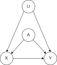
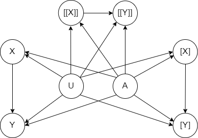
fig:triplet [SCM]  [triplet model]  [mutilated triplet model]

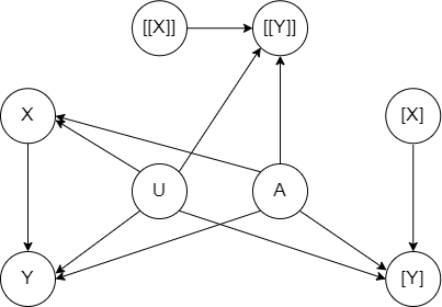
Figure 1: Reducing the counterfactual probability ${\it Pr}(y_{x},y_{x^{\prime}}^{\prime}|x,y)$ on the model in (a) to an observational probability ${\it Pr}([y],[[y^{\prime}]]\mid[x],[[x^{\prime}]],x,y)$ on the model in (c).

3 Causal Objective Functions and Unit Selection

A causal objective function can be any expression that involves observational, interventional or counterfactual probabilities where the goal of unit selection is to find objects (units) that optimize this function. However, inspired by (Li and Pearl, 2019), our treatment will be based on a specific class of causal objective functions which is a linear combination of counterfactual probabilities of the form ${\it Pr}({{\bf y}^{i}}_{{\bf x}^{i}},{{\bf w}^{i}}_{{\bf v}^{i}}|{\bf e}^{i},{\bf u})$ where $i=1,\ldots,n$. We call ${\bf U}$ the unit variables since our goal is to find instantiations ${\bf u}$ of these variables (i.e., units) that optimize the objective function. Variables ${\bf X}^{i}{\bf V}^{i}$ represent treatments, variables ${\bf Y}^{i}{\bf W}^{i}$ represent outcomes, $({\bf X}^{i}\cup{\bf V}^{i})\cap({\bf Y}^{i}\cup{\bf W}^{i})=\emptyset$, and variables ${\bf E}^{i}$ represent evidence. Unit variables are shared by all components of the objective function but each component can have its own treatment, outcome and evidence variables.

We will further assume that unit variables ${\bf U}$ are exogenous in the SCM (i.e., root variables) while treatment, outcome and evidence variables are endogenous. However, not all exogenous variables need to be unit variables. This is consistent with the assumption in (Li and Pearl, 2022a) that unit variables (also called characteristics) cannot be descendants of treatment or outcome variables. This leads us to objective functions of the following form:

$$L({\bf u})=\sum_{i=1}^{n}w_{i}\cdot{\it Pr}({\bf y}^{i}_{{\bf x}^{i}},{\bf w}^{i}_{{\bf v}^{i}}|{\bf e}^{i},{\bf u})\quad\text{where\ }w_{i}\geq 0\text{\ and\ }\sum_{i=1}^{n}w_{i}=1$$ (1)

We can now formally define the unit selection inference problem on structural causal models.

Definition 3.1 (Unit Selection).

Given an SCM $G$, a subset ${\bf U}$ of its variables, and an objective function $L({\bf u})$ such as eqn:objective-function, the unit selection inference problem is to compute $\operatornamewithlimits{argmax}_{\bf u}L({\bf u})$.

The benefit function discussed in (Li and Pearl, 2019) has the following form:

$$L(u)=\beta{\it Pr}(y_{x},y_{x^{\prime}}^{\prime}|u)+\gamma{\it Pr}(y_{x},y_{x^{\prime}}|u)+\theta{\it Pr}(y_{x}^{\prime},y_{x^{\prime}}^{\prime}|u)+\delta{\it Pr}(y_{x}^{\prime},y_{x^{\prime}}|u)$$ (2)

This class of objective functions falls as a special case of eqn:objective-function by setting $n=4$, ${\bf E}^{i}=\emptyset$, ${\bf X}^{i}={\bf V}^{i}=\{X\}$ and ${\bf Y}^{i}={\bf W}^{i}=\{Y\}$ for $i=1,\ldots,4$, where $X,Y$ are binary variables. That is, each component $i$ of the objective function uses the same single, treatment variable $X$ and the same single, outcome variable $Y$. A more general form was proposed in (Li and Pearl, 2022b) in which treatment $X$ has values $x_{1},\ldots,x_{m}$ and outcome $Y$ has values $y_{1},\ldots,y_{k}$ so the objective function can have up to $k^{m}$ components, each corresponding to a distinct response type such as ${\it Pr}({y_{2}}_{x_{1}},{y_{1}}_{x_{2}},{y_{1}}_{x_{3}},{y_{3}}_{x_{4}},{y_{2}}_{x_{5}}|u)$ when $k=3$ and $m=5$. This class of objective functions is more general than eqn:objective-function in that it allows one to express more response types but it assumes one treatment variable and one outcome variable. The class of objective functions we consider in eqn:objective-function allows compound treatments and outcomes. It also allows us to seek units from a particular group. For example, if $A$ and $B$ are two medications (binary treatments) and $T$ and $P$ refer to high temperature and high blood pressure (binary outcomes), and $E$ is the age group with values $e_{1},\ldots,e_{4}$, then the objective function can include terms such as ${\it Pr}({(t,p^{\prime})}_{a,b}\ ,\ {(t^{\prime},p^{\prime})}_{a^{\prime},b}\mid e_{3},u)$, which is the probability that a member of the third age group would have high temperature and normal blood pressure if administered both medications and would have normal temperature and blood pressure if administered only the second medication. Moreover, since the objective function components can have different treatment and outcome variables, one can select units based on their responses to distinct stimuli (e.g., effect of one type of encouragement on membership renewal and the simultaneous effect of another type of encouragement on increased purchases).

4 The Complexity of Unit Selection

We show next that unit selection is $\text{NP}^{\text}{PP}$-complete for the class of causal objective functions given in eqn:objective-function. We also show that this problem is $\text{NP}$-complete when unit variables correspond to all exogenous variables in the SCM. We start by providing an efficient reduction from unit selection into a variant of the well-known MAP inference problem, which we call Reverse-MAP. We then follow by studying the complexity of Reverse-MAP and unit selection.

Recall that our goal is to find units ${\bf u}$ that maximize the value $L({\bf u})$ of the objective function. The first step in solving this optimization problem is to be able to evaluate the objective $L({\bf u})$. We next show a construction which allows us to evaluate $L({\bf u})$ by evaluating a single observational probability involving unit variables ${\bf U}$ but on an extended and mutilated model. This construction will serve two purposes. First, it will permit us to characterize the complexity of unit selection when using objective functions in the form of eqn:objective-function. Second, we will later use the construction to develop a specific algorithm for solving the unit selection problem using these objective functions.

Consider each term ${\it Pr}({\bf y}^{i}_{{\bf x}^{i}},{\bf w}^{i}_{{\bf v}^{i}}|{\bf e}^{i},{\bf u})$ in eqn:objective-function. We reviewed in sec:background how this quantity can be reduced to a classical conditional probability on a triplet model $G^{i}$. The next step is to encode a linear combination of these conditional probabilities as a conditional probability on some model $G^{\prime}$. This is done using the following construction.

Definition 4.1 (Objective Model).

Consider an SCM $G$ with parameters $\theta$ and the objective function $L$ in eqn:objective-function. The objective model $G’$ for $\langle G,L\rangle$ has parameters $\theta^{\prime}$ and constructed as follows:

1. Construct a triplet model $G^{i}$ of $G$ for each term ${\it Pr}({\bf y}^{i}_{{\bf x}^{i}},{\bf w}^{i}_{{\bf v}^{i}}|{\bf e}^{i},{\bf u})$ in $L$ (see sec:background). Join $G^{1},\ldots,G^{n}$ so that their unit variables ${\bf U}$ are shared. This leads to model $G^{\prime}$.

2. Add a node $H$ to $G^{\prime}$ as a parent of all outcome nodes ${\bf Z}=\{[{\bf Y}^{i}],[[{\bf W}^{i}]]\}^{n}_{i=1}$. Node $H$ has states $h_{1},\ldots,h_{n}$ and prior $\theta^{\prime}(h_{i})=w_{i}$. Each node $Z\in{\bf Z}$ now has parents ${\bf P}_{Z}\cup\{H\}$, where ${\bf P}_{Z}$ are the parents of $Z$ in $G^{\prime}$ before node $H$ is added. Let $z^{i}$ be the state of $Z$ in the corresponding instantiation ${\bf y}^{i}{\bf w}^{i}$ of objective function $L$. The new CPT for $Z$ is:

   ${\bf P}_{Z}$	$H$	$Z$	$\theta^{\prime}(Z|{\bf P}_{Z},H)$
   ${\bf p}$	$h_{i}$	$z^{i}$	$\theta(z^{i}|{\bf p})$
   ${\bf p}$	$h_{i}$	$\bar{z}^{i}$	$\theta(\bar{z}^{i}|{\bf p})$
   ${\bf p}$	$\bar{h}_{i}$	$z^{i}$	$1.0$
   ${\bf p}$	$\bar{h}_{i}$	$\bar{z}^{i}$	$0.0$

   Here, $\bar{z}^{i},\bar{h}_{i}$ denote any states of variables $Z,H$ that are distinct from states $z^{i},h_{i}$.

We say the objective model $G^{\prime}$ has $n$ components, and call $H$ the mixture variable as it encodes a mixture of the objective function terms. The CPTs for variables $[{\bf Y}^{i}],[[{\bf W}^{i}]]$ in model $G^{\prime}$ reduce to their original CPTs in SCM $G$ when $H=h_{i}$, and imply $[{\bf Y}^{i}]={\bf y}^{i},[[{\bf W}^{i}]]={\bf w}^{i}$ when $H\neq h_{i}.$ The objective $L({\bf u})$ in SCM $G$ is a classical probability in the objective model $G^{\prime}$ (proof in app:reduction proof).

Theorem 4.2.

Consider an SCM $G$ with unit variables ${\bf U}$. Let $L$ be the objective function in eqn:objective-function, and let $G^{\prime}$ be an objective model for $\langle G,L\rangle$. Let ${\bf X}=\{[{\bf X}^{i}]\}_{i=1}^{n}$,${\bf Y}=\{[{\bf Y}^{i}]\}_{i=1}^{n}$, ${\bf W}=\{[[{\bf W}^{i}]]\}_{i=1}^{n}$, ${\bf V}=\{[[{\bf V}^{i}]]\}_{i=1}^{n}$ and ${\bf E}=\{{\bf E}^{i}\}_{i=1}^{n}$. We have $L({\bf u})={\it Pr}^{\prime}({\bf y},{\bf w}|{\bf x},{\bf v},{\bf e},{\bf u}),$ where ${\bf y},{\bf w},{\bf x},{\bf v},{\bf e}$ are the instantiations of variables ${\bf Y},{\bf W},{\bf X},{\bf V},{\bf E}$ in objective function $L$.

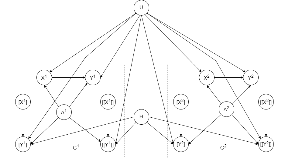
Figure 2: An objective model with two components for the SCM in fig:base-triplet.

Consider the SCM in fig:base-triplet and the causal objective function $L(u)=w_{1}\cdot{\it Pr}(y_{x},y^{\prime}_{x^{\prime}}|u)+w_{2}\cdot{\it Pr}(y_{x},y_{x^{\prime}}|u)$. Figure 2 shows a corresponding objective model $G^{\prime}$ constructed according to Definition 4.1. We now have $L(u)={\it Pr}^{\prime}([y^{1}],[[{y^{\prime}}^{1}]],[y^{2}],[[y^{2}]]\mid[x^{1}],[[{x^{\prime}}^{1}]],[x^{2}],[[{x^{\prime}}^{2}]],u).$

Theorem 4.2 suggests that we can optimize the objective function $L({\bf u})$ on an SCM $G$ by computing the instantiation $\operatornamewithlimits{argmax}_{\bf u}{\it Pr}({\bf y},{\bf w}|{\bf x},{\bf v},{\bf e},{\bf u})$ on an objective model $G^{\prime}$. The is similar to the classical MAP problem on model $G^{\prime}$, except that the optimized variables ${\bf U}$ appear after the conditioning operator instead of before it. This leads to our definition of the Reverse-MAP problem.

Definition 4.3 (Reverse-MAP).

Consider an SCM $G$ with distribution ${\it Pr}$ and suppose ${\bf U},{\bf E}_{1},{\bf E}_{2}$ are disjoint sets of variables in $G$. The Reverse-MAP instantiation for variables ${\bf U}$ and instantiations ${\bf e}_{1},{\bf e}_{2}$ is defined as follows: $\rmap({\bf U},{\bf e}_{1},{\bf e}_{2})\triangleq\operatornamewithlimits{argmax}_{{\bf u}}{\it Pr}({\bf e}_{1}\mid{\bf u},{\bf e}_{2}).$

To see the connection between Reverse-MAP and MAP, note that $\operatornamewithlimits{argmax}_{{\bf u}}{\it Pr}({\bf e}_{1}|{\bf u},{\bf e}_{2})=\operatornamewithlimits{argmax}_{{\bf u}}{\it Pr}({\bf u},{\bf e}_{1},{\bf e}_{2})/{\it Pr}({\bf u},{\bf e}_{2})$ where $\operatornamewithlimits{argmax}_{{\bf u}}{\it Pr}({\bf u},{\bf e}_{1},{\bf e}_{2})=\operatornamewithlimits{argmax}_{{\bf u}}{\it Pr}({\bf u}|{\bf e}_{1},{\bf e}_{2})$ is the known MAP problem (Pearl, 1989). In general, the MAP instantiation $\operatornamewithlimits{argmax}_{{\bf u}}{\it Pr}({\bf u},{\bf e}_{1},{\bf e}_{2})$ is not the Reverse-MAP instantiation since ${\it Pr}({\bf u},{\bf e}_{2})$ also depends on ${\bf U}$; see app:example-map-rmap for a concrete example that illustrates this point. We now have the following result, proven in app:poly reductions proof.

Corollary 4.4.

There are polynomial-time reductions between the Reverse-MAP problem and the unit selection problem with objective functions in the form of eqn:objective-function.

We next characterize the complexity of Reverse-MAP under different conditions. Consider a decision version of the problem, D-Reverse-MAP, defined as follows.

Definition 4.5 (D-Reverse-MAP).

Given an SCM with rational parameters that induces distribution ${\it Pr}$, some target variables ${\bf U}$, some evidence ${\bf e}_{1},{\bf e}_{2}$ and a rational threshold $p$, the D-Reverse-MAP problems asks whether there is an instantiation ${\bf u}$ of ${\bf U}$ such that ${\it Pr}({\bf e}_{1}|{\bf u},{\bf e}_{2})>p$.

The next theorem shows that D-Reverse-MAP is $\text{NP}^{\text}{PP}$-complete, like classical MAP (Park and Darwiche, 2004b). Its proof can be found in app:d-reverse-map proof NP-PP.

Theorem 4.6.

D-Reverse-MAP is $\text{NP}^{\text}{PP}$-complete.

We can now characterize the complexity of unit selection using thm:D-Reverse-MAP complexity and cor:unit-selection-rmap.

Corollary 4.7.

Unit selection is $\text{NP}^{\text}{PP}$-complete assuming the objective function in eqn:objective-function.

In an SCM, exogenous (root) variables represent all uncertainties in the model and the endogenous (internal) variables are uniquely determined by exogenous variables. This property of SCMs significantly reduces the complexity of unit selection when the unit variables correspond to all SCM exogenous variables. This is implied by the following result which is proven in app:d-reverse-map proof NP.

Theorem 4.8.

D-Reverse-MAP is $\text{NP}$-complete if its target variables are all the SCM root variables.

Corollary 4.9.

Unit selection is $\text{NP}$-complete when the unit variables are all the SCM exogenous (root) variables, assuming the objective functions in eqn:objective-function.

5 Unit Selection using Variable Elimination

sec:unit-selection-reduction provided a reduction from unit selection on an SCM to Reverse-MAP on an objective model. In sec:ve, we provide a variable elimination (VE) algorithm for Reverse-MAP which can be applied to the objective model to solve unit selection. In sec:treewidth bounds, we analyze the complexity of this method and compare it to the complexity of Reverse-MAP on the underlying SCM.

5.1 Reverse-MAP using Variable Elimination

Our VE algorithm for Reverse-MAP will employ the same machinery and techniques used in the VE algorithm for classical MAP (Dechter, 1999). Hence, we will first review the VE algorithm for MAP using the treatment in (Darwiche, 2009, Ch 10) and then discuss the algorithm for Reverse-MAP.

The VE algorithm is based on the notion of a factor $f({\bf X})$ which maps each instantiation ${\bf x}$ of variables ${\bf X}$ into a non-negative number $f({\bf x})$. VE employs a number of factor operations including multiplying two factors ($f\cdot g$), summing out a variable from a factor ($\sum_{X}f$), maximizing out a variable from a factor ($\max_{X}f$), and dividing two factors ($f/g$). Let $G$ be an SCM and assume its variables ${\bf Z}$ are partitioned into three disjoint sets ${\bf U},{\bf V},{\bf E}$, where ${\bf U}$ are the target variables and ${\bf E}$ are the evidence variables. Let ${\bf S}={\bf Z}\setminus{\bf U}$ in the following discussion. We will treat the CPT of each variable $Z$ in SCM $G$ as a factor over $Z$ and its parents ${\bf P}$, denoted $f_{Z}(Z{\bf P})$. The SCM distribution is then ${\it Pr}({\bf Z})=\prod_{Z\in{\bf Z}}f_{Z}$. We capture evidence ${\bf e}$ by creating an evidence factor $\lambda_{e}(E)$ for each $e\in{\bf e}$ with $\lambda_{e}(e^{\prime})=1$ if $e^{\prime}=e$ and $\lambda_{e}(e^{\prime})=0$ otherwise. The MAP probability is then given by

$$\map_{p}({\bf U},{\bf e})=\max_{\bf u}{\it Pr}({\bf u},{\bf e})=\max_{\bf u}\sum_{\bf v}{\it Pr}({\bf u},{\bf v},{\bf e})=\max_{{\bf U}}\sum_{{\bf S}}\prod_{Z\in{\bf Z}}f_{Z}\prod_{e\in{\bf e}}\lambda_{e}(E)$$ (3)

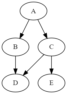
Figure 3: SCM

This is in contrast to the MAP instantiation which is $\operatornamewithlimits{argmax}_{\bf u}{\it Pr}({\bf u},{\bf e})$. With some minor bookkeeping, the VE algorithm for computing the MAP probability can also return a MAP instantiation; see, e.g., (Darwiche, 2009, Ch 10). Hence, we will focus next on computing the MAP probability.

Consider the SCM in fig:ve-scm and suppose ${\bf U}=\{A,B\}$ and the evidence ${\bf e}$ is $\{E=e\}$. In this case, $\map_{p}(AB,e)$ will be equal to

$$\max_{AB}\sum_{CDE}f_{A}(A)f_{B}(AB)f_{C}(AC)f_{D}(BCD)f_{E}(CE)\lambda_{e}(E)$$ (4)

Algorithm 1 MAP_VE$(G,{\bf U},{\bf e})$

Input: SCM $G$, target variables ${\bf U}$, evidence ${\bf e}$
      Output: scalar factor containing $\map_{p}({\bf U},{\bf e})$

1:procedure main

2:    $\pi_{\bf S}\leftarrow$ an elimination order for non-target variables

3:    $\pi_{\bf U}\leftarrow$ an elimination order for target variables ${\bf U}$

4:    $\mathcal{F}\leftarrow\{f:f\mbox{ is a CPT of SCM }G\}\cup\{\lambda_{e}:\lambda_{e}\mbox{ is an evidence factor for }e\in{\bf e}\}$

5:    ${\cal G}\leftarrow$ eliminate($\sum,\mathcal{F},\pi_{\bf S}$)

6:    $p\leftarrow$ eliminate($\max,{\cal G},\pi_{\bf U}$)

7:    return $p$

8:end procedure

Input: an operation $\bigcirc\in\{\sum,\max\}$, a set of factors $\mathcal{F}$, a total variable order $\pi$
      Output: a set of factors

Algorithm 2 Eliminating Variables using Sum or Max

1:procedure eliminate($\bigcirc,\mathcal{F},\pi$)

2:    for $i=1$ to length of order $\pi$ do

3:         $V\leftarrow i^{th}$ variable in order $\pi$

4:         ${\cal G}\leftarrow$ factors in $\mathcal{F}$ that mention variable $V$

5:         $f_{i}\leftarrow\prod_{f\in{\cal G}}f$

6:         $f_{i}\leftarrow\bigcirc_{V}f_{i}$

7:         replace factors $\cal G$ in $\mathcal{F}$ with factor $f_{i}$

8:    end for

9:    return $\mathcal{F}$

10:end procedure

A naive evaluation of this expression multiplies all factors to yield a factor $f(ABCDE)$ over all variables, then computes $\max_{AB}\sum_{CDE}f(ABCDE)$, leading to $O(n\exp(n))$ complexity where $n$ is the number of model variables. The VE algorithm tries to compute this expression more efficiently with pseudocode provided in alg:ve-map (MAP_VE). The product of factors $\mathcal{F}$ on Line 4 represents the joint distribution ${\it Pr}({\bf Z},{\bf e})$ so we first sum out variables ${\bf S}$ from $\mathcal{F}$ on Line 5 to compute a set of factors ${\cal G}$ whose product represents the marginal ${\it Pr}({\bf U},{\bf e})$. We then maximize out variables ${\bf U}$ from $\cal G$ on Line 6 leading to a scalar factor $p$ that contains the MAP probability (see Footnote 7). alg:ve-map eliminates variables one by one using alg:eliminate and a total variable order $\pi=\langle\pi_{\bf S},\pi_{\bf U}\rangle$, known as an elimination order. MAP_VE requires variables ${\bf U}$ to appear last in order $\pi$ since summation does not commute with maximization. An order that satisfies this constraint is known as a ${\bf U}$-constrained elimination order. The complexity of MAP_VE depends on the used elimination order $\pi$. In each elimination step of alg:eliminate, we multiply all factors that mention variable $\pi(i)$ to obtain factor $f_{i}$ on Line 6. The variables in $f_{i}$ are called a cluster ${\bf C}_{i}$ so eliminating variables $\pi(1),\ldots,\pi(n)$ induces clusters ${\bf C}_{1},\ldots,{\bf C}_{n}.$ The width $w$ of elimination order $\pi$ is the size of largest cluster minus one and the complexity of MAP_VE is $O(n\exp(w))$.

The table below depicts the trace of MAP_VE when computing the MAP probability in eqn:map-expression using the elimination order $\pi=E,D,C,B,A$. The trace shows that MAP_VE evaluates the following factorized expression and that the width of order $\pi$ is $2$ (largest cluster has size $3$):

$$\map_{p}(AB,e)=\max_{A}f_{A}(A)\left[{\max_{B}f_{B}(AB)\left[{\sum_{C}f_{C}(AC)\left[{\sum_{D}f_{D}(BCD)\left[{\sum_{E}f_{E}(CE)\lambda_{E}}\right]}\right]}\right]}\right]$$

$i$	eliminated var	factors $\cal G$ (Line 4, alg:eliminate)	new factor $f_{i}$ (Line 6, alg:eliminate)	${\bf C}_{i}$
$1$	$E$	$f_{E}(CE)\ \lambda_{E}$	$f_{1}=\sum_{E}f_{E}(CE)\ \lambda_{E}$	CE
$2$	$D$	$f_{D}(BCD)$	$f_{2}=\sum_{D}f_{D}(BCD)$	BCD
$3$	$C$	$f_{C}(AC)\ f_{1}(C)\ f_{2}(BC)$	$f_{3}=\sum_{C}f_{C}(AC)\ f_{1}(C)\ f_{2}(BC)$	ABC
$4$	$B$	$f_{B}(AB)\ f_{3}(AB)$	$f_{4}=\max_{B}f_{B}(AB)\ f_{3}(AB)$	AB
$5$	$A$	$f_{A}(A)\ f_{4}(A)$	$p=\max_{A}f_{A}(A)\ f_{4}(A)$	A

Choosing a good elimination order is critical for the complexity of VE. The treewidth of an SCM $G$ is defined as the minimum width attained by any elimination order. Since MAP requires ${\bf U}$-constrained orders, the ${\bf U}$-constrained treewidth of $G$ is defined as the minimum width attained by any ${\bf U}$-constrained elimination order (Park and Darwiche, 2004b).

We are now ready to introduce our VE algorithm for Reverse-MAP. Again, we assume that the model variables ${\bf Z}$ are partitioned into disjoint sets ${\bf U},{\bf V},{\bf E}$, where ${\bf U}$ are the target variables and ${\bf S}={\bf Z}\setminus{\bf U}$. But we further partition the evidence variables ${\bf E}$ into ${\bf E}_{1}$ and ${\bf E}_{2}$. Again, we focus on computing the Reverse-MAP probability $\rmap_{p}({\bf U},{\bf e}_{1},{\bf e}_{2})$ instead of the instantiation:

$$\max_{\bf u}{\it Pr}({\bf e}_{1}|{\bf u},{\bf e}_{2})=\frac{{\it Pr}({\bf u},{\bf e}_{1},{\bf e}_{2})}{{\it Pr}({\bf u},{\bf e}_{2})}=\frac{\sum_{\bf v}{\it Pr}({\bf u},{\bf v},{\bf e}_{1},{\bf e}_{2})}{\sum_{\bf v}{\it Pr}({\bf u},{\bf v},{\bf e}_{2})}=\max_{{\bf U}}\frac{\displaystyle\sum_{{\bf S}}\prod_{Z\in{\bf Z}}f_{Z}\prod_{e\in{\bf e}_{1}\cup{\bf e}_{2}}\lambda_{e}}{\displaystyle\sum_{{\bf S}}\prod_{Z\in{\bf Z}}f_{Z}\prod_{e\in{\bf e}_{2}}\lambda_{e}}$$

Our algorithm, called RMAP_VE, runs two passes of elimination as shown in alg:ve-rmap. In the first pass (Line 4), we sum out variables ${\bf S}$ under evidence ${\bf e}_{1},{\bf e}_{2}$ and in the second pass (Line 5), we sum out variables ${\bf S}$ under evidence ${\bf e}_{2}$. This leads to two sets of factors ${\cal G}_{1}$ and ${\cal G}_{2}$ which correspond to marginal distributions ${\it Pr}({\bf U},{\bf e}_{1},{\bf e}_{2})$ and ${\it Pr}({\bf U},{\bf e}_{2})$. Now we need to divide ${\it Pr}({\bf U},{\bf e}_{1},{\bf e}_{2})$ and ${\it Pr}({\bf U},{\bf e}_{2})$ to compute ${\it Pr}({\bf e}_{1}|{\bf U},{\bf e}_{2})$. We next show that this can be done efficiently by “dividing” ${\cal G}_{1}$ and ${\cal G}_{2}$ as shown on Line 8. The key idea is that if we run the two passes of elimination according to the same elimination order, then there will be a one-to-one correspondence between the factors in ${\cal G}_{1}$ and ${\cal G}_{2}$. Let $(g_{1}^{i},g_{2}^{i})$ be the corresponding pairs of factors for $i=1,\ldots,k$ where $k=|{\cal G}_{1}|=|{\cal G}_{2}|$. What we need is $\left(\prod_{i=1}^{n}g_{1}^{i}\right)/\left(\prod_{i=1}^{n}g_{2}^{i}\right)$ since this represents ${\it Pr}({\bf e}_{1}|{\bf U},{\bf e}_{2})$. But due to the mentioned correspondence, this equals $\prod_{i=1}^{n}g_{1}^{i}/g_{2}^{i}$. Thus, we can divide each pair of corresponding factors to obtain the set of factors ${\cal G}$ as done on Line  8. We finally maximize out target variables ${\bf U}$ from ${\cal G}$ to obtain the Reverse-MAP probability (Line 9).

Algorithm 3 RMAP_VE($G,{\bf U},{\bf e}_{1},{\bf e}_{2})$

Input: SCM $G$, target variables ${\bf U}$, evidence ${\bf e}_{1}$ and ${\bf e}_{2}$
      Output: scalar factor containing $\rmap_{p}({\bf U},{\bf e}_{1},{\bf e}_{2})$

1:procedure main

2:    $\pi_{\bf S}\leftarrow$ an elimination order for non-target variables

3:    $\pi_{\bf U}\leftarrow$ an elimination order for target variables ${\bf U}$

4:    $\mathcal{F}_{1}\leftarrow\{f:f\mbox{ is a CPT of SCM }G\}\cup\{\lambda_{e}:\lambda_{e}\mbox{ is an evidence factor for }e\in{\bf e}_{1},{\bf e}_{2}\}$

5:    $\mathcal{F}_{2}\leftarrow\{f:f\mbox{ is a CPT of SCM }G\}\cup\{\lambda_{e}:\lambda_{e}\mbox{ is an evidence factor for }e\in{\bf e}_{2}\}$

6:    ${\cal G}_{1}\leftarrow$ eliminate($\sum,\mathcal{F}_{1},\pi_{\bf S}$)

7:    ${\cal G}_{2}\leftarrow$ eliminate($\sum,\mathcal{F}_{2},\pi_{\bf S}$)

8:    ${\cal G}\leftarrow\{g_{1}/g_{2}:$ $g_{1},g_{2}$ are corresponding factors in ${\cal G}_{1},{\cal G}_{2}\}$

9:    $p\leftarrow$ eliminate($\max,{\cal G},\pi_{\bf U}$)

10:    return $p$

11:end procedure

RMAP_VE has the same complexity as MAP_VE if both use the same elimination order. Suppose there are $k$ factors in ${\cal G}_{1}/{\cal G}_{2}/{\cal G}$ and the largest factor has size $c$. The cost of division on Line 8 is $O(k\exp(c))$ while the cost of maximization on Line 9 is at least $O(k\exp(c))$ so the cost of division is dominated by the cost of maximization. Hence, the complexity of RMAP_VE is still $O(n\exp(w))$ where $n$ is the number of variables and $w$ is the width of used ${\bf U}$-constrained order $\pi$.

5.2 Bounding the Complexity of Unit Selection using Variable Elimination

We can solve unit selection by applying RMAP_VE to an objective model of the SCM as shown by thm:unit-selection-reduction. However, RMAP_VE (and MAP_VE) is expected to be more expensive on the objective model compared to the given SCM since the former is larger and denser than the latter. But how much more expensive? In particular, is RMAP_VE always tractable on the objective model when it is tractable on the underlying SCM? We consider this question next using the lens of treewidth which is commonly used to analyze elimination algorithms. Recall also that MAP_VE and RMAP_VE have the same complexity when applied to the same SCM using the same target variables.

Our starting point is to study the treewidth of an objective model in relation to the treewidth of its underlying SCM. We will base our study on the techniques and results reported in (Han et al., 2022) which studied the complexity of counterfactual reasoning. In particular, given an elimination order $\pi$ of SCM $G$, we next show how to construct an elimination order $\pi^{\prime}$ for the objective model $G^{\prime}$ while providing a bound on the width of order $\pi^{\prime}$ in terms of the width of order $\pi$. Recall that we use $[X]$ and $[[X]]$ to denote the copies of variable $X$ in a triplet model where $X=[X]=[[X]]$ if $X$ is exogenous. Moreover, if $U$ is a unit variable, then $U=U^{1}=\cdots=U^{n}$ in an objective model.

Definition 5.1.

Let $G$ be an SCM and $G^{\prime}$ be a corresponding objective model with $n$ components. If $\pi$ is an elimination order for $G$, the corresponding elimination order $\pi^{\prime}$ for $G^{\prime}$ is obtained by replacing each non-unit variable $X$ in $\pi$ by $X^{1},\ldots,X^{n},[X^{1}],\ldots,[X^{n}],[[X^{1}]],\ldots,[[X^{n}]]$ then appending the mixture variable $H$ to the end of the order.

Consider the elimination order $\pi=A,X,Y,U$ for the SCM in fig:base-triplet. The corresponding elimination order $\pi^{\prime}$ for the objective model in fig:objective model is as follows:

$$\pi^{\prime}=A^{1},A^{2},X^{1},X^{2},[X^{1}],[X^{2}],[[X^{1}]],[[X^{2}]],Y_{1},Y_{2},[Y_{1}],[Y_{2}],[[Y_{1}]],[[Y_{2}]],U,H$$

The following bound (thm:objective-width) follows from lem:add-node and Theorem 5.3 which concerns $n$-world models. Given an SCM $G$ and a subset ${\bf U}$ of its roots, an $n$-world model is obtained by creating $n$ copies of $G$ that share nodes ${\bf U}$ (Han et al., 2022). This notion corresponds to parallel worlds models (Avin et al., 2005) when ${\bf U}$ contains all roots of SCM $G$. An objective model with $n$ components can be viewed as a $3n$-world model but with an additional mixture node $H$ and some edges that originate from $H$. lem:add-node and thm:objective-width are proven in app:lemma-add-node and app:objective width.

Lemma 5.2.

Consider an SCM $G$ and suppose SCM $G^{\prime}$ is obtained from $G$ by adding a root node $H$ as a parent of some nodes in $G$. If $\pi$ is an elimination order for $G$ and has width $w$, then $\pi^{\prime}=\langle\pi,H\rangle$ is an elimination order for $G^{\prime}$ and has width $w^{\prime}\leq w+1$.

Theorem 5.3 (Han et al. (2022)).

Consider an SCM $G$, a subset ${\bf U}$ of its roots and a corresponding $n$-world model $G^{\prime}$. If $G$ has an elimination order $\pi$ with width $w$, then there exists a corresponding elimination order $\pi^{\prime}$ of $G^{\prime}$ that has width $w^{\prime}\leq n(w+1)-1$.

Theorem 5.4.

Consider an SCM $G$ and a corresponding objective model $G^{\prime}$ with $n$ components. Let $\pi$ be an elimination order for $G$ and let $\pi^{\prime}$ be the corresponding elimination order for $G^{\prime}$. If $\pi$ has width $w$ and $\pi^{\prime}$ has width $w^{\prime}$, then $w^{\prime}\leq 3n(w+1)$.

Corollary 5.5.

If $w$ is the treewidth of an SCM $G$ and $w^{\prime}$ is the treewidth of a corresponding objective model $G^{\prime}$ with $n$ components, then $w^{\prime}\leq 3n(w+1)$.

As mentioned earlier, RMAP_VE and MAP_VE require a ${\bf U}$-constrained elimination orders in which unit variables ${\bf U}$ appear last in the order. Hence, a ${\bf U}$-constrained elimination order for an objective model must place the mixture variable $H$ before ${\bf U}$. This leads to the next definition.

Definition 5.6.

Let $G$ be an SCM with unit variables ${\bf U}$ and let $G^{\prime}$ be a corresponding objective model with $n$ components. If $\pi$ is a ${\bf U}$-constrained elimination order for $G$, the corresponding ${\bf U}$-constrained elimination order $\pi^{\prime}$ for $G^{\prime}$ is obtained by replacing each non-unit variable $X$ in $\pi$ by $X^{1},\ldots,X^{n},[X^{1}],\ldots,[X^{n}],[[X^{1}]],\ldots,[[X^{n}]]$ then inserting mixture variable $H$ just before ${\bf U}$.

Consider the ${\bf U}$-constrained order $\pi=A,X,Y,U$ for the SCM in fig:base-triplet. The corresponding ${\bf U}$-constrained elimination order for the objective model in fig:objective model is

$$\pi^{\prime}=A^{1},A^{2},X^{1},X^{2},[X^{1}],[X^{2}],[[X^{1}]],[[X^{2}]],Y_{1},Y_{2},[Y_{1}],[Y_{2}],[[Y_{1}]],[[Y_{2}]],H,U$$

We now have the following bound on the ${\bf U}$-constrained treewidth of objective models, which is somewhat unexpected when compared to the bound on treewidth. In particular, while the bound on treewidth grows linearly in the number of components in the objective model, the bound on ${\bf U}$-constrained treewidth is independent of such a number. Moreover, the bound on ${\bf U}$-constrained treewidth can depend on the number of unit variables which is not the case for treewidth.

Theorem 5.7.

Let $G$ be an SCM with unit variables ${\bf U}$ and let $G^{\prime}$ be a corresponding objective model. If $\pi$ is a ${\bf U}$-constrained elimination order for $G$ with width $w$ and $\pi^{\prime}$ is the corresponding ${\bf U}$-constrained elimination order for $G^{\prime}$ with width $w^{\prime}$, then $w^{\prime}\leq\max(3w+3,|{\bf U}|)$. If the objective function in eqn:objective-function has one outcome variable (${\bf Y}^{i}={\bf W}^{i}=\{Y\}$ for all $i$), then $w^{\prime}\leq 3w+3$.

Corollary 5.8.

Let $G$ be an SCM with unit variables ${\bf U}$ and let $G^{\prime}$ be a corresponding objective model. If $w$ and $w^{\prime}$ are the ${\bf U}$-constrained treewidths of $G$ and $G^{\prime}$, then $w^{\prime}\leq\max(3w+3,|{\bf U}|)$. Moreover, if the objective function in eqn:objective-function has a single outcome variable, then $w^{\prime}\leq 3w+3$.

The above bounds can be significantly tighter depending on the objective function properties. cor:objective-constrained-treewidth identifies one such property which is satisfied by the benefit function in (Li and Pearl, 2019); see Equation eqn:benefit-ang. Moreover, the factor $3$ in these bounds is an implication of using a triplet model which may not be necessary. Consider components ${\it Pr}({\bf y}^{i}_{{\bf x}^{i}},{\bf w}^{i}_{{\bf v}^{i}}|{\bf e}^{i},{\bf u})$ in the objective function of eqn:objective-function. If ${\bf E}^{i}\!\!=\!\!\emptyset$ for all $i$, then a twin model is sufficient when building an objective model (similarly if ${\bf Y}^{i}\!\!=\!\!{\bf X}^{i}\!\!=\!\!\emptyset$ or ${\bf W}^{i}\!\!=\!\!{\bf V}^{i}\!\!=\!\!\emptyset$). The objective function in Equation eqn:benefit-ang, from (Li and Pearl, 2019), has ${\bf E}^{i}\!\!=\!\!\emptyset$ for all $i$ so it leads to the tighter bound $w^{\prime}\leq 2w+2$. More generally, if the objective function properties lead to removing the dependence on $|{\bf U}|$ in the bound of cor:objective-constrained-treewidth, then RMAP_VE on an objective model is tractable if RMAP_VE (MAP_VE) is tractable on the underlying SCM. Otherwise, the bound in cor:objective-constrained-treewidth does not guarantee this. Recall that MAP, Reverse-MAP and unit selection using eqn:objective-function are all $\text{NP}^{\text}{PP}$-complete as shown earlier.

We provide in Appendix LABEL:app:experiment a preliminary experiment and an extensive discussion in relation to the complexities of three algorithms: (1) MAP_VE (Algorithm 1) which solves MAP by operating on an SCM; (2) RMAP_VE (Algorithm 3) which solves unit selection by operating on an objective model; and (3) a baseline, bruteforce method which solves unit selection by operating on a twin or triplet model (depending on the objective function). The main finding of the experiment is that, as the size of the problem grows, the gap between the complexities of MAP_VE and RMAP_VE narrows while the gap between the complexities of RMAP_VE and the bruteforce method grows (the bruteforce method is significantly worse and becomes impractical pretty quickly).

Appendix LABEL:app:experiment also identifies a class of SCM structures (and unit variables) for which the number of unit variables is unbounded but the complexity of RMAP_VE on an objective model is bounded.

6 Conclusion

We studied the unit selection problem in a computational setting which complements existing studies. We assumed a fully specified structural causal model so we can compute point values of causal objective functions, allowing us to entertain a broader class of functions than is normally considered. We showed that the unit selection problem with this class of objective functions is $\text{NP}^{\text}{PP}$-complete, similar to the classical MAP problem, and identified an intuitive condition under which it is $\text{NP}$-complete. We further provided an exact algorithm for the unit selection problem based on variable elimination and characterized its complexity in terms of treewidth, while relating this complexity to that of MAP inference. In the process, we defined a new inference problem, Reverse-MAP, which is also $\text{NP}^{\text}{PP}$-complete but captures the essence of unit selection more than MAP does.

We thank Yizuo Chen, Yunqiu Han, Ang Li and Scott Mueller for providing useful feedback on an earlier version of this paper. This work has been partially supported by ONR grant N000142212501.

Appendix A Proof of thm:unit-selection-reduction

The proof of this theorem requires a lemma which requires the following definition. We will say that a set of variables ${\bf Z}$ decomposes a DAG if removing the outgoing edges from ${\bf Z}$ splits the DAG into at least two disconnected components.

Lemma A.1.

Consider an SCM $G$ with distribution ${\it Pr}$ and three disjoint set of variables ${\bf X},{\bf Y},{\bf Z}$. Suppose ${\bf Z}$ decomposes $G$ into disconnected components $G_{1}$ and $G_{2}$. If ${\bf X}_{1},{\bf Y}_{1}$ are subsets of ${\bf X},{\bf Y}$ pertaining to $G_{1}$, and ${\bf X}_{2},{\bf Y}_{2}$ are subsets of ${\bf X},{\bf Y}$ pertaining to $G_{2}$, then ${\it Pr}({\bf y}|{\bf x},{\bf z})={\it Pr}({\bf y}_{1}|{\bf x}_{1},{\bf z}){\it Pr}({\bf y}_{2}|{\bf x}_{2},{\bf z})$.

Proof A.2.

Since ${\bf Z}$ decomposes $G$, we have $\dsep_{G}({\bf X}_{1},{\bf Z},{\bf X}_{2})$ and $\dsep_{G}({\bf X}_{1}{\bf Y}_{1},{\bf Z},{\bf X}_{2}{\bf Y}_{2})$. We have:

$${\it Pr}({\bf y}|{\bf x},{\bf z}) =\frac{{\it Pr}({\bf y},{\bf x}|{\bf z})}{{\it Pr}({\bf x}|{\bf z})}=\frac{{\it Pr}({\bf y}_{1},{\bf y}_{2},{\bf x}_{1},{\bf x}_{2}|{\bf z})}{{\it Pr}({\bf x}_{1},{\bf x}_{2}|{\bf z})}=\frac{{\it Pr}({\bf y}_{1},{\bf x}_{1}|{\bf z}){\it Pr}({\bf y}_{1},{\bf x}_{1}|{\bf z})}{{\it Pr}({\bf x}_{1}|{\bf z}){\it Pr}({\bf x}_{2}|{\bf z})}$$ (5)

$$=\left[\frac{{\it Pr}({\bf y}_{1},{\bf x}_{1}|{\bf z})}{{\it Pr}({\bf x}_{1}|{\bf z})}\right]\left[\frac{{\it Pr}({\bf y}_{2},{\bf x}_{2}|{\bf z})}{{\it Pr}({\bf x}_{2}|{\bf z})}\right]={\it Pr}({\bf y}_{1}|{\bf x}_{1},{\bf z}){\it Pr}({\bf y}_{2}|{\bf x}_{2},{\bf z})$$

eqn:cutset follows from $\dsep_{G}({\bf X}_{1},{\bf Z},{\bf X}_{2})$ and $\dsep_{G}({\bf X}_{1}{\bf Y}_{1},{\bf Z},{\bf X}_{2}{\bf Y}_{2})$. This concludes our proof. Although we only consider the case of two subnetworks here, it is easy to see that this lemma generalizes to an arbitrary number of subnetworks decomposed by ${\bf Z}$.

We are now ready to prove thm:unit-selection-reduction. By construction of $G^{\prime}$, ${\bf U}\cup\{H\}$ decomposes $G^{\prime}$ into its $n$ components $G^{1},G^{2},\ldots G^{n}$. We have:

References

- Avin et al. (2005) Chen Avin, Ilya Shpitser, and Judea Pearl. Identifiability of path-specific effects. In IJCAI, pages 357–363. Professional Book Center, 2005.
- Balke and Pearl (1994) Alexander Balke and Judea Pearl. Probabilistic evaluation of counterfactual queries. In AAAI, pages 230–237. AAAI Press / The MIT Press, 1994.
- Balke and Pearl (1995) Alexander Balke and Judea Pearl. Counterfactuals and policy analysis in structural models. In UAI, pages 11–18. Morgan Kaufmann, 1995.
- Bareinboim et al. (2021) E. Bareinboim, Juan David Correa, D. Ibeling, and Thomas F. Icard. On Pearl’s hierarchy and the foundations of causal inference. 2021. Technical Report, R-60, Colombia University.
- Darwiche (2009) Adnan Darwiche. Modeling and Reasoning with Bayesian Networks. Cambridge University Press, 2009.
- Dawid et al. (2017) Philip Dawid, Monica Musio, and Rossella Murtas. The probability of causation. Law, Probability and Risk, 16(4):163–179, 2017.
- Dechter (1999) Rina Dechter. Bucket elimination: A unifying framework for reasoning. Artif. Intell., 113(1-2):41–85, 1999.
- Galles and Pearl (1998) David Galles and Judea Pearl. An axiomatic characterization of causal counterfactuals. Foundations of Science, 3(1):151–182, 1998.
- Halpern (2000) Joseph Y Halpern. Axiomatizing causal reasoning. Journal of Artificial Intelligence Research, 12:317–337, 2000.
- Han et al. (2022) Yunqiu Han, Yizuo Chen, and Adnan Darwiche. On the complexity of counterfactual reasoning. In A causal view on dynamical systems, NeurIPS 2022 workshop, 2022. URL https://arxiv.org/abs/2211.13447.
- Kjærulff (1990) Uffe Kjærulff. Triangulation of graphs - algorithms giving small total state space. Technical Report R 90-09, Department of Mathematics and Computer Science, Strandvejen, DK 9000 Aalborg, Denmark, 1990.
- Koller and Friedman (2009) Daphne Koller and Nir Friedman. Probabilistic Graphical Models - Principles and Techniques. MIT Press, 2009.
- Li et al. (2022a) A. Li, S. Jiang, Y. Sun, and J. Pearl. Learning probabilities of causation from finite population data. Technical Report R-519, http://ftp.cs.ucla.edu/pub/stat_ser/r519.pdf, Department of Computer Science, University of California, Los Angeles, CA, 2022a.
- Li and Pearl (2019) Ang Li and Judea Pearl. Unit selection based on counterfactual logic. In IJCAI, pages 1793–1799. ijcai.org, 2019.
- Li and Pearl (2022a) Ang Li and Judea Pearl. Unit selection with causal diagram. In AAAI, pages 5765–5772. AAAI Press, 2022a.
- Li and Pearl (2022b) Ang Li and Judea Pearl. Unit selection with nonbinary treatment and effect. CoRR, abs/2208.09569, 2022b.
- Li and Pearl (2022c) Ang Li and Judea Pearl. Unit selection: Case study and comparison with A/B test heuristic. CoRR, abs/2210.05030, 2022c.
- Li et al. (2022b) Ang Li, Song Jiang, Yizhou Sun, and Judea Pearl. Unit selection: Learning benefit function from finite population data. CoRR, abs/2210.08203, 2022b.
- Littman et al. (1998) Michael L Littman, Judy Goldsmith, and Martin Mundhenk. The computational complexity of probabilistic planning. Journal of Artificial Intelligence Research, 9:1–36, 1998.
- Mueller et al. (2021) S. Mueller, A. Li, and J. Pearl. Causes of effects: Learning individual responses from population data. Technical Report R-505, http://ftp.cs.ucla.edu/pub/stat_ser/r505.pdf, Department of Computer Science, University of California, Los Angeles, CA, 2021. Forthcoming, Proceedings of IJCAI-2022.
- Park (2002) James D Park. Map complexity results and approximation methods. In Proceedings of the Eighteenth conference on Uncertainty in artificial intelligence, pages 388–396, 2002.
- Park and Darwiche (2004a) James D. Park and Adnan Darwiche. Complexity results and approximation strategies for MAP explanations. J. Artif. Intell. Res. (JAIR), 21:101–133, 2004a.
- Park and Darwiche (2004b) James D. Park and Adnan Darwiche. Complexity results and approximation strategies for MAP explanations. J. Artif. Intell. Res., 21:101–133, 2004b.
- Pearl (1988) Judea Pearl. Probabilistic Reasoning in Intelligent Systems: Networks of Plausible Inference. MK, 1988.
- Pearl (1989) Judea Pearl. Probabilistic reasoning in intelligent systems - networks of plausible inference. Morgan Kaufmann series in representation and reasoning. Morgan Kaufmann, 1989.
- Pearl (2000) Judea Pearl. Causality. Cambridge University Press, 2000.
- Pearl (2017) Judea Pearl. Physical and metaphysical counterfactuals: Evaluating disjunctive actions. Journal of Causal Inference, 5(2), 2017. https://doi.org/10.1515/jci-2017-0018.
- Pearl and Mackenzie (2018) Judea Pearl and Dana Mackenzie. The Book of Why: The New Science of Cause and Effect. Basic Books, 2018.
- Pearl et al. (2000) Judea Pearl et al. Models, reasoning and inference. Cambridge, UK: CambridgeUniversityPress, 19(2), 2000.
- Peters et al. (2017) Jonas Peters, Dominik Janzing, and Bernhard Schölkopf. Elements of Causal Inference: Foundations and Learning Algorithms. MIT Press, 2017.
- Roth (1996) Dan Roth. On the hardness of approximate reasoning. Artif. Intell., 82(1-2):273–302, 1996.
- Shimony (1994) Solomon Eyal Shimony. Finding maps for belief networks is np-hard. Artificial intelligence, 68(2):399–410, 1994.
- Spirtes et al. (2000) Peter Spirtes, Clark Glymour, and Richard Scheines. Causation, Prediction, and Search, Second Edition. Adaptive computation and machine learning. MIT Press, 2000.
- Tian and Pearl (2000) Jin Tian and Judea Pearl. Probabilities of causation: Bounds and identification. Ann. Math. Artif. Intell., 28(1-4):287–313, 2000.
Appendix A Proof of \theoremrefthm:unit-selection-reduction