Your time series is worth a binary image:
machine vision assisted deep framework for time series forecasting

Abstract

Time series forecasting (TSF) has been a challenging research area, and various models have been developed to address this task. However, almost all these models are trained with numerical time series data, which is not as effectively processed by the neural system as visual information. To address this challenge, this paper proposes a novel machine vision assisted deep time series analysis (MV-DTSA) framework. The MV-DTSA framework operates by analyzing time series data in a novel binary machine vision time series metric space, which includes a mapping and an inverse mapping function from the numerical time series space to the binary machine vision space, and a deep machine vision model designed to address the TSF task in the binary space. A comprehensive computational analysis demonstrates that the proposed MV-DTSA framework outperforms state-of-the-art deep TSF models, without requiring sophisticated data decomposition or model customization. The code for our framework is accessible at https://github.com/IkeYang/machine-vision-assisted-deep-time-series-analysis-MV-DTSA-.

1 Introduction

Time series refers to a set of data points collected in time order. It is widespread across various domains such as energy, traffic, health care, economics, etc. Time series forecasting (TSF) is a long-standing challenge in the field of time series analysis, aimed at capturing trends and predicting future values based on historical patterns and trends.

In literature, TSF models can be divided into two categories: statistical models and machine learning models. The statistical models include traditional time series models such as Autoregressive (AR), Autoregressive Moving Average (ARMA) and Autoregressive Integrated Moving Average (ARIMA) [7], while the shallow machine learning models include models such as neural networks, support vector machines, decision trees, and ensemble methods [8],[6]. In recent years, deep learning models, including Recurrent Neural Networks (RNNs) and Convolutional Neural Networks (CNNs), have gained prominence in TSF due to their superior performance in modeling complex systems [10]. Additionally, Transformer architecture [13], which benefits from the attention mechanism and can effectively capture long-term dependencies, has also been widely adopted in TSF, including Informer [16], Autoformer [14], FEDformer [17] and PatchTST [11].

The existing time series forecasting (TSF) models, whether statistical or machine learning, have one character in common: they are directly trained on numerical time series data. However, it is proven that the human brain processes visual information more efficiently than numerical data [12]. Research has demonstrated that the visual cortex is capable of quickly identifying patterns, shapes, and colors, making images and videos more quickly processed than text [3]. Given the deep neural network's connections to neuroscience [9], it is intriguing to develop a deep architecture for TSF that leverages the visual patterns of historical time series instead of relying on numerical values as input to the model.

(a) Numerical time series data in space S

(b) Binary machine vision time series data in space V

Figure 1: An illustration of numerical time series data and binary machine vision time series data

In this research, we propose a novel framework for time series analysis, called machine vision-assisted deep time series analysis (MV-DTSA). The proposed framework analyzes time series in a binary machine vision time series metric space, rather than the real space as shown in Fig. 1. After mapping the original one-dimensional numerical time series shown in Fig. 1 (a) to a two-dimensional binary tensor shown in Fig. 1 (b), only the relative tendency relationship is preserved. The MV-DTSA framework includes three key steps: (1) defining a binary machine vision time series metric space V and the corresponding mapping and inverse mapping functions from the numerical time series space S to V; (2) designing deep machine vision models to address the time series analysis task in V; and (3) optionally inverse mapping the model results back to S. A comprehensive computational study has been conducted to demonstrate the effectiveness of the proposed MV-DTSA framework applied to TSF task by benchmarking against SOTA deep TSF models. The results show that the proposed machine vision assist deep time series forecasting (MV-DTSF) outperforms state-of-the-art deep TSF models without requiring sophisticated time series decomposition methods or customized model design, even when using commonly adopted deep structures.

Main contributions of this work are summarized as follows:

• To leverages the visual patterns, a disruptive framework for time series analyze, the MV-DTSA, is presented for the first time.

• A novel MV-DTSF model is designed based on the MV-DTSA.

• The proposed MV-DTSF can easily achieve superior prediction performance without sophisticated data decomposition and model customization, which suggests that the proposed framework has significant untapped potential in the field of time series analysis.

2 Related Work

2.1 Models for Time Series Forecasting

Historically, statistical models such as AR, MA, ARIMA [7], etc. have dominated TSF. These models are designed based on rigorous mathematical derivation and still play an important role today. In recent years, machine learning techniques, including shallow models such as LR, SVR, SNN, tree-based methods [8], and deep models such as CNN[8], RNN [8] and its variants [1], have gained traction due to their ability to model intricate relationships and patterns in the data. These techniques have been reported to achieve better performance than traditional statistical models and are widely used in many applications. Inspired by the success of the Transformer applied in NLP [13] and CV [4], many attempts have been made in the literature to apply Transformer to time series forecasting, including Informer [16], Autoformer [14], FEDformer [17], and patchTST [11]. These models incorporate various techniques such as self-attention mechanisms, decomposition architecture, auto-correlation mechanisms, Fourier transform, wavelet transform, and subseries-level patches with a channel independent training strategy to improve performance.

In conclusion, the methods discussed above share three key features. Firstly, they almost exclusively employ numerical time series values as inputs. Secondly, sophisticated data preprocessing and decomposition techniques are frequently adopted to improve the prediction performance. Lastly, these models, particularly the deep models, have placed great emphasis on designing the models by carefully crafting the architectures and loss functions to enhance the accuracy and performance of the TSF tasks.

In our research, we introduce a disruptive approach by conducting time series analysis in a binary machine vision time series metric space instead of directly using numerical time series data. The results demonstrate that our proposed MV-DTSF model achieves SOTA performance without relying on sophisticated data decomposition techniques, or significant emphasis on the design of the models.

3 Method

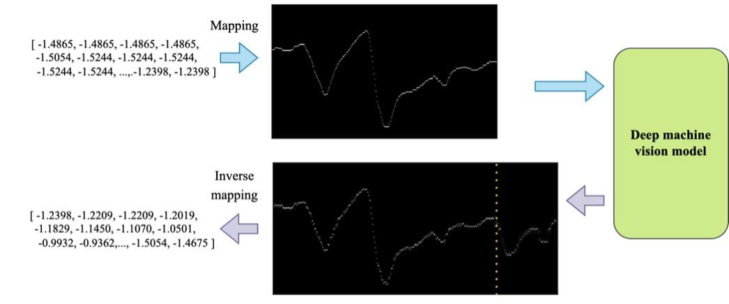
Figure 2: The overall framework of the proposed MV-DTSA.

Fig. 2 depicts the overall framework of the proposed MV-DTSA, which comprises three essential steps. Firstly, the numerical time series data from the real space S are mapped to the proposed binary machine vision time series metric space V. Secondly, deep machine vision models are selected based on the requirements of the specific task and trained using the mapped training pairs on V. Lastly, if necessary, the inverse mapping is performed to translate the output of the deep model back into the real space for further analysis.

Next, we will delve into the details of the proposed binary machine vision time series metric space and the MV-DTSF model.

The time series forecasting problem is to predict the most probable length-$O$ series in the future given the past length-$I$ series, denoting as input-$I$-predict-$O$. The long-term forecasting setting is to predict the long-term future, i.e. larger $O$. As aforementioned, we have highlighted the difficulties of long-term series forecasting: handling intricate temporal patterns and breaking the bottleneck of computation efficiency and information utilization. To tackle these two challenges, we introduce the decomposition as a builtin block to the deep forecasting model and propose Autoformer as a decomposition architecture. Besides, we design the Auto-Correlation mechanism to discover the period-based dependencies and aggregate similar sub-series from underlying periods.

3.1 Binary machine vision time series metric space

Figure 3: An illustration of the mapping process from the real space to the binary machine vision time series metric space.

Firstly, we give the definition of the proposed binary machine vision time series metric space.

Definition 1: Binary machine vision time series metric space. The Binary machine vision time series metric space is defined as a group $(V,\ d)$, where $V$ is a set of elements as defined in (1) and d is the variant of the earth mover’s distance as defined in (2).

$$V=\left\{v\in R^{c\times h\times t}\middle|{\ v}_{i,j,k}\in\left\{0,1\right\},i\in[c],j\in[h],k\in[t],\sum_{j=1}^{h}{\ v}_{i,j,k}=1\right\}\ \\$$ (1)

$$d\left(v_{1},v_{2}\right)=\int_{i=1}^{c}{\int_{k=1}^{t}{\inf_{\gamma\in\prod\left(\mathbf{v}_{\mathbf{1}}^{\mathbf{i,}\mathbf{1:h,k}}\mathbf{,}\mathbf{v}_{\mathbf{2}}^{\mathbf{i,}\mathbf{1:h,k}}\right)}{\mathbb{E}_{x,y\sim\gamma}\left\|x-y\right\|_{1}}dkdi}}\ )\\$$ (2)

where c denotes the number of variates, t denotes the length of time series, and h denotes the resolution.

In addition, we introduce the mapping function $f(*)$ from the real space of numerical time series $S=\left\{s\in R^{c\times t}\middle|s_{i,k}\in R\right\}\$to V and the corresponding inverse mapping function $f^{-1}(*)$ as expressed in (3) and (4) respectively.

$$\begin{split}\boldsymbol{v}_{i,\mathbf{1:h},\boldsymbol{k}}=\boldsymbol{f}\left(s_{i,k}\right)&=\left\langle f_{1}\left(s_{i,k}\right),f_{2}\left(s_{i,k}\right),\ldots f_{h}\left(s_{i,k}\right)\right\rangle\\ \quad f_{j}\left(s_{i,k}\right)&=\begin{cases}1,&s_{i,k}\geq MS,j=h\\ 1,&s_{i,k}\leq MS,j=1\\ 1,&j=\left\lfloor\begin{array}[]{ll}\frac{s_{i,k}+MS}{2MS}\end{array}\right\rfloor,j\in[h]\\ 0,&\text{ else }\end{cases}\end{split}$$ (3)

$$s_{i,k}=f^{-1}(\mathbf{v}_{\mathbf{i}\mathbf{,1:h,}\mathbf{k}})=\sum_{j=1}^{h}{((j-0.5)\times\frac{2MS}{h}-MS)\times v_{i,j,k}}\ \\$$ (4)

where $MS>0$ denotes the maximum scale hyperparameter. Typically, before mapping, numerical time series in real space S undergo zero-score normalization. After mapping to the binary machine vision time series metric space V, only the spatial-temporal tendency of the original time series is preserved. An illustration of the mapping function from S to V is provided in Fig. 3, where MS=1 and h=10. It is observable that, after mapping, the original time series are converted to a one-channel binary image. Meanwhile, it is evident that there exists system measurement error (SME) in the mapping and the inverse mapping process, which is formalized by Theorem 1.

Assumption 1

: After zero-score normalization, $S\sim N(\mathbf{0,I})$.

Theorem 1

: Let $\widehat{s}\in S$, the SME is defined as $\left\|f^{-1}\left(\mathbf{f}\left(\widehat{s}\right)\right)-\widehat{s}\right\|_{1}\$then the expectation of SME can be bounded as:

$$\begin{split}&\mathbb{E}\left\|f^{-1}\left(\mathbf{f}\left(\widehat{s}\right)\right)-\widehat{s}\right\|_{1}\leq g(h,MS)\\ &=ct\left(MS\left(\frac{1}{h}(\Phi(MS)-\Phi(-MS))-2+2\Phi(MS)\right)+\sqrt{\frac{2}{\pi}}e^{\frac{-MS^{2}}{2}}\right)\end{split}$$ (5)

where $\Phi$ denotes the cumulative density function of $N(\mathbf{0,I})$ and $P(*)$ denotes the probability density function of $N(0,1)$.

Denote $MS\left(\frac{1}{h}(\Phi(MS)-\Phi(-MS))-2+2\Phi(MS)\right)+\sqrt{\frac{2}{\pi}}e^{\frac{-MS^{2}}{2}}$ in (5) as the upper bound of SME. It is clear that when the MS is fixed, the upper bound of SME will decrease with the increase of the h. Then we have Proposition 1 to guarantee the convergence.

Proposition 1

: When $h\longrightarrow+\infty$, $\forall\varepsilon>0,\ \exists\delta,\ \forall MS\in R^{+}$and$\ \forall MS\geq\delta$, (6) holds.

$$\left|MS\left(\frac{1}{h}\left(\Phi(MS)-\Phi(-MS)\right)-2+2\Phi(MS)\right)+\sqrt{\frac{2}{\pi}}e^{\frac{-MS^{2}}{2}}\right|\leq\varepsilon\ \\$$ (6)

Proposition 1 guarantees the convergence of the upper bound of the SME. Specifically, if an adequate amount of GPU memory is available to specify a sufficiently large h, then SME will converge to 0 given a large enough value of MS. In practice, however, a large value of h results in a larger tensor size within the binary machine vision time series metric space, which can lead to an increase in computational load. Consequently, the selection of h should be carefully chosen to ensure computational feasibility. Then we have Proposition 2.

Proposition 2

: Given h, there always exists a best $MS^{*}$ satisfied (6) to the minimize upper bound of SME.

$$\frac{1}{h}\left(\Phi\left(MS^{*}\right)-\Phi\left(-MS^{*}\right)\right)-2+2\Phi\left(MS^{*}\right)+\frac{MS^{*}}{h}\frac{\sqrt{2}}{\sqrt{\pi}}e^{-\frac{{MS^{*}}^{2}}{2}}=0\$$ (7)

Finding an analytic solution for equation (7) is challenging. As a result, numerical solutions are typically employed in practice. Table 1 presents the numerical results of the optimal MS obtained for various h values.

Table 1: The numerical results of the optimal and the corresponding upper bound of SME given different h.

h	Best MS	Upper bound of SME
50	2.29	0.052
100	2.55	0.028
200	2.79	0.015
400	3.02	0.008
800	3.22	0.004

3.2 Machine vision assist deep time series forecasting

3.2.1 The overall architecture of the proposed MV-DTSF.

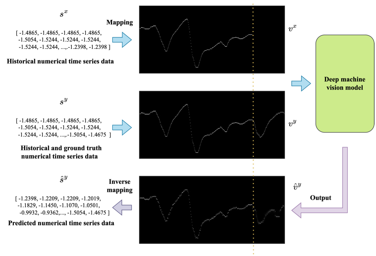
Figure 4: The architecture of the proposed MV-DTSF.

To evaluate the effectiveness of the proposed MV-DTSA framework, we apply it to TSF task. The overall architecture of the proposed MV-DTSF is depicted in Fig. 4. Initially, the historical numerical time series data, $\mathbf{s}^{\mathbf{x}}$, and the ground truth numerical time series data, $\mathbf{s}^{\mathbf{y}}$, are mapped into the binary machine vision time series metric space, V, as outlined in equation (8).

$$\begin{matrix}\mathbf{v}^{\mathbf{x}}=\mathbf{f}\left(\mathbf{s}^{\mathbf{x}}\right)&\mathbf{v}^{\mathbf{y}}=\mathbf{f}\left(\mathbf{s}^{\mathbf{y}}\right)\end{matrix}$$ (8)

Next, an end-to-end deep machine vision model D are adopted and trained with $\mathbf{v}^{\mathbf{x}}$ and $\mathbf{v}^{\mathbf{y}}$ to output the predicted results ${\widehat{\mathbf{v}}}^{\mathbf{y}}$:

$${\widehat{\mathbf{v}}}^{\mathbf{y}}=D\left(\mathbf{v}^{\mathbf{x}}\right)$$ (9)

The objective function of MV-DTSF is trying to minimize the distance better ${\widehat{\mathbf{v}}}^{\mathbf{y}}$ and $\mathbf{v}^{\mathbf{y}}$ as expressed in (10):

$$\theta^{*}=\underset{\theta}{\mathrm{argmin}}\ d\left({\widehat{\mathbf{v}}}^{\mathbf{y}},\mathbf{v}^{\mathbf{y}}\right)$$ (10)

where $\theta$ denotes parameters of the deep machine vision model D and d denotes the distance function defined in (2).

After training, the testing data is fed into the developed deep machine vision model and the corresponding output ${\widehat{\mathbf{v}}}^{\mathbf{y}}$ is inverse mapped to ${\widehat{\mathbf{s}}}^{\mathbf{y}}$ for further analysis:

$${\widehat{\mathbf{s}}}^{\mathbf{y}}=f^{-1}\left({\widehat{\mathbf{v}}}^{\mathbf{y}}\right)$$ (11)

Pseudocode of the training and testing process are offered in 1.

Algorithm 1 Training & testing process of the proposed MV-DTSF

1:Historical numerical time series data $\mathbf{s}^{\mathbf{x}}$, ground truth numerical time series data $\mathbf{s}^{\mathbf{y}}$, hyperparameter h.

2:Training

3:Initialize weights of the deep machine vision model D.

4:Find the best MS by solving (7)

5:$\mathbf{v}^{\mathbf{x}}\mathbf{=}\mathbf{f}\left(\mathbf{s}^{\mathbf{x}}\right)$  $\mathbf{v}^{\mathbf{y}}\mathbf{=}\mathbf{f}\left(\mathbf{s}^{\mathbf{y}}\right)$

6:for $i=1$ to $n$ do

7:     ${\widehat{\mathbf{v}}}^{\mathbf{y}}=D\left(\mathbf{v}^{\mathbf{x}}\right)$

8:     calculate the loss function based on (2) and update D

9:end for

10:Testing

11:$\mathbf{v}^{\mathbf{x}}\mathbf{=}\mathbf{f}\left(\mathbf{s}^{\mathbf{x}}\right)$

12:${\widehat{\mathbf{v}}}^{\mathbf{y}}=D\left(\mathbf{v}^{\mathbf{x}}\right)$

13:${\widehat{\mathbf{s}}}^{\mathbf{y}}\mathbf{=}f^{-1}\left({\widehat{\mathbf{v}}}^{\mathbf{y}}\right)$

14:Return $\widehat{\mathbf{s}}^{\mathbf{y}}$

3.2.2 Training details.

Deep machine vision models

To align with the proposed MV-DTSF, we consider the deep machine vision models utilized in vision segmentation task that can take an image as input and generate an output image of the same size. For this purpose, two classic image segmentation models, the U-net [5] and the DeepLabV2 [2], are selected as the deep machine vision models.

In-sequence data normalization

To meet the requirements of Assumption 1, we perform an in-sequence data normalization rather than normalizing the entire sequence, as described in (12):

$$\begin{matrix}\mathbf{s}^{\mathbf{x}}=\frac{\mathbf{s}^{\mathbf{x}}-mean\left(\mathbf{s}^{\mathbf{x}}\right)}{std\left(\mathbf{s}^{\mathbf{x}}\right)}&\mathbf{s}^{\mathbf{y}}=\frac{\mathbf{s}^{\mathbf{y}}-mean\left(\mathbf{s}^{\mathbf{x}}\right)}{std\left(\mathbf{s}^{\mathbf{x}}\right)}\\ \end{matrix}$$ (12)

where $mean(*)$ and $std(*)$ denote the arithmetic mean function and the standard deviation function.

Based on (12), it is noteworthy that the input numerical time series data $\mathbf{s}^{\mathbf{x}}$ and $\mathbf{s}^{\mathbf{y}}$ are normalized based on the arithmetic mean and standard deviation of $\mathbf{s}^{\mathbf{x}}$ rather than the whole sequence.

Channel independent

In the [11], the author found that dividing multivariate time series data into separate channels and feeding them independently to the same model backbone can improve prediction accuracy. In this paper, we adopt the same channel independent technique used in [11] to ensure a fair comparison in our proposed MV-DTSF.

4 Computational experiments

4.1 Datasets

Six popular open datasets, Electricity, Exchange rate, Traffic, Weather, ILI and ETTm2 are utilized to evaluate the effectiveness of the proposed MV-DTSF. Details of six datasets are reported in Table 2.

Table 2: Descriptions of datasets in this study

Dataset	Electricity	Exchange rate	Traffic	Weather	ILI	ETTm2
Features	321	8	862	21	7	7
Timesteps	26304	7588	17544	52696	966	69680

4.2 Benchmarks and model setup

To demonstrate the superiority of the proposed MV-DTSF method, five recent SOTA time series forecasting models are selected as the benchmarks in this paper, including Informer [16], Autoformer [14], FEDformer [17], patchTST [11] and DLinear [15]. The prediction length T is set to {24, 36, 48, 60} for the ILI dataset and {96, 192, 336, 720} for all other datasets, as reported in [14]. To ensure a fair comparison, we categorize the considered benchmarks into three groups based on the original length of the look-back window and the use of the channel independent technique. The grouping results are presented in Table 3. Furthermore, four variants of the MV-DTSF method are proposed in Table 3. For example, MV-DTSF-Unet-96 implies the use of U-net as the backbone of the deep machine vision model with a look-back window of 96, and MV-DTSF-DeeplabV2-336-CI implies the use of DeeplabV2 as the backbone of the deep machine vision model with a look-back window of 336 and the adoption of the channel independent technology. To alleviate the computational burden, we only consider DeeplabV2 as the backbone in group 2 and 3. Finally, we set h of all MV-DTSF models to 200 due to computational resource limitations.

Table 3: Descriptions of datasets in this study

Methods	Group	Look-back window	Channel independent
FEDformer	1	96 (36)*	×
Autoformer	1	96 (36)*	×
Informer	1	96 (36)*	×
PatchTST/42	2	336 (104)*	$\surd$
DLinear	2	336 (104)*	$\surd$
PatchTST/64	3	512 (104)*	$\surd$
MV-DTSF-Unet-96	1	96 (36)*	×
MV-DTSF-DeeplabV2-96	1	96 (36)*	×
MV-DTSF-DeeplabV2-336-CI	2	336 (104)*	$\surd$
MV-DTSF-DeeplabV2-512-CI	3	512	$\surd$

• *Look-back window for ILI dataset.

4.3 Computational results

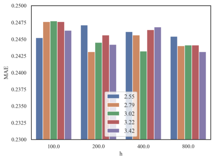
Figure 5: Forecasting performance (MAE, prediction length=96) with varying MS on dataset ETTm2 of model MV-DTSF-DeeplabV2-336-CI.

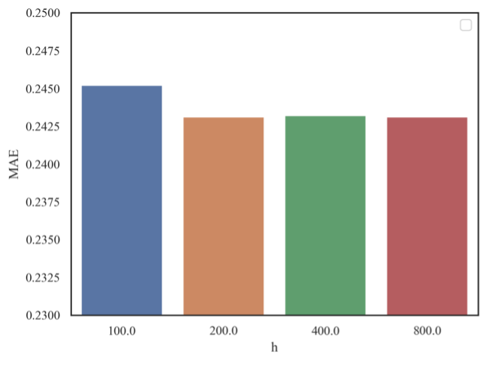
Figure 6: Forecasting performance (MAE, prediction length=96) with varying h on dataset ETTm2 of model MV-DTSF-DeeplabV2-336-CI

Fig. 5 displays the prediction performance of the MV-DTSF-DeeplabV2-336-CI model with different values of h on dataset ETTm2 for varying MS. It is observable that the best MS results align closely with the theoretical results reported in Table 3. Fig. 6 illustrates the prediction performance of the MV-DTSF-DeeplabV2-336-CI with different h on dataset ETTm2. It is apparent that increasing the value of h leads to a decrease in prediction error, which supports Proposition 1 and further demonstrates the effectiveness of the proposed MV-DTSA framework. Notably, based on the observations made from Figs 5-6, our results suggest that for large values of h, such as 800, the error between the theoretical analysis and the observed forecasting performance appears to be enlarged. This may be attributed to the sparsity of input data, which causes the deep model to fail in fitting the data effectively.

Table 4: The forecasting performance of considered methods of group 1. The best results are in bold and the second best are underlined.

Method		MV-DTSF -Unet-96		MV-DTSF -DeeplabV2-96		FEDformer-f*		FEDformer-w*		Autoformer*		Informer*
Metric		MSE	MAE	MSE	MAE	MSE	MAE	MSE	MAE	MSE	MAE	MSE	MAE
Electricity	96	NAN		0.167	0.265	0.193	0.308	0.183	0.297	0.201	0.317	0.274	0.368
	192			0.180	0.276	0.201	0.315	0.195	0.308	0.222	0.334	0.296	0.386
	336			0.190	0.286	0.214	0.329	0.212	0.313	0.231	0.338	0.300	0.364
	720			0.220	0.310	0.246	0.355	0.231	0.343	0.254	0.361	0.373	0.439
Exchange	96	0.108	0.229	0.112	0.237	0.148	0.278	0.139	0.276	0.197	0.323	0.847	0.752
	192	0.207	0.319	0.198	0.321	0.271	0.380	0.256	0.369	0.300	0.369	1.204	0.895
	336	0.304	0.407	0.358	0.434	0.460	0.500	0.426	0.464	0.509	0.524	1.672	1.036
	720	0.924	0.729	0.913	0.723	1.195	0.841	1.090	0.800	1.145	0.941	2.478	1.310
Traffic	96	NAN		0.623	0.311	0.587	0.366	0.562	0.349	0.613	0.388	0.719	0.391
	192			0.637	0.322	0.604	0.373	0.562	0.346	0.616	0.382	0.696	0.379
	336			0.652	0.327	0.621	0.383	0.570	0.323	0.622	0.337	0.777	0.420
	720			0.689	0.345	0.626	0.382	0.596	0.368	0.660	0.408	0.864	0.472
Weather	96	0.167	0.205	0.167	0.205	0.217	0.296	0.227	0.304	0.266	0.336	0.300	0.384
	192	0.238	0.271	0.217	0.252	0.276	0.336	0.295	0.363	0.307	0.367	0.598	0.544
	336	0.296	0.314	0.282	0.303	0.339	0.380	0.381	0.416	0.359	0.395	0.578	0.523
	720	0.371	0.362	0.362	0.352	0.403	0.428	0.424	0.434	0.419	0.428	1.059	0.741
ILI	24	1.915	0.829	1.782	0.810	3.228	1.260	2.203	0.963	3.483	1.287	5.764	1.677
	36	1.993	0.840	2.460	0.894	2.679	1.080	2.272	0.976	3.103	1.148	4.755	1.467
	48	1.800	0.804	1.980	0.820	2.622	1.078	2.209	0.987	2.669	1.085	4.763	1.469
	60	1.406	0.752	1.537	0.791	2.857	1.157	2.545	1.061	2.770	1.125	5.264	1.564
ETTm2	96	0.189	0.262	0.182	0.258	0.203	0.287	0.204	0.288	0.255	0.339	0.365	0.453
	192	0.260	0.313	0.247	0.301	0.269	0.328	0.346	0.363	0.281	0.340	0.533	0.563
	336	0.324	0.354	0.302	0.338	0.325	0.366	0.359	0.387	0.339	0.372	1.363	0.887
	720	0.427	0.412	0.399	0.396	0.421	0.415	0.433	0.432	0.422	0.419	3.379	1.338

• * Results are from FEDformer [17].

Table 5: The forecasting performance of considered methods of group 2 and 3. The best results are in bold and the second best is underlined.

Method		MV-DTSF -DeeplabV2-512-CI		patchTST/64 *		MV-DTSF -DeeplabV2-336-CI		patchTST/42*		Dlinear*
Metric		MSE	MAE	MSE	MAE	MSE	MAE	MSE	MAE	MSE	MAE
Weather	96	0.154	0.191	0.149	0.198	0.150	0.189	0.152	0.199	0.176	0.237
	192	0.204	0.235	0.194	0.241	0.199	0.233	0.197	0.243	0.220	0.282
	336	0.269	0.285	0.245	0.282	0.256	0.276	0.249	0.283	0.265	0.319
	720	0.340	0.338	0.314	0.334	0.342	0.339	0.320	0.335	0.323	0.362
ILI	24	1.695	0.767	1.319	0.754	NAN		1.522	0.814	2.215	1.081
	36	1.675	0.776	1.579	0.870			1.430	0.834	1.963	0.963
	48	1.650	0.773	1.553	0.815			1.673	0.854	2.130	1.024
	60	1.517	0.759	1.470	0.788			1.529	0.862	2.368	1.096
ETTm2	96	0.167	0.243	0.166	0.256	0.170	0.244	0.165	0.255	0.167	0.260
	192	0.234	0.287	0.223	0.296	0.227	0.286	0.220	0.292	0.224	0.303
	336	0.287	0.326	0.274	0.329	0.281	0.321	0.278	0.329	0.281	0.342
	720	0.376	0.389	0.362	0.385	0.379	0.384	0.367	0.385	0.397	0.421

• * Results are from patchTST [11].

Table 4 and Table 5 report the forecasting performance of the methods in groups 1, 2, and 3, respectively. However, due to computational constraints, the forecasting performance of MV-DTSF-Unet-96, MV-DTSF-DeeplabV2-512-CI, and MV-DTSF-DeeplabV2-336-CI in the Electricity and Traffic datasets are not included. It is observable that our proposed MV-DTSF method outperforms all the considered benchmarks in group 1 and achieves comparable performance in groups 2 and 3. It is worth noting that the proposed method exhibits excellent performance in terms of MAE suggesting its robustness in handling anomalies. Examples of the proposed MV-DTSF's prediction results are presented in Appendix B.

5 Conclusion

In this paper, we proposed a novel framework for time series analysis, the MV-DTSA, which analyze time series data in the novel binary machine vision time series metric space. The proposed framework consisted of three steps: (1) mapping numerical time series data to the proposed binary machine vision time series metric space, (2) designing a deep machine vision model and training it with the mapped data, and (3) if needed, inverse mapping the results from the binary machine vision time series metric space to the numerical time series data space. Experimental results on TSF task demonstrated the effectiveness of the proposed MV-DTSA framework by benchmarking against SOTA TSF models.

In summary, this paper presented a novel approach for time series data analysis, i.e., analyzing time series from the machine vision perspective. The proposed method could be applied to various time series tasks beyond time series forecasting. In the further, we would like to further improve the proposed MV-DTSA framework by customizing the deep machine vision model and refining the definition of the binary machine vision time series metric space.

Appendix A Proof of Theorem and Propositions

Theorem 1

: Let $\widehat{s}\in S$, the SME is defined as $\left\|f^{-1}\left(\mathbf{f}\left(\widehat{s}\right)\right)-\widehat{s}\right\|_{1}\$then the expectation of SME can be bounded as:

$$\begin{split}&\mathbb{E}\left\|f^{-1}\left(\mathbf{f}\left(\widehat{s}\right)\right)-\widehat{s}\right\|_{1}\leq g(h,MS)\\ &=ct\left(MS\left(\frac{1}{h}(\Phi(MS)-\Phi(-MS))-2+2\Phi(MS)\right)+\sqrt{\frac{2}{\pi}}e^{\frac{-MS^{2}}{2}}\right)\end{split}$$

where $\Phi$ denotes the cumulative density function of $N(\mathbf{0,I})$ and $P(*)$ denotes the probability density function of $N(0,1)$.

Proof:

$$\mathbb{E}\left\|f^{-1}\left(\mathbf{f}\left(\widehat{s}\right)\right)-\widehat{s}\right\|_{1}=\mathbb{E}\left(\sum_{i}^{c}{\sum_{k}^{t}\left|f^{-1}\left(\mathbf{f}\left({\widehat{s}}_{i,k}\right)\right)-{\widehat{s}}_{i,k}\right|}\right)=ct\int_{-\infty}^{+\infty}{\left|f^{-1}\left(\mathbf{f}(s)\right)-s\right|P(s)d(s)}$$ (13)

Based on (3), if $s\geq MS$, we have $\left|f^{-1}\left(\mathbf{f}(s)\right)-s\right|=s-MS$ and if $s\leq-MS$, we have $\left|f^{-1}\left(\mathbf{f}(s)\right)-s\right|=-MS-s$. Thus, if $|s|\geq MS$, we have $\left|f^{-1}\left(\mathbf{f}(s)\right)-s\right|=|s|-MS$. Considering Assumption 1, we have (14):

$$\int_{-\infty}^{-MS}{\left|f^{-1}\left(\mathbf{f}(s)\right)-s\right|P(s)d(s)}+\int_{MS}^{+\infty}{\left|f^{-1}\left(\mathbf{f}(s)\right)-s\right|P(s)d(s)}=2\int_{MS}^{+\infty}{(s-MS)P(s)d(s)}$$ (14)

Based on (3) and (4) , we have (15) :

$$\int_{MS}^{MS}{\left|f^{-1}\left(\mathbf{f}(s)\right)-s\right|P(s)d(s)}\leq\int_{MS}^{MS}{\frac{MS}{h}P(s)d(s)}$$ (15)

Then:

$$\begin{split}&\int_{-\infty}^{+\infty}{\left|f^{-1}\left(\mathbf{f}(s)\right)-s\right|P(s)d(s)}=\int_{MS}^{MS}{\left|f^{-1}\left(\mathbf{f}(s)\right)-s\right|P(s)d(s)}+\int_{-\infty}^{-MS}{\left|f^{-1}\left(\mathbf{f}(s)\right)-s\right|P(s)d(s)}\\ &+\int_{MS}^{+\infty}{\left|f^{-1}\left(\mathbf{f}(s)\right)-s\right|P(s)d(s)}\leq\int_{MS}^{MS}{\frac{MS}{h}P(s)d(s)}+2\int_{MS}^{+\infty}{(s-MS)P(s)d(s)}\\ &=MS\left(\frac{1}{h}\Phi(MS)-\frac{1}{h}\Phi(-MS)\right)+2\int_{MS}^{+\infty}{sP(s)ds}-2MS\int_{MS}^{+\infty}{P(s)d(s)}\\ &=MS\left(\frac{1}{h}\Phi(MS)-\frac{1}{h}\Phi(-MS)\right)+2\int_{MS}^{+\infty}{sP(s)ds}-2MS\left(1-\Phi(MS)\right)\ \ \\ &=MS\left(\frac{1}{h}\left(\Phi(MS)-\Phi(-MS)\right)-2+2\Phi(MS)\right)+2\int_{MS}^{+\infty}{sP(s)ds}\\ &=MS\left(\frac{1}{h}\left(\Phi(MS)-\Phi(-MS)\right)-2+2\Phi(MS)\right)+\sqrt{\frac{2}{\pi}}e^{\frac{-MS^{2}}{2}}\end{split}$$ (16)

This establishes Theorem 1.

Proposition 1

: When $h\longrightarrow+\infty$, $\forall\varepsilon>0,\ \exists\delta,\ \forall MS\in R^{+}$and$\ \forall MS\geq\delta$, (6) holds.

$$\left|MS\left(\frac{1}{h}\left(\Phi(MS)-\Phi(-MS)\right)-2+2\Phi(MS)\right)+\sqrt{\frac{2}{\pi}}e^{\frac{-MS^{2}}{2}}\right|\leq\varepsilon\ \\$$

Proof:

When $h\longrightarrow+\infty$, we have:

$$\begin{split}\lim_{h\longrightarrow+\infty}\left|MS\left(\frac{1}{h}\left(\Phi(MS)-\Phi(-MS)\right)-2+2\Phi(MS)\right)+\sqrt{\frac{2}{\pi}}e^{\frac{-MS^{2}}{2}}\right|\\ =\left|MS\left(-2+2\Phi(MS)\right)+\sqrt{\frac{2}{\pi}}e^{\frac{-MS^{2}}{2}}\right|\end{split}$$ (17)

$$\begin{split}\lim_{MS\longrightarrow+\infty}\left|MS\left(-2+2\Phi(MS)\right)\right|&=\lim_{MS\longrightarrow+\infty}\left|MS\left(-2+2\Phi(MS)\right)\right|=\lim_{MS\longrightarrow+\infty}\left|\frac{{erf}{\left(\frac{MS}{\sqrt{2}}\right)\ }-1}{\frac{1}{MS}}\right|\\ &=\lim_{MS\longrightarrow+\infty}\left|-\frac{\sqrt{2}}{\sqrt{\pi}}{MS}^{2}e^{-\frac{{MS}^{2}}{2}}\right|=0\ \end{split}$$ (18)

$$\lim_{MS\longrightarrow+\infty}\left|\sqrt{\frac{2}{\pi}}e^{\frac{-MS^{2}}{2}}\right|=0$$ (19)

We have

$$\lim_{MS\longrightarrow+\infty}\left|MS\left(-2+2\Phi(MS)\right)+\sqrt{\frac{2}{\pi}}e^{\frac{-MS^{2}}{2}}\right|=0$$ (20)

This establishes Proposition 1.

Proposition 2

: Given h, there always exists a best $MS^{*}$ satisfied (6) to the minimize upper bound of SME.

$$\frac{1}{h}\left(\Phi\left(MS^{*}\right)-\Phi\left(-MS^{*}\right)\right)-2+2\Phi\left(MS^{*}\right)+\frac{MS^{*}}{h}\frac{\sqrt{2}}{\sqrt{\pi}}e^{-\frac{{MS^{*}}^{2}}{2}}=0\$$

Proof: Note the upper bound of SME as $\chi(MS,h)$, we have:

$$\frac{\partial\chi(MS,h)}{\partial MS}=\frac{1}{h}\left(\Phi(MS)-\Phi(-MS)\right)-2+2\Phi(MS)+\frac{MS}{h}\frac{\sqrt{2}}{\sqrt{\pi}}e^{-\frac{{MS}^{2}}{2}}$$ (21)

$$\frac{\partial^{2}\chi(MS,h)}{\partial^{2}MS}=\frac{\sqrt{2}}{\sqrt{\pi}}e^{-\frac{{MS}^{2}}{2}}\left(\frac{2+h-MS^{2}}{h}\right)$$ (22)

Then we have:

$$\lim_{MS\rightarrow 0}\frac{\partial\chi(MS,h)}{\partial MS}<0\ \ \ \ \ \lim_{MS\rightarrow+\infty}\frac{\partial\chi(MS,h)}{\partial MS}>0$$ (23)

Considering the second order derivative of $\chi(MS,h)$ will be greater than 0 when $MS<\sqrt{h+2}$ and then lower than 0, and the first

Appendix B Visualizations

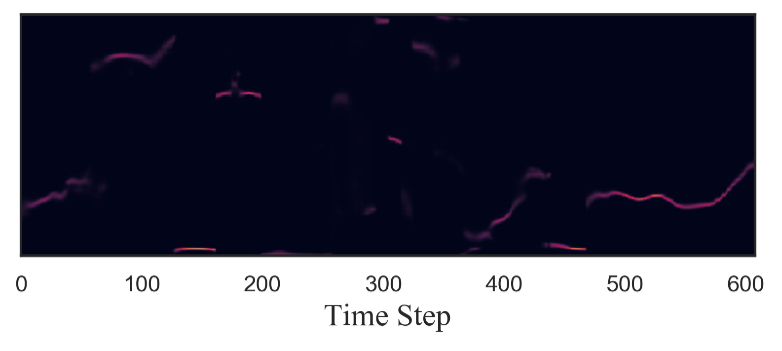
(a) Forecasting result in V

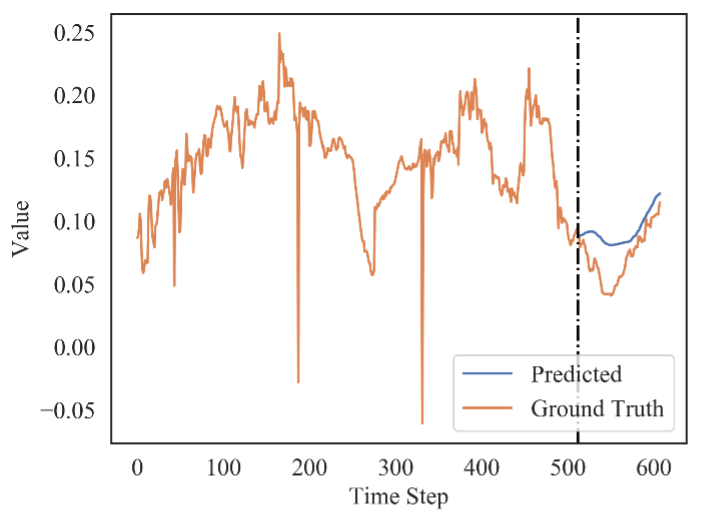
(b) Forecasting result in S

Figure 7: The forecasting results of dataset Weather (prediction length =96).

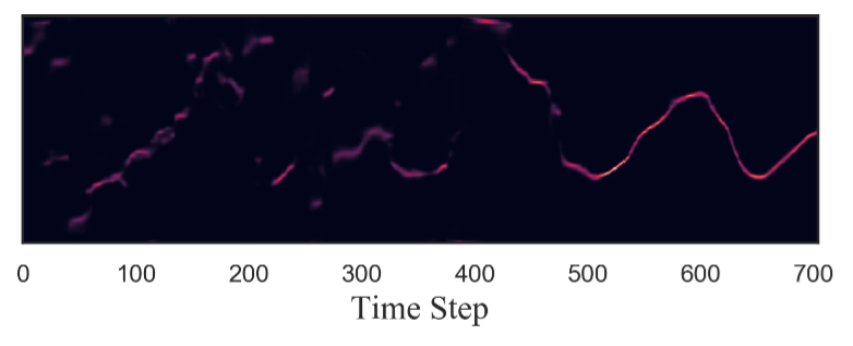
(a) Forecasting result in V

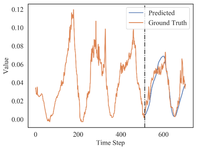
(b) Forecasting result in S

Figure 8: The forecasting results of dataset Weather (prediction length =192).

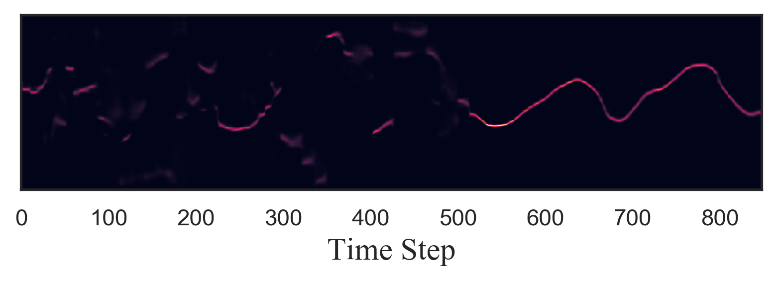
(a) Forecasting result in V

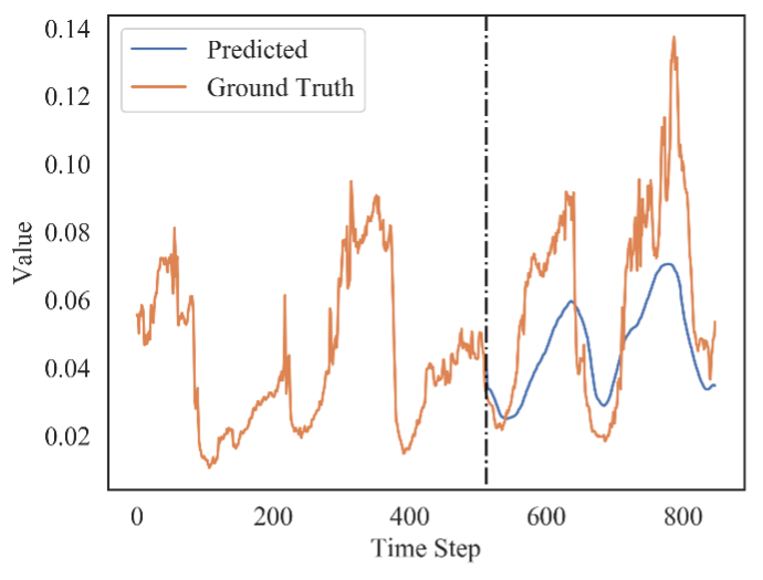
(b) Forecasting result in S

Figure 9: The forecasting results of dataset Weather (prediction length =336).

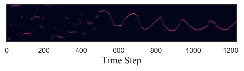
(a) Forecasting result in V

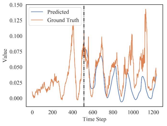
(b) Forecasting result in S

Figure 10: The forecasting results of dataset Weather (prediction length =720).

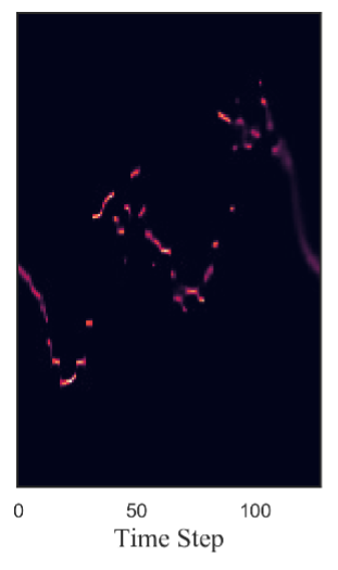
(a) Forecasting result in V

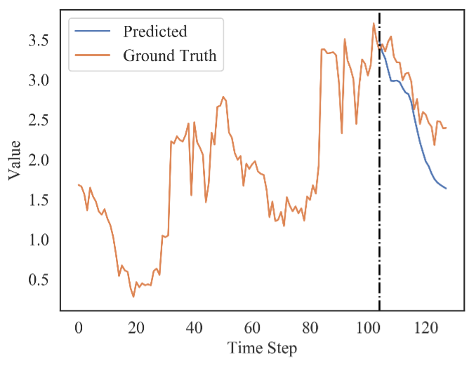
(b) Forecasting result in S

Figure 11: The forecasting results of dataset ILI (prediction length =24).

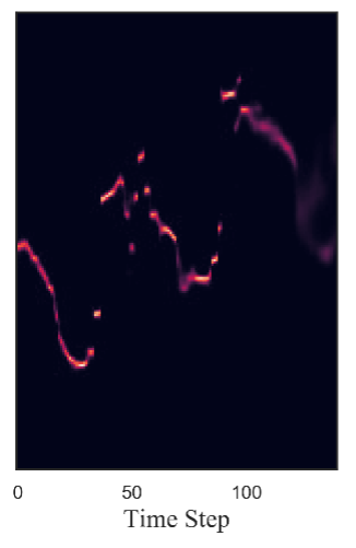
(a) Forecasting result in V

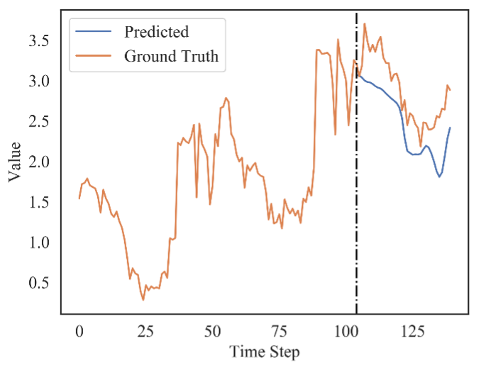
(b) Forecasting result in S

Figure 12: The forecasting results of dataset ILI (prediction length =36).

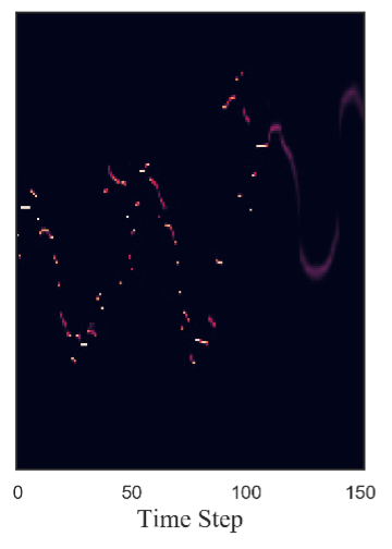
(a) Forecasting result in V

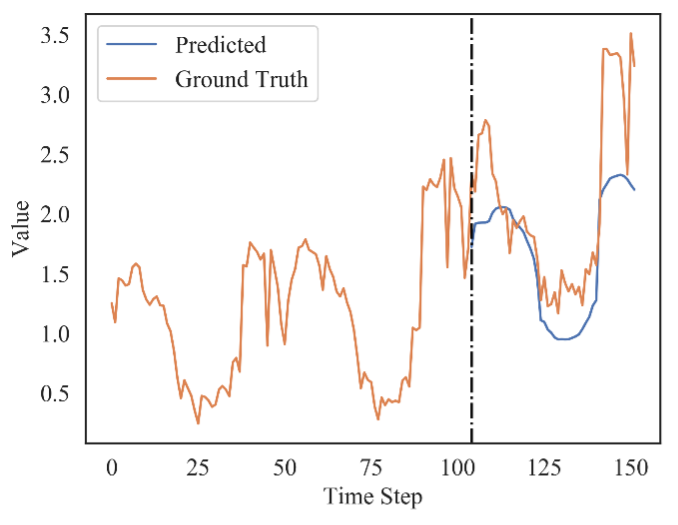
(b) Forecasting result in S

Figure 13: The forecasting results of dataset ILI (prediction length =48).

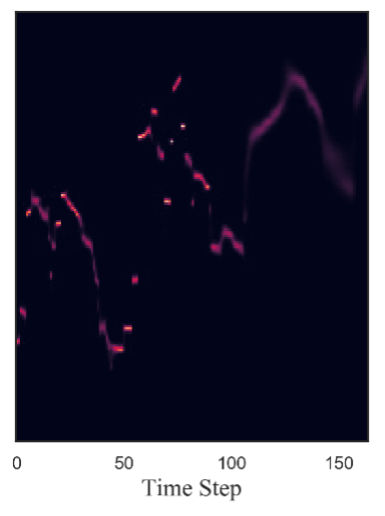
(a) Forecasting result in V

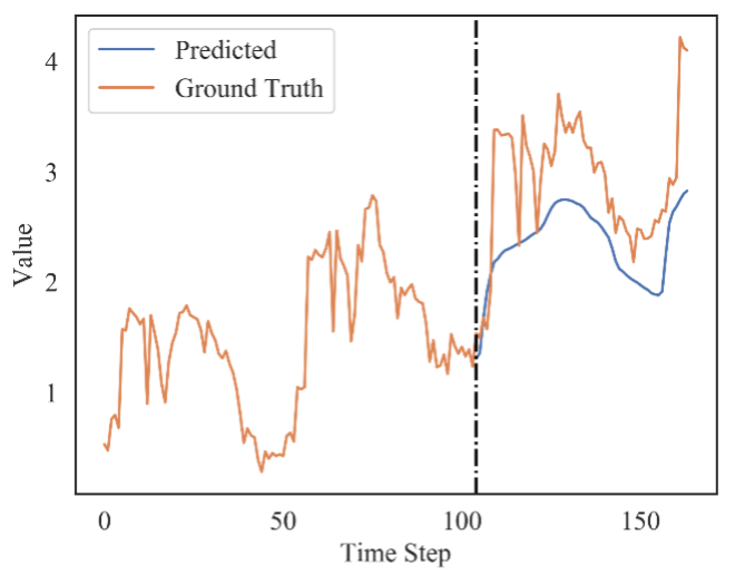
(b) Forecasting result in S

Figure 14: The forecasting results of dataset ILI (prediction length =60).

References

- [1] Shaojie Bai, J Zico Kolter, and Vladlen Koltun. An empirical evaluation of generic convolutional and recurrent networks for sequence modeling. arXiv preprint arXiv:1803.01271, 2018.
- [2] Liang-Chieh Chen, George Papandreou, Iasonas Kokkinos, Kevin Murphy, and Alan L Yuille. Deeplab: Semantic image segmentation with deep convolutional nets, atrous convolution, and fully connected crfs. IEEE transactions on pattern analysis and machine intelligence, 40(4):834–848, 2017.
- [3] Donis A Dondis. A primer of visual literacy. Mit Press, 1974.
- [4] Alexey Dosovitskiy, Lucas Beyer, Alexander Kolesnikov, Dirk Weissenborn, Xiaohua Zhai, Thomas Unterthiner, Mostafa Dehghani, Matthias Minderer, Georg Heigold, Sylvain Gelly, et al. An image is worth 16x16 words: Transformers for image recognition at scale. arXiv preprint arXiv:2010.11929, 2020.
- [5] Thorsten Falk, Dominic Mai, Robert Bensch, Özgün Çiçek, Ahmed Abdulkadir, Yassine Marrakchi, Anton Böhm, Jan Deubner, Zoe Jäckel, Katharina Seiwald, et al. U-net: deep learning for cell counting, detection, and morphometry. Nature methods, 16(1):67–70, 2019.
- [6] Rakshitha Godahewa, Kasun Bandara, Geoffrey I Webb, Slawek Smyl, and Christoph Bergmeir. Ensembles of localised models for time series forecasting. Knowledge-Based Systems, 233:107518, 2021.
- [7] James Douglas Hamilton. Time series analysis. Princeton university press, 2020.
- [8] Zhongyang Han, Jun Zhao, Henry Leung, King Fai Ma, and Wei Wang. A review of deep learning models for time series prediction. IEEE Sensors Journal, 21(6):7833–7848, 2019.
- [9] Demis Hassabis, Dharshan Kumaran, Christopher Summerfield, and Matthew Botvinick. Neuroscience-inspired artificial intelligence. Neuron, 95(2):245–258, 2017.
- [10] Yann LeCun, Yoshua Bengio, and Geoffrey Hinton. Deep learning. nature, 521(7553):436–444, 2015.
- [11] Yuqi Nie, Nam H Nguyen, Phanwadee Sinthong, and Jayant Kalagnanam. A time series is worth 64 words: Long-term forecasting with transformers. arXiv preprint arXiv:2211.14730, 2022.
- [12] Rune Pettersson. Visual information. Educational Technology, 1993.
- [13] Ashish Vaswani, Noam Shazeer, Niki Parmar, Jakob Uszkoreit, Llion Jones, Aidan N Gomez, Łukasz Kaiser, and Illia Polosukhin. Attention is all you need. Advances in neural information processing systems, 30, 2017.
- [14] Haixu Wu, Jiehui Xu, Jianmin Wang, and Mingsheng Long. Autoformer: Decomposition transformers with auto-correlation for long-term series forecasting. Advances in Neural Information Processing Systems, 34:22419–22430, 2021.
- [15] Ailing Zeng, Muxi Chen, Lei Zhang, and Qiang Xu. Are transformers effective for time series forecasting? arXiv preprint arXiv:2205.13504, 2022.
- [16] Haoyi Zhou, Shanghang Zhang, Jieqi Peng, Shuai Zhang, Jianxin Li, Hui Xiong, and Wancai Zhang. Informer: Beyond efficient transformer for long sequence time-series forecasting. In Proceedings of the AAAI conference on artificial intelligence, volume 35, pages 11106–11115, 2021.
- [17] Tian Zhou, Ziqing Ma, Qingsong Wen, Xue Wang, Liang Sun, and Rong Jin. Fedformer: Frequency enhanced decomposed transformer for long-term series forecasting. In International Conference on Machine Learning, pages 27268–27286. PMLR, 2022.