GNOT: A General Neural Operator Transformer for Operator Learning

Abstract

Learning partial differential equations’ (PDEs) solution operators is an essential problem in machine learning. However, there are several challenges for learning operators in practical applications like the irregular mesh, multiple input functions, and complexity of the PDEs’ solution. To address these challenges, we propose a general neural operator transformer (GNOT), a scalable and effective transformer-based framework for learning operators. By designing a novel heterogeneous normalized attention layer, our model is highly flexible to handle multiple input functions and irregular meshes. Besides, we introduce a geometric gating mechanism which could be viewed as a soft domain decomposition to solve the multi-scale problems. The large model capacity of the transformer architecture grants our model the possibility to scale to large datasets and practical problems. We conduct extensive experiments on multiple challenging datasets from different domains and achieve a remarkable improvement compared with alternative methods. Our code and data are publicly available at https://github.com/thu-ml/GNOT.

1 Introduction

Partial Differential Equations (PDEs) are ubiquitously used in characterizing systems in many domains like physics, chemistry, and biology (Zachmanoglou & Thoe, 1986). These PDEs are usually solved by numerical methods like the finite element method (FEM). FEM discretizes PDEs using a mesh with a large number of nodes, and it is often computationally expensive for high dimensional problems. In many important tasks in science and engineering like structural optimization, we usually need to simulate the system under different settings and parameters in a massive and repeating manner. Thus, FEM can be extremely inefficient since a single simulation using numerical methods could take from seconds to days. Recently, machine learning methods (Lu et al., 2019; Li et al., 2020, 2022b) are proposed to accelerate solving PDEs by learning an operator mapping from the input functions to the solutions of PDEs. By leveraging the expressivity of neural networks, such neural operators could be pre-trained on a dataset and then generalize to unseen inputs. The operators predict the solutions using a single forward computation, thereby greatly accelerating the process of solving PDEs. Much work has been done on investigating different neural architectures for learning operators (Hao et al., 2022). For instance, DeepONet (Lu et al., 2019) uses a branch network and a trunk network to process input functions and query coordinates. FNO (Li et al., 2020) learns the operator in the spectral space. Transformer models (Cao, 2021; Li et al., 2022b), based on attention mechanism, are proposed since they have a larger model capacity.

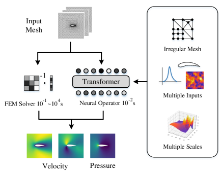
Figure 1: A pre-trained neural operator using transformers is much more efficient for the numerical simulation of physical systems. However, there are several challenges in training neural operators including irregular mesh, multiple inputs, and multiple scales.

This progress notwithstanding, operator learning for practical real-world problems is still highly challenging and the performance can be unsatisfactory. As shown in Fig. 1, there are several major challenges in current methods: irregular mesh, multiple inputs, and multi-scale problems. First, the geometric shape or the mesh of practical problems are usually highly irregular. For example, the shape of the airfoil shown in Fig. 1 is complex. However, many methods like FNO (Li et al., 2020) using Fast Fourier Transform (FFT) and U-Net (Ronneberger et al., 2015) using convolutions are limited to uniform regular grids, making it challenging to handle irregular grids. Second, the problem can rely on multiple numbers and types of input functions like boundary shape, global parameter vector or source functions. The challenge is that the model is expected to be flexible to handle different types of inputs. Third, real physical systems can be multi-scale which means that the whole domain could be divided into physically distinct subdomains (Weinan, 2011). In Fig. 1, the velocity field is much more complex near the airfoil compared with the far field. It is more difficult to learn these multi-scale functions.

Existing works attempt to develop architectures to handle these challenges. For example, Geo-FNO (Li et al., 2022a) extends FNO to irregular meshes by learning a mapping from an irregular mesh to a uniform mesh. Transformer models (Li et al., 2022b) are naturally applicable to irregular meshes. But both of them are not applicable to handle problems with multiple inputs due to the lack of a general encoder framework. Moreover, MIONet (Jin et al., 2022) uses tensor product to handle multiple input functions but it performs unsatisfactorily on multi-scale problems. To the best of our knowledge, there is no attempt that could handle these challenges simultaneously, thus limiting the practical applications of neural operators. To fill the gap, it is imperative to design a more powerful and flexible architecture for learning operators under such sophisticated scenarios.

In this paper, we propose General Neural Operator Transformer (GNOT), a scalable and flexible transformer framework for learning operators. We introduce several key components to resolve the challenges as mentioned above. First, we propose a Heterogeneous Normalized (linear) Attention (HNA) block, which provides a general encoding interface for different input functions and additional prior information. By using an aggregation of normalized multi-head cross attention, we are able to handle arbitrary input functions while keeping a linear complexity with respect to the sequence length. Second, we propose a soft gating mechanism based on mixture-of-experts (MoE) (Fedus et al., 2021). Inspired by the domain decomposition methods that are widely used to handle multi-scale problems (Jagtap & Karniadakis, 2021; Hu et al., 2022), we propose to use the geometric coordinates of input points for the gating network and we found that this could be viewed as a soft domain decomposition. Finally, we conduct extensive experiments on several benchmark datasets and complex practical problems. These problems are from multiple domains including fluids, elastic mechanics, electromagnetism, and thermology. The experimental results show that our model achieves a remarkable improvement compared with competing baselines. We reduce the prediction error by about $50\%$ compared with baselines on several practical datasets like Elasticty, Inductor2d, and Heatsink.

2 Related Work

We briefly summarize some related work on neural operators and efficient transformers.

2.1 Neural Operators

Operator learning with neural networks has attracted much attention recently. DeepONet (Lu et al., 2019) proposes a branch network and a trunk network for processing input functions and query points respectively. This architecture has been proven to approximate any nonlinear operators with a sufficiently large network. Wang et al. (2021, 2022) introduces improved architecture and training methods of DeepONets. MIONet (Jin et al., 2022) extends DeepONets to solve problems with multiple input functions. Fourier neural operator (FNO) (Li et al., 2020) is another important method with remarkable performance. FNO learns the operator in the spectral domain using the Fast Fourier Transform (FFT) which achieves a good cost-accuracy trade-off. However, it is limited to uniform grids.Several works (Li et al., 2022a; Liu et al., 2023) extend FNO to irregular grids by mapping it to a regular grid or partitioning it into subdomains. Grady II et al. (2022) combine the technique of domain decomposition (Jagtap & Karniadakis, 2021) with FNO for learning multi-scale problems. Some works also propose variants of FNO from other aspects (Gupta et al., 2021; Wen et al., 2022; Tran et al., 2021). However, these works are not scalable to handle problems with multiple types of input functions.

Another line of work proposes to use the attention mechanism for learning operators. Galerkin Transformer (Cao, 2021) proposes linear attention for efficiently learning operators. It theoretically shows that the attention mechanism could be viewed as an integral transform with a learnable kernel while FNO uses a fixed kernel. The advantage of the attention mechanism is the large model capacity and flexibility. Attention could handle arbitrary length of inputs (Prasthofer et al., 2022) and preserve the permutation equivariance (Lee, ). HT-Net (Liu et al., 2022) proposes a hierarchical transformer for learning multi-scale problems. OFormer (Li et al., 2022b) proposes an encoder-decoder architecture using galerkin-type linear attention. Transformer architecture is a flexible framework for learning operators on irregular meshes. However, its architecture still performs unsatisfactorily and has a large room to be improved when learning challenging operators with multiple inputs and scales.

2.2 Efficient Transformers

The complexity of the original attention operation is quadratic with respect to the sequence length. For operator learning problems, the sequence length could be thousands to millions. It is necessary to use an efficient attention operation. Here we introduce some existing works in CV and NLP designing transformers with efficient attention. Many works (Tay et al., 2020) paid efforts to accelerate computing attention. First, sparse and localized attention (Child et al., 2019; Liu et al., 2021; Beltagy et al., 2020; Huang et al., 2019) avoids pairwise computation by restricting windows sizes which are widely used in computer vision and natural language processing. Kitaev et al. (2020) adopt hash-based method for acceleration. Another class of methods attempts to approximate or remove the softmax function in attention. Peng et al. (2021); Choromanski et al. (2020) use the product of random features to approximate the softmax function. Katharopoulos et al. (2020) propose to replace softmax with other decomposable similarity measures. Cao (2021) propose to directly remove the softmax function. We could adjust the order of computation for this class of methods and the total complexity is linear with respect to the sequence length. Besides reducing complexity for computing attention, the mixture of experts (MoE)(Jacobs et al., 1991) are adopted in transformer architecture (Lepikhin et al., 2020; Fedus et al., 2021) to reduce computational cost while keeping a large model capacity.

3 Proposed Method

We now present our method in detail.

3.1 Problem Formulation

We consider PDEs in the domain $\Omega\subset\mathbb{R}^{d}$ and the function space $\mathcal{H}$ over $\Omega$, including boundary shapes and source functions. Our goal is to learn an operator $\mathcal{G}$ from the input function space $\mathcal{A}$ to the solution space $\mathcal{H}$, i.e., $\mathcal{G}:\mathcal{A}\rightarrow\mathcal{H}$. Here the input function space $\mathcal{A}$ could contain multiple different types, like boundary shapes, source functions distributed over $\Omega$, and vector parameters of the systems. More formally, $\mathcal{A}$ could be represented as $\mathcal{A}=\mathcal{H}\times\cdots\times\mathcal{H}\times\mathbb{R}^{p}$. For $\forall a=(a^{1}(\cdot),\ldots,a^{m}(\cdot),\theta)\in\mathcal{A}$, $a^{j}(\cdot)\in\mathcal{H}$ represents boundary shapes and source functions, and $\theta\in\mathbb{R}^{p}$ represents parameters of the system, and $\mathcal{G}(a)=u\in\mathcal{H}$ is the solution function over $\Omega$.

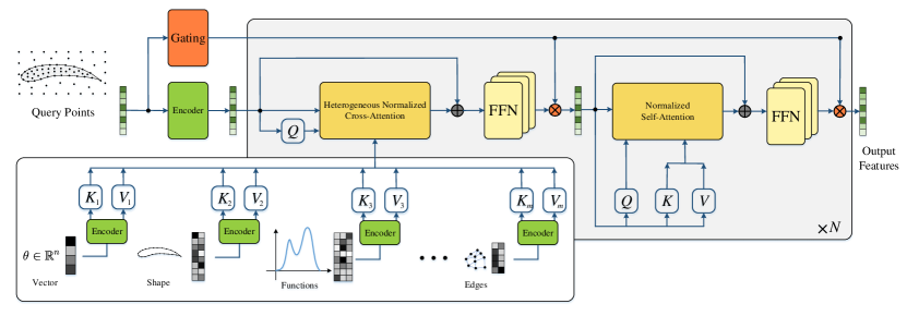
Figure 2: Overview of the model architecture. First, we encode input query points and input functions with different MLPs. Then we update features of query points using a heterogenous normalized cross-attention layer and a normalized self-attention layer. We use a gate network using geometric coordinates of query points to compute a weighted average of multiple expert FFNs. We output the features after processing them using $N$ layers of the attention block.

For learning a neural operator, we train our model with a dataset $\mathcal{D}=\{(a_{k},u_{k})\}_{1\leqslant k\leqslant D}$, where $u_{k}=\mathcal{G}(a_{k})$. In practice, since it is difficult to represent the function directly, we discretize the input functions and the solution function on irregular discretized meshes over the domain $\Omega$ using some mesh generation algorithm (Owen, 1998). For an input function $a_{k}$, we discretize it on the mesh $\{x_{i}^{j}\in\Omega\}_{1\leqslant i\leqslant N_{j}}^{1\leqslant j\leqslant m}$ and the discretized $a_{k}^{j}$ is $\{(x_{i}^{j},a^{i,j}_{k})\}_{1\leqslant i\leqslant N_{j}}$, where $a^{i,j}_{k}=a^{j}_{k}(x_{i}^{j})$. In this way, we use $\mathcal{A}_{k}=\{(x_{i}^{j},a^{i,j}_{k})\}_{1\leqslant i\leqslant N_{j}}^{1\leqslant j\leqslant m}\cup\theta_{k}$ to represent the input functions $a_{k}$.

For the solution function $u_{k}$, we discretize it on mesh $\{y_{i}\in\Omega\}_{1\leqslant i\leqslant N^{\prime}}$ and the discretized $u_{k}$ is $\{(y_{i},u^{i}_{k})\}_{1\leqslant i\leqslant N^{\prime}}$, here $u^{i}_{k}=u_{k}(y_{i})$. For modeling this operator $\mathcal{G}$, we use a parameterized neural network $\tilde{\mathcal{G}}_{w}$, which receives the input $\mathcal{A}_{k}(k=1,...,D)$ and outputs $\tilde{\mathcal{G}}_{w}(\mathcal{A}_{k})=\{\tilde{u}_{k}^{i}\}_{1\leqslant i\leqslant N^{\prime}}$ to approximate $u_{k}$. Our goal is to minimize the mean squared error(MSE) loss between the prediction and data as

$$\min_{w\in W}\frac{1}{D}\sum_{k=1}^{D}\frac{1}{N^{\prime}}\|\tilde{\mathcal{G}}_{w}(\mathcal{A}_{k})-\{u_{k}^{i}\}_{1\leqslant i\leqslant N^{\prime}}\|_{2}^{2},$$ (1)

where $w$ is a set of the network parameters and $W$ is the parameter space.

3.2 Overview of Model Architecture

Here we present an overview of our model General Neural Operator Transformer (GNOT). Transformers are a popular architecture to learn operators due to their ability to handle irregular mesh and strong expressivity. Transformers embed the input mesh points into queries $Q$, keys $K$, and values $V$ using MLPs and compute their attention. However, attention computation still has many limitations due to several challenges.

First, as the problem might have multiple different (types) input functions in practical cases, the model needs to be flexible and efficient to take arbitrary numbers of input functions defined on different meshes with different numerical scales. To obtain this goal, we first design a general input encoding protocol and embed different input functions and other available prior information using MLPs as shown in Fig 2. Then we use a novel attention block comprising a cross-attention layer followed by a self-attention layer to process these embeddings. We invent a Heterogeneous Normalized linear cross-Attention (HNA) layer which is able to take an arbitrary number of embeddings as input. The details of the HNA layer are stated in Sec 3.4.

Second, as practical problems might be multi-scale, it is difficult or inefficient to learn the whole solution using a single model. To handle this issue, We introduce a novel geometric gating mechanism that is inspired by the widely used domain-decomposition methods (Jagtap & Karniadakis, 2021). In particular, the domain-decomposition methods divide the whole domain into subdomains that are learned with subnetworks respectively. We use multiple FFNs in the attention block and compute a weighted average of these FFNs using a gating network as shown in Fig 2. The details of geometric gating are shown in Sec 3.5.

3.3 General Input Encoding

Now we introduce how our model is flexible to handle different types of input functions and preprocess these input features. The model takes positions of query points denoted by $\{x_{i}^{q}\}_{1\leqslant i\leqslant N_{q}}$ and input functions as input. We could use a multiple layer perceptron to map it to query embedding $X\in\mathbb{R}^{N_{q}\cdot n_{e}}$. In practice, we might encounter several different formats and shapes of input functions. Here we present the encoding protocol to process them to get the feature embedding $Y\in\mathbb{R}^{Nn_{e}}$ where $N$ could be arbitrary dimension and $n_{e}$ is the dimension of embedding. We call $Y$ the conditional embedding as it encodes information of input functions and extra information. We use  simple multiple layer perceptrons $f_{w}$ to map the following inputs to the embedding. Note we use one individual MLP for each input function so they do not share parameters.

• Parameter vector $\theta\in\mathbb{R}^{p}$: We could directly encode the parameter vector using the MLP, i.e, $Y=f_{w}(\theta)$ and $Y\in\mathbb{R}^{1\times n_{e}}$.

• Boundary shape $\{x_{i}\}_{1\leqslant i\leqslant N}$: If the solution relies on the shape of the boundary, we propose to extract all these boundary points as input function and embed the position of these points with MLP. Specifically, $Y=(f_{w}(x_{i}))_{1\leqslant i\leqslant N}\in\mathbb{R}^{Nd}$.

• Domain distributed functions $\{(x_{i},a_{i})\}_{1\leqslant i\leqslant N}$: If the input function is distributed over a domain or a mesh, we need to encode both the position of nodes and the function values, i.e. $Y=(f_{w}(x_{i},a_{i}))_{1\leqslant i\leqslant N}\in\mathbb{R}^{Nd}$.

Besides these types of input functions, we could also encode some additional prior like domain knowledge for specific problems using such a framework in a flexible manner which might improve the model performance. For example, we could encode the extra features of mesh points $\{(x_{i},z_{i})\}_{1\leqslant i\leqslant N}$ and edge information of the mesh $\{(x^{\operatorname{src}}_{i},x^{\operatorname{dst}}_{i},e_{i})\}_{1\leqslant i\leqslant N}$. The extra features could be the subdomain indicator of mesh points and the edges shows the topology structure of these mesh points. This extra information is usually generated when collecting the data by solving FEMs. We use MLPs to encode them into $Y=(f_{w}(x_{i},z_{i}))_{1\leqslant i\leqslant N}$ and $Y=(f_{w}(x_{i},z_{i}))_{1\leqslant i\leqslant N}$.

3.4 Heterogeneous Normalized Attention Block

Here we introduce the Heterogeneous Normalized Attention block. We calculate the heterogeneous normalized cross attention between features of query points $X$ and conditional embeddings $\{Y_{l}\}_{1\leqslant l\leqslant L}$. Then we apply a normalized self-attention layer to $X$. Specifically, the “heterogeneous” means that we use different MLPs to compute keys and values from different input features that ensure model capacity. Besides, we normalize the outputs of different attention outputs and use “mean” as the aggregation function to average all outputs. The normalization operation ensures numerical stability and also promotes the training process. Suppose we have three sequences called queries $\{\boldsymbol{q}_{i}\}_{1\leqslant i\leqslant N}$, keys$\{\boldsymbol{k}_{i}\}_{1\leqslant i\leqslant M}$ and values $\{\boldsymbol{v}_{i}\}_{1\leqslant i\leqslant M}$. The attention is computed as follows,

$$\boldsymbol{z}_{t}=\sum_{i}\frac{\exp(\boldsymbol{q}_{t}\cdot\boldsymbol{k}_{i}/\tau)}{\sum_{j}\exp(\boldsymbol{q}_{t}\cdot\boldsymbol{k}_{j}/\tau)}\boldsymbol{v}_{i},$$ (2)

where $\tau$ is a hyperparameter. For self-attention models, $\boldsymbol{q},\boldsymbol{k},\boldsymbol{v}$ are obtained by applying a linear transformation to input sequence $X=(\boldsymbol{x}_{i})_{1\leqslant i\leqslant N}$, i.e, $\boldsymbol{q}_{i}=W_{q}\boldsymbol{x}_{i}$, $\boldsymbol{k}_{i}=W_{k}\boldsymbol{x}_{i}$, $\boldsymbol{v}_{i}=W_{v}\boldsymbol{x}_{i}$. For cross attention models, $\boldsymbol{q}$ comes from the query sequence $X$ while keys and values come from another sequence $Y=(\boldsymbol{y}_{i})_{1\leqslant i\leqslant M}$, i.e, $\boldsymbol{q}_{i}=W_{q}\boldsymbol{x}_{i}$, $\boldsymbol{k}_{i}=W_{k}\boldsymbol{y}_{i}$, $\boldsymbol{v}_{i}=W_{v}\boldsymbol{y}_{i}$. However, the computational cost of the attention is $O(N^{2}n_{e})$ for self attention and $O(NMn_{e})$ for cross attention where $n_{e}$ is the dimension of embedding.

For problems of learning operators, data usually consists of thousands to even millions of points. The computational cost is unaffordable using vanilla attention with quadratic complexity. Here we propose a novel attention layer with a linear computational cost that could handle long sequences. We first normalize these sequences respectively,

$$\tilde{\boldsymbol{q}}_{i}=\operatorname{Softmax}(\boldsymbol{q}_{i}) = \left(\frac{e^{q_{ij}}}{\sum_{j}e^{q_{ij}}}\right)_{j=1,\ldots n_{e}},$$ (3)

$$\tilde{\boldsymbol{k}}_{i}=\operatorname{Softmax}(\boldsymbol{k}_{i}) = \left(\frac{e^{k_{ij}}}{\sum_{j}e^{k_{ij}}}\right)_{j=1,\ldots n_{e}}.$$ (4)

Then we compute the attention output without softmax using the following equation,

$$\boldsymbol{z}_{t}=\sum_{i}\frac{\tilde{\boldsymbol{q}}_{t}\cdot\tilde{\boldsymbol{k}}_{i}}{\sum_{j}\widetilde{\boldsymbol{q}_{t}}\cdot\tilde{\boldsymbol{k}}_{j}}\cdot\boldsymbol{v}_{i}.$$ (5)

We denote $\alpha_{t}=\left(\sum_{j}\tilde{\boldsymbol{q}}_{t}\cdot\tilde{\boldsymbol{k}}_{j}\right)^{-1}$ and the efficient attention could be represented by,

$$\boldsymbol{z}_{t}=\sum_{i}\alpha_{t}(\tilde{\boldsymbol{q}}_{t}\cdot\tilde{\boldsymbol{k}}_{i})\cdot\boldsymbol{v}_{i}=\alpha_{t}\tilde{\boldsymbol{q}}_{t}.\left(\sum_{i}\tilde{\boldsymbol{k}}_{i}\otimes\boldsymbol{v}_{i}\right).$$ (6)

We could compute $\sum_{i}\tilde{\boldsymbol{k}}_{i}\otimes\boldsymbol{v}_{i}$ first with a cost $O(Mn_{e}^{2})$ and then compute its multiplication with $\boldsymbol{q}$ with a cost $O(Nn_{e}^{2})$. The total cost is $O((M+N)n_{e}^{2})$ which is linear with respect to the sequence length.

In our model, we usually have multiple conditional embeddings and we need to fuse the information with query points. To this end, we design a cross attention using the normalized linear attention that is able to handle arbitrary numbers of conditional embeddings. Specifically, suppose we have $L$ conditional embeddings $\{Y_{l}\in\mathbb{R}^{N_{l}\times n_{e}}\}_{1\leqslant l\leqslant L}$ encoding the input functions and extra information. We first compute the queries $Q=(\boldsymbol{q}_{i})=XW_{q}$, keys $K_{l}=(\boldsymbol{k}_{i}^{l})=YW_{k}$ and values $V_{l}=(\boldsymbol{v}_{i}^{l})=YW_{v}$, and then normalize every $\boldsymbol{q}_{i}$ and $\boldsymbol{k}_{i}$ to be $\widetilde{\boldsymbol{q}_{i}}$ and $\tilde{\boldsymbol{k}}_{i}$. Then we compute the cross-attention as follows,

$$\boldsymbol{z}_{t} = \tilde{\boldsymbol{q}}_{t}+\frac{1}{L}\sum_{l=1}^{L}\sum_{i_{l}=1}^{N_{l}}\alpha_{t}^{l}(\tilde{\boldsymbol{q}}_{t}\cdot\tilde{\boldsymbol{k}}_{i_{l}})\boldsymbol{v}_{i_{l}},$$ (7)

$$= \tilde{\boldsymbol{q}}_{t}+\frac{1}{L}\sum_{l=1}^{L}\alpha_{t}^{l}\tilde{\boldsymbol{q}}_{t}\cdot\left(\sum_{i_{l}=1}^{N_{l}}\tilde{\boldsymbol{k}}_{i_{l}}\otimes\boldsymbol{v}_{i_{l}}\right).$$ (8)

where $\alpha_{t}^{l}=\frac{1}{\sum_{j=1}^{N_{l}}\tilde{\boldsymbol{q}}_{t}\cdot\tilde{\boldsymbol{k}}_{j}}$ is the normalization cofficient.

We see that the cross-attention aggregates all information from input functions and extra information. We also add an identity mapping as skip connection to ensure the information is not lost. The computational complexity of Eq. (8) is $O\left(\left(N+\sum_{l}N_{l}\right)n_{e}^{2}\right)$ also linear with sequence length.

After applying such a cross-attention layer, we impose the self-attention layer for query features, i.e,

$$\boldsymbol{z}_{t}^{\prime}=\sum_{i}\alpha_{t}(\tilde{\boldsymbol{q}}_{t}\cdot\tilde{\boldsymbol{k}}_{i})\cdot\boldsymbol{v}_{i},$$ (9)

where all of $\boldsymbol{q}$, $\boldsymbol{k}$ and $\boldsymbol{v}$ are computed with the embedding $\boldsymbol{z}_{t}$ as

$$\boldsymbol{q}_{t}=W_{q}\hat{\boldsymbol{z}}_{t},\boldsymbol{k}_{t}=W_{k}\hat{\boldsymbol{z}}_{t},\boldsymbol{v}_{t}=W_{v}\hat{\boldsymbol{z}}_{t}.$$ (10)

We use the cascade of a cross-attention layer and a self-attention layer as the basic block of our model. We tile multiple layers and multiple heads similar to other transformer models. The embedding $\boldsymbol{z}_{t}$ and $\boldsymbol{z}^{\prime}_{t}$ are divided into $H$ heads as $\boldsymbol{z}_{t}=\operatorname{Concat}(\boldsymbol{z}^{i}_{t})_{i=1}^{H}$ and $\boldsymbol{z^{\prime}}_{t}=\operatorname{Concat}(\boldsymbol{z^{\prime}}^{i}_{t})_{i=1}^{H}$. Each head $\boldsymbol{z}^{i}_{t}$ can be updated using Eq. (7) and Eq. (9).

3.5 Geometric Gating Mechanism

To handle multi-scale problems, we introduce our geometric gating mechanism based on mixture-of-experts (MoE) which is a common technique in transformers for improving model efficiency and capacity. We improve it to serve as a domain decomposition technique for dealing with multi-scale problems. Specifically, we design a geometric gating network that inputs the coordinates of the query points and outputs unnormalized scores $G_{i}(x)$ for averaging these expert networks. In each layer of our model, we use $K$ subnetworks for the MLP denoted by $E_{i}(\cdot)$. The update of $\boldsymbol{z}_{t}$ and $\boldsymbol{z^{\prime}}_{t}$ in the feedforward layer after Eq. (8) and Eq. (9) is replaced by the following equation when we have multiple expert networks as

$$\boldsymbol{z}_{t}\leftarrow\boldsymbol{z}_{t}+\sum_{i=1}^{K}p_{i}(x_{t})\cdot E_{i}(\boldsymbol{z}_{t}).$$ (11)

The weights for averaging the expert networks are computed as

$$p_{i}(x_{t})=\frac{\exp(G_{i}(x_{t}))}{\sum_{i=1}^{K}\exp(G_{i}(x_{t}))},$$ (12)

where the gating network $G(\cdot):\mathbb{R}^{d}\to\mathbb{R}^{K}$ takes the geometric coordinates of query points $x_{t}$ as inputs. The normalized outputs $p_{i}(x_{t})$ are the weights for averaging these experts.

The geometric gating mechanism could be viewed as a soft domain decomposition. There are several decision choices for the gating network. First, we could use a simple MLP to represent the gating network and learn its parameters end to end. Second, available prior information could be embedded into the gating network. For example, we could divide the domain into several subdomains and fix the gating network by handcraft. This is widely used in other domain decomposition methods like XPINNs when we have enough prior information about the problems. By introducing the gating module, our model could be naturally extended to handle large-scale and multi-scale problems.

4 Experiments

In this section, we conduct extensive experiments to demonstrate the effectiveness of our method on multiple challenging datasets.

4.1 Experimental Setup and Evaluation Protocol

Datasets. To conduct comprehensive experiments to show the scalability and superiority of our method, we choose several datasets from multiple domains including fluids, elastic mechanics, electromagnetism, heat conduction and so on. We briefly introduce these datasets here. Due to limited space, detailed descriptions are listed in the Appendix A. We list the challenges of these datasets in Table 1 where “A”, “B”, and “C” represent the problem has irregular mesh, has multiple input functions, and is multi-scale, respectively.

• Darcy2d (Li et al., 2020): A second order, linear, elliptic PDE defined on a unit square. The input function is the diffusion coefficient defined on the square. The goal is to predict the solution $u$ from coefficients $a$.

• NS2d (Li et al., 2020): A two-dimensional time-dependent Naiver-Stokes equation of a viscous, incompressible fluid in vorticity form on the unit torus. The goal is to predict the last few frames from the first few frames of the vorticity $u$.

• NACA (Li et al., 2022a): A transonic flow over an airfoil governed by the Euler equation. The input function is the shape of the airfoil. The goal is to predict the solution field from the input mesh describing the airfoil shape.

• Elasticity (Li et al., 2022a): A solid body syetem satisfying elastokinetics. The geometric shape is a unit square with an irregular cavity. The goal is to predict the solution field from the input mesh.

• NS2d-c: A two-dimensional steady-state fluids problem governed by Naiver-Stokes equations. The geometric shape is a rectangle with multiple cavities which is a highly complex shape. The goal is to predict the velocity field of $x$ and $y$ direction $u,v$ and the pressure field $p$ from the input mesh.

• Inductor2d: A two-dimensional inductor system satisfying the MaxWell equation. The input functions include the boundary shape and several global parameter vectors. The geometric shape of this problem is highly irregular and the problem is multi-scale so it is highly challenging. The goal is to predict the magnetic potential $A_{z}$ from these input functions.

• Heat: A multi-scale heat conduction problem. The input functions include multiple boundary shapes segmenting the domain and a domain-distributed function deciding the boundary condition. The physical properties of different subdomains vary greatly. The goal is to predict the temperature field $T$ from input functions.

• Heatsink: A 3d multi-physics example characterizing heat convection and conduction of a heatsink. The heat convection is accomplished by the airflow in the pipe. This problem is a coupling of laminar flow and heat conduction. We need to predict the velocity field and the temperature field from the input functions.

Dataset	Type		MIONet	FNO(-interp)	GK-Transformer	Geo-FNO	OFormer	Ours
	Challenge	Subset
Darcy2d	-	-	5.45e-2	1.09e-2	8.40e-3	1.09e-2	1.24e-2	1.05e-2
NS2d	-	part	–	1.56e-1	1.40e-1	1.56e-1	1.71e-1	1.38e-1
	-	full	–	8.20e-2	7.92e-2	8.20e-2	6.46e-2	4.43e-2
Elasticity	A	-	9.65e-2	5.08e-2	2.01e-2	2.20e-2	1.83e-2	8.65e-3
NS2d-c	A, C	$u$	2.74e-2	6.56e-2	1.52e-2	1.41e-2	2.33e-2	6.73e-3
		$v$	5.51e-2	1.15e-1	3.15e-2	2.98e-2	4.83e-2	1.55e-2
		$p$	2.74e-2	1.11e-2	1.59e-2	1.62e-2	2.43e-2	7.41e-3
NACA	A, C	-	1.32e-1	4.21e-2	1.61e-2	1.38e-2	1.83e-2	7.57e-3
Inductor2d	A, C	$A_{z}$	3.10e-2	–	2.56e-1	–	2.23e-2	1.21e-2
		$B_{x}$	3.49e-2	–	3.06e-2	–	2.83e-2	1.92e-2
		$B_{y}$	6.73e-2	–	4.45e-2	–	4.28e-2	3.62e-2
Heat	A, B, C	part	1.74e-1	–	–	–	–	4.13e-2
		full	1.45e-1	–	–	–	–	2.56e-2
Heatsink	A, B, C	$T$	4.67e-1	–	–	–	–	2.53e-1
		$u$	3.52e-1	–	–	–	–	1.42e-1
		$v$	3.23e-1	–	–	–	–	1.81e-1
		$w$	3.71e-1	–	–	–	–	1.88e-1

Table 1: Our main results of operator learning on several datasets from multiple areas. The types like $u,v$ are the physical quantities to predict and types like ”part“ denotes the size of the dataset. ”-“ means that the method is not able to handle this dataset. Lower scores mean better performance and the best results are bolded.

Baselines. We compare our method with several strong baselines listed below.

• MIONet (Jin et al., 2022): It extends DeepONet (Lu et al., 2019) to multiple input functions by using tensor products and multiple branch networks.

• FNO(-interp) (Li et al., 2020): FNO is an effective operator learning model by learning the mapping in spectral space. However, it is limited to regular mesh. We use basic interpolation to get a uniform grid to use FNO. However, it still has difficulty dealing with multiple input functions.

• Galerkin Transformer (Cao, 2021): Galerkin Transformer proposed an efficient linear transformer for learning operators. It introduces problem-dependent decoders like spectral regressors for regular grids.

• Geo-FNO (Li et al., 2022a): It extends FNO to irregular meshes by learning a mapping from the irregular grid to a uniform grid. The mapping could be learned end-to-end or pre-computed.

• OFormer (Li et al., 2022b): It uses the Galerkin type cross attention to compute features of query points. We slightly modify it by concatenating the different input functions to handle multiple input cases.

Evaluation Protocol and Hyperparameters. We use the mean $l_{2}$ relative error as the evaluation metric. Suppose $u_{i},u^{\prime}_{i}\in\mathbb{R}^{n}$ is the ground truth solution and the predicted solution for the $i$-th sample, and $D$ is the dataset size. The mean $l_{2}$ relative error is computed as follows,

$$\varepsilon=\frac{1}{D}\sum_{i=1}^{D}\frac{||u^{\prime}_{i}-u_{i}||_{2}}{||u_{i}||_{2}}.$$ (13)

For the hyperparameters of baselines and our methods. We choose the network width from $\{64,96,128,256\}$ and the number of layers from $2\sim 6$. We train all models with AdamW (Loshchilov & Hutter, 2017) optimizer with the cycle learning rate strategy (Smith & Topin, 2019) or the exponential decaying strategy. We train all models with 500 epochs with batch size from $\{4,8,16,32\}$. We run our experiments on $1\sim 8$ 2080 Ti GPUs.

4.2 Main Results for Operator Learning

The main experimental results for all datasets and methods are shown in Table 1. More details and hyperparameters could be found in Appendix B. Based on these results, we have the following observations.

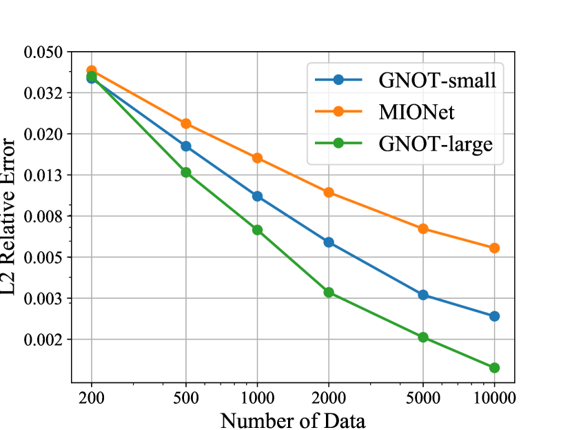
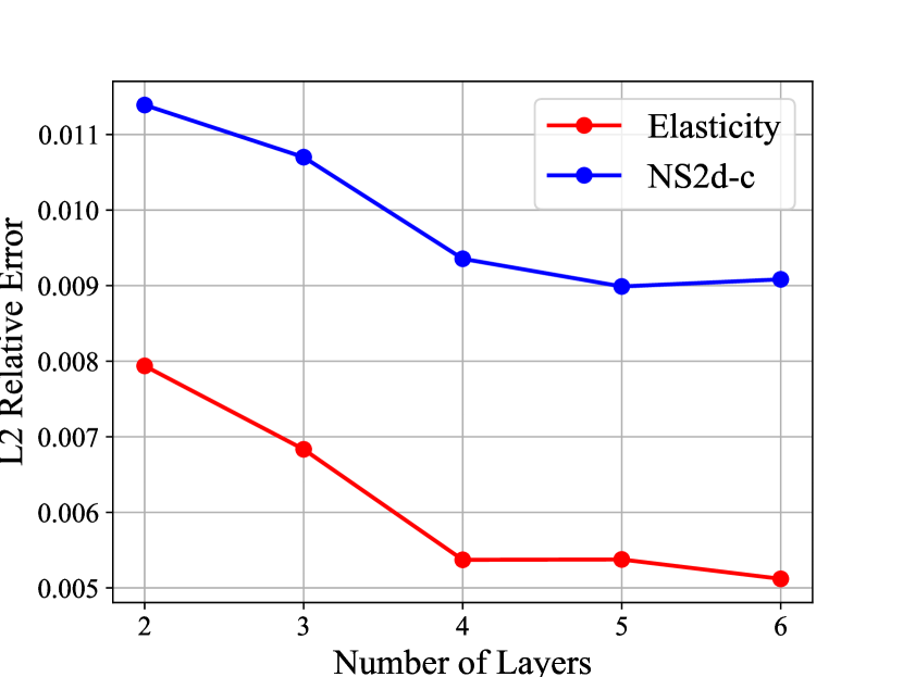
Figure 3: Results of scaling experiments for different dataset sizes (left) and different numbers of layers (right).

First, we find that our method performs significantly better on nearly all tasks compared with baselines. On datasets with irregular mesh and multiple scales like NACA, NS2d-c, and Inductor2d, our model achieves a remarkable improvement compared with all baselines. On some tasks, we reduce the prediction error by about $40\%\sim 50\%$. It demonstrates the scalability of our model. Our GNOT is also capable of learning operators on datasets with multiple inputs like Heat and Heatsink. The excellent performance on these datasets shows that our model is a general yet effective framework that could be used as a surrogate model for learning operators. This is because our heterogeneous normalized attention is highly effective to extract the complex relationship between input features. Though, GK-Transformer performs slightly better on the Darcy2d dataset which is a simple dataset with a uniform grid.

Second, we find that our model is more scalable when the amount of data increases, showing the potential to handle large datasets. On NS2d dataset, our model reduces the error over $3$ times from $13.7\%$ to $4.42\%$. On the Heat dataset, we have reduced the error from $4.13\%$ to $2.58\%$. Compared with other models like FNO(-interp), GK-Transformer on NS2d dataset, and MIONet on Heat dataset, our model has a larger capacity and is able to extract more information when more data is accessible. While OFormer also shows a good performance on the NS2d dataset, the performance still falls behind our model.

Third, we find that for all models the performance on multi-scale problems like Heatsink is worse than other datasets. This indicates that multi-scale problems are more challenging and difficult. We found that there are several failure cases, i.e. predicting the velocity distribution $u,v,w$ for the Heatsink dataset. The prediction error is very high (more than 10%). We suggest that incorporating such physical prior might help improve performance.

4.3 Scaling Experiments

One of the most important advantages of transformers is that its performance consistently gains with the growth of the number of data and model parameters. Here we conduct a scaling experiment to show how the prediction error varies when the amount of data increases. We use the NS2d-c dataset and predict the pressure field $p$. We choose MIONet as the baseline and the results are shown in Fig 3.

The left figure shows the $l_{2}$ relative error of the different models using different amounts of data. The GNOT-large denotes the model with embedding dimension 256 and GNOT-small denotes the model with embedding dimension 96. We see that all models perform better if there is more data and the relationship is nearly linear using log scale. However, the slope is different and our GNOT-large could best utilize the growing amount of data. With a larger model capacity, it is able to reach a lower error. It corresponds to the result in NLP (Kaplan et al., 2020) that the loss scales as a power law with the dataset size. Moreover, we find that our transformer architecture is more data-efficient compared with the MIONet since it has similar performance and model size with MIONet using less data.

The right figure shows how the prediction error varies with the number of layers in GNOT. Roughly we see that the error decreases with the growth of the number of layers for both Elasticity and NS2d-c datasets. The performance gain becomes small when the number of layers is more than 4 on Elasticity dataset. An efficient choice is to choose 4 layers since more layers mean more computational cost.

4.4 Ablation Experiments

We finally conduct an ablation study to show the influence of different components and hyperparameters of our model.

Necessity of different attention layers. Our attention block consists of a cross-attention layer followed by a self-attention layer. To study the necessity and the order of self-attention layers, we conduct experiments on NACA, Elasticity, and NS2d-c datasets. The results are shown in Table 2. Note that “cross$+$self” denotes a cross-attention layer followed by a self-attention layer and the rest can be done in the same manner. We find that the “cross$+$self” attention block is the best on all datasets. And the “cross$+$self” attention is significantly better than “cross$+$cross”. On the one hand, this shows that the self-attention layer is necessary for the model. On the other hand, it is a better choice to put the self-attention layer after the cross-attention layer. We conjecture that the self-attention layer after the cross-attention layer utilizes the information in both query points and input functions more effectively.

Influences of the number of experts and attention heads. We use multiple attention heads and soft mixture-of-experts containing multiple MLPs for the model. Here we study the influence of the number of experts and attention heads. We conduct this experiment on Heat which is a multi-scale dataset containing multiple subdomains. The results are shown in Table 3. The left two columns show the results of using different numbers of experts using 1 attention head. We see that using 3 experts is the best. The problem of Heat contains three different subdomains with distinct properties. It is a natural choice to use three experts so that it is easier to learn. We also find that using too many experts ($\geq 8$) deteriorates the performance. The right two columns are the results of using different numbers of attention heads with 1 expert. We find that number of attention heads has little impact on the performance. Roughly we see that using more attention heads leads to slightly better performance.

	NACA	Elasticity	NS2d-c ($p$)
cross $+$ cross	3.52e-2	3.31e-2	1.50e-2
self $+$ cross	9.53e-3	1.25e-2	9.89e-2
cross $+$ self	7.57e-3	8.65e-3	7.41e-3

Table 2: Experimental results for the necessity and order of different attention blocks.

$N_{\operatorname{experts}}$	error		$N_{\operatorname{heads}}$	error
1	0.04212		1	0.04131
3	0.03695		4	0.04180
8	0.04732		8	0.04068
16	0.04628		16	0.03952

Table 3: Results for ablation experiments on the influence of numbers of experts $N_{\mathrm{experts}}$ (left two columns) and numbers of attention heads $N_{\mathrm{heads}}$ (right two columns).

5 Conclusion

In this paper, we propose an operator learning model called General Neural Operator Transformer (GNOT). To solve the challenges of practical operator learning problems, we devise two new components, i.e. the heterogeneous normalized attention and the geometric gating mechanism. Then we conducted comprehensive experiments on multiple datasets in science and engineering. The excellent performance compared with baselines verified the effectiveness of our method. It is an attempt to use a general model architecture to handle these problems and it paves a possible direction for large-scale neural surrogate models in science and engineering.

Appendix A Details and visualization of datasets

Here we introduce more details about the datasets. For all these datasets, we generate datasets with COMSOL multi-physics 6.0. The code and datasets are publicly available at https://github.com/thu-ml/GNOT.

NS2d-c. It obeys a 2d steady-state Naiver-Stokes equation defined on a rectangle minus four circular regions, i.e. $\Omega=[0,8]^{2}\backslash\bigcup_{i=1}^{4}R_{i}$, where $R_{i}$ is a circle. The governing equation is,

$$(\boldsymbol{u}\cdot\nabla)\boldsymbol{u} = \frac{1}{\operatorname{Re}}\nabla^{2}\boldsymbol{u}-\nabla p$$ (14)

$$\nabla\cdot\boldsymbol{u} = 0$$ (15)

The velocity vanishes on boundary $\partial\Omega$, i.e. $\boldsymbol{u}=0$. On the outlet, the pressure is set to 0. On the inlet, the input velocity is $u_{x}=y(8-y)/16$. The visualization of the mesh is shown in the following Figure 4. The velocity field and pressure field is shown in Figure 5. We create 1100 samples with different positions of circles where we use 1000 for training and 100 for testing.

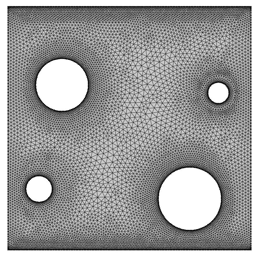
Figure 4: Visualization of mesh of the NS2d-c dataset.

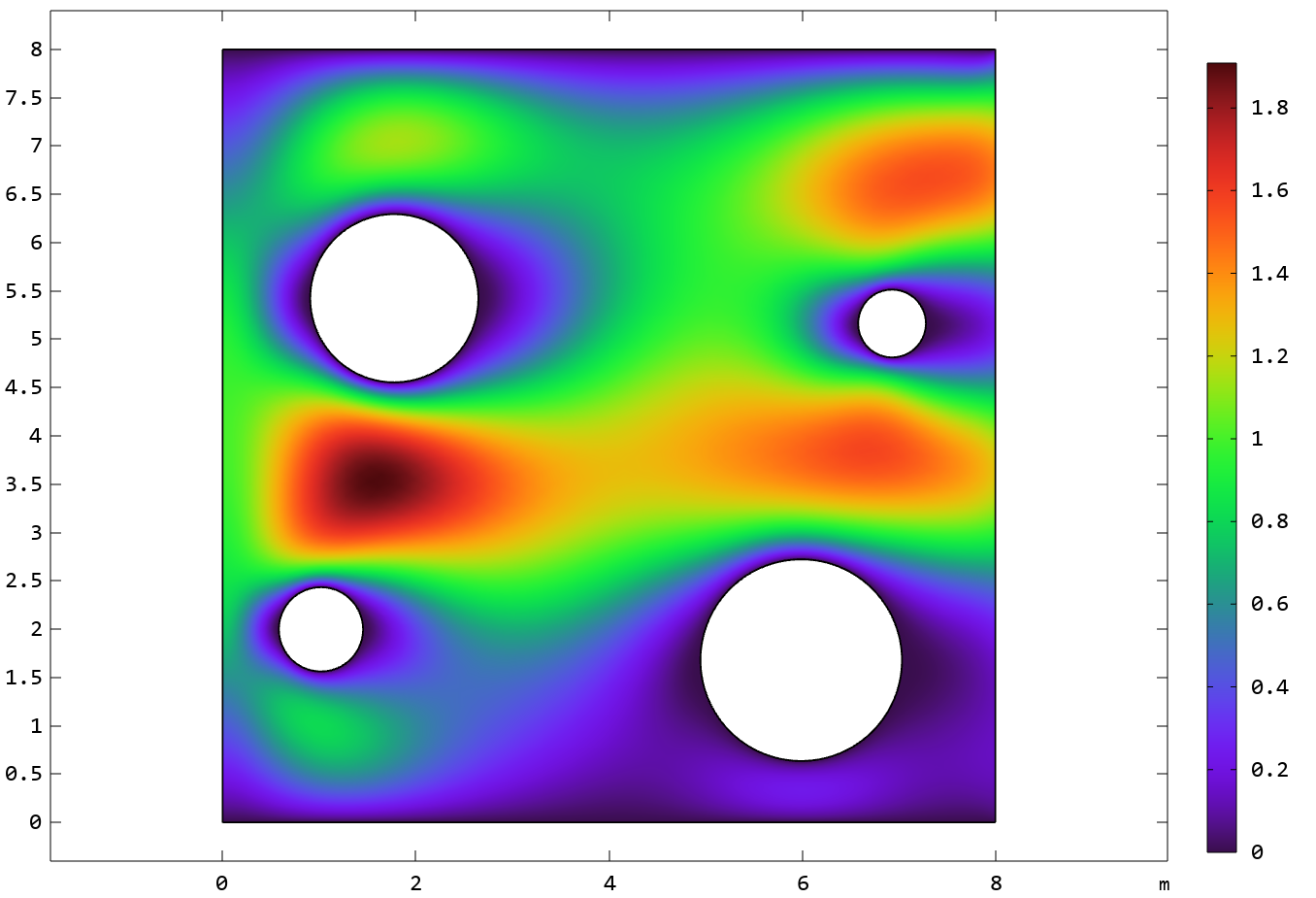
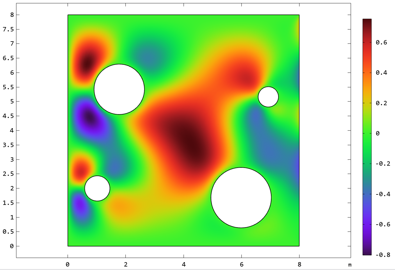
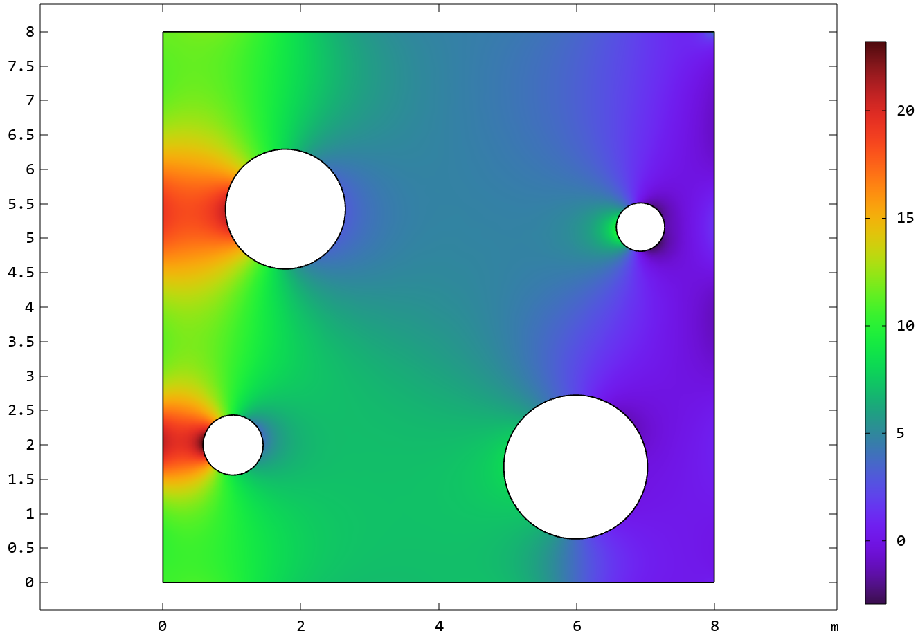
Figure 5: Visualization of velocity field $u,v$ and pressure field $p$ of NS2d-c dataset.

Inductor2d. A 2d inductor satisfying the following steady-state MaxWell’s equation,

$$\nabla\times\boldsymbol{H} = \boldsymbol{J}$$ (16)

$$\boldsymbol{B} = \nabla\times\boldsymbol{A}$$ (17)

$$\boldsymbol{J} = \sigma\boldsymbol{E}+\sigma\boldsymbol{v}\times\boldsymbol{B}+\boldsymbol{J}_{e}$$ (18)

$$\boldsymbol{B} = \mu_{0}\mu_{r}\boldsymbol{H}$$ (19)

The boundary condition is

$$\boldsymbol{n}\times\boldsymbol{A}=0$$ (20)

On the coils, the current density is,

$$\boldsymbol{J}_{e}=\frac{NI_{\operatorname{coil}}}{A}\boldsymbol{e}_{\operatorname{coil}}$$ (21)

We create 1100 inductor2d model with different geometric parameters, $I_{\operatorname{coil}}$ and material parameters $\mu_{r}$. Our goal is We use 1000 for training and 100 for testing. We plot the geometry of this problem in Figure 6. The solutions is shown in Figure 7.

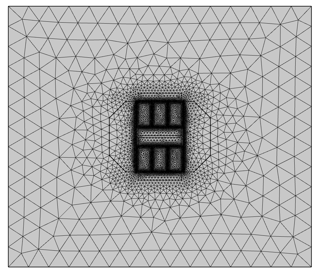
Figure 6: Visualization of mesh of the inductor2d dataset.

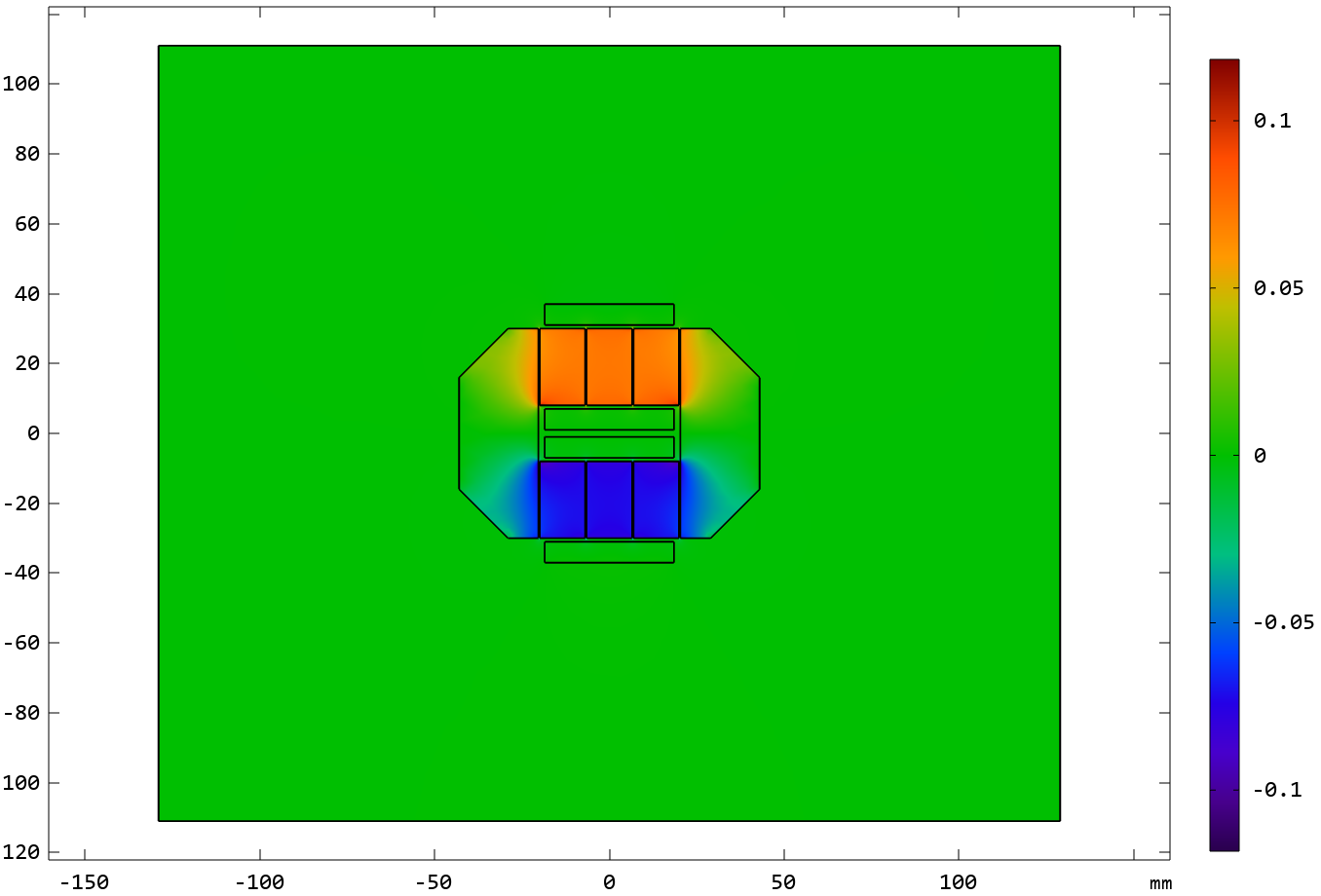
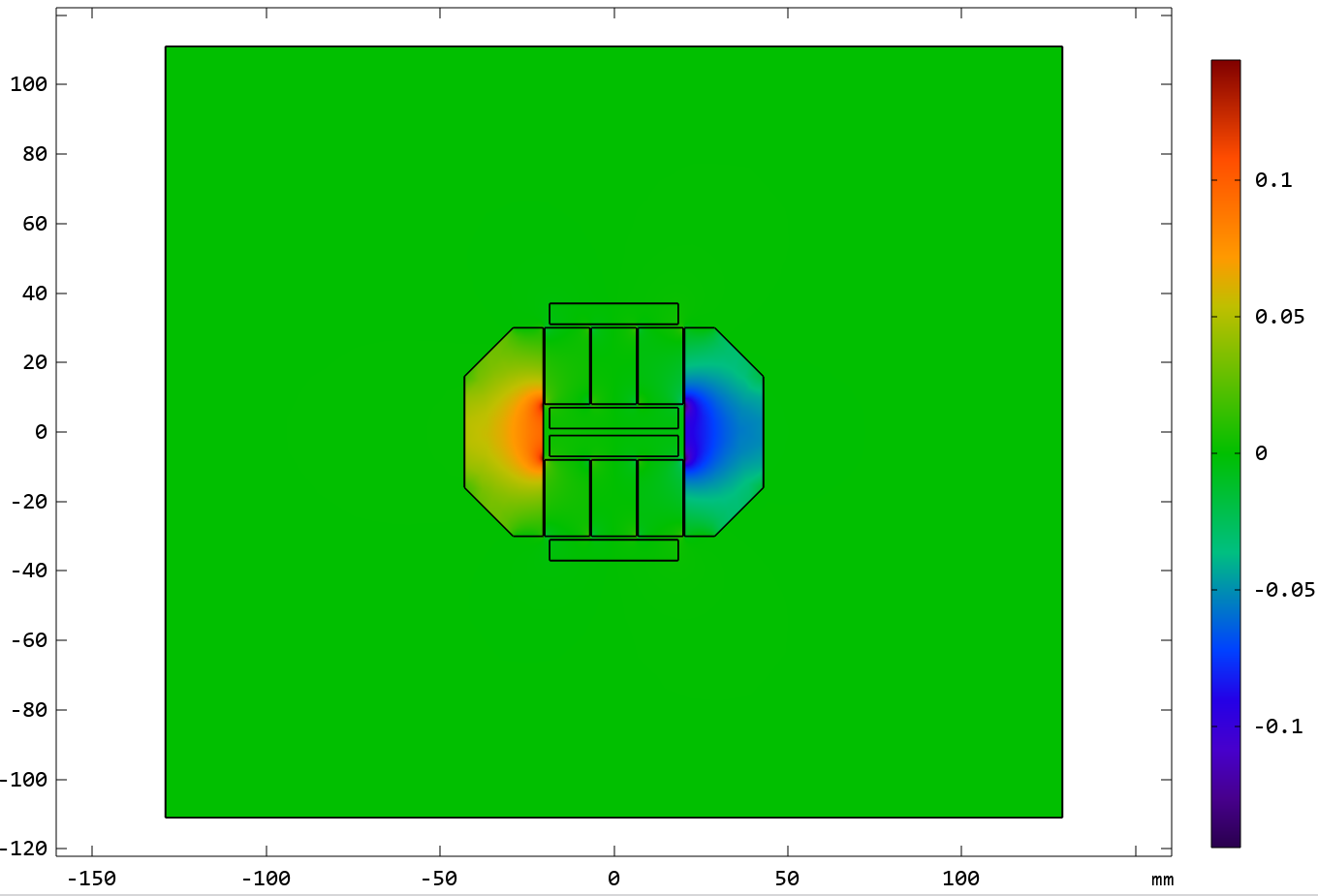
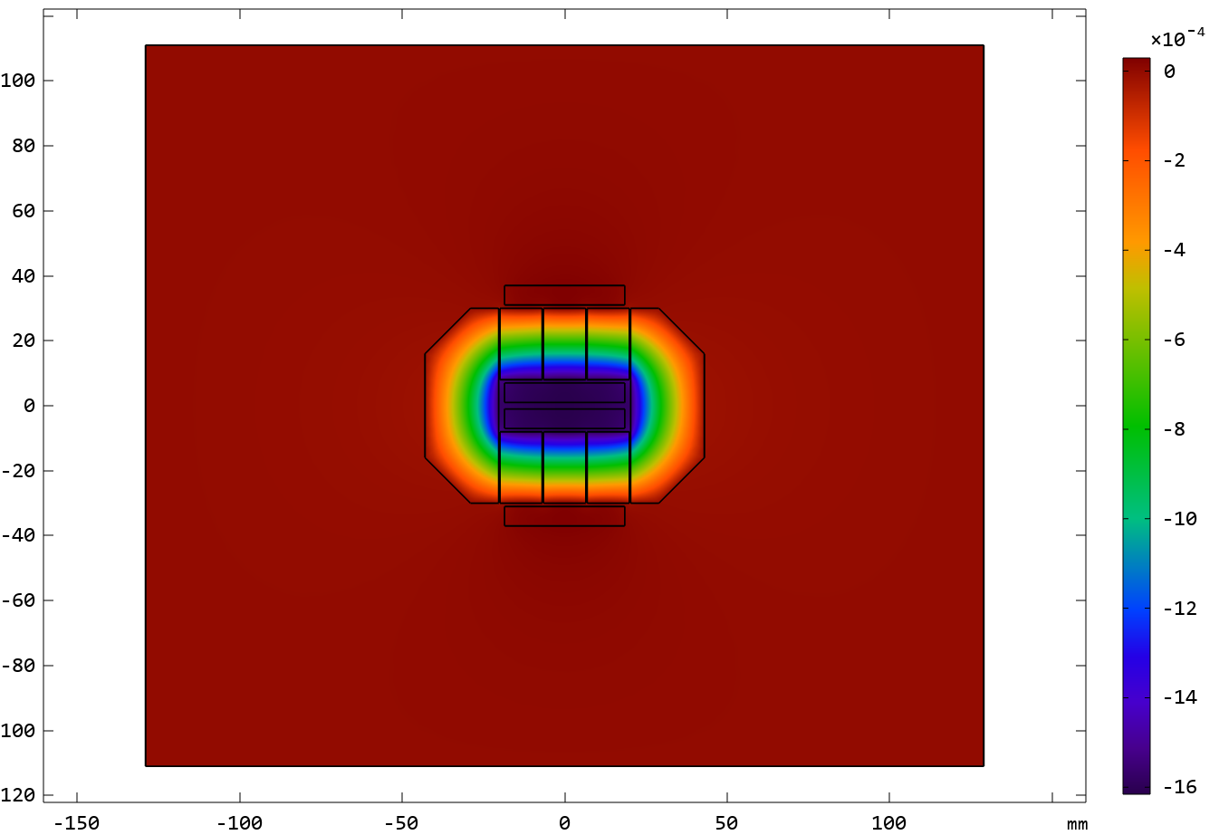
Figure 7: Visualization of $B_{x},B_{y}$ and $A_{z}$ of inductor2d dataset.

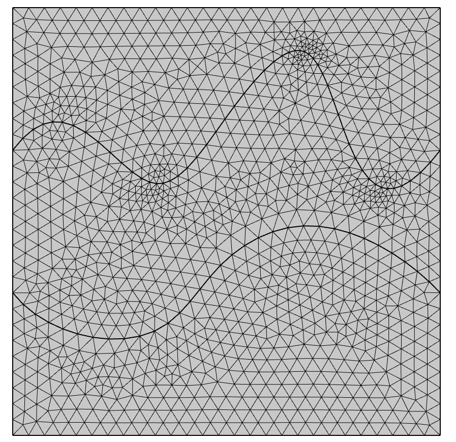
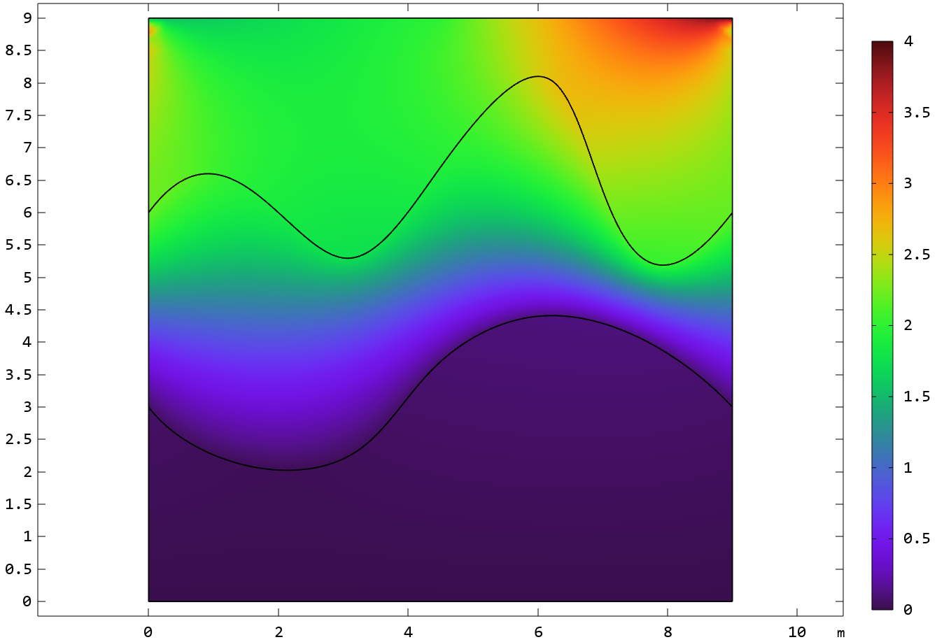
Figure 8: Left: mesh of Heat2d dataset. Right: visualization of temperature field $T$.

Heat. An example satisfying 2d steady-state heat equation,

$$\rho C_{p}\boldsymbol{u}\cdot\nabla T-k\nabla^{2}T=Q$$ (22)

The geometry is a rectangle $\Omega=[0,9]^{2}$, but it is divided into three parts using two splines. On the left and right boundary, it satisfies the periodic boundary condition. The input functions of this dataset includes the boundary temperature on the top boundary and the parameters of splines. We generate a small dataset with 1100 samples and a full datase with 5500 samples. The mesh and the temperature field is visulaized in the Figure 8.

Heatsink. A 3d steady-state multi-physics example with a coupling of heat and fluids. This example is complicated and we omit the technical details here and they could be found in the mph source files. The fluids satisfy Naiver-Stokes equation and the heat equation. The flow field and temperature field is coupled by heat convection and heat conduction. The input functions include some geometric parameters and the velocity distribution at the inlet. The goal is to predict the velocity field for the fluids and the temperature field for the whole domain. We generate 1100 samples for training and testing. The geometry of this problem is the following Figure 9. The solution fields $T,u,v,w$ are shown in Figure 10.

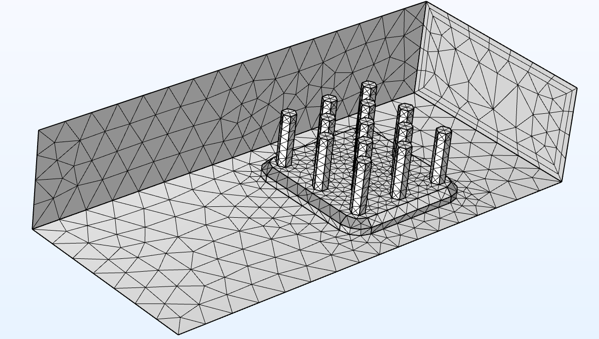
Figure 9: Visualization of mesh of the Heatsink dataset.

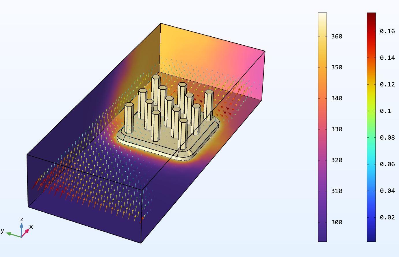
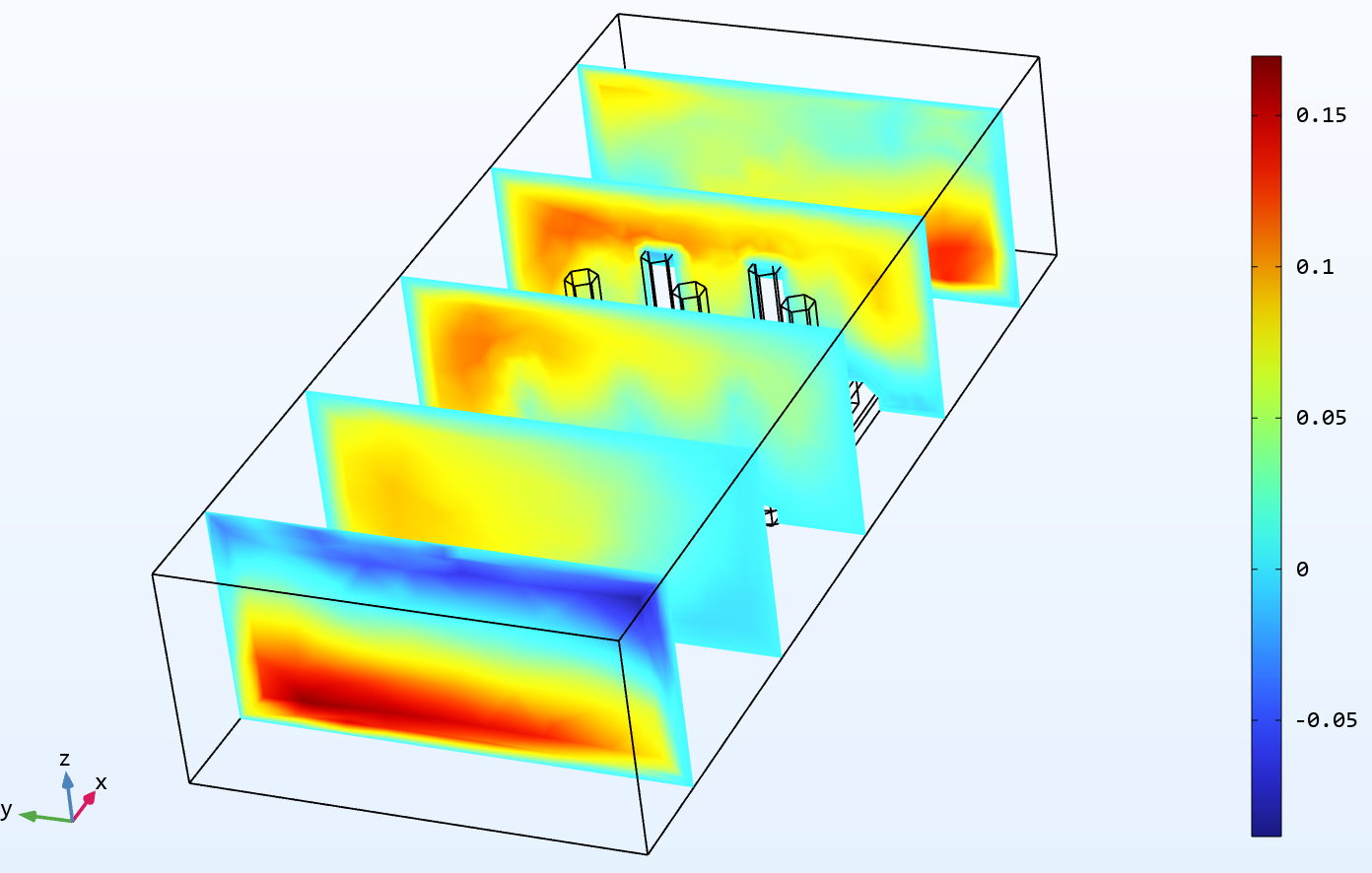
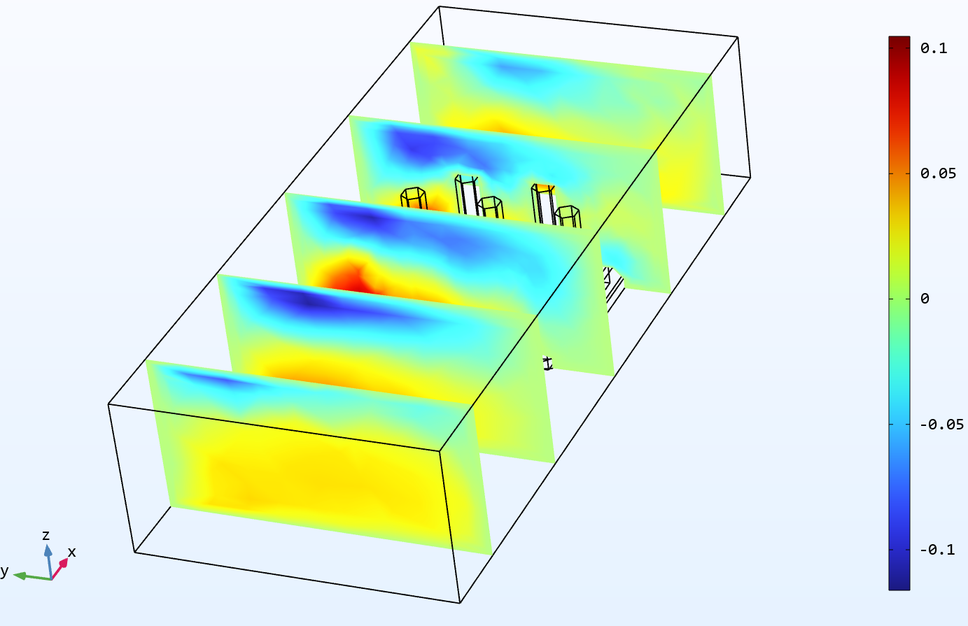
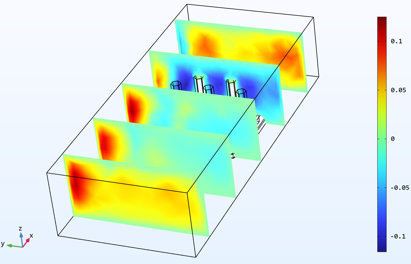
Figure 10: Visualization of $T,u,v,w$ of Heatsink dataset.

Appendix B Hyperparameters and details for models.

MIONet. We use MLPs with 4 layers and width 256 as the branch network and trunk network. When the problem has multiple input functions, the MIONet uses multiple branch networks and one trunk network. If there is only one branch, it degenerates to DeepONet. Since the discretization input functions contain different numbers of points for different samples, we pad the inputs to the maximum number of points in the whole dataset. We train MIONet with AdamW optimizer until convergence. The batch size is chosen roughly to be $4\times$ average_sequence_length.

FNO-(interp) and Geo-FNO. We use 4 FNO layers with modes from $\{12,16,32\}$ and width from $\{16,32,64\}$. The batch size is chosen from $\{8,20,32,48,64\}$. For datasets with uniform grids like Darcy2d and NS2d, we use vanilla FNO models. For datasets with irregular grids, we interpolate the dataset on a resolution from $\{80\times 80,120\times 120,160\times 160\}$. For Geo-FNO models, it degenerates to vanilla FNO models on Darcy2d and NS2d datasets. So Geo-FNO performs the same as FNO on these datasets. Other hyperparameters of Geo-FNO like width, modes, and batch size are kept the same with FNO(-interp).

GK-Transformer, OFormer, and GNOT. For all transformer models, we choose the number of heads from $\{1,4,8,16\}$. The number of layers is chosen from $\{2,3,4,5,6\}$. The dimensionality of embedding and hidden size of FFNs are chosen from $\{64,96,128,256\}$. The batch size is chosen from $\{4,8,16,20\}$. We use the AdamW optimizer with one cycle learning decay strategy. Except for NS2d and Burgers1d, we use the pointwise decoder for GK-Transformer since the spectral regressor is limited to uniform grids. Other parameters of OFormer are kept similar to its original paper. We list the details of these hyperparameters in the following table,

Hyperparameter type	Darcy2d, NS2d,Elasticity, NACA	Inductor2d, Heat,NS2d-c,NS2d-full	Heatsink
Activation function	GELU	GELU	GELU
Number of attention layers	3$\sim$4	4	4
Hidden size of attention	96	256	192
Layers of MLP	3	4	4
Hidden size of MLP	192	256	192
Hidden size of input embedding	96	128,256	96,192
Learning rate schedule	Onecycle	Onecycle	Onecycle
N experts	{1,4}	{3,4}	4
N heads	{4,8}	8	8

Table 4: Details of hyperparameters used for main experiments.

Appendix C Other Supplementary Results

We provide a runtime comparison for training our GNOT as well as baselines in the following Table 5. We see that a drawback for all transformer based methods is that training them is slower than FNO.

Time per epoch (s)	MIONet	FNO(-interp)	GK-Transformer	Geo-FNO	OFormer	GNOT
Darcy2d	18.6	13.7	27.7	13.9	29.1	29.4
NS2d	–	18.2	23.1	17.9	22.5	23.7
Elasticity	6.7	3.1	5.8	2.9	6.0	6.3
NACA	31.2	28.6	43.7	23.4	45.2	46.5
Heatsink	–	–	–	–	–	68.4

Table 5: Runtime comparison for different methods.

Appendix D Broader Impact

Learning neural operators has a wide range of real-world applications in many subjects including physics, quantum mechanics, heat engineering, fluids dynamics, and aerospace industry, etc. Our GNOT is a general and powerful model for learning neural operators and thus might accelerate the development of those fields. One of the potential negative impacts is that methods using neural networks like transformers lack theoretical guarantee and interoperability. If these unexplainable models are deployed in risk-sensitive areas, accident investigation becomes more difficult. A possible way to solve the problem is to develop more explainable and robust methods with a better theoretical guarantees or corner case protection when these models are deployed to risk-sensitive areas.

References

- Beltagy et al. (2020) Beltagy, I., Peters, M. E., and Cohan, A. Longformer: The long-document transformer. arXiv preprint arXiv:2004.05150, 2020.
- Cao (2021) Cao, S. Choose a transformer: Fourier or galerkin. Advances in Neural Information Processing Systems, 34:24924–24940, 2021.
- Child et al. (2019) Child, R., Gray, S., Radford, A., and Sutskever, I. Generating long sequences with sparse transformers. arXiv preprint arXiv:1904.10509, 2019.
- Choromanski et al. (2020) Choromanski, K., Likhosherstov, V., Dohan, D., Song, X., Gane, A., Sarlos, T., Hawkins, P., Davis, J., Mohiuddin, A., Kaiser, L., et al. Rethinking attention with performers. arXiv preprint arXiv:2009.14794, 2020.
- Fedus et al. (2021) Fedus, W., Zoph, B., and Shazeer, N. Switch transformers: Scaling to trillion parameter models with simple and efficient sparsity, 2021.
- Grady II et al. (2022) Grady II, T. J., Khan, R., Louboutin, M., Yin, Z., Witte, P. A., Chandra, R., Hewett, R. J., and Herrmann, F. J. Towards large-scale learned solvers for parametric pdes with model-parallel fourier neural operators. arXiv preprint arXiv:2204.01205, 2022.
- Gupta et al. (2021) Gupta, G., Xiao, X., and Bogdan, P. Multiwavelet-based operator learning for differential equations. Advances in Neural Information Processing Systems, 34:24048–24062, 2021.
- Hao et al. (2022) Hao, Z., Liu, S., Zhang, Y., Ying, C., Feng, Y., Su, H., and Zhu, J. Physics-informed machine learning: A survey on problems, methods and applications. arXiv preprint arXiv:2211.08064, 2022.
- Hu et al. (2022) Hu, Z., Jagtap, A. D., Karniadakis, G. E., and Kawaguchi, K. Augmented physics-informed neural networks (apinns): A gating network-based soft domain decomposition methodology. arXiv preprint arXiv:2211.08939, 2022.
- Huang et al. (2019) Huang, Z., Wang, X., Huang, L., Huang, C., Wei, Y., and Liu, W. Ccnet: Criss-cross attention for semantic segmentation. In Proceedings of the IEEE/CVF international conference on computer vision, pp. 603–612, 2019.
- Jacobs et al. (1991) Jacobs, R. A., Jordan, M. I., Nowlan, S. J., and Hinton, G. E. Adaptive mixtures of local experts. Neural computation, 3(1):79–87, 1991.
- Jagtap & Karniadakis (2021) Jagtap, A. D. and Karniadakis, G. E. Extended physics-informed neural networks (xpinns): A generalized space-time domain decomposition based deep learning framework for nonlinear partial differential equations. In AAAI Spring Symposium: MLPS, 2021.
- Jin et al. (2022) Jin, P., Meng, S., and Lu, L. Mionet: Learning multiple-input operators via tensor product. arXiv preprint arXiv:2202.06137, 2022.
- Kaplan et al. (2020) Kaplan, J., McCandlish, S., Henighan, T., Brown, T. B., Chess, B., Child, R., Gray, S., Radford, A., Wu, J., and Amodei, D. Scaling laws for neural language models. arXiv preprint arXiv:2001.08361, 2020.
- Katharopoulos et al. (2020) Katharopoulos, A., Vyas, A., Pappas, N., and Fleuret, F. Transformers are rnns: Fast autoregressive transformers with linear attention. In International Conference on Machine Learning, pp. 5156–5165. PMLR, 2020.
- Kitaev et al. (2020) Kitaev, N., Kaiser, Ł., and Levskaya, A. Reformer: The efficient transformer. arXiv preprint arXiv:2001.04451, 2020.
- (17) Lee, S. Mesh-independent operator learning for partial differential equations. In ICML 2022 2nd AI for Science Workshop.
- Lepikhin et al. (2020) Lepikhin, D., Lee, H., Xu, Y., Chen, D., Firat, O., Huang, Y., Krikun, M., Shazeer, N., and Chen, Z. Gshard: Scaling giant models with conditional computation and automatic sharding. arXiv preprint arXiv:2006.16668, 2020.
- Li et al. (2020) Li, Z., Kovachki, N., Azizzadenesheli, K., Liu, B., Bhattacharya, K., Stuart, A., and Anandkumar, A. Fourier neural operator for parametric partial differential equations. arXiv preprint arXiv:2010.08895, 2020.
- Li et al. (2022a) Li, Z., Huang, D. Z., Liu, B., and Anandkumar, A. Fourier neural operator with learned deformations for pdes on general geometries. arXiv preprint arXiv:2207.05209, 2022a.
- Li et al. (2022b) Li, Z., Meidani, K., and Farimani, A. B. Transformer for partial differential equations’ operator learning. arXiv preprint arXiv:2205.13671, 2022b.
- Liu et al. (2023) Liu, S., Hao, Z., Ying, C., Su, H., Cheng, Z., and Zhu, J. Nuno: A general framework for learning parametric pdes with non-uniform data. arXiv preprint arXiv:2305.18694, 2023.
- Liu et al. (2022) Liu, X., Xu, B., and Zhang, L. Ht-net: Hierarchical transformer based operator learning model for multiscale pdes. arXiv preprint arXiv:2210.10890, 2022.
- Liu et al. (2021) Liu, Z., Lin, Y., Cao, Y., Hu, H., Wei, Y., Zhang, Z., Lin, S., and Guo, B. Swin transformer: Hierarchical vision transformer using shifted windows. In Proceedings of the IEEE/CVF International Conference on Computer Vision, pp. 10012–10022, 2021.
- Loshchilov & Hutter (2017) Loshchilov, I. and Hutter, F. Decoupled weight decay regularization. arXiv preprint arXiv:1711.05101, 2017.
- Lu et al. (2019) Lu, L., Jin, P., and Karniadakis, G. E. Deeponet: Learning nonlinear operators for identifying differential equations based on the universal approximation theorem of operators. arXiv preprint arXiv:1910.03193, 2019.
- Owen (1998) Owen, S. J. A survey of unstructured mesh generation technology. IMR, 239:267, 1998.
- Peng et al. (2021) Peng, H., Pappas, N., Yogatama, D., Schwartz, R., Smith, N. A., and Kong, L. Random feature attention. arXiv preprint arXiv:2103.02143, 2021.
- Prasthofer et al. (2022) Prasthofer, M., De Ryck, T., and Mishra, S. Variable-input deep operator networks. arXiv preprint arXiv:2205.11404, 2022.
- Ronneberger et al. (2015) Ronneberger, O., Fischer, P., and Brox, T. U-net: Convolutional networks for biomedical image segmentation. In International Conference on Medical image computing and computer-assisted intervention, pp. 234–241. Springer, 2015.
- Smith & Topin (2019) Smith, L. N. and Topin, N. Super-convergence: Very fast training of neural networks using large learning rates. In Artificial intelligence and machine learning for multi-domain operations applications, volume 11006, pp. 369–386. SPIE, 2019.
- Tay et al. (2020) Tay, Y., Dehghani, M., Bahri, D., and Metzler, D. Efficient transformers: A survey. ACM Computing Surveys (CSUR), 2020.
- Tran et al. (2021) Tran, A., Mathews, A., Xie, L., and Ong, C. S. Factorized fourier neural operators. arXiv preprint arXiv:2111.13802, 2021.
- Wang et al. (2021) Wang, S., Wang, H., and Perdikaris, P. Learning the solution operator of parametric partial differential equations with physics-informed deeponets. Science advances, 7(40):eabi8605, 2021.
- Wang et al. (2022) Wang, S., Wang, H., and Perdikaris, P. Improved architectures and training algorithms for deep operator networks. Journal of Scientific Computing, 92(2):1–42, 2022.
- Weinan (2011) Weinan, E. Principles of multiscale modeling. Cambridge University Press, 2011.
- Wen et al. (2022) Wen, G., Li, Z., Azizzadenesheli, K., Anandkumar, A., and Benson, S. M. U-fno—an enhanced fourier neural operator-based deep-learning model for multiphase flow. Advances in Water Resources, 163:104180, 2022.
- Zachmanoglou & Thoe (1986) Zachmanoglou, E. C. and Thoe, D. W. Introduction to partial differential equations with applications. Courier Corporation, 1986.