Towards Enhanced Controllability of Diffusion Models

Abstract

Denoising Diffusion models have shown remarkable capabilities in generating realistic, high-quality and diverse images. However, the extent of controllability during generation is underexplored. Inspired by techniques based on GAN latent space for image manipulation, we train a diffusion model conditioned on two latent codes, a spatial content mask and a flattened style embedding. We rely on the inductive bias of the progressive denoising process of diffusion models to encode pose/layout information in the spatial structure mask and semantic/style information in the style code. We propose two generic sampling techniques for improving controllability. We extend composable diffusion models to allow for some dependence between conditional inputs, to improve the quality of generations while also providing control over the amount of guidance from each latent code and their joint distribution. We also propose timestep dependent weight scheduling for content and style latents to further improve the translations. We observe better controllability compared to existing methods and show that without explicit training objectives, diffusion models can be used for effective image manipulation and image translation.

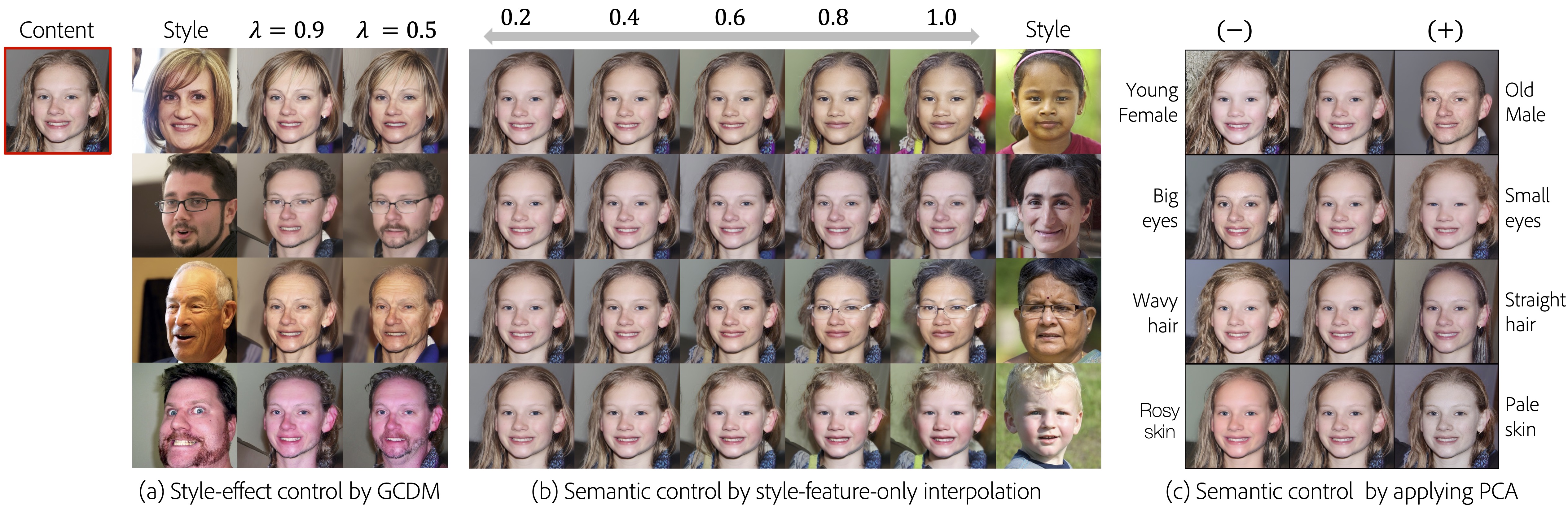
Figure 1: We train a latent diffusion model for image-to-image translation by conditioning on content and style latent spaces (Sec.3.1). We further propose inference time techniques, generalized composable sampling (Sec.3.3) and timestep scheduling (Sec.3.2) to improve controllability. Controlling $\lambda$ in our GCDM formulation results in different magnitudes of style translation in (a). While fixing the content feature, applying convex combinations between the style features from content and style images show the smooth interpolations as shown in (b). PCA on the learned style code gives disentangled attribute specific manipulation directions in (c). Detailed experiment setups and more results are provided in Sections E.1, E.2 and in Fig. 26 in the supplementary.

1 Introduction

Diffusion Models [46, 18] (DM) have gained much attention due to their impressive performance in image generation [8, 41, 42] and likelihood estimation [38]. While many efforts have concentrated on improving image generation quality [38, 45, 53] and sampling speed [47, 28, 36], relatively less attention has focused on enhancing controllability of diffusion models.

Improving editability and controllability in various other forms of generative models (e.g., GANs [14, 15, 50], VAE [27, 2] and Flow-based Models [10, 11]) has been one of the most prominent research topics in the past few years. GANs such as StyleGAN-v2 [22] have been shown to inherently learn smooth and regular latent spaces [15, 50] that enable meaningful edits and manipulations on a real or generated image. The enhanced controls are useful for many practical applications such as Image Synthesis [39], Domain Adaptation [20], Style Transfer [21, 32] and Interpretability [31] to name a few. Despite high quality and diverse image generations, it is less clear how to manipulate the latent space of diffusion models that is composed of a sequence of gradually denoised 2d samples.

An alternative to using the inherent latent space of GANs for manipulation is to learn multiple external disentangled latent spaces to condition the generation  [39, 21, 32, 29]. A common theme across such methods is to learn a structure/content code to capture the underlying structure (e.g., facial shape and pose in face images) and a texture/style code to capture global semantic information (e.g. visual appearance, color, hair style etc.). Similar approaches have been tried in diffusion models in  [30, 40], however these techniques do not learn multiple controllable latent spaces. Other inference time editing techniques such as  [16, 24, 33, 49, 34] either require computationally expensive optimization (of the conditional embeddings and/or the model) for each sample during inference or do not provide fine-grained controllability. Composable Diffusion Models [34] (CDM) proposes a way to compose multiple conditional inputs but assumes the inputs are independent, which may not always be true (Section 3.3).

In this paper, we propose a novel framework as shown in Fig. 2 to effectively learn two latent spaces to enhance controllability in diffusion models. Inspired by  [39, 29] we add a Content Encoder that learns a spatial layout mask and a Style Encoder that outputs a flattened semantic code to condition the diffusion model during training (Section 3.1). The content and style codes are injected differently into the UNet [43] to ensure they encode different semantic factors of an image.

Though decomposing content and style information from an image enables better controllability, enforcing independence between the codes may not always be ideal. For example, face structure (e.g. square or round face) that is ideally encoded in the content code and gender (e.g. male or female) an attribute encoded in the style code [39], may not be independent and treating them as such might lead to unnatural compositions (Fig. 3). Similarly, CDM [34] assumes conditioning inputs are independent and hence shows unnatural compositions for certain prompts like ‘a flower’ and ‘a bird’ (see Fig.6 in [34]). We extend the formulation in  [34] and propose Generalized Composable Diffusion Models (GCDM) to support compositions during inference when the conditional inputs are not necessarily independent (Section 3.3). This also provides the ability to control the amount of information from content, style and their joint distribution separately during sampling. We observe significantly better translations with GCDM and also show improved compositions in Stable Diffusion compared to CDM (Fig. 5).

In addition, we leverage the inductive bias [1, 5, 6] of diffusion models that learns low frequency layout information in earlier steps and high frequency or imperceptible details in the later steps of the reverse diffusion process, to further improve results. We use a predefined controllable timestep dependent weight schedule to compose the content and style codes during generation. This simulates the mixture of denoising experts proposed in [1] by virtue of varying the conditional information (instead of the entire model) at different timesteps during inference. Some examples generated using the proposed model are shown in Fig. Towards Enhanced Controllability of Diffusion Models.

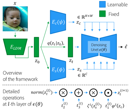
Figure 2: (Top) overview of our proposed framework. We first obtain $z_{0}$ from the pretrained Autoencoder [12], which is the actual input for the LDM [42]. The external encoders $E_{c}(\psi)$ and $E_{s}(\phi)$ and the denoising UNet $\epsilon(\theta)$ are trained together without any additional objectives. (Bottom) shows the details of injecting style and content information into the denoising UNet at the $\ell$-th layer as described in Section 3.1.

Moreover, we also show that the learned latent spaces are manipulatable. We apply PCA on the style and content latent spaces and identify meaningful attribute specific manipulation directions similar to [15] as shown in Fig. Towards Enhanced Controllability of Diffusion Models (c). We also observe that the proposed setup learns latent spaces that support smooth interpolations (Fig. Towards Enhanced Controllability of Diffusion Models (b)).

To the best of our knowledge, there is no existing work that trains diffusion models with multiple latent spaces, generalizes composable diffusion models and leverages timestep scheduling for image translation and manipulation.

2 Preliminaries and Related Works

In this section, we describe the preliminaries that our approach builds on and related works in the literature.

2.1 Diffusion Models

Diffusion Models [46] like DDPM [18] showed impressive image generation and likelihood estimation but had a computationally expensive sampling procedure. DDIM [47] reduced the sampling time by deriving a non-Markovian variant of DDPM. Similarly, ImprovedDDPM [38] also improved sampling speed and proposed to learn the variance schedule that was fixed in previous works to enhance mode coverage. DPM-solver [35] and DPM-solver++ [36] proposed high-order ODE solvers for faster sampling. DDGAN [51] combined the best of GANs and diffusion models to retain the mode coverage and quality of diffusion models while making it faster like GANs. LDM [42] used a pretrained autoencoder [12] to learn a lower capacity latent space and trained a diffusion model on the learned latent space (in contrast to pixel space in previous works), reducing time and memory complexity significantly without loss in quality. More descriptions are provided in Section C in the supplementary.

2.2 Controllability in Diffusion Models

Guidance:
Some recent works have explored modeling the conditional density $p(x_{t}|c)$ for controllability. Dhariwal et al. [8] proposed to use a pretrained classifier but finetuning a classifier that estimates gradients from noisy images, which increases the complexity of the overall process [19]. Ho et al. [19] proposed to use an implicit classifier while Composable Diffusion Models [34] (CDM) extend the classifier free guidance approach to work with multiple conditions assuming conditional independence. Though guidance approaches help control the generation, they do not offer fine grained controllability or support applications such as reference based image translation.

Conditional DMs:
Conditional Diffusion Models have been explored in diverse applications showing state–of–the–art performance in text to image generation (DALLE2 [41], Imagen [45], Parti [53]). These methods use pretrained CLIP or similar embeddings that support interpolation but not further editability. DiffAE [40] proposed to learn a semantic space that has nice properties making it suitable image manipulation. However, a single latent space capturing all the information makes it difficult to isolate attributes to manipulate.

Inference only Editing:
Several works have proposed inference-time editing techniques on top of pretrained diffusion models. SDEdit [37] enables structure preserving edits while Prompt-to-prompt [16] modifies the attention maps from cross-attention layers to add, remove or reweigh importance of an object in an image. DiffusionCLIP [25], Imagic [24] and Unitune [49] propose optimization based techniques for text based image editing. Textual Inversion [13] and DreamBooth [44] finetunes pretrained models using few reference images to get personalized models. Though the above techniques are helpful with editing, most of these methods require computationally expensive optimization, modify the weights of pretrained model for each sample, and/or doesn’t support fine–grained controllability for reference based image translation. The closest related work to ours is DiffuseIT [30]. They enabled reference and text guided image translation by leveraging Dino-VIT [3] to encode content and style. However, their approach requires costly optimization during inference and doesn’t support controlling the final generation.
Inductive Bias of Diffusion Models:
On top of the inductive bias [5, 6] of Diffusion Models, eDiffi [1] proposed to train models specialized to a subset of the timesteps to improve generations drastically. MagicMix [33] interpolates noise maps while providing different embeddings at different timesteps. Though these approaches show the advantages of the inductive bias, it hasn’t been used to provide more controllability for image manipulation.

2.3 Controllability in GANs

MUNIT [21], DRIT [32] and SAE [39] propose frameworks for reference-based image translation by learning disentangled latent spaces. StarGAN v2 [7] uses domain labels to support image to image translation whereas DAG [29] adds an extra content space on top of the style space of StyleGAN v2 [23] for disentanglement. Though these techniques achieve impressive results for translation, they suffer the same limitations as GANs such as mode coverage and difficulty in training. To overcome the limitations, we use similar techniques and build on top of diffusion models, that has shown to have better mode coverage and higher quality generations [9] compared to GANs.

3 Proposed Method

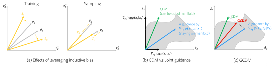
Figure 3: Conceptual illustration of Composable DMs and our proposed sampling method. (a) shows the effects of leveraging the inductive bias during training and sampling. Leveraging the inductive bias during the training may more disentangle the feature representation. On the other hand, the inductive bias can be used for balancing the amount of the content and the style during the sampling. (b) compares CDM and the joint guidance. The result based on CDM can be outside of manifold while the joint guidance stays on manifold. (c) shows the proposed GCDM. GCDM trades off between the independent guidance provided by CDM (stronger effects of the condition) and the joint guidance (more realistic). Corresponding experiment results can be found in Fig. 5, 6 (main paper) and Fig. 25 (supplementary).

Our framework is based on the LDM [42] architecture as it is faster to train and sample from, compared to pixel–based diffusion models. Let $x$ be an input image and $E_{LDM}$ and $D_{LDM}$ be the pretrained and fixed encoder and decoder respectively. The actual input space for our diffusion model is the low-dimensional latent space $z=E_{LDM}(x)$. The output of the reverse diffusion process is the low dimensional latent $\hat{z}_{0}$ which is then passed through the pretrained decoder as $x=D_{LDM}(\hat{z}_{0})$ to get the final image $\hat{x}_{0}$.

3.1 Learning Content and Style Latent spaces

Inspired by DiffAE [40] and similar approaches in GANs [29], we introduce a content encoder $E_{c}(\,\cdot\,;\psi)$ and a style encoder $E_{s}(\,\cdot\,;\phi)$ in our framework as shown in Fig. 2. The objective for training is formulated as:

$$\min_{\theta,\psi,\phi}\mathop{\mathbb{E}_{z_{0},\epsilon_{t}}}\left[\lVert\epsilon_{t}-\epsilon(z_{t},t,E_{c}(z_{0};\psi),E_{s}(z_{0};\phi);\theta)\rVert_{2}^{2}\right],$$

where $z_{t}$ is from the forward process, i.e., $z_{t}=q(z_{t}|z_{0})$. To ensure that the encoders capture different semantic factors of an image, we design the shape of $z_{s}$ and $z_{c}$ asymmetrically as done in  [39, 48, 21, 32, 29, 4]. The content encoder $E_{c}(z_{0};\psi)$ outputs a spatial layout mask $z_{c}\in\mathbb{R}^{1\times\frac{h}{4}\times\frac{w}{4}}$ where $w$ and $h$ are the width and height of $z_{0}$ latent. In contrast, $E_{s}(z_{0};\phi)$ outputs $z_{s}\in\mathbb{R}^{512\times 1\times 1}$ after global average pool layer to capture global high-level semantics. At each layer of the denoising UNet $\epsilon(\,\cdot\,;\theta)$, the style code $z_{s}$ is applied using channel-wise affine transformation along with timestep information ($t_{1}$, $t_{2}$, and $t_{3}$) while the content code $z_{c}$ is applied in a spatial manner as shown below.

$$\underbrace{t_{1}(1+\varphi^{\ell}(z_{c}))}_{\text{spatial-wise}}\odot\underbrace{(1+\zeta^{\ell}(z_{s}))\cdot(t_{2}(h^{\ell}+t_{3}))}_{\text{channel-wise}},$$ (1)

where $\varphi^{\ell}$ is a down or upsampling operation at $\ell$-th layer to make the dimensions of $\varphi^{\ell}(z_{c})$ and $h^{\ell}$ match, and $\zeta^{\ell}$ is a MLP layer to optimize $z_{s}$ particularly for $\ell$-th layer. $h^{\ell}$ denotes the group-normalized feature map at $\ell$-th layer from the denoising networks $\epsilon(\,\cdot\,;\theta)$, and $t_{1}$, $t_{2}$ and $t_{3}$ are timestep information from $\text{MLP}(\text{enc}(t))$ following sinusoidal embedding layer. Group Normalization is used, following the prior work [40].

3.2 Timestep Scheduling for Conditioning

It has been observed in [5, 6, 1] that low-frequency information, i.e., coarse features such as pose and facial shape are learned in the earlier timesteps (e.g., $0<\text{SNR(t)}<10^{-2}$) while high-frequency information such as fine–grained features and imperceptible details are encoded in later timesteps (e.g., $10^{0}<\text{SNR(t)}<10^{4}$) in the reverse diffusion process. Here, SNR(t) stands for signal-to-noise ratio per timestep [26].

Inspired by this, we introduce a weight scheduler for $z_{c}$ and $z_{s}$ that determines how much the content and the style conditions are applied into the denoising networks. We use the following schedule:

$$w_{c}(t) =\frac{1}{1+\exp{(-a(t-b))}}$$ (2)

$$w_{s}(t) =\frac{1}{1+\exp{(-a(-t+b))}},$$ (3)

where $a$ is a coefficient for determining how many timesteps content and style are jointly provided while $b$ indicates the timestep at which $w_{s}(t)\geq w_{c}(t)$. We also tried simple linear weighting schedule (decreasing for content and increasing for style with every timestep during the reverse diffusion process) and constant schedule but observed that the proposed schedule gave consistently better results (examples are provided in Section F.2 in the supplementary). We additionally evaluate using timestep scheduling during training. It is a promising future direction showing better decomposition between factors controlled by content and style (Section F.1 in the supplementary).

3.3 Generalized Composable Diffusion Models

As mentioned in Section 1, generalizing CDM by introducing the joint component can potentially improve composition of multiple conditions and enhancing controllability over the generation. Fig. 3 shows a conceptual illustration of the possible benefit of GCDM over CDM. Let $z_{s}^{*}$ and $z_{c}^{*}$ be the ground-truth content and style features that are not observed in Fig. 3 (a). The approximated content and the style features $\hat{z}_{c}$ and $\hat{z}_{s}$ can be better separated by leveraging the inductive bias during training. Using the inductive bias only during sampling, would represent scaling due to the variation in their magnitude across timesteps. Note that the approximated $\hat{z}_{c}$ and $\hat{z}_{s}$ are used as the axes in (b) and (c). Fig. 3 (b) shows an example that the content and the style guidances from CDM generate unrealistic samples because the combined guidance is outside the manifold. On the contrary, the joint guidance helps keep the generation within the manifold. (c) visualizes the proposed GCDM which can be seen as a linear interpolation between CDM and the joint guidance. GCDM has the added advantage of enabling separate controls for style, content and realism. Moreover, CDM and the joint guidance are special cases of GCDM. Hence, we argue that it is helpful to derive a generalized composing method without constraining the style and content to be conditionally independent as done in [34]. We would like to sample images given multiple conditions (i.e., style and content in our case), which we formulate as sampling from $\tilde{p}(x_{t}|c_{1},c_{2})\propto p(x_{t})[p(c_{1},c_{2}|x_{t})^{\lambda}(p(c_{1}|x_{t})^{\beta_{1}}p(c_{2}|x_{t})^{\beta_{2}})^{1-\lambda}]^{\alpha}$, where $\alpha\geq 0$ controls the overall strength of conditioning, $\lambda\in[0,1]$ controls the trade-off between the dependent and independent conditional information, and $\beta_{1}$ and $\beta_{2}$ control the weight for style and content information. The guidance gradient in terms of the denoising network $\epsilon$ (which may depend on zero, one or both conditions) is as follows:

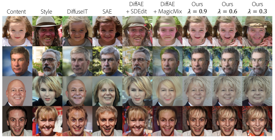
Figure 4: Comparison of the proposed model with baselines for reference based image translation on FFHQ dataset. Our method generates more plausible, realistic combinations of the content and style images with better controllability. Other models either show poorer performance or lack sufficient controllability.

$$\nabla_{x_{t}}\log\tilde{p}(x_{t}|c_{1},c_{2})=$$ (4)

$$\underbrace{\epsilon(x_{t},t)}_{\nabla\log p(x_{t})}+\alpha[\lambda\underbrace{(\epsilon(x_{t},t,c_{1},c_{2})-\epsilon(x_{t},t))}_{\nabla\log p(c_{1},c_{2}|x_{t})}$$ (5)

$$+(1-\lambda)\underbrace{{\color[rgb]{0,0,0}\sum_{i=\{1,2\}}}\beta_{i}\underbrace{(\epsilon(x_{t},t,c_{i})-\epsilon(x_{t},t))}_{\nabla\log p(c_{i}|x_{t})}}_{\nabla\log p(c_{1}|x_{t})p(c_{2}|x_{t})}]\,,$$ (6)

If $\lambda=0$, this simplifies to CDM [34] and thus can be seen as a generalization of it. In the following experiments on image translation, $\beta_{1}$ and $\beta_{2}$ denote $\beta_{s}$ and $\beta_{c}$, respectively. The detailed derivation and the effect of various hyperparameters are in Sections B and D.1 in the supplementary.

Note that GCDM and timestep scheduling are generic sampling techniques for diffusion models that can also be applied to other tasks beyond image translation (Fig. 5).

4 Experiments

Table 1: Quantitative comparison between the proposed and baseline models using FID and LPIPS on FFHQ dataset.

DiffuseIT [30] SAE [39] DiffAE+SDEdit [40, 37] DiffAE+MagicMix [33] Ours($\lambda=0.9$) Ours($\lambda=0.6$) Ours($\lambda=0.3$) FID 29.99 25.06 26.63 84.55 11.99 13.40 15.45 LPIPS 0.47 0.39 0.64 0.41 0.34 0.42 0.49

We comprehensively evaluate the proposed model on image to image translation and additionally show qualitative examples of GCDM and CDM on text to image composition with stable diffusion. Implementation details are provided in Section D. For sampling, we use reverse DDIM [40] approach conditioned on the content image and its corresponding content and style codes to get $x_{T}$ instead of sampling random noise unless otherwise mentioned. This helps with better identity preservation for faces. Analysis on the effects of reverse DDIM is provided in Section D.2.

4.1 Experimental Setup

Datasets
We train different models on the commonly used datasets such as AFHQ [7], FFHQ [22] and LSUN-church [52].

Baselines
DiffuseIT: The most similar work to ours based on diffusion models is DiffuseIT [30] that tackles the same problem formulation. We compare our results with DiffuseIT using their pretrained model and default parameters.
DiffAE+SDEdit: Since Diffusion Autoencoder [40] does not directly support image-to-image translation, we combine that with SDEdit [37]. The input image for the reverse process is $x_{600}$ (chosen empirically) obtained as $q(x_{600}|x_{c})$ by running the forward process on the content image. The semantic feature $z_{sem}$ from the semantic encoder of DiffAE is used given the style image $x_{s}$.
DiffAE+MagicMix: We also combine MagixMix [33] with DiffAE. Similar to DiffAE+SDEdit, this model takes $x_{600}$ from $x_{c}$ as input and $z_{sem}$ from $x_{s}$ as conditioning. Additionally, at each timestep, the approximated previous timestep $\hat{x}_{t-1}$ is combined with $x_{t-1}$ from the content image $x_{c}$, i.e., $\hat{x}_{t-1}=v\hat{x}_{t-1}+(1-v)q(x_{t-1}|x_{c})$. For this experiment, $v=0.5$ is used and the noise mixing technique is applied between $t=[600,300]$.
SAE: Swapping Autoencoder [39] based on GAN [14] is also evaluated. Since the available pretrained model is on the resolution of 512, we resize the generated results to 256 for fair comparison.

Evaluation Metrics
FID: We use the commonly used Fréchet inception distance (FID) [17] to ensure the generated samples are realistic. We follow the protocol proposed in [7] for reference based image translation. To obtain statistics from generated images, 2000 test samples are used as the content images and five randomly chosen images from the rest of the test set are used as style images for each content image to generate 10000 synthetic images.
LPIPS: Even though FID evaluates realism of the generations, the model could use just content and ignore style (or vice versa) and still get good FID. Following [7], we use LPIPS score obtained by measuring the feature distances between pairs of synthetic images generated from the same content image but with different style images. Higher LPIPS indicates more diverse results. It is ideal for the model to tradeoff between LPIPS and FID, i.e incorporate enough style information from different style images for the same content image (increasing LPIPS) but without going out of the real distribution (decreasing FID).

4.2 Comparison with Existing Works

In this section, we compare the reference-based image translation performance of the proposed model with baseline models on FFHQ dataset.
Qualitative Results.
Fig. 4 visually shows example generations from different techniques. We observe that DiffAE+SDEdit loses content information while DiffAE+MagicMix generates unnatural images that naively combine the two images. This indicates that a single latent space even with additional techniques such as SDEdit and MagicMix is not suitable for reference based image translation. DiffuseIT and SAE models maintain more content information but does not transfer enough information from the style image and have no control over the amount of information transferred from style.

An important benefit of the proposed method is better controllability. By manipulating $\lambda$, we can control how much guidance is applied. In Fig. 4, decreasing $\lambda$ increases the effect of style from the style image when $\beta_{c}=0$ and $\beta_{s}=1$, where $\beta_{c}$ and $\beta_{s}$ are the weights for each conditional guidance (Eq. 4–6). For example, the man on the second row has more wrinkles and beard as $\lambda$ decreases. Visualizations on the behavior of each hyperparameter are provided in Fig. 10 in the supplementary.
Quantitative Results.
Table 1 shows quantitative comparison in terms of FID and LPIPS metrics on FFHQ dataset. Our variants generate images that are realistic as indicated by the lowest FID scores compared with other models while also performing better on diversity as measured by the highest LPIPS except for DiffAE+SDEdit method. However, DiffAE+SDEdit does not show meaningful translation of style onto the content image. DiffAE+MagicMix shows the worst performance because of its unrealistic generation. SAE and DiffuseIT show lower LPIPS score than ours, indicating that it translates very little information from the style image onto the content image. We can also observe that increasing $\lambda$ (when $\beta_{c}=0$ and $\beta_{s}=1$) makes LPIPS worse while improving FID. In other words, the stronger the joint guidance is, the more realistic but less diverse the generations. This verifies our assumption in Fig. 3 that the joint component has an effect of pushing the generations into the real manifold.

4.3 Effect of GCDM and Timestep Scheduling

CDM vs GCDM.
The key benefit of leveraging GCDM is that the guidance by GCDM would help keep the sample on the real manifold and thereby generate more realistic images.

Table 2: FID comparisons between SAE and our model with CDM and GCDM on AFHQ dataset.

SAE CDM GCDM GCDM ($\lambda=0.9$) ($\lambda=1.0$) FID 9.29 10.57 9.75 8.58 LPIPS 0.45 0.59 0.59 0.57

We compare SAE [39] (the best performing baseline) and ours on AFHQ dataset in Table 2. The joint guidance ($\lambda=1$) gets the lowest FID indicating that the generations are more realistic as it pulls the guided results to be within the real data manifold. We can also see that GCDM can be thought of as interpolating between CDM and the joint guidance term, since FID for GCDM ($\lambda=0.9$) is in between the joint and CDM. By comparing LPIPS and FID of the variants of GCDM, we can see that the outputs become less diverse as realism is increased. SAE shows worse performance than ours in terms of both diversity and realism. The qualitative comparisons can be found in Fig. 25 in the supplementary.
Generalizability of GCDM.
We also compare the performance of CDM and GCDM in composing text prompts for text to image generation using Stable Diffusion V2[42] in Fig. 5. The phrases before and after ‘and’ are used as the first and the second guidance terms in Eq. 6. The full sentence is used to represent the joint conditioning.

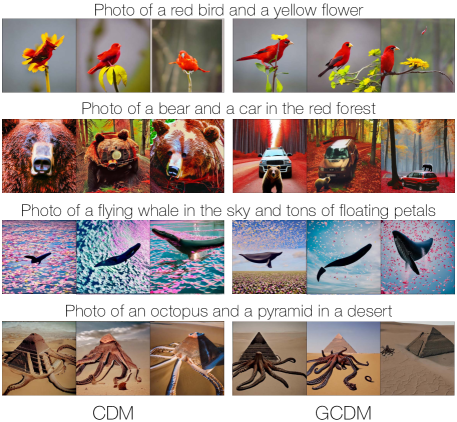
Figure 5: GCDM vs CDM for text-to-image generation with Stable Diffusion. We can observe that CDM generates unnatural images (e.g., blending two objects) that may be out of the real manifold while GCDM ensures realistic generations (e.g., combining two objects in a realistic way).

As shown in Fig. 5, CDM tends to fail in composing multiple conditions if both conditions contain object information. For example, the red bird and the yellow flower are merged in two out of three generations using CDM. On the other hand, GCDM consistently shows better compositions in the generated images. This emphasizes that GCDM is a generalized formulation for composing multiple conditioning inputs providing more control to the user in terms of realism and diversity as illustrated in Fig. 3. Additional results and the used GCDM hyperparameters can be found in Fig. 28.
Effect of Timestep Scheduling.
To more carefully analyze the effect of time-step scheduling when combined with GCDM or CDM, we alter the time-step scheduling so that there is at least a 0.1 weight on style or content. Specifically, we change the upper and lower bounds of the the sigmoid to be 0.1 and 0.9 in Eq 2 and 3, e.g., $w_{c}^{\prime}(t)=0.8w_{c}(t)+0.1$. The results can be seen in Table 3 and Fig. 6. Without timestep scheduling, GCDM shows better performance in both FID (realism) and LPIPS (diversity). Combined with timestep scheduling, both CDM and GCDM show meaningful improvements in FID in exchange for losing diversity. This is because, timestep scheduling improves content identity preservation, e.g., pose and facial structure causing less variations in structural information and consequently lower LPIPS/diversity. Additionally, timestep scheduling with GCDM variants show better FID or LPIPS than CDM depending on the strength of guidance terms showing varied control over the generations.

Table 3: FID comparisons between CDM and GCDM with and without the timestep scheduling in FFHQ dataset. Best method without timestep scheduling is highlighted in bold and with timestep scheduling is highlighted with a *.

w/o schedule w/ schedule CDM GCDM CDM GCDM ($\beta_{c}=1$) GCDM ($\beta_{s}=1$) FID 21.43 14.46 10.50 10.21* 10.61 LPIPS 0.47 0.51 0.31 0.28 0.33*

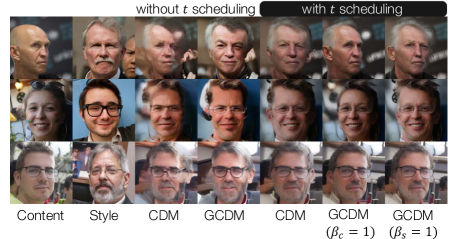
Figure 6: Effect of timestep scheduling in CDM and GCDM. Timestep scheduling improved the results of both CDM and GCDM and gives the best results when combined with GCDM.

Figure 7: Visualization of the effect of each guidance term (described in Eq. 4-6) on generation. $x_{T}$ is randomly sampled.

4.4 Analysis and Discussion

In this section, we analyze the importance of each of the components of our framework using AFHQ and LSUN-church dataset and aim to better understand the content and style latent spaces. Further analysis and results based PCA, latent interpolation and K-Nearest Neighbor are provided in Section E.1, E.2 and E.3 respectively in the supplementary.
Visualization of Each Guidance Term.

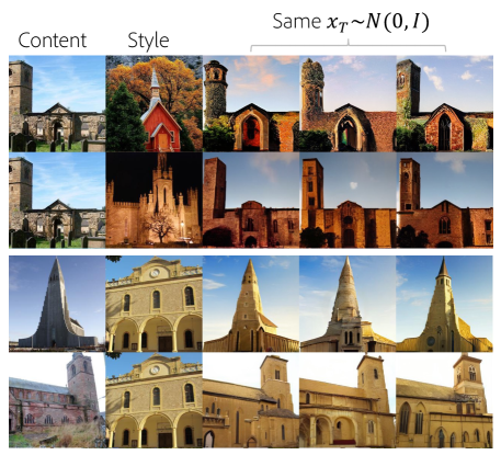
Figure 8: Example generations on LSUN-church dataset showing that the content and style codes are robust to changes. $x_{T}$ is randomly sampled.

The proposed GCDM in Section 3.3 has guidance from three terms, the joint distribution of style and content and style and content codes separately. Fig. 7 shows comparison of the effect of these terms. Columns 3 shows images generated only using guidance from content image. It can be seen that the generated animals are not the same as the content image but has the exact same structure and pose. Similarly, columns 4 shows generations when only style guidance is used. Since content information is not used at all, the pose is random while the style such as color, fur etc. corresponds to the style image. Column 5 shows result of joint guidance whereas the last column shows generations using GCDM. It can be observed that GCDM with $\beta_{s}=1.0$ has more semantic information from the style than the joint guidance.
Classifier-based comparisons.
To further understand what kind of attributes are encoded in style and content latent spaces, we use pretrained classifiers to predict the attributes of translated images and compare with the original style and content images. We sample 2000 random images from test set to use as $x_{c}$ and another 2000 as $x_{s}$ to form 2000 content-style pairs. Next, we acquire the translated output $x_{o}$ and corresponding pseudo labels $y_{c}$, $y_{s}$ and $y_{o}$ by leveraging an off-the-shelf pretrained attribute classifier (EasyFace). In Table 4, we show the probabilities that the final generated image $x_{o}$ has an attribute from content image as $p(y_{c}^{att}=y_{o}^{att})$ and likewise for style image.

Both ours and SAE are designed to make $z_{s}$ encode global high-level semantics, e.g., Gender, Age, etc. Thus, methods would show ideal performance if $y_{o}^{att}=y_{s}^{att}\neq y_{c}^{att}$. We see that most global attributes come from the content image for SAE indicating conservative translations from the style image (as seen in Fig. 4 and lower LPIPS in Table 1). In contrast, ours has a controllable way of deciding the strength of attributes from the style image through $\lambda$. The lower the value of $\lambda$, the more disentangled and consistent the attributes will be in the generations.

Table 4: Classifier-based comparisons in FFHQ.

Probability Att. is Equal (%) $x_{c}$ $x_{s}$ Gender Age Race Gender Age Race SAE 65.95 62.36 50.40 34.05 26.40 27.91 Ours ($\lambda=0.9$) 65.14 53.79 53.31 34.86 31.60 28.51 Ours ($\lambda=0.25$) 26.61 25.94 31.73 73.39 56.77 44.48

Information Encoded in Each Latent Space.
We analyze the role of the denoising network $\epsilon_{\theta}$ and the encoders $E_{c}$ and $E_{s}$ by analyzing what information is encoded in the respective latent spaces. Fig. 8 and Fig. 9 show the role of $\epsilon_{\theta}$ in the reverse process evaluated on LSUN-church dataset. Fig. 8 shows the results of fixing the content while varying the style images (and vice versa). $x_{T}$ is fixed as well to reduce the stochasticity. The remaining stochasticity comes from the white noise at each timestep during the reverse process. From the results, we can see that the structure information is maintained while style information changes according to the style image (and vice versa) as we intended.

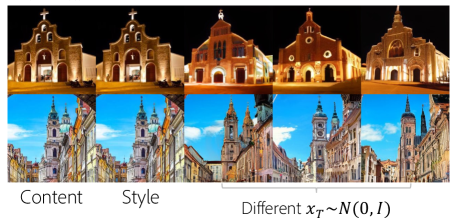
Figure 9: Example showing the role of the denoising network during sampling when content and style codes are unchanged. $x_{T}$ is randomly sampled.

Similarly, in Fig. 9 we forward the same image to content and style encoders while the generation starts from different random noise $x_{T}$. The images show that the denoising network play a role in stochasticity since the outputs have consistent shape, color and texture information while minor details of the buildings or clouds are changed.

5 Conclusion

We propose a novel framework for enhancing controllability in image conditioned diffusion models for reference based image translation and image manipulation. Our content and style encoders trained along with the diffusion model do not require additional objectives or labels to learn to decompose style and content from images. The proposed generalized composable diffusion model extends CDM for a more generalized scenario. It shows significantly better performance when compared with CDM for translation as well as compositing text prompts. We also build on the inductive bias and show that timestep dependent weight schedules for conditioning inputs can help improve overall results and controllability. Additionally, the learned latent spaces are observed to have desirable properties like PCA based attribute manipulation and smooth interpolations. Quantitative and qualitative evaluation shows the benefits of the proposed sampling techniques.

Appendix A Overview

Through this paper, we propose novel ways to condition and control diffusion models for image manipulation and translation. Our contributions can be summarized as follows:

• Content and Style Latent Space:
  We learn separate content and style latent spaces that correspond to different semantic factors of an image. This lets us control these factors separately to perform reference based image translation as well as controllable generation and image manipulation.

• Timestep Scheduling:
  We leverage the inductive bias of diffusion models and propose timestep dependent weight schedules to compose information from content and style latent codes for better translation.

• Generalized Composable Diffusion Model (GCDM):
  We extend Composable Diffusion Models (CDM) to allow for dependency between conditioning inputs, in our case, content and style. This results in significantly better generations and more controllability.

We believe that the proposed sampling techniques are applicable for controllable generation in general and not specific to image translation. To support our claims and show the ability of the proposed techniques for various problem formulations, we show additional results with various settings and parameters in appendix. We also provide more details on the experimental setup, models and parameters used to get the results shown in the main paper. Below is a list of contents in appendix.

1. We start by deriving the proposed Generalized Composable Diffusion Model in Section B when the conditioning inputs are not constrained to be independent.

2. We explain the training details, and show better identity preservation on faces and other datasets by combining the proposed sampling techniques with deterministic reverse DDIM [40] sampling in Section D.

3. We show that the learned style and content space can be used for attribute specific image manipulation in Section E. We also show that style and content interpolations between images can be used for for style/content transfer and mixing. We also analyze what the content and style encoders have learned by visualizing the nearest neighbors in content and style space respectively in Section E.3

4. The proposed timestep scheduling was only used during inference in the main paper. In Section F.1, we evaluate a model trained with timestep scheduling to implicitly learn a mixture–of–experts [1] model by virtue of varying the conditional information at each timestep instead. We show these results on FFHQ in Fig. 22. We also show experiments with different timestep schedule functions in Section F.2

5. We finally provide some additional results such as text2image synthesis and reference based image translation in Section G.

Appendix B Derivation for the proposed Generalized Composable Diffusion Model

One of the interesting properties of DM is that a score function of the class conditional density $p(x|y)$ can be obtained by multiplying a score function of the marginal density $p(x)$ (i.e., an unconditionally trained DM) and a gradient of the likelihood $p(y|x)$ (i.e., a classifier). This was utilized in [9] for classifier guidance. Since classifier guidance requires a pretrained classifier and lacks the ability to provide specific guidance, [19] proposed classifier–free guidance to control the generation.

B.1 Classifier-free Guidance [19]

$$\nabla_{x_{t}}\log p(x_{t}|c) =\nabla_{x_{t}}\log p(x_{t},c)$$ (7)

$$\nabla_{x_{t}}\log p(x_{t},c) =\nabla_{x_{t}}\log p(x_{t})p(c|x_{t})$$ (8)

$$=\nabla_{x_{t}}\log p(x_{t})\frac{p(x_{t}|c)}{p(x_{t})}$$ (9)

$$=\nabla_{x_{t}}\log p(x_{t})+\left(\nabla_{x_{t}}\log p(x_{t}|c)-\nabla_{x_{t}}\log p(x_{t})\right)$$ (10)

$$=\epsilon(x_{t},t)+\left(\epsilon(x_{t},t,c)-\epsilon(x_{t},t)\right).$$ (11)

Practically, $\epsilon(x_{t},t)+\alpha\left(\epsilon(x_{t},t,c)-\epsilon(x_{t},t)\right)$ is used where $\alpha$ is a temperature controlling the condition effect.

The $\nabla_{x_{t}}\log p(x_{t}|c)-\nabla_{x_{t}}\log p(x_{t})$ can be seen as an implicit classifier.

B.2 Composable Diffusion Models [34]

$$\nabla_{x_{t}}\log p(x_{t}|c_{1},c_{2}) =\nabla_{x_{t}}\log p(x_{t},c_{1},c_{2})$$ (12)

$$\nabla_{x_{t}}\log p(x_{t},c_{1},c_{2}) =\nabla_{x_{t}}\log p(x_{t})p(c_{1},c_{2}|x_{t})\quad assuming\,\,\,C_{1}\perp C_{2}|X_{t}$$ (13)

$$=\nabla_{x_{t}}\log p(x_{t})p(c_{1}|x_{t})p(c_{2}|x_{t})$$ (14)

$$=\nabla_{x_{t}}\log p(x_{t})\frac{p(x_{t}|c_{1})}{p(x_{t})}\frac{p(x_{t}|c_{2})}{p(x_{t})}$$ (15)

$$=\nabla_{x_{t}}\log p(x_{t})+\sum_{i}\left(\nabla_{x_{t}}\log p(x_{t}|c_{i})-\nabla_{x_{t}}\log p(x_{t})\right)$$ (16)

$$=\epsilon(x_{t},t)+\sum_{i}\left(\epsilon(x_{t},t,c_{i})-\epsilon(x_{t},t)\right)$$ (17)

Similar to the Classifier-free Guidance, $\alpha$ is used as well.

B.3 Generalized Composable Diffusion Models

$$\nabla_{x_{t}}\log p(x_{t}|c_{1},c_{2}) =\nabla_{x_{t}}\log p(x_{t},c_{1},c_{2})$$ (18)

$$\nabla_{x_{t}}\log p(x_{t},c_{1},c_{2}) =\nabla_{x_{t}}\log p(x_{t})p(c_{1},c_{2}|x_{t})\quad NOT\,\,assuming\,\,\,C_{1}\perp C_{2}|X_{t}$$ (19)

$$=\nabla_{x_{t}}\log p(x_{t})p(c_{1}|c_{2},x_{t})p(c_{2}|x_{t})$$ (20)

$$=\nabla_{x_{t}}\log p(x_{t})p(c_{2}|x_{t})\left(\frac{p(c_{2}|c_{1},x_{t})p(c_{1}|x_{t})}{p(c_{2}|x_{t})}\right)$$ (21)

$$=\nabla_{x_{t}}\log p(x_{t})p(c_{2}|x_{t})p(c_{1}|x_{t})\left(\frac{p(c_{2}|c_{1},x_{t})}{p(c_{2}|x_{t})}\right)$$ (22)

$$=\nabla_{x_{t}}\log p(x_{t})p(c_{2}|x_{t})p(c_{1}|x_{t})\left(\frac{p(c_{1},c_{2}|x_{t})}{p(c_{1}|x_{t})p(c_{2}|x_{t})}\right)$$ (23)

$$=\nabla_{x_{t}}\log\frac{p(x_{t}|c_{2})p(x_{t}|c_{1})}{p(x_{t})}\left(\frac{\frac{p(x_{t}|c_{1},c_{2})}{p(x_{t})}}{\frac{p(x_{t}|c_{1})p(x_{t}|c_{2})}{p(x_{t})^{2}}}\right)$$ (24)

$$=\nabla_{x_{t}}\log\frac{p(x_{t}|c_{2})p(x_{t}|c_{1})}{p(x_{t})}\left(\frac{p(x_{t}|c_{1},c_{2})p(x_{t})}{p(x_{t}|c_{1})p(x_{t}|c_{2})}\right)$$ (26)

$$=\underbrace{-\epsilon(x_{t},t)+\epsilon(x_{t},t,c_{2})+\epsilon(x_{t},t,c_{1})}_{\raisebox{-0.9pt}{1}⃝}$$ (27)

$$\quad+\underbrace{\left\{\epsilon(x_{t},t,c_{1},c_{2})+\epsilon(x_{t},t)-\left(\epsilon(x_{t},t,c_{1})+\epsilon(x_{t},t,c_{2})\right)\right\}}_{\raisebox{-0.9pt}{2}⃝}$$ (28)

The term $\raisebox{-0.9pt}{1}⃝$ can be seen as a guidance from implicit classifiers.

$$\left\{\epsilon(x_{t},t,c_{1},c_{2})+\epsilon(x_{t},t)-\left(\epsilon(x_{t},t,c_{1})+\epsilon(x_{t},t,c_{2})\right)\right\}$$ (29)

$$=\left\{\epsilon(x_{t},t,c_{1},c_{2})-\epsilon(x_{t},t)-\left(\epsilon(x_{t},t,c_{1})-\epsilon(x_{t},t)\right)-\left(\epsilon(x_{t},t,c_{2})-\epsilon(x_{t},t)\right)\right\}$$ (30)

$$=\{\nabla_{x_{t}}\log p(x_{t}|c_{1},c_{2})-\nabla_{x_{t}}\log p(x_{t})$$ (31)

$$\quad-\left(\nabla_{x_{t}}\log p(x_{t}|c_{1})-\nabla_{x_{t}}\log p(x_{t})\right)-\left(\nabla_{x_{t}}\log p(x_{t}|c_{2})-\nabla_{x_{t}}\log p(x_{t})\right)\}$$ (32)

$$=\left\{\nabla_{x_{t}}\log p(c_{1},c_{2}|x_{t})-\left(\nabla_{x_{t}}\log p(c_{1}|x_{t})+\nabla_{x_{t}}\log p(c_{2}|x_{t})\right)\right\}$$ (33)

Similarly, the term $\raisebox{-0.9pt}{2}⃝$ can be rearranged as

$$-\epsilon(x_{t},t)+\epsilon(x_{t},t,c_{2})+\epsilon(x_{t},t,c_{1})$$ (34)

$$=\epsilon(x_{t},t)+\left(\epsilon(x_{t},t,c_{2})-\epsilon(x_{t},t)\right)+\left(\epsilon(x_{t},t,c_{1})-\epsilon(x_{t},t)\right)$$ (35)

$$=\nabla_{x_{t}}\log p(x_{t})+\nabla_{x_{t}}\log p(c_{2}|x_{t})+\nabla_{x_{t}}\log p(c_{1}|x_{t})$$ (36)

By rearranging those two terms and adding hyperparameters $\alpha$, $\lambda$ and $\{\beta_{c},\beta_{s}\}$, the proposed GCDM method can be obtained.

$$\nabla_{x_{t}}\log\tilde{p}(x_{t}|c_{1},c_{2})=\underbrace{\epsilon(x_{t},t)}_{\nabla\log p(x_{t})}+\alpha\left[\lambda\underbrace{(\epsilon(x_{t},t,c_{1},c_{2})-\epsilon(x_{t},t))}_{\nabla\log p(c_{1},c_{2}|x_{t})}+(1-\lambda)\underbrace{\sum_{i=1}^{2}2\beta_{i}\underbrace{(\epsilon(x_{t},t,c_{i})-\epsilon(x_{t},t))}_{\nabla\log p(c_{i}|x_{t})}}_{\nabla\log p(c_{1}|x_{t})p(c_{2}|x_{t})}\right]\,,$$ (37)

where $\alpha\geq 0$ and $0\leq\lambda\leq 1$. $\alpha$ controls the strength of conditioning while $\lambda$ controls whether a dependency between conditions is allowed or whether the conditions are assumed to be independent. $\{\beta_{c},\beta_{s}\}$ controls the strength of each condition, and $\beta_{c}+\beta_{s}=1$. In theory, assuming $\beta_{c}=\beta_{s}=1$, this will sample from a model defined as:

$$\tilde{p}(x_{t}|c_{1},c_{2})\propto p(x_{t})[p(c_{1},c_{2}|x_{t})^{\lambda}(p(c_{1}|x_{t})p(c_{2}|x_{t}))^{1-\lambda}]^{\alpha}\,,$$ (38)

so it is a geometric average between the joint classifier $p(c_{1},c_{2}|x_{t})$ and the product of two independent classifiers $p(c_{1}|x_{t})p(c_{2}|x_{t})$. If $\lambda=0$, then this simplifies to the composable model, thus this can be seen as a generalization of this method. Furthermore, if $\lambda=1$ and $\alpha=1$, it is reduced to the simple joint conditional model $\epsilon(x_{t},t,c_{1},c_{2})$.

Appendix C Preliminaries on Diffusion Models

Diffusion Models [46, 18] are one class of generative models that map the complex real distribution to the simple known distribution. In high level, DMs aim to train the networks that learn to denoise a given noised image and a timestep $t$. The noised image is obtained by a fixed noising schedule. Diffusion Models [46, 18] are formulated as $p_{\theta}(x_{0})$. The marginal $p_{\theta}(x_{0})$ can be formulated as a marginalization of the joint $p_{\theta}(x_{0:T})$ over the variables $x_{1:T}$, where $x_{1},...x_{T}$ are latent variables, and $p(x_{T})$ is defined as standard gaussian. Variational bound of negative log likelihood of $p_{\theta}(x_{0})$ can be computed by introducing the posterior distribution $q(x_{1:T}|x_{0})$ with the joint $p_{\theta}(x_{0:T})$. In Diffusion Models [46, 18], the forward process $q(x_{1:T}|x_{0})$ is a predefined Markov Chain involving gradual addition of noise sampled from standard Gaussian to an image. Hence, the forward process can be thought of as a fixed noise scheduler with the $t$-th factorized component $q(x_{t}|x_{t-1})$ represented as: $q(x_{t}|x_{t-1})=\mathcal{N}(x_{t};\sqrt{1-\beta_{t}}x_{t-1},\beta_{t}I)$, where $\beta_{t}$ is defined manually. On the other hand, the reverse or the generative process $p_{\theta}(x_{0:T})$ is modelled as a denoising neural network trained to remove noise gradually at each step. The $t$-th factorized component $p_{\theta}(x_{t-1}|x_{t})$ of the reverse process is then defined as, $\mathcal{N}(x_{t-1}|\mu_{\theta}(x_{t},t),\Sigma(x_{t},t))$. Assuming that variance is fixed, the objective of Diffusion Models (estimating $\mu$ and $\epsilon$) can be derived using the variational bound [46, 18] (Refer the original papers for further details).

Following Denoising Diffusion Probabilistic Models [18] (DDPM), Denoising Diffusion Implicit Model [47] (DDIM) was proposed that significantly reduced the sampling time by deriving a non-Markovian diffusion process that generalizes DDPM. The latent space of DDPM and DDIM has the same capacity as the original image making it computationally expensive and memory intensive. Latent Diffusion Models [42] (LDM) used a pretrained autoencoder [12] to reduce the dimension of images to a lower capacity space and trained a diffusion model on the latent space of the autoencoder, reducing time and memory complexity significantly without loss in quality.

All our experiments are based on LDM as the base diffusion model with DDIM for sampling. However the techniques are equivalently applicable to any diffusion model and sampling strategy.

Appendix D Implementation Details

We build our models on top of LDM codebase. For FFHQ and LSUN-church, we train our model for two days with eight V–100 GPUs. The model for AFHQ dataset is trained for one and a half days with the same device. All models are trained for approximately 200000 iterations with a batch size of 32, 4 samples per GPU without gradient accumulation. All models are trained with 256$\times$256 images with a latent $z$ size of 3$\times$64$\times$64. The dimensions of content code $z_{c}$ is 1$\times$8$\times$8 while that of style code $z_{s}$ is 512$\times$1$\times$1. $t_{1},t_{2}$ and $t_{3}$ from Eq. 1 in the main paper are timestep embeddings learned to specialize according to the latent code they are applied for to support learning different behavior for content and style features at different timesteps. We also experimented with different sizes for content and style code and chose these for best empirical performance. The content encoder takes as input $z$ and outputs $z_{c}$ following a sequence of ResNet blocks. The style encoder has a similar sequence of ResNet blocks followed by a final global average pooling layer to squish the spatial dimensions similar to the semantic encoder in [40].

To support GCDM during sampling, we require the model to be able to generate meaningful scores and model the style, content and joint distributions. Hence, during training we provide only style code, only content code and both style and content code all with probability 0.3 (adding up to 0.9) and no conditioning with probability 0.1 following classifier–free guidance literature. This helps learn the conditional and unconditional models that are required to use the proposed GCDM formulation. The code will be released upon acceptance of the paper.

During sampling, without reverse DDIM, if all the joint, conditionals, and unconditional guidance are used, sampling time for a single image is 10 seconds. With reverse DDIM to get $x_{T}$ where T is the final timestep, it takes 22 seconds. This might be lesser if reverse DDIM is stopped early and generation happens from the stopped point. Specific hyperparameters used to generate results in the main paper and appendix are provided in Table. 5.

Table 5: Hyperparameters used to generate the figures in the main paper and appendix. Timestep scheduling is only used in the sampling process. The parenthesis in the second column indicates the number of steps we used for sampling. Note that $\beta_{c}=1-\beta_{s}$.

Main paper Dataset sampler $x_{T}$ $\alpha$ $\lambda$ $\beta_{s}$ $a$ $b$ scheduler FFHQ DDIM+SDEdit (60) reverse DDIM 1.5 0.9 1.0 0.025 550 sigmoid LSUN-church DDIM (100) $q(x_{991}|x_{0})$ 2.0 0.5 0.0 - - - AFHQ DDIM+SDEdit (60) $q(x_{591}|x_{0})$ 3.0 0.75 1.0 - - - Appendix FFHQ DDIM (100) reverse DDIM 1.5 0.9 1.0 0.025 550 sigmoid LSUN-church DDIM (100) reverse DDIM 5.0 0.5 0.0 0.025 600 sigmoid

D.1 Choice of Hyperparameters

We show results with various sets of parameters that can be used to control the effect of content, style and joint guidance in the generation in Fig. 10. The gray dotted box represents a baseline that we start from, and the rest of the other columns show the effects of each hyperparameter. As can be seen in the figure, each hyperparameter can be modified to get varying effects from style, content and joint guidance to get desirable results.

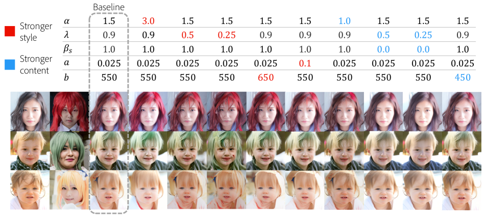
Figure 10: Example generations for different set of hyperparameters showing the effect of varying the controllable parameters during sampling. All generations start from $x_{T}$ obtained from reverse DDIM sampling using the content image.

We note that $\alpha$ works similar to classifier guidance scale in diffusion models like [42] and finding a good one when fixing $\lambda=1$, $a=0.025$, $b=500$ takes lesser time (as independent content and style guidance is not provided when $\lambda=1$). If the joint guidance has weaker style in the generations, it is recommended to modify $\lambda$ by setting $\beta_{s}=1$. We find that this setting mostly gives good results. In rare cases when the style changes are limited even with smaller $lambda$, increasing $b$ is another option. Modifying $a$ has relatively small effects on content and style specifically.

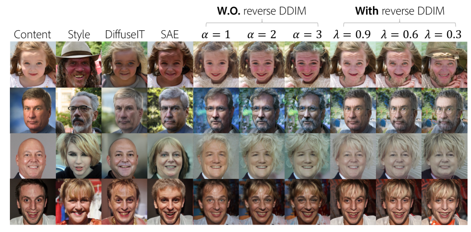
Figure 11: Comparisons between with and without reverse DDIM sampling for FFHQ model. We use the proposed GCDM and timestep scheduling during sampling. We can clearly see better identity preservation than not using reverse DDIM, on par with SAE [39] while still providing better controllability.

D.2 Identity Preservation

We notice that when the proposed sampling technique is used with randomly sampled noise $x_{T}$ for reference based image translation or manipulation, particularly on FFHQ dataset, that the identity of the content image is not preserved. This is an important aspect of image manipulation for faces. One of the ways to preserve better identity is to use the deteministic reverse DDIM process described in [40] to obtain $x_{T}$ that corresponds to a given content image. To do this, we pass the content image to both the content and style encoders as well as the diffusion model to get $x_{T}$ that reconstructs the content image. This $x_{T}$ is then used along with content code from content image and style code from style image to generate identity preserving translation.

The comparisons between with and without reverse DDIM during sampling are provided in Fig. 11. Columns 3-7 are the results reported in our main paper (Fig. 4), and Columns 8-10 are the results from using reverse DDIM. We can see that style is translated well on to the content image while preserving the identity of the content image. In contrast to SAE [39] that preserves better identity by trading of magnitude of style applied, our approach provides the ability to control the magnitude of identity preservation and style transfer independently.

Additional comparisons between with and without reverse DDIM are provided in Fig. 13 and 13. We can see that the results with reverse DDIM better preserves the content identity while applying the style reasonably. On the other hand, the results without reverse DDIM have stronger impact of style with lesser identity preservation, which may be preferable in non-face domains such as abstract or artistic images or for semantic mixing.

Table 6: Quantitative comparison between the variants of ours with and without reverse ddim.

w/o schedule w/ schedule Ours($\alpha=1.0$) Ours($\alpha=2.0$) Ours($\alpha=3.0$) Ours($\lambda=0.9$) Ours($\lambda=0.6$) Ours($\lambda=0.3$) FID 20.38 23.68 26.45 11.99 13.40 15.45 LPIPS 0.53 0.57 0.6 0.34 0.42 0.49

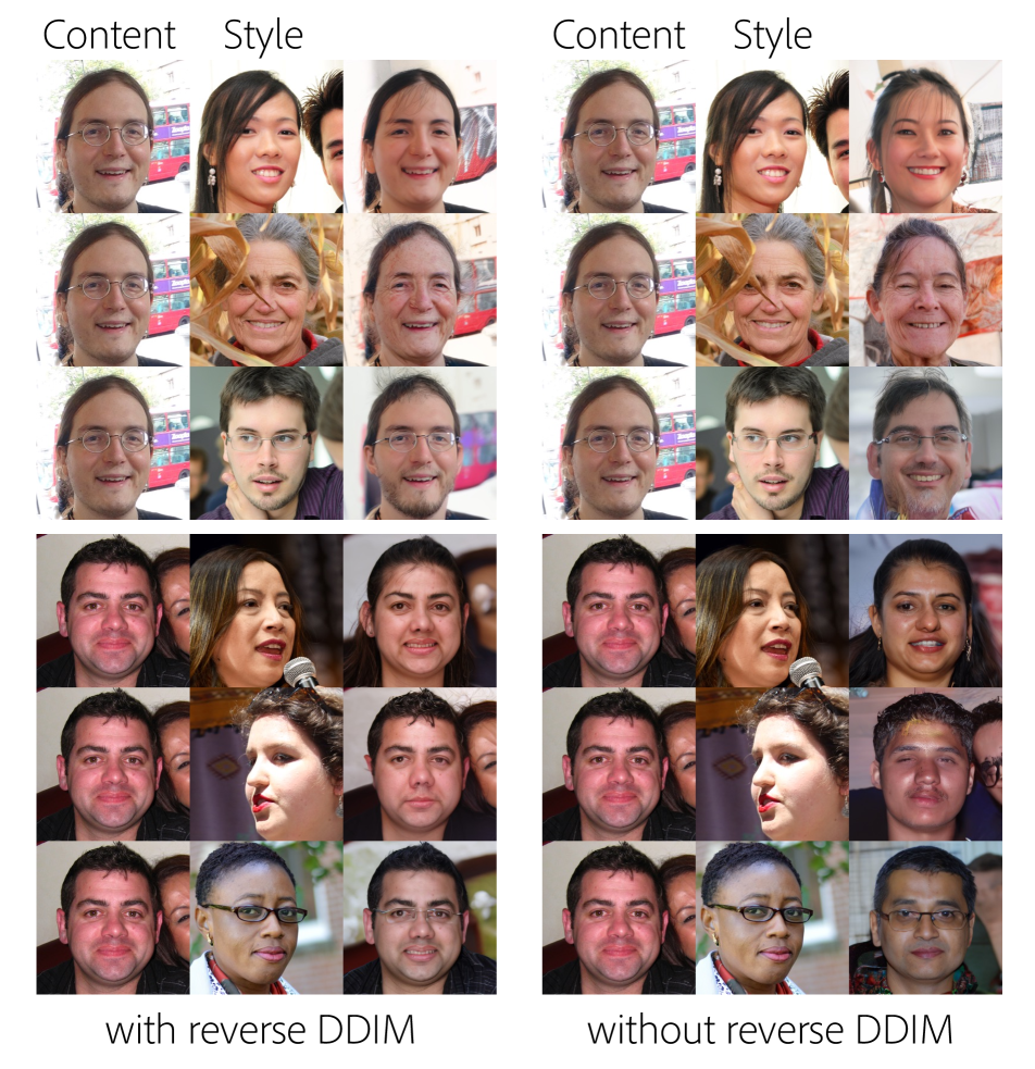
Figure 12: Comparisons between with and without DDIM reverse sampling method in FFHQ dataset.

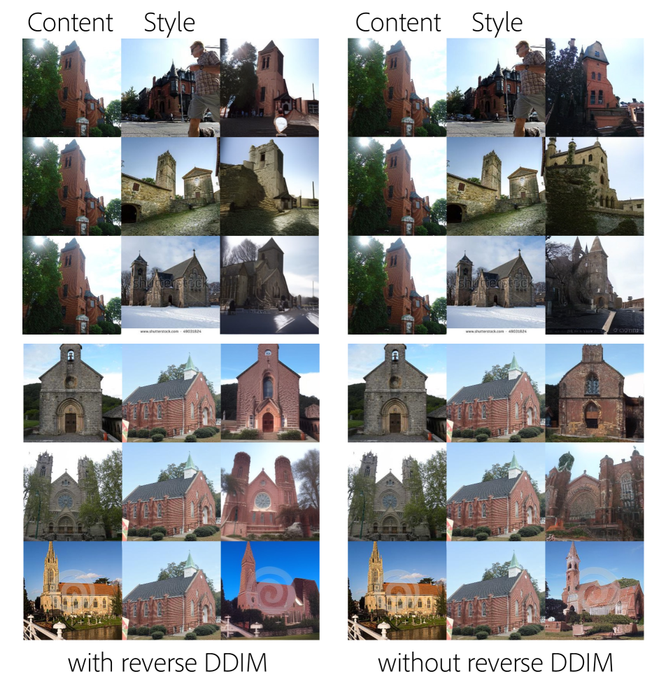
Figure 13: Comparisons between with and without DDIM reverse sampling method in LSUN-church dataset.

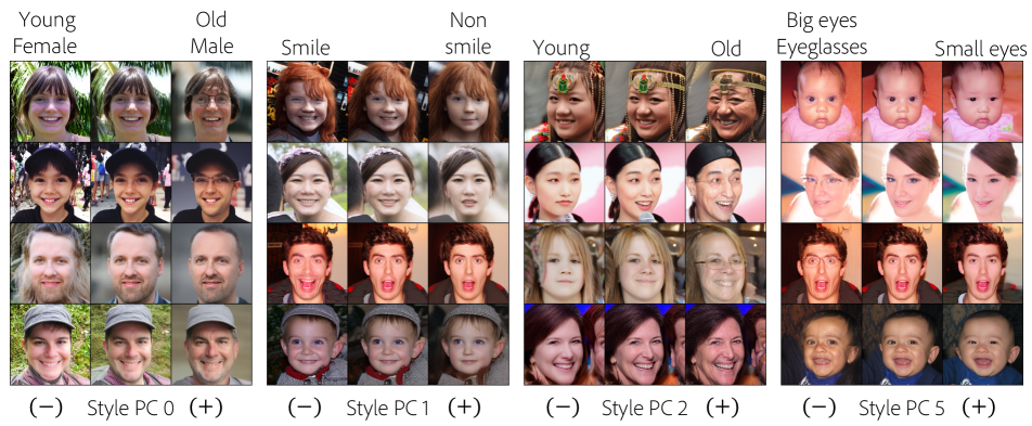
Figure 14: Example image manipulation results on FFHQ dataset by altering the style code learned by the proposed model. We can observe that each PCA component obtained from the style latent code control interpretable, meaningful semantic factors of an image such as smiling, age, gender, hair color and texture, accessories etc. The text above each block describes the attribute being modified while the bottom text refers to the principal component that causes the observed changes. Zoom in for better visibility.

Appendix E Extent of Controllability

In this Section, we present rich controllability of our proposed framework. The latent space exploration is presented in Section E.1. Interpolation results are shown in Section E.2. Further analysis on the latent space is reported in Section E.3.

E.1 Image Manipulation with Latent Space Exploration

One of the advantages of the regularity of GAN latent space is the ability to find directions corresponding to specific attributes of an image that can be used for image manipulation. For example, [15] proposed to use the eigenvectors corresponding to the top principal components of the latent space to manipulate specific attributes. There are also other ways to find meaningful edit directions such as perturbing the dimensions corresponding to style vectors in StyleGAN [50] or using classifiers to find editable directions [23]. DiffAE [40] also used classifiers to find editable directions in their semantic space.

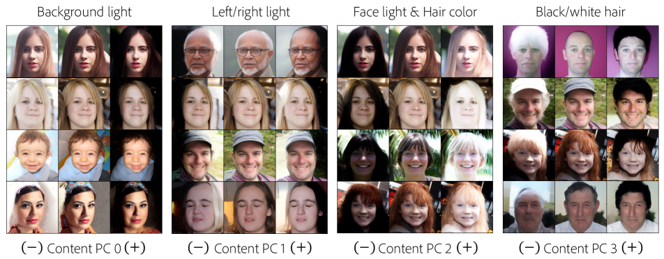
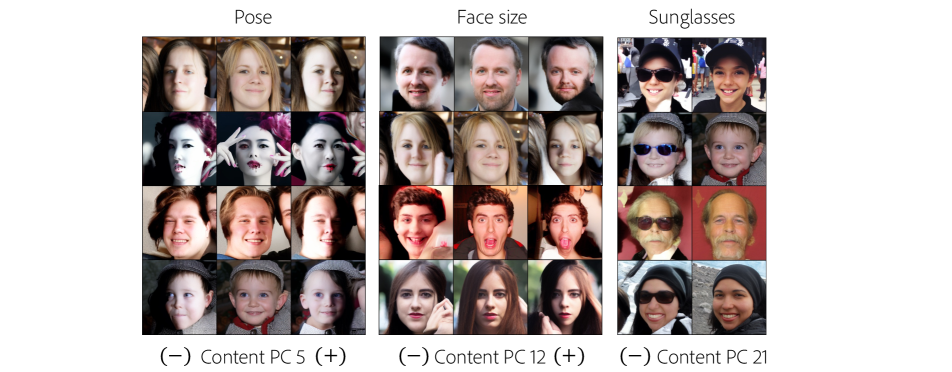
Figure 15: Example image manipulation results on FFHQ dataset by manipulating the content code learned by the proposed model. The components from content code shows controls that correspond to spatial attributes such as pose, lighting and background. The text above each block describes the attribute being modified while the bottom text refers to the principal component that causes the observed changes. Zoom in for better visibility.

To test the regularity and editability of the style and content latent spaces of the proposed model, we apply similar PCA [15] based techniques. We identify that the style codes control semantic information and the top principal components correspond to different attributes that can be seamlessly manipulated. We apply PCA algorithm on the style code $z_{s}$ and the content code $z_{c}$ of all the training images (60000) to get the top 30 Eigenvectors $\mathbf{V_{style}}=\{v_{style}^{0},...,v_{style}^{29}\}$ and $\mathbf{V_{content}}=\{v_{content}^{0},...,v_{content}^{29}\}$. The obtained basis vectors are used for shifting each individual sample.

To manipulate the attribute controlled by the style principal component (PC) on an image I, we pass the content code $z_{c}^{I}$, style code of the same image modified as $z_{s}^{\prime I}=z_{s}^{I}+w_{s}\cdot v_{style}^{0}$ and the noise $x_{T}$ obtained by applying reverse DDIM with content image, for generation. Similar procedure is followed for the content code as well. Please note that PCs are obtained from the training samples while unseen data is taken as input I for the PC experiments.

We performed the analysis with FFHQ and LSUN-church dataset. In FFHQ results, as shown in Fig.14, we observe that the PCs of the style space contain meaningful high-level semantics. For example, the first PC $v_{style}^{0}$ controls gender and age. This indicates that the style encoder learns as intended under our proposed framework. Example generations for $w_{s}\in\{-3,0,3\}$ are shown for various PCs. Fig. 15 shows the results of manipulating the content codes in FFHQ dataset. Interestingly, the content PCs encode the spatial-relevant information, such as the light in the background, light on the left and right, pose, and facial shape. For the content PC experiments, $w_{c}\in\{-1,0,1\}$ is used.

We also explored the same experiments with LSUN-church dataset. Since the foreground region of LSUN-church is not as simple and consistent as that of FFHQ dataset, the content PC results are not consistent. However, we could find some meaningful style PCs because it is designed to contain global features. As seen in Fig. 16 design, texture, abstraction, color are some attributes that are controllable. Images are obtained with $w_{s}\in\{-2,0,2\}$. We believe that using classifiers can possibly lead to better directions for manipulation but it is interesting that simpler PCA based technique provide meaningful semantic edit directions.

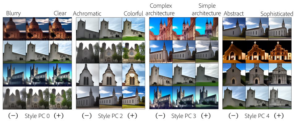
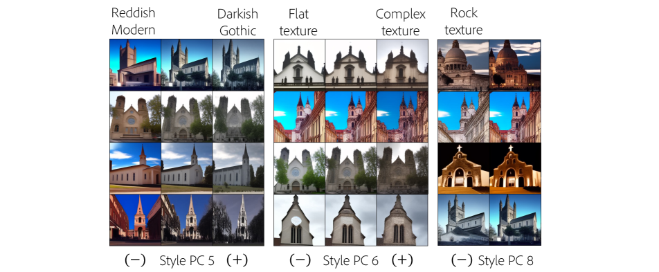
Figure 16: Example image manipulation results on LSUN church dataset by altering the style code learned by the proposed model. We can observe that each PCA component obtained from the style latent code control interpretable, meaningful semantic factors of an image such as texture, color, abstraction and design. The text above each block describes the attribute being modified while the bottom text refers to the principal component that causes the observed changes. Zoom in for better visibility.

E.2 Interpolation

We conducted experiments on the latent space interpolation in order to analyze the effects of the content, the style, and $x_{T}$ during the sampling process. All the results use reverse DDIM with content image to get $x_{T}$ that is used during sampling.

Fig. 17 shows the content-only interpolation results where style code $z_{s}$ and noise $x_{T}$ are fixed to the image in the first column. The gray box on the top indicates the fixed input while $z_{c}$ is interpolated between the two images in the first two columns. From the figure, we can see that the style information and the person identity are maintained while pose and facial shape are changed.

Fig. 18 shows the case $x_{T}$ obtained from reverse DDIM of the images in the first two columns is interpolated while the style and content features are fixed to the image in the first column. The content (e.g., pose, facial shape) and the style (e.g., beard, eyeglasses, and facial color) are maintained while stochastic properties change. We can see that identity is not entirely tied to $x_{T}$ but the stochastic changes to cause change in the identity. This is why using reverse DDIM to fix $x_{T}$ preserves better identity.

Fig. 19 visualizes the style interpolation while content and $x_{t}$ are fixed to the first image. The person identity, the pose and facial shape are preserved while the facial expression, gender, and age are smoothly changed validating our results.

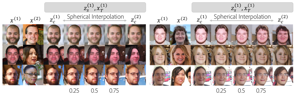
Figure 17: Content interpolation results. Style and $x_{T}$ are obtained from images in the first column while content code is interpolated between images in column 1 and column 2. We can see how content specific factors vary smoothly.

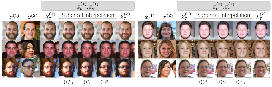
Figure 18: $x_{T}$ interpolation results where style and content are obtained from images in the first column while $x_{T}$ is interpolated between reverse DDIM of both images. We can see stochastic changes causing mild identity changes. Fixing $x_{T}$ to the content image hence provides better identity preservation for image translation and manipulation.

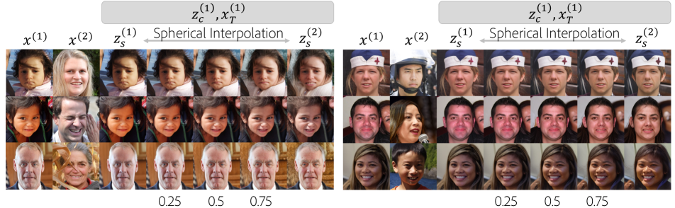
Figure 19: Style interpolation results when content and $x_{T}$ are obtained from images in the first column. We can see smooth changes in the semantic attributes such as age, gender, smile, eyeglasses etc. allowing for effective style manipulations.

E.3 Interpreting the Latent Spaces

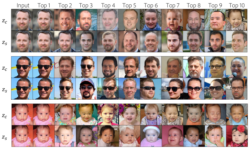
Figure 20: KNN results of the content and the style features showing what semantic attributes content and style codes encode.

We additionally perform K Nearest Neighbor (KNN) experiments to understand what features are encoded in the content and style latent representations. We pass 10000 unseen images through the style and the content encodersto get $z_{c}$ and $z_{s}$. We then compute the distance of an arbitrary sample with the entire validation set and sort the 10000 distances.

The results are shown in Fig. 20 and Fig. 21. The first column denotes the input image while the rest of the columns shows the top 10 images that have the closest content or style features indicated by $z_{c}$ (first row within each macro row) and $z_{s}$ (second row within each macro row) respectively. The second column is the same image. We can see that the content feature mainly contains the pose and the facial shape information while the style has the high-level semantics, such as wearing eyeglasses, gender, age, accessories, and hair color.

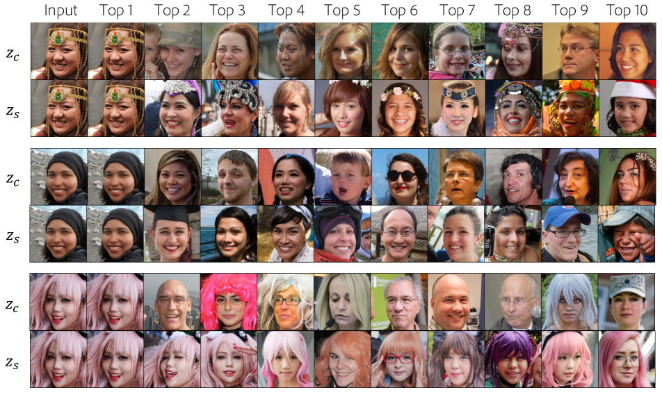
Figure 21: KNN results of the content and the style features showing what semantic attributes content and style codes encode.

Appendix F Timestep Scheduling

F.1 Training an Implicit Mixture-Of-Experts

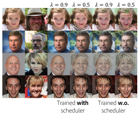
Figure 22: Effects of using the proposed timestep scheduling in training.

Our timestep scheduling approach proposed in Sec 3.2 in the main paper was applied only during sampling for results in the main paper. We trained a model with timestep scheduling applied during training to analyze how it affects the behavior of our framework. Fig. 22 shows the comparisons between the models trained with and without the scheduler. For the results trained with scheduler, we used $a=0.1$ and $b=529$ ($\text{SNR}^{-1}(0.1)$) for both training and sampling. As can be seen in the rightmost two columns, the style effects are relatively small although given $\lambda$ is controlled. It is because the style encoder is trained to be injected only in the early timesteps (0-528), which makes the style representations learn limited features (e.g., eyeglasses are not encoded in the style, as shown in the second row). However, we observe better decomposition between factors controlled by content and style compared to using the timestep scheduling only during sampling. We believe this is because, using timestep scheduling to vary the conditioning input at each timestep implicitly trains the model to specialize to the varied conditioning, implictly learing a mixture–of–experts like model [1]. We believe this could be a promising avenue for future research to train expert models without maintaining different entirely finetuned models and leave further analysis as future work.

F.2 Experiment with different timestep schedules

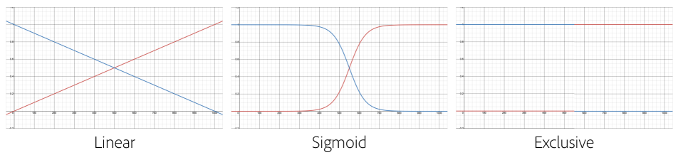
Figure 23: Plots for different timestep scheduling strategies. The illustrated plot of the sigmoid scheduler is from $a=0.025$ and $b=550$. Bigger $a$ makes it similar to the exclusive scheduler while smaller $a$ makes it close to the linear scheduler. The blue line indicates the weight scheduler for the style and the red line is for the content.

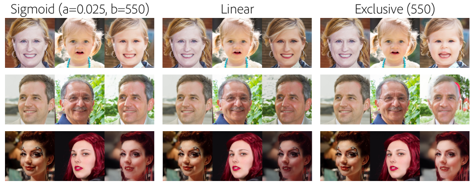
Figure 24: Comparison between different timestep scheduled during sampling. Sigmoid has a softer schedule with more controllability and thus results is more natural generations compared to the other techniques.

We compare the different timestep schedulers illustrated in Fig. 23 during sampling. Note that these schedules are not used for training. In the exclusive scheduling, the style weight is one if $t\leq 550$ and zero otherwise. The content weight is applied when style weight is not applied. In the linear scheduling, the style weight linearly decreases from $1$ at $t=0$ to $0$ at $t=999$ while the content weight increases linearly from $0$ to $1$. The sigmoid scheduling is the one propose in Eq. 2 and 3.

The comparison results are shown in Fig. 24. We can observe that the exclusive scheduling shows either magnified style or unnatural generations compared to the sigmoid scheduling. Since it is difficult to exactly define the role of each timestep, naively separating the point where to exclusively apply content and style yields the undesirable results. The linear schedule does not work for all images and has limited control. However, the sigmoid scheduling provides a softer weighting scheme leading to better generations and has additional controls to get desired results.

Appendix G Additional Results

In this Section, we provide additional results of our proposed framework. Fig. 25 shows example generations using CDM and GCDM from the same model. CDM consistently shows two failure modes specific to reference based image translation. First, content-style overlap showing that content and style codes have certain common information that is not further disentangled during sampling (e.g., first and second rows in the figure). Next is unnatural generation (e.g., third and fourth rows) where the generated images do not look realistic enough.

Fig. 26 shows the additional results on FFHQ dataset. Fig. 27 shows the results of multiple style and single content, and vice versa on LSUN church dataset. Fig. 28 shows the hyperparameters used for CDM and GCDM on Stable Diffusion V2.

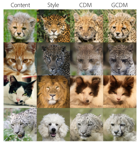
Figure 25: Comparisons between GCDM and CDM demonstrating that CDM can output unnatural images while GCDM can generate realistic images. We use DDIM [47] sampler, and the reverse process is done from $T=600$ inspired by SDEdit [37]. $z_{600}$ is obtained by $q(z_{600}|E_{LDM}(x_{c}))$ using the content image. $x_{T}$ is randomly sampled.

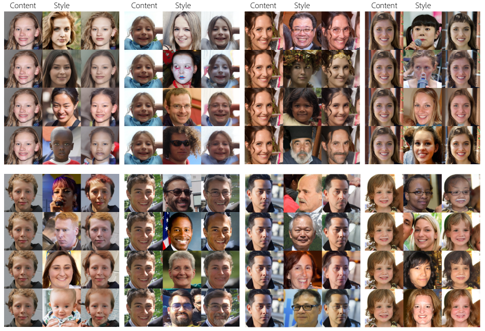
Figure 26: Additional results on FFHQ. The results are sampled by reverse DDIM.

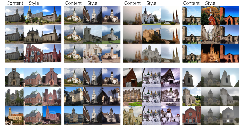
Figure 27: Additional results on LSUN-church. The results are sampled by reverse DDIM.

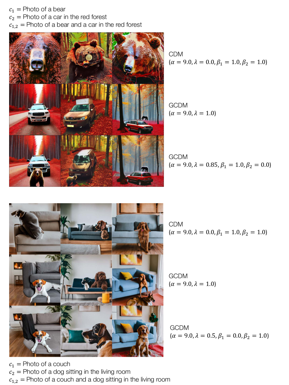
Figure 28: Text2image synthesis results with GCDM hyperparameters.

References

- [1] Yogesh Balaji, Seungjun Nah, Xun Huang, Arash Vahdat, Jiaming Song, Karsten Kreis, Miika Aittala, Timo Aila, Samuli Laine, Bryan Catanzaro, et al. ediffi: Text-to-image diffusion models with an ensemble of expert denoisers. arXiv preprint arXiv:2211.01324, 2022.
- [2] Diane Bouchacourt, Ryota Tomioka, and Sebastian Nowozin. Multi-level variational autoencoder: Learning disentangled representations from grouped observations. In Proceedings of the AAAI Conference on Artificial Intelligence, volume 32, 2018.
- [3] Mathilde Caron, Hugo Touvron, Ishan Misra, Hervé Jégou, Julien Mairal, Piotr Bojanowski, and Armand Joulin. Emerging properties in self-supervised vision transformers. In Proceedings of the International Conference on Computer Vision (ICCV), 2021.
- [4] Wonwoong Cho, Sungha Choi, David Keetae Park, Inkyu Shin, and Jaegul Choo. Image-to-image translation via group-wise deep whitening-and-coloring transformation. In Proceedings of the IEEE/CVF Conference on Computer Vision and Pattern Recognition, pages 10639–10647, 2019.
- [5] Jooyoung Choi, Sungwon Kim, Yonghyun Jeong, Youngjune Gwon, and Sungroh Yoon. Ilvr: Conditioning method for denoising diffusion probabilistic models. arXiv preprint arXiv:2108.02938, 2021.
- [6] Jooyoung Choi, Jungbeom Lee, Chaehun Shin, Sungwon Kim, Hyunwoo Kim, and Sungroh Yoon. Perception prioritized training of diffusion models. In Proceedings of the IEEE/CVF Conference on Computer Vision and Pattern Recognition, pages 11472–11481, 2022.
- [7] Yunjey Choi, Youngjung Uh, Jaejun Yoo, and Jung-Woo Ha. Stargan v2: Diverse image synthesis for multiple domains. In Proceedings of the IEEE/CVF conference on computer vision and pattern recognition, pages 8188–8197, 2020.
- [8] Prafulla Dhariwal and Alexander Nichol. Diffusion models beat gans on image synthesis. Advances in Neural Information Processing Systems, 34:8780–8794, 2021.
- [9] Prafulla Dhariwal and Alexander Nichol. Diffusion models beat gans on image synthesis. In M. Ranzato, A. Beygelzimer, Y. Dauphin, P.S. Liang, and J. Wortman Vaughan, editors, Advances in Neural Information Processing Systems, volume 34, pages 8780–8794. Curran Associates, Inc., 2021.
- [10] Laurent Dinh, Jascha Sohl-Dickstein, and Samy Bengio. Density estimation using real NVP. In International Conference on Learning Representations, 2017.
- [11] Patrick Esser, Robin Rombach, and Bjorn Ommer. A disentangling invertible interpretation network for explaining latent representations. In Proceedings of the IEEE/CVF Conference on Computer Vision and Pattern Recognition (CVPR), June 2020.
- [12] Patrick Esser, Robin Rombach, and Bjorn Ommer. Taming transformers for high-resolution image synthesis. In Proceedings of the IEEE/CVF conference on computer vision and pattern recognition, pages 12873–12883, 2021.
- [13] Rinon Gal, Yuval Alaluf, Yuval Atzmon, Or Patashnik, Amit H Bermano, Gal Chechik, and Daniel Cohen-Or. An image is worth one word: Personalizing text-to-image generation using textual inversion. arXiv preprint arXiv:2208.01618, 2022.
- [14] Ian Goodfellow, Jean Pouget-Abadie, Mehdi Mirza, Bing Xu, David Warde-Farley, Sherjil Ozair, Aaron Courville, and Yoshua Bengio. Generative adversarial nets. In Z. Ghahramani, M. Welling, C. Cortes, N. Lawrence, and K.Q. Weinberger, editors, Advances in Neural Information Processing Systems, volume 27. Curran Associates, Inc., 2014.
- [15] Erik Härkönen, Aaron Hertzmann, Jaakko Lehtinen, and Sylvain Paris. Ganspace: Discovering interpretable gan controls. Advances in Neural Information Processing Systems, 33:9841–9850, 2020.
- [16] Amir Hertz, Ron Mokady, Jay Tenenbaum, Kfir Aberman, Yael Pritch, and Daniel Cohen-Or. Prompt-to-prompt image editing with cross attention control. arXiv preprint arXiv:2208.01626, 2022.
- [17] Martin Heusel, Hubert Ramsauer, Thomas Unterthiner, Bernhard Nessler, and Sepp Hochreiter. Gans trained by a two time-scale update rule converge to a local nash equilibrium. Advances in neural information processing systems, 30, 2017.
- [18] Jonathan Ho, Ajay Jain, and Pieter Abbeel. Denoising diffusion probabilistic models. Advances in Neural Information Processing Systems, 33:6840–6851, 2020.
- [19] Jonathan Ho and Tim Salimans. Classifier-free diffusion guidance. arXiv preprint arXiv:2207.12598, 2022.
- [20] Judy Hoffman, Eric Tzeng, Taesung Park, Jun-Yan Zhu, Phillip Isola, Kate Saenko, Alexei Efros, and Trevor Darrell. Cycada: Cycle-consistent adversarial domain adaptation. In International conference on machine learning, pages 1989–1998. Pmlr, 2018.
- [21] Xun Huang, Ming-Yu Liu, Serge Belongie, and Jan Kautz. Multimodal unsupervised image-to-image translation. In Proceedings of the European conference on computer vision (ECCV), pages 172–189, 2018.
- [22] Tero Karras, Samuli Laine, and Timo Aila. A style-based generator architecture for generative adversarial networks. In Proceedings of the IEEE/CVF conference on computer vision and pattern recognition, pages 4401–4410, 2019.
- [23] Tero Karras, Samuli Laine, Miika Aittala, Janne Hellsten, Jaakko Lehtinen, and Timo Aila. Analyzing and improving the image quality of StyleGAN. In Proc. CVPR, 2020.
- [24] Bahjat Kawar, Shiran Zada, Oran Lang, Omer Tov, Huiwen Chang, Tali Dekel, Inbar Mosseri, and Michal Irani. Imagic: Text-based real image editing with diffusion models. arXiv preprint arXiv:2210.09276, 2022.
- [25] Gwanghyun Kim, Taesung Kwon, and Jong Chul Ye. Diffusionclip: Text-guided diffusion models for robust image manipulation. In Proceedings of the IEEE/CVF Conference on Computer Vision and Pattern Recognition, pages 2426–2435, 2022.
- [26] Diederik Kingma, Tim Salimans, Ben Poole, and Jonathan Ho. Variational diffusion models. In M. Ranzato, A. Beygelzimer, Y. Dauphin, P.S. Liang, and J. Wortman Vaughan, editors, Advances in Neural Information Processing Systems, volume 34, pages 21696–21707. Curran Associates, Inc., 2021.
- [27] Diederik P Kingma and Max Welling. Auto-encoding variational bayes. arXiv preprint arXiv:1312.6114, 2013.
- [28] Zhifeng Kong and Wei Ping. On fast sampling of diffusion probabilistic models. In ICML Workshop on Invertible Neural Networks, Normalizing Flows, and Explicit Likelihood Models, 2021.
- [29] Gihyun Kwon and Jong Chul Ye. Diagonal attention and style-based gan for content-style disentanglement in image generation and translation. In Proceedings of the IEEE/CVF International Conference on Computer Vision, pages 13980–13989, 2021.
- [30] Gihyun Kwon and Jong Chul Ye. Diffusion-based image translation using disentangled style and content representation. arXiv preprint arXiv:2209.15264, 2022.
- [31] Oran Lang, Yossi Gandelsman, Michal Yarom, Yoav Wald, Gal Elidan, Avinatan Hassidim, William T Freeman, Phillip Isola, Amir Globerson, Michal Irani, et al. Explaining in style: Training a gan to explain a classifier in stylespace. In Proceedings of the IEEE/CVF International Conference on Computer Vision, pages 693–702, 2021.
- [32] Hsin-Ying Lee, Hung-Yu Tseng, Jia-Bin Huang, Maneesh Singh, and Ming-Hsuan Yang. Diverse image-to-image translation via disentangled representations. In Proceedings of the European conference on computer vision (ECCV), pages 35–51, 2018.
- [33] Jun Hao Liew, Hanshu Yan, Daquan Zhou, and Jiashi Feng. Magicmix: Semantic mixing with diffusion models. arXiv preprint arXiv:2210.16056, 2022.
- [34] Nan Liu, Shuang Li, Yilun Du, Antonio Torralba, and Joshua B Tenenbaum. Compositional visual generation with composable diffusion models. Proceedings of the European conference on computer vision (ECCV), 2022.
- [35] Cheng Lu, Yuhao Zhou, Fan Bao, Jianfei Chen, Chongxuan Li, and Jun Zhu. DPM-solver: A fast ODE solver for diffusion probabilistic model sampling in around 10 steps. In Alice H. Oh, Alekh Agarwal, Danielle Belgrave, and Kyunghyun Cho, editors, Advances in Neural Information Processing Systems, 2022.
- [36] Cheng Lu, Yuhao Zhou, Fan Bao, Jianfei Chen, Chongxuan Li, and Jun Zhu. Dpm-solver++: Fast solver for guided sampling of diffusion probabilistic models. arXiv preprint arXiv:2211.01095, 2022.
- [37] Chenlin Meng, Yutong He, Yang Song, Jiaming Song, Jiajun Wu, Jun-Yan Zhu, and Stefano Ermon. Sdedit: Guided image synthesis and editing with stochastic differential equations. In International Conference on Learning Representations, 2021.
- [38] Alexander Quinn Nichol and Prafulla Dhariwal. Improved denoising diffusion probabilistic models. In International Conference on Machine Learning, pages 8162–8171. PMLR, 2021.
- [39] Taesung Park, Jun-Yan Zhu, Oliver Wang, Jingwan Lu, Eli Shechtman, Alexei Efros, and Richard Zhang. Swapping autoencoder for deep image manipulation. Advances in Neural Information Processing Systems, 33:7198–7211, 2020.
- [40] Konpat Preechakul, Nattanat Chatthee, Suttisak Wizadwongsa, and Supasorn Suwajanakorn. Diffusion autoencoders: Toward a meaningful and decodable representation. In Proceedings of the IEEE/CVF Conference on Computer Vision and Pattern Recognition, pages 10619–10629, 2022.
- [41] Aditya Ramesh, Prafulla Dhariwal, Alex Nichol, Casey Chu, and Mark Chen. Hierarchical text-conditional image generation with clip latents, 2022.
- [42] Robin Rombach, Andreas Blattmann, Dominik Lorenz, Patrick Esser, and Björn Ommer. High-resolution image synthesis with latent diffusion models. In Proceedings of the IEEE/CVF Conference on Computer Vision and Pattern Recognition, pages 10684–10695, 2022.
- [43] Olaf Ronneberger, Philipp Fischer, and Thomas Brox. U-net: Convolutional networks for biomedical image segmentation. In International Conference on Medical image computing and computer-assisted intervention, pages 234–241. Springer, 2015.
- [44] Nataniel Ruiz, Yuanzhen Li, Varun Jampani, Yael Pritch, Michael Rubinstein, and Kfir Aberman. Dreambooth: Fine tuning text-to-image diffusion models for subject-driven generation. 2022.
- [45] Chitwan Saharia, William Chan, Saurabh Saxena, Lala Li, Jay Whang, Emily Denton, Seyed Kamyar Seyed Ghasemipour, Burcu Karagol Ayan, S. Sara Mahdavi, Rapha Gontijo Lopes, Tim Salimans, Jonathan Ho, David J Fleet, and Mohammad Norouzi. Photorealistic text-to-image diffusion models with deep language understanding, 2022.
- [46] Jascha Sohl-Dickstein, Eric Weiss, Niru Maheswaranathan, and Surya Ganguli. Deep unsupervised learning using nonequilibrium thermodynamics. In International Conference on Machine Learning, pages 2256–2265. PMLR, 2015.
- [47] Jiaming Song, Chenlin Meng, and Stefano Ermon. Denoising diffusion implicit models. In International Conference on Learning Representations, 2020.
- [48] Narek Tumanyan, Omer Bar-Tal, Shai Bagon, and Tali Dekel. Splicing vit features for semantic appearance transfer. In Proceedings of the IEEE/CVF Conference on Computer Vision and Pattern Recognition, pages 10748–10757, 2022.
- [49] Dani Valevski, Matan Kalman, Yossi Matias, and Yaniv Leviathan. Unitune: Text-driven image editing by fine tuning an image generation model on a single image. arXiv preprint arXiv:2210.09477, 2022.
- [50] Zongze Wu, Dani Lischinski, and Eli Shechtman. Stylespace analysis: Disentangled controls for stylegan image generation. In Proceedings of the IEEE/CVF Conference on Computer Vision and Pattern Recognition, pages 12863–12872, 2021.
- [51] Zhisheng Xiao, Karsten Kreis, and Arash Vahdat. Tackling the generative learning trilemma with denoising diffusion GANs. In International Conference on Learning Representations, 2022.
- [52] Fisher Yu, Ari Seff, Yinda Zhang, Shuran Song, Thomas Funkhouser, and Jianxiong Xiao. Lsun: Construction of a large-scale image dataset using deep learning with humans in the loop. arXiv preprint arXiv:1506.03365, 2015.
- [53] Jiahui Yu, Yuanzhong Xu, Jing Yu Koh, Thang Luong, Gunjan Baid, Zirui Wang, Vijay Vasudevan, Alexander Ku, Yinfei Yang, Burcu Karagol Ayan, Ben Hutchinson, Wei Han, Zarana Parekh, Xin Li, Han Zhang, Jason Baldridge, and Yonghui Wu. Scaling autoregressive models for content-rich text-to-image generation, 2022.