One-Shot Video Inpainting
Abstract
Recently, removing objects from videos and filling in the erased regions using deep video inpainting (VI) algorithms has attracted considerable attention. Usually, a video sequence and object segmentation masks for all frames are required as the input for this task. However, in real-world applications, providing segmentation masks for all frames is quite difficult and inefficient. Therefore, we deal with VI in a one-shot manner, which only takes the initial frame’s object mask as its input. Although we can achieve that using naive combinations of video object segmentation (VOS) and VI methods, they are sub-optimal and generally cause critical errors. To address that, we propose a unified pipeline for one-shot video inpainting (OSVI). By jointly learning mask prediction and video completion in an end-to-end manner, the results can be optimal for the entire task instead of each separate module. Additionally, unlike the two-stage methods that use the predicted masks as ground truth cues, our method is more reliable because the predicted masks can be used as the network’s internal guidance. On the synthesized datasets for OSVI, our proposed method outperforms all others both quantitatively and qualitatively.
1 Introduction
Video inpainting (VI) is a task that aims to remove a designated object in a given video sequence and fill in that area with plausible content. General approaches for VI take a video sequence and object segmentation masks for all frames as their input. However, in real-world applications, obtaining object segmentation masks for every frame is usually difficult and labor-intensive. To address this issue, we expand on an approach that is better suited to practical scenarios, namely one-shot video inpainting (OSVI). Compared to a conventional VI that requires full-frame segmentation masks as shown in Figure 1 (a), OSVI requires only the initial frames’s object mask and internally predicts those of subsequent frames while filling the missing content for all frames; this is depicted in Figure 1 (b).
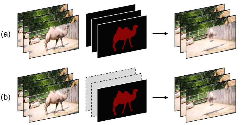
OSVI can be achieved by sequentially connecting a video object segmentation (VOS) network and a VI network as a two-stage pipeline. Using the initial frame object annotation, the VOS network first generates that object’s entire frame masks. Then, using full-frame object masks as its input, the VI network fills in the object regions with plausible content that befits the background. However, this two-stage approach suffers from critical issues when directly applied to OSVI. Here, we will discuss this approach’s two main problems. First, since the entire network is not trained in an end-to-end manner, the results are optimal for each separate module but not as a whole. This property that two different networks are trained based on respective objectives leads to sub-optimal results for OSVI. Second, existing VI algorithms assume that the object masks received as input are always accurate. Therefore, if the predicted masks generated from a VOS model, which could be inaccurate, are provided as their input, the system will severely break down. This phenomenon will be particularly more drastic for flow-based VI methods where reference pixels are directly warped to the target region.
To address these concerns, we propose an end-to-end learnable baseline network that consists of mask prediction and video completion modules sharing a single encoder’s embedded features. Unlike existing VI algorithms, we erase the object region at the feature level by adopting a novel transformer architecture. Our proposed method demonstrates its effectiveness for OSVI on synthetic datasets both quantitatively and qualitatively. Compared with two-stage methods, which are mainly naive combinations of existing VOS and VI methods, our method surpasses all of them by a large margin.
Our main contributions can be summarized as follows:
-
•
We expand VI to OSVI, which refers to erasing a designated object in a video sequence only using a single frame annotation.
-
•
We propose a novel end-to-end learnable algorithm that can handle OSVI more effectively when compared to existing two-stage approaches.
-
•
Our proposed method outperforms all existing methods on synthetic datasets.
2 Related Work
Object removal. Due to its usefulness in diverse vision applications, such as video editing, object removal has been of interest recently. Shetty et al. (Shetty, Fritz, and Schiele 2018) propose a GAN-based two-stage network composed of a mask generator and an image inpainter for object removal in an image. DynaFill (Bešić and Valada 2020) presents a new type of network using depth completion on the inpainted image. The depth map predicted from the inpainted image of a previous frame is used as guidance for current frame image inpainting. AutoRemover (Zhang et al. 2020) takes masks as its input and detects shadows using them. By using object masks and extracted shadow masks, the network can erase their shadows as well as objects in a video. VORNet (Chang, Yu Liu, and Hsu 2019) fills the missing object regions only with box annotations as weak supervision to reduce annotation efforts.
Video object segmentation. Semi-supervised VOS is a pixel-level classification task that tracks and segments an arbitrary target object in a video. To efficiently handle an arbitrary target object, early works, such as OSVOS (Caelles et al. 2017), OnAVOS (Voigtlaender and Leibe 2017) and OSVOS-S (Maninis et al. 2018), are based on online learning that trains a network during test time. However, since online learning is impractical for real-world applications because of its huge computational cost at test time, recent methods are based on feature matching that compares query frame features to reference frame features without online learning. VideoMatch (Hu, Huang, and Schwing 2018) extracts features from an initial frame and a query frame and then matches them at pixel-level using a soft matching layer. FEELVOS (Voigtlaender et al. 2019) extends the use of pixel-level matching by employing initial and previous frames as reference ones; it also uses the matching output as the network’s internal guidance. CFBI (Yang, Wei, and Yang 2020) improves FEELVOS by employing background matching as well as foreground matching. To fully utilize the information from all past frames as well as initial and previous frames, STM (Oh et al. 2019a) proposes the space–time memory network, in which query frame features are densely matched to the memory features built from all past frames, covering all space–time locations. AFB-URR (Liang et al. 2020) and XMem (Cheng and Schwing 2022) improves the memory construction scheme to design a model robust to long videos.
Video inpainting. Early works (Huang et al. 2016; Wexler, Shechtman, and Irani 2004) use patch-based optimization to restore missing regions with valid regions for VI. However, these methods have some limitations. For example, they face difficulty in representing dynamic motions while maintaining temporal consistency, in addition to requiring high computational costs. To address these issues, various deep learning-based methods have been proposed within the past few years. These studies can be divided into two categories: patch-based approaches (Lee et al. 2019; Oh et al. 2019b; Zeng, Fu, and Chao 2020; Li et al. 2020; Liu et al. 2021) and flow-based approaches (Kim et al. 2019; Xu et al. 2019; Gao et al. 2020; Zou et al. 2021; Li et al. 2022). Patch-based approaches aim to fill missing regions using direct pixel-level feature matching. CPNet (Lee et al. 2019) uses an alignment network to fill missing regions by using the different object positions with background matching. OPN (Oh et al. 2019b) proposes a similarity matching network that extracts and compares key and value features for each frame. It also suggests a post-processing network called the TCN, which uses a recurrent structure to increase temporal consistency. STTN (Zeng, Fu, and Chao 2020) is composed of an encoder–decoder architecture and multi-layer multi-head spatio-temporal transformers trained using a 3D discriminator for temporal consistency. BSCA (Li et al. 2020) proposes a boundary-aware short-term module for adjacent frame matching and a dynamic long-term context aggregation module for temporal consistency. FuseFormer (Liu et al. 2021) develops the transformer-based algorithms by proposing a method of efficiency patch splitting and composing. By contrast, flow-based approaches exploit the optical flow map for VI. VINet (Kim et al. 2019) proposes a flow warping-based recurrent network that refers to adjacent frames. DFVI (Xu et al. 2019) restores flow maps extracted using a pre-trained flow estimation network by performing forward–backward pixel propagation. FGVC (Gao et al. 2020) presents a flow–edge completion technique for the sharpness of flow map edges, a color propagation in the gradient domain for reducing warping error, and a non-local flow to resolve the chronic problem of flow maps; the latter namely being that they cannot obtain clearness when adjacent frames lack in information. TSAM (Zou et al. 2021) proposes a method that applies flow warping to the feature level based on the DNN architecture. E2FGVI (Li et al. 2022) shows the problems of previous flow-based pipelines and solves them by presenting the unified pipeline in an end-to-end manner.
3 Proposed Approach
3.1 Problem Formulation
Let us denote a video as , ground truth object masks as , and a ground truth clean video as . Our goal is to generate the predicted object masks and clean video , where and are provided as input.
3.2 Network Overview
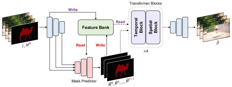
An overview of our proposed network is shown in Figure 2. It consists of two modules, a mask prediction module and a video completion module. First, the mask prediction module predicts the segmentation masks for all frames using the segmentation mask from the initial frame and the features extracted from each frame. The predicted masks and the extracted features are stored in a feature bank for reuse. As the semantic cues obtained from the mask prediction module are transferred to the video completion module without gradient disconnection, the entire network can be trained in an end-to-end manner.
3.3 Mask Prediction Module
Memory construction. To propagate the object information of the initial frame, i.e., ground truth segmentation mask, we employ a memory-based architecture as in STM (Oh et al. 2019a). From , we first extract base features . Then, key features and value features can be obtained as
| (1) | |||
| (2) |
where and indicate channel concatenation and adaptive spatial pooling, respectively. The extracted key and value features are then stored in memory to be used for future frame prediction.
One of the memory architecture’s main advantages is its ability to simultaneously store an arbitrary number of frames in memory. To fully exploit dense cues of a video, we store the key and value features of every five frames in the memory as well as the initial frame during the inference. Assuming frames are stored in the memory, the memory key and value features can be defined as and , respectively.
Memory read. Based on the accumulated information (memory key and value features) obtained from past frames, the goal is to predict the query frame mask. To this end, we first extract query key features from the query frame image and compare them to memory key features to calculate visual similarity. Then, we transfer the object cues, i.e., the memory value features , to the query frame and the query frame value features can be obtained. This process is identical to popular self-attention mechanism (Vaswani et al. 2017), and can be represented as
| (3) | |||
| (4) |
where and indicate a query-wise softmax operation and matrix multiplication.
Mask prediction. As contains object cues of the query frame, object segmentation masks can be obtained by decoding it. To do that, we gradually increase the spatial size using the low-level features extracted from the encoder via skip connections. To obtain better feature representations, we add a CBAM (Woo et al. 2018) layer after every skip connection.
3.4 Video Completion Module
Masked multi-head attention. In our framework, visual features are extracted from a video sequence and stored in the feature bank to be used for both mask prediction and video completion modules. Unlike conventional VI methods where object features are excluded, the features in our model contain object information since they should also be used to track a designated object. Considering object features may be referenced when filling the missing region, this will severely degrade the performance of the system. To address this issue, we propose a novel masked multi-head attention (MMHA) for transformer architecture.
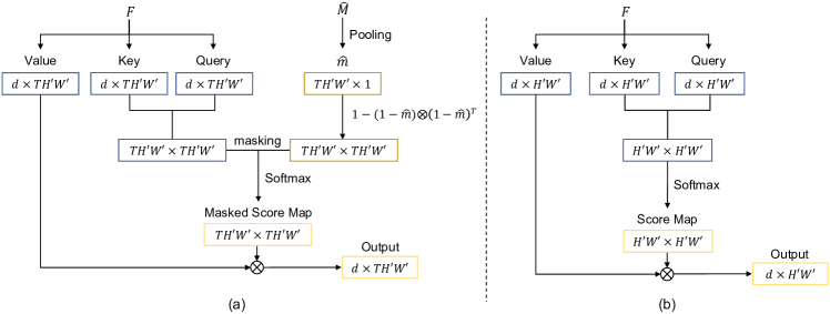
The MMHA’s visualized workflow is shown in Figure 3 (a). Given that represents input features of a transformer block and is a downsampled version of , we can obtain a mask guidance matrix as , after reshaping to . Then, the mask guidance matrix is masked to a key–query similarity map to remove the object region from consideration. However, as a softmax operation comes after this process, we adopt a value substitution operation instead of a simple multiplication. This process can be represented as
| (5) |
where indicates the key–query matching scores. This allows us to diminish the influence of the object regions even after the softmax operation. In summary, the MMHA plays two roles: 1) it prevents object regions from bringing semantic cues from other object regions; 2) it forces object regions not to affect other valid regions by limiting content propagation.
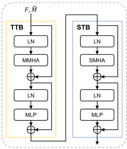
Spatio-temporal transformer. As shown in Figure 4, we divide the general transformer block into a temporal transformer block (TTB) and a spatial transformer block (STB). The architectures of both are identical to that of the general transformer architecture, i.e., the sequential connection of multi-head attention and multi-layer perceptron. However, the TTB exchanges semantic cues between multiple frames, while the STB internally exchanges semantic cues in a single frame. Furthermore, due to the difference in the attention layer, they have different objectives. The TTB is used to erase object cues and fill object regions by leveraging the cues from other frames, while the STB is used to internally fill those regions within a single frame.
Given that is -th features where , and is the number of total transformer blocks, the transformer block formula can be defined as
| (6) | |||
| (7) | |||
| (8) | |||
| (9) |
where and indicate multi-layer perceptron and layer normalization layer (Ba, Kiros, and Hinton 2016), respectively.
| VOS | VI | DAYT | BLDA | ||||
|---|---|---|---|---|---|---|---|
| PSNR | SSIM | LPIPS | PSNR | SSIM | LPIPS | ||
| FRTM | CPNet | 27.038 | 0.9324 | 0.0946 | 29.998 | 0.9644 | 0.0451 |
| STTN | 25.357 | 0.9118 | 0.1032 | 28.167 | 0.9388 | 0.0552 | |
| FGVC | 27.082 | 0.9300 | 0.0922 | 30.114 | 0.9650 | 0.0409 | |
| FuseFormer | 28.495 | 0.9343 | 0.0901 | 34.115 | 0.9661 | 0.0422 | |
| CFBI | CPNet | 31.985 | 0.9591 | 0.0616 | 33.716 | 0.9728 | 0.0336 |
| STTN | 30.388 | 0.9400 | 0.0618 | 31.139 | 0.9477 | 0.0414 | |
| FGVC | 32.124 | 0.9541 | 0.0484 | 34.491 | 0.9749 | 0.0240 | |
| FuseFormer | 34.309 | 0.9623 | 0.0472 | 38.427 | 0.9751 | 0.0282 | |
| BMVOS | CPNet | 31.910 | 0.9587 | 0.0596 | 33.405 | 0.9723 | 0.0325 |
| STTN | 30.173 | 0.9389 | 0.0615 | 30.799 | 0.9464 | 0.0420 | |
| FGVC | 31.941 | 0.9523 | 0.0487 | 33.719 | 0.9737 | 0.0248 | |
| FuseFormer | 34.055 | 0.9607 | 0.0480 | 36.679 | 0.9742 | 0.0289 | |
| TBD | CPNet | 32.479 | 0.9597 | 0.0585 | 35.202 | 0.9755 | 0.0274 |
| STTN | 30.469 | 0.9405 | 0.0600 | 32.021 | 0.9502 | 0.0362 | |
| FGVC | 32.105 | 0.9533 | 0.0490 | 35.247 | 0.9766 | 0.0202 | |
| FuseFormer | 34.296 | 0.9618 | 0.0479 | 38.785 | 0.9771 | 0.0246 | |
| Ours | 35.518 | 0.9650 | 0.0515 | 38.959 | 0.9783 | 0.0268 | |
3.5 Loss Function
To learn the mask prediction module, we apply mask loss for network training. It is a standard cross-entropy loss, as described in Eqn. 10, where indicates a single pixel location in .
| (10) |
For the video completion module, we use loss by separately applying it to the object and valid regions. We weight the loss based on the number of pixels in the area as each video has different ratios of object and valid regions. The losses are defined as
| (11) |
| (12) |
where indicates Hadamard product. To ensure high perceptual quality, we also employ adversarial loss. The discriminator takes and as its input, and outputs 1 if input seems real and 0 if input seems fake. By contrary, the network is trained make the discriminator make a wrong decision by generating a real-like fake image. The loss function for the discriminator is formulated as
| (13) |
where the loss function for the network is formulated as
| (14) |
In conclusion, total loss for our network can be defined as follows.
| (15) |
3.6 Network Training
We adopt two datasets for network training, COCO (Lin et al. 2014) and YouTube-VOS 2018 (Xu et al. 2018). As COCO is an image dataset, we randomly augment each image to generate videos, following the protocol in STM (Oh et al. 2019a) and TBD (Cho et al. 2022b). We resize all training videos to a resolution and use them as clean videos. To generate input videos, we attach objects scrapped from other training snippets. The batch size is set to four and each snippet contains seven frames. We use an Adam optimizer (Kingma and Ba 2014) for network optimization.
4 Experiments
4.1 Experimental Setup
Datasets. To validate the effectiveness of our method, we synthesize the testing videos using DAVIS (Perazzi et al. 2016; Pont-Tuset et al. 2017), YouTube-VOS 2018 (Xu et al. 2018), and BL30K (Cheng, Tai, and Tang 2021) datasets. We design two synthesized datasets, DAYT and BLDA, which mean DAVIS objects on YouTube-VOS 2018 videos and BL30K objects on DAVIS videos. DAYT and BLDA consist of 88 and 120 video sequences, each consisting of input images, object masks, and output clean images.
Detailed settings. To compare our method with existing two-stage methods, we use state-of-the-art VI and VOS methods with publicly available pre-trained models. As DAVIS and BL30K are used to construct objects in our testing datasets, we do not adopt VOS models trained on those datasets. For a fair comparison, we use the official code and pre-trained models for all methods. All experiments are implemented on a single RTX A6000 GPU.
| Version | DAYT | BLDA | ||||
|---|---|---|---|---|---|---|
| PSNR | SSIM | LPIPS | PSNR | SSIM | LPIPS | |
| w/o mask loss | 24.624 | 0.9247 | 0.1075 | 28.218 | 0.9561 | 0.0589 |
| w/o mask guidance | 33.298 | 0.9558 | 0.0638 | 36.713 | 0.9719 | 0.0353 |
| SMHA MMHA | 26.970 | 0.9287 | 0.0955 | 29.647 | 0.9580 | 0.0529 |
| no end-to-end training | 34.871 | 0.9633 | 0.0539 | 37.292 | 0.9762 | 0.0304 |
| w/o encoder sharing | 32.324 | 0.9526 | 0.0694 | 35.790 | 0.9703 | 0.0375 |
| Ours | 35.518 | 0.9650 | 0.0515 | 38.959 | 0.9783 | 0.0268 |
4.2 Quantitative Results
We quantitatively compare our method to existing two-stage methods in Table 1. For the VOS models, we adopt FRTM (Robinson et al. 2020), CFBI (Yang, Wei, and Yang 2020), BMVOS (Cho et al. 2022a), and TBD (Cho et al. 2022b). For the VI models, CPNet (Lee et al. 2019), STTN (Zeng, Fu, and Chao 2020), FGVC (Gao et al. 2020), and FuseFormer (Liu et al. 2021) are used. Among the VI models, FuseFormer shows the highest performance. When compared to other two-stage methods, it obtains the best accuracy on DAYT with CFBI, and on BLDA with TBD. We can also observe that if segmentation masks are not accurate enough, satisfactory OSVI performance cannot be achieved even if the state-of-the-art VI method is adopted. This supports the claim that a unified OSVI pipeline capable of effectively handling such noises or errors is needed. On both datasets, our method significantly outperforms all previous methods in PSNR and SSIM metrics. Quantitative results demonstrate the superiority of our method compared to state-of-the-art two-stage methods.
4.3 Qualitative Results
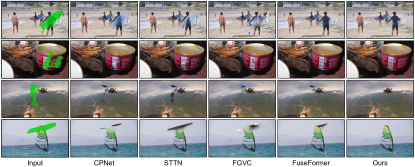
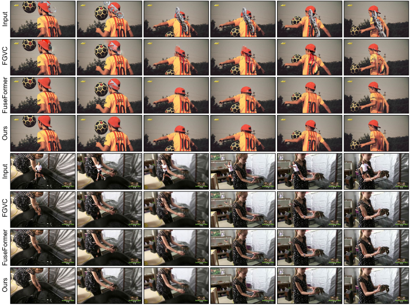
In Figure 5 and Figure 6, we qualitatively compare our method to state-of-the-art two-stage methods. As a VOS model, TBD (Cho et al. 2022b) is adopted for all VI models because it quantitatively outperforms other methods in Table 1. From Figure 5, we can conclude that optical flow-based methods, such as FGVC (Gao et al. 2020), are inadequate for OSVI. This is because un-erased objects may be copied and pasted to fill the object regions, and make the flow-based method produce the artifacts or some afterimages. Our method shows the clearest and most accurate object removal quality. Qualitative results are also compared in video form in Figure 6.
4.4 Ablation Study
In Table 2, we conduct an ablation study on various components of our method. Each different version is quantitatively compared on two synthesized datasets, DAYT and BLDA.
Mask loss. We conduct a study on the use of mask loss to figure out how mask supervision affects object removal quality. Removing mask loss leads to a drastic performance degradation as small errors in object regions lead to critical errors in the entire system. This demonstrates the need for mask supervision via mask loss is an essential component.
Mask guidance. To filter out object cues extracted from the feature encoder, we apply the mask guidance matrix in MMHA. The quantitative results demonstrate the effectiveness of this filtering process. Compared to the model version without filtering, the model version with filtering shows better performance on all metrics.
Multi-head attention. As TTB focuses on filling the object regions missing the object cues, we utilize STB to focus on filling the object regions that cannot be filled in TTB. Therefore, we apply the MMHA method only to TTB and not to STB. To prove its functionality, we evaluate the model version designed with MMHA instead of SMHA. It turns out that the employed masked attention was ineffective, in which it could not fill the object regions. Thus, the collaborative employment of masked attention for temporal information and naive attention for spatial information is required for OSVI.
End-to-end training. To demonstrate the effectiveness of end-to-end network training, we compare the models with and without the end-to-end training protocol. For the model without end-to-end training, the video completion module takes ground truth masks and extracted features without gradients to be separately trained from the mask prediction module. As observed from the table, end-to-end network training enables the network to be more effective. Meaningful improvements are observable for all metrics.
Encoder sharing. We also conduct an experiment to see the difference between models with single and multiple encoders. It is interesting to observe that using a single encoder shows much better performance than using separate encoders. This demonstrates that mask prediction and video completion share common complementary properties. Moreover, jointly learning them ensures a more appropriate network for OSVI.
5 Conclusion
Inspired by inefficiency of conventional VI methods for real-world applications, we deal with the task of OSVI only requiring a single-frame manual annotation. To better deal with this without merely sequentially connecting existing VOS and VI algorithms, we propose an end-to-end learnable baseline model. By a significant margin, our method outperforms all existing two-stage methods both quantitatively and qualitatively on two synthesized datasets. We believe our research makes a step towards efficient and applicable VI.
References
- Ba, Kiros, and Hinton (2016) Ba, J. L.; Kiros, J. R.; and Hinton, G. E. 2016. Layer normalization. arXiv preprint arXiv:1607.06450.
- Bešić and Valada (2020) Bešić, B.; and Valada, A. 2020. Dynamic Object Removal and Spatio-Temporal RGB-D Inpainting via Geometry-Aware Adversarial Learning. arXiv preprint arXiv:2008.05058.
- Caelles et al. (2017) Caelles, S.; Maninis, K.-K.; Pont-Tuset, J.; Leal-Taixé, L.; Cremers, D.; and Van Gool, L. 2017. One-shot video object segmentation. In Proceedings of the IEEE conference on computer vision and pattern recognition, 221–230.
- Chang, Yu Liu, and Hsu (2019) Chang, Y.-L.; Yu Liu, Z.; and Hsu, W. 2019. Vornet: Spatio-temporally consistent video inpainting for object removal. In Proceedings of the IEEE/CVF Conference on Computer Vision and Pattern Recognition Workshops, 0–0.
- Cheng and Schwing (2022) Cheng, H. K.; and Schwing, A. G. 2022. XMem: Long-Term Video Object Segmentation with an Atkinson-Shiffrin Memory Model. arXiv preprint arXiv:2207.07115.
- Cheng, Tai, and Tang (2021) Cheng, H. K.; Tai, Y.-W.; and Tang, C.-K. 2021. Modular Interactive Video Object Segmentation: Interaction-to-Mask, Propagation and Difference-Aware Fusion. In CVPR.
- Cho et al. (2022a) Cho, S.; Lee, H.; Kim, M.; Jang, S.; and Lee, S. 2022a. Pixel-Level Bijective Matching for Video Object Segmentation. In Proceedings of the IEEE/CVF Winter Conference on Applications of Computer Vision, 129–138.
- Cho et al. (2022b) Cho, S.; Lee, H.; Lee, M.; Park, C.; Jang, S.; Kim, M.; and Lee, S. 2022b. Tackling Background Distraction in Video Object Segmentation. arXiv preprint arXiv:2207.06953.
- Gao et al. (2020) Gao, C.; Saraf, A.; Huang, J.-B.; and Kopf, J. 2020. Flow-edge guided video completion. In European Conference on Computer Vision, 713–729. Springer.
- Hu, Huang, and Schwing (2018) Hu, Y.-T.; Huang, J.-B.; and Schwing, A. G. 2018. Videomatch: Matching based video object segmentation. In Proceedings of the European Conference on Computer Vision (ECCV), 54–70.
- Huang et al. (2016) Huang, J.-B.; Kang, S. B.; Ahuja, N.; and Kopf, J. 2016. Temporally coherent completion of dynamic video. ACM Transactions on Graphics (TOG), 35(6): 1–11.
- Kim et al. (2019) Kim, D.; Woo, S.; Lee, J.-Y.; and Kweon, I. S. 2019. Deep video inpainting. In Proceedings of the IEEE/CVF Conference on Computer Vision and Pattern Recognition, 5792–5801.
- Kingma and Ba (2014) Kingma, D. P.; and Ba, J. 2014. Adam: A method for stochastic optimization. arXiv preprint arXiv:1412.6980.
- Lee et al. (2019) Lee, S.; Oh, S. W.; Won, D.; and Kim, S. J. 2019. Copy-and-paste networks for deep video inpainting. In Proceedings of the IEEE/CVF International Conference on Computer Vision, 4413–4421.
- Li et al. (2020) Li, A.; Zhao, S.; Ma, X.; Gong, M.; Qi, J.; Zhang, R.; Tao, D.; and Kotagiri, R. 2020. Short-Term and Long-Term Context Aggregation Network for Video Inpainting. In European Conference on Computer Vision, 728–743. Springer.
- Li et al. (2022) Li, Z.; Lu, C.-Z.; Qin, J.; Guo, C.-L.; and Cheng, M.-M. 2022. Towards an end-to-end framework for flow-guided video inpainting. In Proceedings of the IEEE/CVF Conference on Computer Vision and Pattern Recognition, 17562–17571.
- Liang et al. (2020) Liang, Y.; Li, X.; Jafari, N.; and Chen, J. 2020. Video object segmentation with adaptive feature bank and uncertain-region refinement. Advances in Neural Information Processing Systems, 33: 3430–3441.
- Lin et al. (2014) Lin, T.-Y.; Maire, M.; Belongie, S.; Hays, J.; Perona, P.; Ramanan, D.; Dollár, P.; and Zitnick, C. L. 2014. Microsoft coco: Common objects in context. In European conference on computer vision, 740–755. Springer.
- Liu et al. (2021) Liu, R.; Deng, H.; Huang, Y.; Shi, X.; Lu, L.; Sun, W.; Wang, X.; Dai, J.; and Li, H. 2021. Fuseformer: Fusing fine-grained information in transformers for video inpainting. In Proceedings of the IEEE/CVF International Conference on Computer Vision, 14040–14049.
- Maninis et al. (2018) Maninis, K.-K.; Caelles, S.; Chen, Y.; Pont-Tuset, J.; Leal-Taixé, L.; Cremers, D.; and Van Gool, L. 2018. Video object segmentation without temporal information. IEEE transactions on pattern analysis and machine intelligence, 41(6): 1515–1530.
- Oh et al. (2019a) Oh, S. W.; Lee, J.-Y.; Xu, N.; and Kim, S. J. 2019a. Video object segmentation using space-time memory networks. In Proceedings of the IEEE International Conference on Computer Vision, 9226–9235.
- Oh et al. (2019b) Oh, S. W.; Lee, S.; Lee, J.-Y.; and Kim, S. J. 2019b. Onion-peel networks for deep video completion. In Proceedings of the IEEE/CVF International Conference on Computer Vision, 4403–4412.
- Perazzi et al. (2016) Perazzi, F.; Pont-Tuset, J.; McWilliams, B.; Van Gool, L.; Gross, M.; and Sorkine-Hornung, A. 2016. A Benchmark Dataset and Evaluation Methodology for Video Object Segmentation. In Computer Vision and Pattern Recognition.
- Pont-Tuset et al. (2017) Pont-Tuset, J.; Perazzi, F.; Caelles, S.; Arbeláez, P.; Sorkine-Hornung, A.; and Van Gool, L. 2017. The 2017 DAVIS Challenge on Video Object Segmentation. arXiv:1704.00675.
- Robinson et al. (2020) Robinson, A.; Lawin, F. J.; Danelljan, M.; Khan, F. S.; and Felsberg, M. 2020. Learning Fast and Robust Target Models for Video Object Segmentation. In IEEE/CVF Conference on Computer Vision and Pattern Recognition (CVPR).
- Shetty, Fritz, and Schiele (2018) Shetty, R.; Fritz, M.; and Schiele, B. 2018. Adversarial scene editing: Automatic object removal from weak supervision. arXiv preprint arXiv:1806.01911.
- Vaswani et al. (2017) Vaswani, A.; Shazeer, N.; Parmar, N.; Uszkoreit, J.; Jones, L.; Gomez, A. N.; Kaiser, Ł.; and Polosukhin, I. 2017. Attention is all you need. Advances in neural information processing systems, 30.
- Voigtlaender et al. (2019) Voigtlaender, P.; Chai, Y.; Schroff, F.; Adam, H.; Leibe, B.; and Chen, L.-C. 2019. Feelvos: Fast end-to-end embedding learning for video object segmentation. In Proceedings of the IEEE Conference on Computer Vision and Pattern Recognition, 9481–9490.
- Voigtlaender and Leibe (2017) Voigtlaender, P.; and Leibe, B. 2017. Online adaptation of convolutional neural networks for the 2017 davis challenge on video object segmentation. In The 2017 DAVIS Challenge on Video Object Segmentation-CVPR Workshops, volume 5.
- Wexler, Shechtman, and Irani (2004) Wexler, Y.; Shechtman, E.; and Irani, M. 2004. Space-time video completion. In Proceedings of the 2004 IEEE Computer Society Conference on Computer Vision and Pattern Recognition, 2004. CVPR 2004., volume 1, I–I. IEEE.
- Woo et al. (2018) Woo, S.; Park, J.; Lee, J.-Y.; and Kweon, I. S. 2018. Cbam: Convolutional block attention module. In Proceedings of the European conference on computer vision (ECCV), 3–19.
- Xu et al. (2018) Xu, N.; Yang, L.; Fan, Y.; Yue, D.; Liang, Y.; Yang, J.; and Huang, T. 2018. Youtube-vos: A large-scale video object segmentation benchmark. arXiv preprint arXiv:1809.03327.
- Xu et al. (2019) Xu, R.; Li, X.; Zhou, B.; and Loy, C. C. 2019. Deep flow-guided video inpainting. In Proceedings of the IEEE/CVF Conference on Computer Vision and Pattern Recognition, 3723–3732.
- Yang, Wei, and Yang (2020) Yang, Z.; Wei, Y.; and Yang, Y. 2020. Collaborative video object segmentation by foreground-background integration. arXiv preprint arXiv:2003.08333.
- Zeng, Fu, and Chao (2020) Zeng, Y.; Fu, J.; and Chao, H. 2020. Learning Joint Spatial-Temporal Transformations for Video Inpainting. In European Conference on Computer Vision, 528–543. Springer.
- Zhang et al. (2020) Zhang, R.; Li, W.; Wang, P.; Guan, C.; Fang, J.; Song, Y.; Yu, J.; Chen, B.; Xu, W.; and Yang, R. 2020. Autoremover: automatic object removal for autonomous driving videos. In Proceedings of the AAAI Conference on Artificial Intelligence, volume 34, 12853–12861.
- Zou et al. (2021) Zou, X.; Yang, L.; Liu, D.; and Lee, Y. J. 2021. Progressive temporal feature alignment network for video inpainting. In Proceedings of the IEEE/CVF Conference on Computer Vision and Pattern Recognition, 16448–16457.