Generalization of the Kuramoto model to the Winfree model by a symmetry breaking coupling

Abstract

We construct a nontrivial generalization of the paradigmatic Kuramoto model by using an additional coupling term that explicitly breaks its rotational symmetry resulting in a variant of the Winfree Model. Consequently, we observe the characteristic features of the phase diagrams of both the Kuramoto model and the Winfree model depending on the degree of the symmetry breaking coupling strength for unimodal frequency distribution. The phase diagrams of both the Kuramoto and the Winfree models resemble each other for symmetric bimodal frequency distribution for a range of the symmetry breaking coupling strength except for region shift and difference in the degree of spread of the macroscopic dynamical states and bistable regions. The dynamical transitions in the bistable states are characterized by an abrupt (first-order) transition in both the forward and reverse traces. For asymmetric bimodal frequency distribution, the onset of bistable regions depends on the degree of the asymmetry. Large degree of the symmetry breaking coupling strength promotes the synchronized stationary state, while a large degree of heterogeneity, proportional to the separation between the two central frequencies, facilitates the spread of the incoherent and standing wave states in the phase diagram for a low strength of the symmetry breaking coupling. We deduce the low-dimensional equations of motion for the complex order parameters using the Ott-Antonsen ansatz for both unimodal and bimodal frequency distributions. We also deduce the Hopf, pitchfork, and saddle-node bifurcation curves from the evolution equations for the complex order parameters mediating the dynamical transitions. Simulation results of the original discrete set of equations of the generalized Kuramoto model agree well with the analytical bifurcation curves.

1 Introduction

Symmetry (translational or rotational) prevailing in the coupled dynamical networks due to the coupling geometry manifests in a wide variety of natural systems and in their intriguing macroscopic dynamical states tstp2017 . Nevertheless, symmetry breaking couplings are shown to be a source of a plethora of collective dynamical behavior that are inherent to it and are mostly inaccessible with the symmetry preserving couplings. In particular, networks of the paradigmatic Stuart-Landau oscillators with symmetry breaking coupling have been employed to unravel several collective dynamical states that mimic a variety of collective patterns observed in nature and technology. For instance, symmetry breaking coupling facilitates the transition from the homogeneous to an inhomogeneous steady states akev2013 , symmetry breaking interaction has been identified as an essential feature for the genesis of partially coherent inhomogeneous spatial patterns, namely chimera death state zamk2014 ; tb2015 ; kpvkc2015 . Multicluster oscillation death states have been observed in nonlocally coupled Stuart-Landau oscillators with symmetry breaking coupling ismk2015 . Further, the interplay of the nonisochronicity parameter and the symmetry breaking coupling is found to facilitate the onset of different variants of chimera death state such as multichimera death state and periodic chimera death states in nonlocally coupled Stuart-Landau oscillators kpvkc2016 . The effect of the symmetry breaking coupling has also been investigated on the phenomenon of reviving oscillations wei2017 . Recently, the effect of the symmetry breaking mean-field coupling on the phenomenon of the aging transition has also been investigatedConjugate couplings, a symmetry breaking coupling, have also been widely employed in the literature rkrr2007 ; amit2012 ; wei2022 . Note that the pointed out reports are only a tip of an ice-berg and not an exhaustive list of studies that employed symmetry breaking coupling using the network of the Stuart-Landau oscillators.

Despite the substantial investigations on the effect of the symmetry breaking coupling in networks of Stuart-Landau oscillators, there is a lacunae in understanding the nontrivial role of the symmetry breaking coupling in the phase only models, which indeed allows for exact analytical treatment of the macroscopic dynamical states in most cases. In particular, phase models such as Winfree and Kuramoto models, and their variants have been extensively employed in the literature to investigate the emergence of various intriguing collective dynamical states. Interaction among the phase oscillators in the Winfree model is modeled by a phase-dependent pulse function and a sensitive function. The former characterizes the mean-field, while the latter characterizes the response of the individual oscillators to the mean-field w:1 ; w:2 . Winfree model is one of its kind representing a class of pulse-coupled biological oscillators such as flashing of fire files In2 , applauding audience In7 and many more. Interaction among the phase oscillators in the Kuramoto model is modeled by the sine of difference between the phases of the oscillator and has been widely employed to investigate the emergence of spontaneous synchronization in a wide variety of biological, chemical, mechanical and physical, systems Kuramoto:1984 ; Acebron:2005 ; In1 . Examples include cardiac pacemaker In3 , Josephson junction arrays In6 , and power-grids In8 .

A recent study has generalized the Kuramoto model by including an additional interaction term that breaks the rotational symmetry of the dynamics explicitly and unveiled a rich phase diagram with stationary and standing wave phases due to the symmetry breaking interaction In10 . Specifically, the authors have considered unimodal frequency distributions and revealed the emergence of a stationary state, characterized by time independent amplitude and phase of the complex Kuramoto order parameter, facilitated by the symmetry breaking interaction, which is otherwise absent in the original Kuramoto model that allows for the rotational symmetry of the dynamics. Interesting, in this work, we elucidate that the Kuramoto model can be translated into the Winfree model by the introduction of the additional symmetry breaking coupling and consequently, one can obtain the phase diagrams of both these models simply by tuning the symmetry breaking parameter $q$, thereby bridging the dynamics of both the models. Note that the macroscopic dynamical states of the pulse coupled biological oscillators with different sensitive functions, characterizing the phase-response-curves of biological oscillators, are peculiar to the Winfree model and its generalizations, which are far from reach for the Kuramoto model and its variants. In particular, we consider both the unimodal and bimodal frequency distributions to explore the phase diagrams for various values of the symmetry breaking parameter $q$. On the one hand, we observe the typical phase diagram of the Kuramoto model characterized only by incoherent and standing wave states in the absence of the symmetry breaking interaction for the unimodal frequency distribution. On the other hand, we observe the phase diagram with incoherent state, standing wave pattern along with the synchronized stationary state and bistabilities among them, a typical nature of the Winfree model, for $q=1$. For an intermediate and increasing value of $q\in(0,1)$, one can find the onset of the stationary state and eventually the emergence of bistability among these states in the phase diagram, and enlargement of the bistable regions resulting in the phase diagram of the Winfree model.

All three states are also observed in both Kuramoto and Winfree models for symmetric bimodal frequency distributions along with the region of bistability. The degree of the spread of the different macroscopic dynamical states depends on the strength of the symmetry breaking parameter $q$. Interestingly, for asymmetric bimodal frequency distributions, increase in the degree of asymmetry of the frequency distributions favors the onset of bistable regions even for a rather low values of $q$, which otherwise cannot be observed with the symmetric bimodal and unimodal frequency distributions. We arrive at the phase diagrams by numerical simulation of the original equations of motion. We deduce the reduced low-dimensional evolution equations of motion for the order parameter using the Ott-Antonsen ansatz for both unimodal and bimodal frequency distributions. We also deduce the Hopf, pitchfork and saddle-node bifurcation curves from the governing equations of motion for the order parameters, which mediates the dynamical transitions in the phase diagrams. Homoclinic bifurcation curve is obtained from the XPPAUT software.

The plan of the paper is as follows. In Sec. II, we generalize the Kuramoto model by introducing a symmetry breaking coupling and elucidate that the latter bridges the Kuramoto model and the Winfree model. We deduce the reduced low-dimensional evolution equations for the complex order parameters corresponding to the discrete set of generalized Kuramoto model using the Ott-Antonsen ansatz for both unimodal and bimodal frequency distributions in Sec. III. We also deduce Hopf, pitchfork and saddle-node bifurcation curves from the evolution equations for the complex order parameters in Sec. III, mediating the dynamical transitions among the incoherent, standing wave and synchronized stationary states. In Sec. IV, we discuss the observed dynamical states and their transitions in the various phase diagrams. Finally, in Sec. VI, we summarize the results.

2 Model

We consider a nontrivial generalization of the Kuramoto model by including an interaction term that explicitly breaks the rotational symmetry of the dynamics In10 . The phase $\theta_{i}$ is governed by the set of N ordinary differential equations (ODEs),

$$\dot{\theta_{i}} =\omega_{i}+\frac{\varepsilon}{N}\sum_{j=1}^{N}\big{[}\sin(\theta_{j}-\theta_{i})+q\sin(\theta_{j}+\theta_{i})\big{]},$$ (1)

for $i=1,\ldots,N$, where $N\gg 1$. Here $\theta_{i}(t)$ is the phase of the $i$th oscillator at time $t$, $\varepsilon\geq 0$ is the coupling strength, and $q$ is the strength of the symmetry breaking coupling. Note that Eq. (1) reduces to the Kuramoto model by setting $q=0$ and on identifying $\varepsilon$ with the parameter $K>0$. Equation (1) can also be viewed as a variant of the celebrated Winfree model w1 ; w2 ; w3 ; w4 when $q=1$. The Winfree model takes the form

$$\dot{\theta_{i}}=\omega_{i}+Q(\theta_{i})\sum_{j=1}^{N}P(\theta_{j}),$$ (2)

where $P(\theta_{j})$ is the phase dependent pulse function and the functional form of the response function $Q(\theta)$ characterizes the phase-response curves of certain biological oscillators. From Eq. (1), it easy to recognize that $Q(\theta)={-}2\sin(\theta)$ and $P(\theta)=\cos(\theta)$. It is also evident that the symmetry breaking parameter ‘q’ bridges the Kuramoto and the Winfree models. Equation (1) corresponds to the Kuramoto model when $q=0$ and it corresponds to a variant of the Winfree model when $q=1$, as in Eq. (2). We consider the frequencies of the phase-oscillators are distributed both by the unimodal Lorentzian distribution given as

$$g(\omega) =\frac{\gamma}{\pi((\omega-\omega_{0})^{2}+\gamma^{2})}\mathchar 24635\relax\;~{}~{}\gamma>0,$$ (3)

and bimodal Lorentzian distribution represented as

$$g(\omega) =\frac{1}{\pi}\left[\frac{\gamma_{1}}{((\omega-\omega_{0})^{2}+\gamma_{1}^{2})}+\frac{\gamma_{2}}{((\omega+\omega_{0})^{2}+\gamma_{2}^{2})}\right]\mathchar 24635\relax\;~{}~{}~{}~{}~{}~{}~{}~{}\gamma_{1},\gamma_{2}>0.$$ (4)

Here $\gamma$, $\gamma_{1}$ and $\gamma_{2}$ are the width parameter (half width at half maximum) of the Lorentzian and $\pm\omega_{0}$ are their central frequencies. Note that $\omega_{0}$ corresponds to the degree of detuning in the system, which is proportional to the separation between the two central frequencies. Note that the bimodal distribution $g(\omega_{0})$ is symmetric about zero when $\gamma_{1}=\gamma_{2}$. It is also to be noted that $g(\omega_{0})$ in Eq. (4) is bimodal if and only if the separation between their central frequencies are sufficiently greater than their widths. To be precise, it is required that $\omega_{0}>\gamma_{1,2}/\sqrt{3}$ for the distribution to be a bimodal, otherwise the classical results of the unimodal distribution holds good.

Heterogeneity in the frequency distribution plays a crucial role in the manifestation of a plethora of collective dynamics in a vast variety of natural systems. In particular, coexisting co-rotating and counter-rotating systems characterized by positive and negative frequencies, respectively, are wide spread in nature. For instance, counter-rotating spirals are observed in protoplasm of the Physarum plasmodium ref1 , counter-rotating vortices are inevitable in the atmosphere and ocean ref2 ; ref3 ; ref4 , in magnetohydrodynamics of plasma flow ref8 , Bose-Einstein condensates ref9 ; ref10 , and in other physical systems ref5 ; ref6 ; ref7 . Very recently, the counter-rotating frequency induced dynamical effects were also reported in the coupled Stuart-Landau oscillator with symmetry preserving as well as symmetry breaking couplings ref11 . The coexistence of co-rotating and counter-rotating oscillators was initially identified by Tabor ref12 , which is followed by a series of work employing co-rotating and counter-rotating oscillators. All these physical systems strongly suggest that counter-rotating time-evolving dynamical systems indeed exist in nature and play a pertinent role in the manifestation of their intriguing collective dynamics.

In the following, we will deduce the low-dimensional evolution equations for the complex macroscopic order parameters corresponding to both the unimodal and bimodal frequency distributions using the Ott-Antonsen (OA) ansatz Ott:2008 ; Ott:2009 . Subsequently, we also deduce the various bifurcation curves facilitating the dynamical transitions among the observed dynamical states in the phase diagrams.

3 Low-dimensional evolution equations for the macroscopic order parameters

We now provide an analysis of the dynamics (1), in the limit $N\to\infty$, by invoking the Ott-Antonsen ansatz. In this limit, the dynamics of the discrete set of equations (1) can be captured by the probability distribution function $f(\theta,\omega,t)$, defined such that $f(\theta,\omega,t){\rm d}\theta$ gives the probability of oscillators with phase in the range $[\theta,\theta+{\rm d}\theta]$ at time $t$. The distribution is $2\pi$-periodic in $\theta$ and obeys the normalization

$$\int_{0}^{2\pi}{\rm d}\theta~{}f(\theta,\omega,t)=g(\omega)~{}\forall~{}\omega.$$ (5)

Since the dynamics (1) conserves the number of oscillators with a given $\omega$, the time evolution of $f$ follows the continuity equation

$$\frac{\partial f}{\partial t}+\frac{\partial(fv)}{\partial\theta}=0,$$ (6)

where $v(\theta,\omega,t)$ is the angular velocity of the oscillators. From Eq. (1), we have,

$$v(\theta,\omega,t)=\omega+\frac{\varepsilon}{2i}[(ze^{-i\theta}-z^{\star}e^{i\theta})+q(ze^{i\theta}-z^{\star}e^{-i\theta})],$$ (7)

where $z^{\star}$ denotes the complex conjugate of the macroscopic order parameter defined as

$$z=\int_{-\infty}^{\infty}g(\omega)\int_{0}^{2\pi}f(\theta,\omega,t)e^{i\theta}d\theta d\omega.$$ (8)

Now, $f(\theta,\omega,t)$ can be expanded in terms of Fourier series of the form

$$f(\theta,\omega,t)=\frac{g(\omega)}{2\pi}\left[1+\sum_{n=1}^{\infty}\left(\alpha_{n}(\omega,t)e^{in\theta}+{\rm c.c.}\right)\right],$$ (9)

where, $\alpha_{n}(\omega,t)$ is the $n$th Fourier coefficient, while c.c. denotes complex conjugation of the preceding sum within the brackets. The normalization condition in (5) is satisfied by the presence of the prefactor of $g(\omega)$ in (9). The Ott-Antonsen ansatz consists in assuming Ott:2008 ; Ott:2009

$$\alpha_{n}(\omega,t)=\left[\alpha(\omega,t)\right]^{n}.$$ (10)

Now, it is straightforward to obtain

$$\frac{\partial\alpha}{\partial t}+i\omega\alpha+\frac{\varepsilon_{1}}{2}\left[(z\alpha^{2}-z^{\star})+q(z-z^{\star}\alpha^{2})\right],$$ (11)

where,

$$z^{\star}=\int_{-\infty}^{\infty}\alpha(t,\omega)g(\omega)d\omega.$$ (12)

3.1 Unimodal Distribution

Substituting the partial fraction expansion of the unimodal frequency distribution $g(\omega)$ (3) in Eq. (12) and evaluating the integral using an appropriate contour integral, one can obtain the order parameter as

$$z(t)=a^{\star}(\omega_{0}-i\gamma,t).$$ (13)

From (11) and (13), one can obtain the evolution equation for the complex order parameter as The above evolution equation for the complex order parameter $z(t)=r(t)e^{i\psi(t)}$ can be expressed in terms of the evolution equations in $r$ and $\psi$ as

$$\frac{{\rm d}r}{{\rm d}t} =-\gamma r-\frac{r\varepsilon}{2}(r^{2}-1)(1-q\cos(2\psi)),$$ (15a)

$$\frac{{\rm d}\psi}{{\rm d}t} =\omega_{0}+\frac{{\varepsilon}q}{2}(r^{2}+1)\sin(2\psi)).$$ (15b)

The above equations govern the reduced low-dimensional order parameter dynamics, which actually corresponds to the dynamics of the original discrete set of equations (1) in the limit $N\to\infty$ for the unimodal Lorentzian distribution function $g(\omega)$ (3). Now, we discuss the various asymptotic macroscopic dynamical states admitted by Eq. (15).

3.1.1 Incoherent (IC) state:

The incoherent (IC) state is characterized by time independent $z$ satisfying $z=z^{\star}=0$ (thus representing a stationary state of the dynamics (15)); correspondingly, one has $r=0$. The linear stability of such a state is determined by linearizing Eq. (LABEL:eq:z-dynamics) around $z=0$. By representing $z=u$ with u≪$1,weobtain\begin{equation}\frac{\partial u}{\partial t}+(\gamma-i\omega_{0})u-\frac{\varepsilon}{2}\big{[}(u)-q(u^{\star})\big{]}=0.\end{equation}Decomposing$u=u_x + i u_y

$$~{}~{}M\equiv\begin{bmatrix}-\gamma+\frac{\varepsilon}{2}\big{[}1-q\big{]}&-\omega_{0}\\ \\ ~{}\omega_{0}&-\gamma+\frac{\varepsilon}{2}\big{[}1+q\big{]}\\ \end{bmatrix}.$$

Thematrix

M$hasthecharacteristiceigenvalues\begin{equation}\lambda_{1,2}=\frac{-2\gamma+\varepsilon\pm\sqrt{\Delta}}{2},\end{equation}with$Δ=(ε^2q^2-4ω_0^2)$.Notethatwehave$λ_1 > λ_2$.Thestabilitythresholdfortheincoherentstateisthenobtainedbyanalysing$λ_1$asafunctionof$ε$and$q$,andseekingtheparticularvalueof$ε$atwhich$λ_1$vanishesforagiven$q$.Thestabilitythresholdcanbeobtainedas\begin{aligned} &\varepsilon_{HB}=2\gamma,~{}~{}~{}~{}~{}~{}~{}~{}~{}~{}~{}~{}~{}~{}~{}~{}~{}~{}~{}~{}~{}~{}~{}~{}~{}~{}~{}~{}\;\;\;\mbox{for}\;\;\Delta\leq 0,\\ &\varepsilon_{PF}=2\sqrt{\frac{\gamma^{2}+\omega_{0}^{2}}{1+q^{2}}}~{}~{}~{}~{}~{}~{}~{}~{}~{}~{}~{}~{}~{}~{}~{}~{}~{}~{}~{}~{}\mbox{for}\;\;\Delta>0.\end{aligned}$

3.1.2 Synchronized stationary state (SSS):

Now, we explore the possibility of existence of the synchronized stationary state. Requiring that $r$ and $\psi$ have time-independent non-zero values in this case and hence equating the left hand side of equations (15) to zero, we obtain the two coupled equations for the synchronized stationary state as

$$\frac{\varepsilon q}{2}\cos(2\psi) =\frac{\gamma}{(r^{2}-1)}+\frac{\varepsilon}{2},$$ (19a)

$$\frac{\varepsilon q}{2}\sin(2\psi) =-\frac{\omega_{0}}{(r^{2}+1)}.$$ (19b)

With some algebra, one can obtained the following expressions for the stationary $r$ and $\psi$:

$$\frac{\varepsilon^{2}q^{2}}{4} =\bigg{(}\frac{\gamma}{(r^{2}-1)}+\frac{\varepsilon}{2}\bigg{)}^{2}+\bigg{(}\frac{\omega_{0}}{(r^{2}+1)}\bigg{)}^{2},$$ (20a)

$$\tan(2\psi) =\frac{(1-r^{2})(\omega_{0})}{(r^{2}+1)(\gamma+\frac{\varepsilon}{2}(r^{2}-1))}.$$ (20b)

$r$ and $\psi$ can be calculated for a fixed set of parameters by numerically solving the above set of equations, which is then substituted back into the evolution equations for the low-dimensional order parameters to deduce the characteristic equation. The eigenvalues of the characteristic equation is then used to determine the saddle-node bifurcation curve in the suitable two parameter phase.

3.2 Bimodal Distribution

Now, we will deduce the low-dimensional evolution equations corresponding to the macroscopic order parameters for the original discrete set of equations (1) in the limit $N\to\infty$ for the asymmetric bimodal Lorentzian distribution function $g(\omega)$ (4). Expanding the latter using partial fractions and evaluating the integral in Eq. (12) using appropriate contour integral, one can obtained the complex order parameter as

$$z(t)=\frac{1}{2}[z_{1}(t)+z_{2}(t)],$$ (21)

where

$$z_{1,2}(t)=\alpha^{\star}(\pm\omega_{0}-i\gamma_{1,2},t).$$ (22)

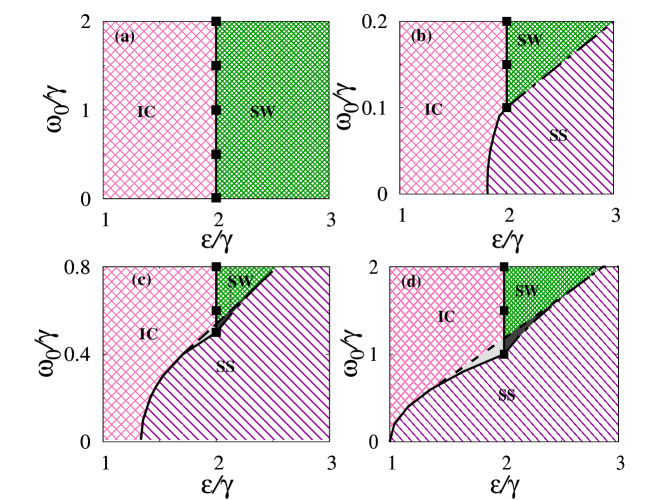
Figure 1: Phase diagrams in the $(\omega_{0}/\gamma,\varepsilon/\gamma)$ parameter space for the generalized Kuramoto model (1) with unimodal frequency distribution for different values of the symmetry breaking parameter $q$. (a) $q=0.0$, (b) $q=0.1$, (c) $q=0.5$, and (d) $q=1.0$. The line connected by filled squares is the Hopf bifurcation curve $\varepsilon_{HB}$ (Eq. (3.1.1)), solid line corresponds to the pitchfork bifurcation curve $\varepsilon_{PF}$ (Eq. (3.1.1)) dashed line corresponds to the saddle-node bifurcation curve (Eq. (20)), and the dashed dotted line correspond to the homoclinic bifurcation curve obtained using the software XPPAUT. Bistability between the standing wave (SW) state and the synchronized stationary (SS) state is represented by dark shaded region enclosed by the saddle-node bifurcation curve and the homoclinic bifurcation curve. Bistability between the incoherent (IC) and the SS state is represented by light grey shaded region enclosed by the saddle-node bifurcation curve and the pitchfork bifurcation curve.

Figure 2: Time averaged order parameter $R$ and the Shinomoto-Kuramoto order parameter $\xi$ for the generalized Kuramoto model (1) with unimodal frequency distribution as a function of $\varepsilon/\gamma$ for $\omega_{0}/\gamma=1$. (a) and (d) $q=0.0$ , (b) and (e) $q=0.5$, and (c) and (f) $q=1.0$. The forward trace is indicated by the line connected by open circles, while the reverse trace is indicated by the line connected by closed circles. The states indicated by IC, SW and SS correspond to the incoherent, standing wave, and synchronized stationary states, respectively. The bifurcation curves $\varepsilon_{HB},\varepsilon_{Hc},\varepsilon_{PF}$ and $\varepsilon_{SN}$ correspond to the Hopf, homoclinic, pitchfork and saddle-node bifurcation curves, respectively.

Substitution it into Eq. (11) yields two coupled complex ordinary differential equations describing the evolution of two suborder parameters as

$$\dot{z}_{1}= -(\gamma_{1}+i\omega_{0})z_{1}+\frac{\varepsilon}{4}[(z_{1}+z_{2}-(z_{1}^{\star}+z_{2}^{\star})z_{1}^{2})$$

$$+q((z_{1}+z_{2})z_{1}^{2}-(z_{1}^{\star}+z_{2}^{\star}))],$$ (23)

$$\dot{z}_{2}= -(\gamma_{2}-i\omega_{0})z_{2}+\frac{\varepsilon}{4}[(z_{1}+z_{2}-(z_{1}^{\star}+z_{2}^{\star})z_{2}^{2})$$

$$+q((z_{1}+z_{2})z_{2}^{2}-(z_{1}^{\star}+z_{2}^{\star}))].$$ (24)

The above evolution equations for the complex order parameters $z(t)_{1,2}=r(t)_{1,2}e^{i\psi(t)_{1,2}}$ can be expressed in terms of the evolution equations in $r_{1,2}$ and $\psi_{1,2}$, as

$$\frac{{\rm d}r_{1}}{{\rm d}t} =-\gamma_{1}r_{1}+\frac{\varepsilon}{4}\big{[}(1-r_{1}^{2})(r_{1}+r_{2}\cos(\psi_{2}-\psi_{1}))$$

$$+q((r_{1}^{2}-1)(r_{1}\cos(2\psi_{1})+r_{2}\cos(\psi_{2}+\psi_{1})))\big{]},~{}~{}~{}$$ (25a)

$$\frac{{\rm d}\psi_{1}}{{\rm d}t} =-\omega_{0}+\frac{{\varepsilon}}{4r_{1}}(r_{1}^{2}+1)\big{[}r_{2}\sin(\psi_{2}-\psi_{1})$$

$$+q(r_{1}\sin(2\psi_{1})+r_{2}\sin(\psi_{2}+\psi_{1}))\big{]}.$$ (25b)

and

$$\frac{{\rm d}r_{2}}{{\rm d}t} =-\gamma_{2}r_{2}+\frac{\varepsilon}{4}\big{[}(1-r_{2}^{2})(r_{1}\cos(\psi_{2}-\psi_{1})+r_{2})$$

$$+q((r_{2}^{2}-1)(r_{1}\cos(\psi_{2}+\psi_{1})+r_{2}\cos(2\psi_{2})))\big{]},~{}~{}~{}~{}$$ (26a)

$$\frac{d\psi_{2}}{dt} =\omega_{0}-\frac{{\varepsilon}}{4r_{2}}(r_{2}^{2}+1)\big{[}r_{1}\sin(\psi_{2}-\psi_{1})$$

$$-q(r_{1}\sin(\psi_{2}+\psi_{1})+r_{2}\sin(2\psi_{2}))\big{]}.$$ (26b)

The above equations constitute the evolution equations for reduced low-dimensional order parameters corresponding to the dynamics (1) in the limit $N\to\infty$ and for the case of the asymmetric bimodal Lorentzian distribution $g(\omega)$ (4). Now, we discuss the various asymptotic macroscopic dynamical states admitted by Eqs. (25) and (26).

3.2.1 Incoherent state

The incoherent state is defined by $r_{1}$=$r_{2}$=0. A linear stability analysis of the fixed point $(z_{1},z_{2})$ = (0, 0) results in the stability condition,

$$\omega_{0}^{2}=\frac{1}{4}(\varepsilon a_{1}-2a_{2}+\sqrt{\varepsilon^{2}q^{2}a_{1}-4\varepsilon a_{3}^{2}+4a_{3}^{2}a_{1}}),$$ (27)

where, $a_{1}=\gamma_{1}+\gamma_{2},a_{2}=\gamma_{1}^{2}+\gamma_{2}^{2}$ and $a_{3}=\gamma_{1}-\gamma_{2}$. This stability curve actually corresponds to the pitchfork bifurcation curve across which the fixed point $(z_{1},z_{2})$ = (0, 0) (incoherent state) loses its stability leading to the synchronized stationary state. Note that the incoherent state loses it stability through the Hopf bifurcation, which results in the stability condition

$$\omega_{0}^{2}= \frac{1}{4}(\varepsilon-2b_{1})^{4}(\varepsilon^{2}(q^{2}-1)-16b_{2}+4\varepsilon b_{1})^{2}\bigg{[}\varepsilon^{5}(q-1)b_{1}-\varepsilon^{4}(q^{2}-1)\big{(}(q^{2}-8)b_{3}$$

$$+2b_{2}(q^{2}-10)\big{)}-4\varepsilon^{3}(q^{2}-2)\big{(}3(\gamma_{1}^{3}+\gamma_{2}^{3})+13b_{2}b_{1}\big{)}+4\varepsilon^{2}(b_{1})^{2}\big{(}b_{3}(q^{2}-8)$$

$$+2b_{2}(3q^{2}-20)\big{)}+16\varepsilon b_{1}^{3}(b_{3}+10b_{2})-64b_{2}b_{1}^{4}\bigg{]},$$ (28)

where, $b_{1}=\gamma_{1}+\gamma_{2},b_{2}=\gamma_{1}\gamma_{2}$ and $b_{3}=\gamma_{1}^{2}+\gamma_{2}^{2}$. The above stability curve corresponds to the Hopf bifurcation curve. The boundary of stable incoherent state is therefore enclosed by both the pitchfork bifurcation and Hopf bifurcation curves.

3.2.2 Synchronized stationary state

Deducing the solution for the synchronized stationary state for the asymmetry bimodal distribution may not be possible as $r_{1}~{}\neq~{}r_{2}$ and $\psi_{1}~{}\neq~{}\psi_{2}$. However, for the symmetry bimodal distribution characterized by $r_{1}~{}=~{}r_{2}$ and $\psi_{1}~{}=~{}-\psi_{2}$, one can deduce the equations for $r$ and $\psi$ as in (20) and obtain the saddle-node bifurcation curves as pointed out in Sec. 3.1.2.

Figure 3: Phase diagrams in the $q-\varepsilon/\gamma$ parameter space for the generalized Kuramoto model (1) with unimodal frequency distribution for increasing degree of heterogeneity of the frequency distribution. (a) $\omega_{0}/\gamma_{2}=0.4$, (b) $\omega_{0}/\gamma_{2}=0.6$, (c) $\omega_{0}/\gamma_{2}=1.0$, and (a) $\omega_{0}/\gamma_{2}=1.2$. The bifurcation curves and dynamical states are similar to those in Fig. 1.

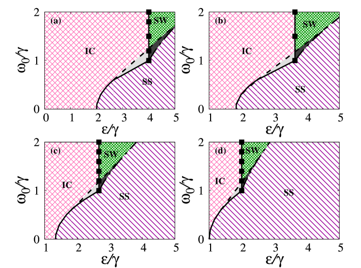
Figure 4: Phase diagrams in the $\omega_{0}/\gamma-\varepsilon/\gamma$ parameter space for the generalized Kuramoto model (1) with symmetric bimodal frequency distribution for increasing values of the strength of the symmetry breaking coupling. (a) $q=0.0$, (b) $q=0.5$, (c) $q=0.8$, and (d) $q=1.0$. The bifurcation curves and dynamical states are similar to those in Fig. 1.

Figure 5: Phase diagrams in the $\omega_{0}/\gamma_{2}-\varepsilon/\gamma_{2}$ parameter space for the generalized Kuramoto model (1) with asymmetric bimodal frequency distribution for increasing the strength of the symmetry breaking coupling and increasing the asymmetry between the bimodal frequency distributions. (a) and (b) $\gamma_{1}/\gamma_{2}=0.6$, and (c) and (d) $\gamma_{1}/\gamma_{2}=1.2$. (a) and (c) $q=0.1$ and (b) and (d) $q=1$. The bifurcation curves and dynamical states are similar to those in Fig. 1.

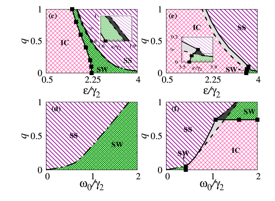
Figure 6: Phase diagrams in the $q-\varepsilon/\gamma_{2}$ parameter space (first row) for $\omega_{0}/\gamma_{2}=1$ and $q-\omega_{0}/\gamma_{2}$ (second row) for $\varepsilon/\gamma_{2}=2.5$ for the generalized Kuramoto model (1) with asymmetric bimodal frequency distribution. (a) and (c) $\gamma_{1}/\gamma_{2}=0.6$, and (b) and (d) $\gamma_{1}/\gamma_{2}=1.2$.

4 Numerical Results

In this section, we will proceed to unravel the macroscopic dynamical states admitted by the generalized Kuramoto model (1) with explicit symmetry breaking coupling by constructing appropriate two parameter phase diagrams and classifying the underlying dynamical states from a numerical analysis of the governing equations of the original discrete model. Specifically, we will unravel the rich phase diagrams of the generalized Kuramoto model, using both unimodal and bimodal frequency distributions, for distinct values of the symmetry breaking parameter $q$. The number of oscillators is fixed as N = $10^{4}$, and we use the standard 4th-order Runge-Kutta integration scheme with integration step size h = 0.01 to solve the generalized Kuramoto model (1). Note that one can break the two-parameter phase into several segments and multiple copies of the same code can be simulated simultaneously for different values of the parameters to generate the data, which can then be concatenated to get the complete phase diagrams with a reasonable workstation.

The initial state of the oscillators ($\theta_{i}$’s ) is distributed with uniform random values between -$\pi$ and +$\pi$. We use the time averaged order parameter $R$ defined as

$$R=\lim_{t\to\infty}\frac{1}{\tau}\int_{t}^{t+\tau}r(t)dt,$$ (29)

where $r(t)=|Z|=|N^{-1}\sum_{j=1}^{N}e^{i\theta_{j}}|$. Incoherent state is characterized by $R=r(t)=0$, while the synchronized stationary state is characterized by $R=r(t)=const.$ Standing wave is characterized by the oscillating nature of $r(t)$. In order to distinguish the synchronized stationary state and the standing wave state more clearly, we use the Shinomoto-Kuramoto order parameter gallego ; ssyk1986

$$\xi=\overline{|r(t)-R|},$$ (30)

where $\bar{z}$ denoted the long time average. Shinomoto-Kuramoto order parameter takes $\xi=0$ for the incoherent and synchronized stationary states, whereas it takes nonzero value for the standing wave state.

4.0.1 Phase diagrams for the unimodal distribution

We have depicted phase diagrams in the ($\omega_{0}/\gamma,\varepsilon/\gamma$) parameter space for different values of the symmetry breaking parameter $q$ in Fig. 1 in order to understand the effect of the explicit symmetry breaking interaction on the dynamics of Eq. (1) with unimodal frequency distribution. The phase diagram is demarcated into different dynamical regions using the value of the time averaged order parameter $R$ and the Shinomoto-Kuramoto order parameter $\xi$. Incoherent state (IC), synchronized stationary state (SS) and standing wave (SW), along with the bistable regions (dark and light gray shaded regions) are observed in the phase diagram. The parameter space indicated by light gray shaded region corresponds to the bistable regime between the incoherent and the synchronized stationary states, while that indicated by dark gray shaded region corresponds to the bistable regime between the standing wave and the synchronized stationary states,

Only the incoherent and standing wave states are observed in the phase diagram for $q=0$ (see  1(a)), a typical phase diagram of the Kuramoto model with unimodal frequency distribution. The line connected by the filled squares corresponds to the Hopf bifurcation curve, across which there is a transition from the incoherent state to the standing wave state. Note that a finite value of $q$ results in the loss of the rotational symmetry of the dynamics of the Kuramoto oscillators. Even a feeble value of $q$ manifests the synchronized stationary state in a rather large parameter space at the cost of the standing wave state (see Fig. 1(b) for q=0.1). There is a transition from the incoherent state to the standing wave state via the Hopf bifurcation curve $\varepsilon_{HB}$ (indicated by the line connected by filled squares) as a function of $\varepsilon/\gamma$ for $\omega_{0}/\gamma>0.1$. The standing wave state loses its stability via the homoclinic bifurcation (indicated by the dashed-dotted line) as a function of $\varepsilon/\gamma$ resulting in the synchronized stationary state. There is also a transition from the incoherent state to the synchronized stationary state for $\omega_{0}/\gamma\leq 0.1$ as a function of $\varepsilon/\gamma$ via the pitchfork bifurcation curve $\varepsilon_{PF}$ indicated by the solid line.

Further larger values of the symmetry breaking parameter results in the emergence of the bistability between the standing wave and the synchronized stationary states (indicated by dark shaded region) enclosed by the saddle-node bifurcation curve (indicated by dashed line) and the homoclinic bifurcation curve (see Fig. 1(c) for q=0.5). There is also a bistable region between the incoherent state and the synchronized stationary state (indicated by light grey shaded region) enclosed by the saddle-node bifurcation curve and the pitchfork bifurcation curve. For $q=1$, both the bistable regions enlarged in the phase diagram (see Fig. 1(d)), which is a typical phase diagram of the Winfree model with the unimodal frequency distribution. The phase diagrams for $q=0.5$ and $1.0$ have similar dynamics except for the regime shift and enhanced bistabilities in a larger parameter space. Thus, as the value of $q$ is increased from the null value to the unity, one can observe the transition from the phase diagram of the Kuramoto model to that of the Winfree model. Note that the Hopf, saddle-node and pitchfork bifurcation curves are the analytical bifurcation curves, Eqs. (3.1.1), (3.1.1) and (20) respectively, obtained from the low-dimensional evolution equations for the order parameters deduced in Sec. 3.1. Homoclinic bifurcation curve is obtained from the software XPPAUT xpp .

Time averaged order parameter $R$ and the Shinomoto-Kuramoto order parameter $\xi$ are depicted in Fig. 2 as a function of $\varepsilon/\gamma$ for different values of the symmetry breaking parameter $q$ and $\omega_{0}/\gamma$. The forward trace is indicated by the line connected by open circles, while the backward trace is indicated by the line connected by closed circles. There is a smooth (second order) transition from the incoherent to the standing wave states via the Hopf bifurcation $\varepsilon_{HB}$ at $\varepsilon/\gamma=2$ during both forward and reverse traces for $q=0.0$ and $\omega_{0}/\gamma=1$ as depicted in Figs. 2(a) and 2(d). In addition, to the smooth transition from the incoherent state to the standing wave state via the Hopf bifurcation $\varepsilon_{HB}$ at $\varepsilon/\gamma=2$, there is another smooth transition from the standing wave state to the synchronized stationary state via the homoclinic bifurcation $\varepsilon_{Hc}$ at $\varepsilon/\gamma=2.94$ in both the forward and reverse traces as shown in Fig. 2(b) for $q=0.5$ and $\omega_{0}/\gamma=1$. The transition from the standing wave state to the synchronized stationary state is also corroborated by the sharp fall of the Shinomoto-Kuramoto order parameter $\xi$ to the null value (see Fig. 2(e)). In contrast, there is an abrupt (first order) transition from the incoherent state to the synchronized stationary state at $\varepsilon/\gamma=2$ via the pitchfork bifurcation curve $\varepsilon_{PF}$ for $\omega_{0}/\gamma=1$ during the forward trace, whereas there is an abrupt transition from the synchronized stationary state to the incoherent state at $\varepsilon/\gamma=1.8$ via the saddle-node bifurcation $\varepsilon_{SN}$ during the reverse trace (see Fig. 2(c) for $q=1.0$) elucidating the presence of hysteresis and bistability between the incoherent state and the synchronized stationary state. The Shinomoto-Kuramoto order parameter $\xi$ takes the null value, in the entire range of $\varepsilon/\gamma$ in Fig. 2(f) for $q=1.0$, characterizing both the incoherent and the synchronized stationary states.

The observed dynamical states and their transitions are depicted in the $(q,\varepsilon/\gamma)$ parameter space for different $\omega_{0}/\gamma$ in Fig. 3. The bifurcations mediating the dynamical transitions are similar to those observed in Fig. 1. The phase diagram for $\omega_{0}/\gamma=0.4$ is shown in Fig. 3(a). There is a transition from the incoherent state to the standing wave state via the Hopf bifurcation curve for smaller values of the symmetry breaking parameter as a function of $\varepsilon/\gamma$. Larger values of the symmetry breaking parameter favor the synchronized stationary state in the entire range of $\varepsilon/\gamma$. However, in a narrow range of $q\in(0.36,0.46]$ (see Fig. 3(a)), there is a transition from the incoherent state to the standing wave state and then to the synchronized stationary state. There is also a transition from the incoherent state to the synchronized stationary state in the range of $q\in(0.46,0.6)$. Recall that $\omega_{0}$ quantifies the degree of detuning of the frequency distribution. Increase in the heterogeneity of the frequency distribution promotes bistable regions, incoherent and standing wave states, to a large region of the $(q,\varepsilon/\gamma)$ parameter space. For instance, the phase diagram for $\omega_{0}/\gamma=0.6$ is depicted in Fig. 3(b) elucidates the emergence of the bistable regions and enlarged regions of the incoherent and standing wave states as a function of $q$, a manifestation of increased heterogeneity. Further increase in the $\omega_{0}/\gamma$ enlarges the bistable regions, the incoherent and the standing wave states as depicted in Figs. 3(c) and  3(d) for $\omega_{0}/\gamma=1$ and $1.2$, respectively. These results are in agreement with the phase diagrams in Fig. 1 in the $(\omega_{0}/\gamma,\varepsilon/\gamma)$ parameter space for increasing values of the symmetry breaking parameter. Next, we will explore the effect of symmetric and asymmetric bimodal frequency distributions on the phase diagrams in the following.

4.0.2 Phase diagrams for bimodal distribution

In this section, we analyse the phase space dynamics of the generalized Kuramoto model (1) with symmetric bimodal frequency distribution (4) by setting $\gamma=\gamma_{1}=\gamma_{2}$ for increasing values of the strength of the symmetry breaking coupling. We have depicted the phase diagrams in the $(\omega_{0}/\gamma,\varepsilon/\gamma)$ parameter space for different values of the symmetry breaking parameter $q$ in Fig. 4. Note that the phase space dynamics of the Kuramoto model (see Fig.  4(a) for $q=0$) are similar to those of the Winfree model (see Fig.  4(d) for $q=1$) for the symmetric bimodal frequency distribution except for the regime shift. The dynamical states and the bifurcation curves are similar to those in Fig. 1. Increasing the strength of the symmetry breaking coupling favors the synchronized stationary state and the bistable states in a large region of the parameter space as evident from Fig.  4(b) and  4(c) for $q=0.5$ and $q=0.8$, respectively. Note that a large heterogeneity in the frequency distribution favor the incoherent and the standing wave states in a rather large region of the phase diagram for smaller $q$ and $\varepsilon$ (see Fig.  4(a) for $q=0$). Nevertheless, the synchronized stationary state predominates the phase diagram for larger strength of the symmetry breaking coupling and $\varepsilon$ despite the presence of a large heterogeneity in the frequency distribution (see Fig.  4(d) for $q=1$).

Next, we analyze the phase space dynamics of the generalized Kuramoto model (1) with asymmetric bimodal frequency distribution (4) by increasing the strength of the symmetry breaking coupling and the degree of asymmetry between the bimodal frequency distributions. We have depicted the phase diagrams in the $(\omega_{0}/\gamma_{2},\varepsilon/\gamma_{2})$ parameter space for different values of the symmetry breaking parameter $q$ in Fig. 5. Again, the dynamical states and the bifurcation curves are similar to those in Fig. 1. Phase diagram for $q=0.1$ and $\gamma_{1}/\gamma_{2}=0.6$ is depicted in Fig. 5(a). For most values of $\omega_{0}/\gamma_{2}$, there is a transition from the incoherent state to the synchronized stationary state via the standing wave state and there is no bistability for $\gamma_{1}<\gamma_{2}$. However, there is a transition from the incoherent state to the synchronized stationary state in a large range of $\omega_{0}/\gamma\in(0,1)$ and the emergence of bistable states for $\gamma_{1}>\gamma_{2}$ as depicted in Fig. 5(b) for $\gamma_{1}/\gamma_{2}=1.2$. It is evident that bistable states emerge even for low values of the symmetry breaking coupling when $\gamma_{1}>\gamma_{2}$. Note that bistable states emerge even for $\gamma_{1}<\gamma_{2}$ but for a large strength of the symmetry breaking coupling (see Fig. 5(c) for $q=1$ and $\gamma_{1}/\gamma_{2}=0.6$). The spread of the bistable states increases for $q=1$ and $\gamma_{1}/\gamma_{2}=1.2$ as illustrated in Fig. 5(d). Thus, larger $\gamma_{1}/\gamma_{2}$ and $q$ favor the emergence of the bistable states.

Phase diagrams in the $(q,\varepsilon/\gamma_{2})$ parameter space is depicted in Figs. 6(a) and  6(b) for $\gamma_{1}/\gamma_{2}=0.6$ and $1.2$, respectively, and for $\omega_{0}/\gamma_{2}=1$. The dynamical states and the bifurcation curves are similar to those in Fig. 1. There is a transition from the incoherent state to the synchronized stationary state via the standing wave state for small values of $q$ (see Fig.. 6(a)) similar to that in Fig. 5(a). However, for larger values of $q$ multistability between the standing wave and the synchronized stationary state emerges (dark shaded region in the inset) in addition to the above dynamical transition. For $\gamma_{1}>\gamma_{2}$, there a transition from the incoherent state to the standing wave state along with the bistability among them in a rather narrow range of $q\in(0,0.4)$ as a function of $\varepsilon/\gamma_{2}$ as shown in inset of Fig. 6(b). For $q>0.4$, there is a transition from the incoherent state to the synchronized stationary state with the onset of bistability (light grey shaded region) between them. Phase diagrams in the $(q,\omega_{0}/\gamma_{2})$ parameter space is depicted in Figs. 6(c) and  6(d) for $\gamma_{1}/\gamma_{2}=0.6$ and $1.2$, respectively, for $\varepsilon/\gamma_{2}=2.5$. There is a transition from the synchronized stationary state to the standing wave state as a function of $\omega_{0}/\gamma_{2}$ for $\gamma_{1}<\gamma_{2}$ (see Fig. 6(c)) via the homoclinic bifurcation curve. Both the bistable states emerge when $\gamma_{1}>\gamma_{2}$ as shown in Fig. 6(c) for $\gamma_{1}=1.2$.

5 Conclusions

We have considered a nontrivial generalization of the paradigmatic Kuramoto model by using an additional coupling term that explicitly breaks the rotational symmetry of the Kuramoto model. The strength of the symmetry breaking coupling is found to play a key role in the manifestation of the dynamical states and their transitions along with the onset of bistability among the observed dynamical states in the phase diagram. A typical phase diagram of the Kuramoto model is transformed into a typical phase diagram of the Winfree mode for the unit value of the strength of the symmetry breaking coupling thereby bridging the dynamics of both the Kuramoto and Winfree models. Large values of the strength of the symmetry breaking coupling favor the manifestation of bistable regions and synchronized stationary state in a large region of the phase diagram. The dynamical transitions in the bistable region are characterized by an abrupt (first-order) transition in both the forward and reverse traces. Phase diagrams of both the Kuramoto and Winfree models resemble each other for symmetric bimodal frequency distribution except for the regime shifts and the degree of the spread of the dynamical states and bistable regions. Nevertheless, for asymmetric bimodal frequency distribution one cannot observe the bistable states for low values of the strength of the symmetry breaking coupling when $\gamma_{1}<\gamma_{2}$. In contrast, bistable states emerge even for $\gamma_{1}<\gamma_{2}$ for a large strength of the symmetry breaking coupling. Larger $\gamma_{1}/\gamma_{2}$ and larger $q$ favors the emergence of the bistable states in the case of the asymmetric bimodal frequency distribution. A large $\omega_{0}$ and consequently a large degree of heterogeneity facilitates the spread of the incoherent and standing wave states in the phase diagram for a low strength of the symmetry breaking coupling. However, a large $q$ promotes the spread of the synchronized stationary state and bistable regions in the phase diagram despite the degree of heterogeneity in the frequency distribution. We have deduced the low-dimensional evolution equations for the complex order parameters using the Ott-Antonsen ansatz for both unimodal and bimodal frequency distributions. We have also deduced the Hopf, pitchfork, saddle-node bifurcation curves from the low-dimensional evolution equations for the complex order parameters. Homoclinic bifurcation curve is obtained from XPPAUT software. Simulation results, obtained from the original discrete set of equations agrees well with the analytical bifurcation curves. We sincerely believe that our results will shed more light and enhance our current understanding of the effects of symmetry breaking coupling in the phase models and bridges the dynamics of two distinctly different phase models, which are far from reach otherwise.

6 Acknowledgements

The work of V.K.C. is supported by the DST-CRG Project under Grant No. CRG/2020/004353 and DST, New Delhi for computational facilities under the DST-FIST program (SR/FST/PS- 1/2020/135)to the Department of Physics. M.M. thanks the Department of Science and Technology, Government of India, for provid- ing financial support through an INSPIRE Fellowship No. DST/INSPIRE Fellowship/2019/IF190871. S.G. acknowledges support from the Science and Engineering Research Board (SERB), India under SERB-TARE scheme Grant No. TAR/2018/000023 and SERB-MATRICS scheme Grant No. MTR/2019/000560. He also thanks ICTP – The Abdus Salam International Centre for Theoretical Physics, Trieste, Italy for support under its Regular Associateship scheme. DVS is supported by the DST-SERB-CRG Project under Grant No. CRG/2021/000816.

Data Availability Statement: No Data associated in the manuscript. The data sets on the current study are available from the corresponding author on reasonable request.

References

- (1) T. Stankovski, T. Pereira, Peter V. E. McClintock and A. Stefanovska, Coupling functions: Universal insights into dynamical interactionmechanisms, Rev. Mod. Phys. 89 045001 (2017).
- (2) A. Koseska, E. Volkov and J. Kurths, Transition from Amplitude to Oscillation Death Via Turing Bifurcation, Phys. Rev. Lett. 111, 024103 (2013).
- (3) A. Zakharova, M. Kapeller, and E. Schöll, Chimera Death: Symmetry Breaking in Dynamical Networks, Phys. Rev. Lett. 112, 154101 (2014).
- (4) T Banerjee, Mean-field-diffusion induced chimera death state, EuroPhys. . Lett. 110, 69993 (2015).
- (5) K. Premalatha, V. K. Chandrasekar, M. Senthilvelan, and M. Lakshmanan, Impact of symmetry breaking in networks of globally coupled oscillators, Phys. Rev. E 91, 052915 (2015).
- (6) I. Schneider, M. Kapeller, S Loss, A. Zakharova, B. Fiedler and E. Schöll, Stable and transient multicluster oscillation death in nonlocally coupled networks, Phys. Rev. E 92, 052915 (2015).
- (7) K. Premalatha, V. K. Chandrasekar, M. Senthilvelan, and M. Lakshmanan, Different kinds of chimera death states in nonlocally coupled oscillators, Phys. Rev. E 93, 052213 (2016).
- (8) Wei Zou, Meng Zhan, and J. Kurths, The impact of propagation and processing delays on amplitude and oscillation deaths in the presence of symmetry-breaking coupling, Chaos 27, 114303 (2017). Trade-off between filtering and symmetry breaking mean-field coupling in inducing macroscopic dynamical states, New J. Phys. 22 093024 (2020).
- (9) R. Karnatak, R. Ramaswamy, and A. Prasad, Amplitude death in the absence of time delays in identical coupled oscillators, Phys. Rev. E 76, 035201(R) (2007).
- (10) Amit Sharma amd Manish Dev Shrimali Amplitude death with mean-field diffusion, Phys. Rev. E 85, 057204 (2012).
- (11) Wei Zou, S. He , and C. Yao, Stability of amplitude death in conjugate-coupled nonlinear oscillator networks, Appl. Math. Lett. 131, 108052 (2022).
- (12) A. T. Winfree, Biological Rhythms and the Behaviour of Populations of Coupled Oscillators, J. Theor. Biol. 16, 15 (1967).
- (13) A. T. Winfree, The Geometry of Biological Time (Springer, New York, 1980).
- (14) J. Buck, Synchronous Rhythmic Flashing of Fireflies II, Quart. Rev. Biol. 63, 265-289 (1988).
- (15) Z. Néda, E. Ravasz, T. Vicsek, Y. Brechet, and A. L. Barabasi, Physics of the rhythmic applause, Phys. Rev. E 61, 6987 (2000).
- (16) Y. Kuramoto, Chemical Oscillations, Waves and Turbulence (Springer, Berlin, 1984).
- (17) J. A. Acebron, L. L. Bonilla, C. J. P. Vicente, F. Ritort and R. Spigler, The Kuramoto model: a simple paradigm for synchronization phenomena, Rev. Mod. Phys. 77, 137 (2005).
- (18) A. Pikovsky, M. Rosenblum, and J. Kurths, Synchronization: A Universal Concept in Nonlinear Science(Cambridge University Press, Cambridge, 2001).
- (19) C. S. Peskin, Mathematical Aspects of Heart Physiology (Courant Institute of Mathematical Sciences, New York, 1975).
- (20) S. P. Benz and C. J. Burroughs,Coherent emission from two-dimensional Josephson junction arrays, Appl. Phys. Lett. 58, 2162 (1991).
- (21) M. Rohden, A. Sorge, M. Timme, and D. Witthaut, Self Organized Synchronization in Decentralized Power Grids, Phys. Rev. Lett. 109, 064101 (2012).
- (22) V. K. Chandrasekar, M. Manoranjani, and Shamik Gupta Kuramoto model in the presence of additional interactions that break rotational symmetry, Phys. Rev. E 102, 012206 (2020).
- (23) R. Gallego, E. Montbrio, and D. Pazo, Synchronization scenarios in the Winfree model of coupled oscillators, Phys. Rev. E 96, 042208 (2017).
- (24) Joel T. Ariaratnam, and S. H. Strogatz, Phase diagram for the Winfree model of coupled nonlinear oscillators, Phys. Rev. Lett. 86, 19 (2001).
- (25) F. Giannuzzi, D. Marinazzo, G. Nardulli, M. Pellicoro, and S. Stramalia, Phase diagram of a generalized Winfree model, Phys. Rev. E 75, 051104 (2007).
- (26) D. Pazo, and E. Montbrio, Low-dimensional dynamics of populations of pulse-coupled oscillators, Phys. Rev. X 4, 011009 (2014).
- (27) S. Takagi, T. Ueda, Emergence and transitions of dynamic patterns of thickness oscillation of the plasmodium of the true slime mold Physarum polycephalum, Physica D 237, 420 (2008).
- (28) Y. Murakami, H. Fukuta, Stability of a pair of planar counter-rotating vortices in a rectangular box, Fluid Dyn. Res. 31, 1 (2002).
- (29) H. Fukuta, Y. Murakami, Vortex merging, oscillation, and quasiperiodic structure in a linear array of elongated vortices, Phys. Rev. E 57, 449 (1998).
- (30) P. Meunier, T. Leweke, Elliptic instability of a co-rotating vortex pair, J. Fluid. Mech. 533, 125 (2005).
- (31) G.N. Throumoulopoulos, H. Tasso, Magnetohydrodynamic counter-rotating vortices and synergetic stabilizing effects of magnetic field and plasma flow, Phys. Plasmas 17, 032508 (2010).
- (32) K.T. Kapale, J.P. Dowling, Vortex phase qubit: Generating arbitrary, counterrotating, coherent superpositions in Bose-Einstein condensates via optical angular momentum beams, Phys. Rev. Lett. 95, 173601 (2005).
- (33) S. Thanvanthri, K. T. Kapale, and J. P. Dowling, Arbitrary coherent superpositions of quantized vortices in Bose-Einstein condensates via orbital angular momentum of light, Phys. Rev. A 77, 053825 (2008).
- (34) K. Czolczynski, P. Perlikowski, A. Stefanski, T. Kapitaniak, Synchronization of pendula rotating in different directions, Commun. Nonlin. Sci. Num. Simul. 17, 3658 (2012).
- (35) M. Kapitaniak, K. Czolczynsk, P. Perlikowski, A. Stefanski, T. Kapitaniak, Synchronous states of slowly rotating pendula, Phys. Rep. 541, 1 (2014).
- (36) K. Czolczynski, P. Perlikowski, A. Stefanski, T. Kapitaniak, Synchronization of slowly rotating pendulums, Int. J. Bifurc. Chaos 22, 1250128 (2012).
- (37) K. Sathiyadevi, V. K. Chandrasekar, and M. Lakshmanan, Emerging chimera states under nonidentical counter-rotating oscillators, Phys. Rev. E 105, 034211 (2022).
- (38) M. Tabor, Chaos and Integrability in Nonlinear Dynamics: An Introduction (John Wiley and Sons, New York, 1988).
- (39) E. Ott and T. M. Antonsen, Low dimensional behavior of large systems of globally coupled oscillators, Chaos 18, 037113 (2008).
- (40) E. Ott and T. M. Antonsen, Long time evolution of phase oscillator systems, Chaos 19, 023117 (2009).
- (41) R. Gallego, E. Montbrio, and D. Pazo, Phys. Rev. E 96, 042208 (2017).
- (42) S. Shinomoto, and Y. Kuramoto, Prog. Theor. Phys. 75, 1105 (1986).
- (43) B. Ermentrout, Simulating, Analyzing, and Animating Dynamical Systems: A Guide to XPPAUT for Researchers and Students (Society for Industrial & Applied Math, Philadelphia, PA, 2002).