Design of an Adaptive Lightweight LiDAR to Decouple Robot-Camera Geometry

Abstract

A fundamental challenge in robot perception is the coupling of the sensor pose and robot pose. This has led to research in active vision where robot pose is changed to reorient the sensor to areas of interest for perception. Further, egomotion such as jitter, and external effects such as wind and others affect perception requiring additional effort in software such as image stabilization. This effect is particularly pronounced in micro-air vehicles and micro-robots who typically are lighter and subject to larger jitter but do not have the computational capability to perform stabilization in real-time. We present a novel microelectromechanical (MEMS) mirror LiDAR system to change the field of view of the LiDAR independent of the robot motion. Our design has the potential for use on small, low-power systems where the expensive components of the LiDAR can be placed external to the small robot. We show the utility of our approach in simulation and on prototype hardware mounted on a UAV. We believe that this LiDAR and its compact movable scanning design provide mechanisms to decouple robot and sensor geometry allowing us to simplify robot perception. We also demonstrate examples of motion compensation using IMU and external odometry feedback in hardware.

I Introduction

Modern autonomy is largely driven by vision and depth sensors for perception. Most such techniques make an implicit assumption that the relative pose of the sensor w.r.t. the robot is fixed and changes in sensor viewpoint require a change in the robot pose. This implies that fast-moving robots must deal with motion compensation (i.e. camera-robot stabilization) and that robots need to reorient themselves to observe the relevant parts of the scene. Correspondingly, stabilization [32, 12, 43, 35] and active vision [7, 4, 60, 36] are well-studied problems.

Let us consider the specific example of image stabilization. While successful, most such methods compensate through post-capture processing of sensor data. We contend that this is simply not feasible for the next generation of fast miniature robots such as robotic bees [51], crawling and walking robots [18], and other micro-air vehicles [31]. For example, flapping-wing robots such as the RoboBee exhibit a high frequency rocking motion (at about 120 Hz in one design) due to the piezo-electric actuation [17]. Environmental factors such as wind affects micro-robots to a greater extent than a larger robot. There might be aerodynamic instability due ornithopter-based shock absorption [53]. The egomotion of small robots (and onboard sensors) is quite extreme making any sensing challenging. While there have been software methods to correct for such effects for cameras [6] and LiDARs [34], this is often difficult to perform in real-time onboard due to the computational, energy and latency constraints on the robot mentioned above. Without proper motion compensation for miniature devices, we will not be able to unlock the full potential of what is one of the ten grand challenges in robotics [54].

I-A Key Idea: Compensation during Imaging

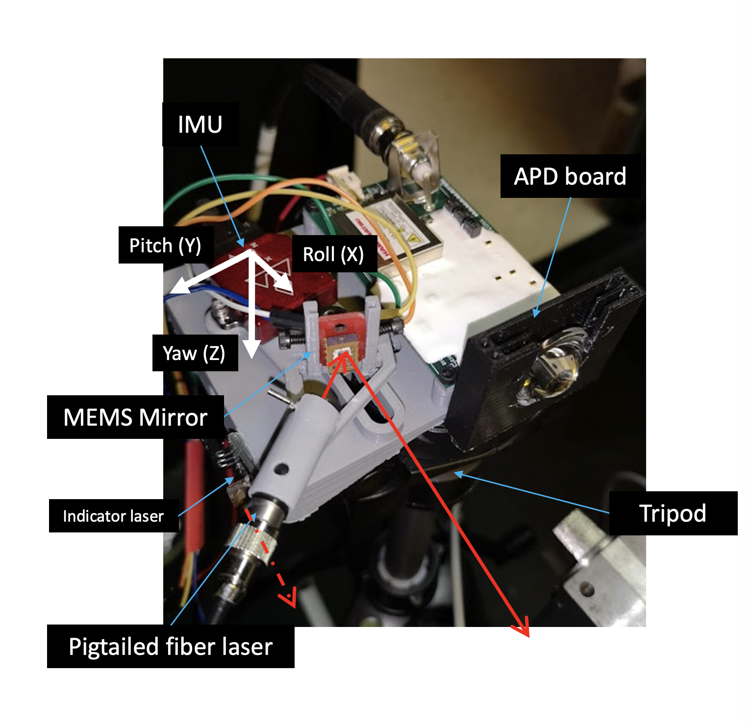
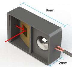
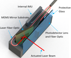
Figure 1: Our design is given above with the prototype motion-compensated LiDAR (up), and we also prepared a design for future work to integrate this onto smaller platforms.

Our idea is for motion correction to happen in sensor hardware during imaging such that measurements are already compensated without requiring onboard computing. This paper shows the motion compensation advantage of decoupling robot-camera geometry, and providing the ability to control the camera properties independent of the robot pose could bring about a new perspective to robot perception and simplify the autonomy pipeline. We demonstrate this through the design of a MEMS-driven LiDAR and perform compensation in two ways - (i) onboard IMU, and (ii) external feedback of robot pose at a high rate.

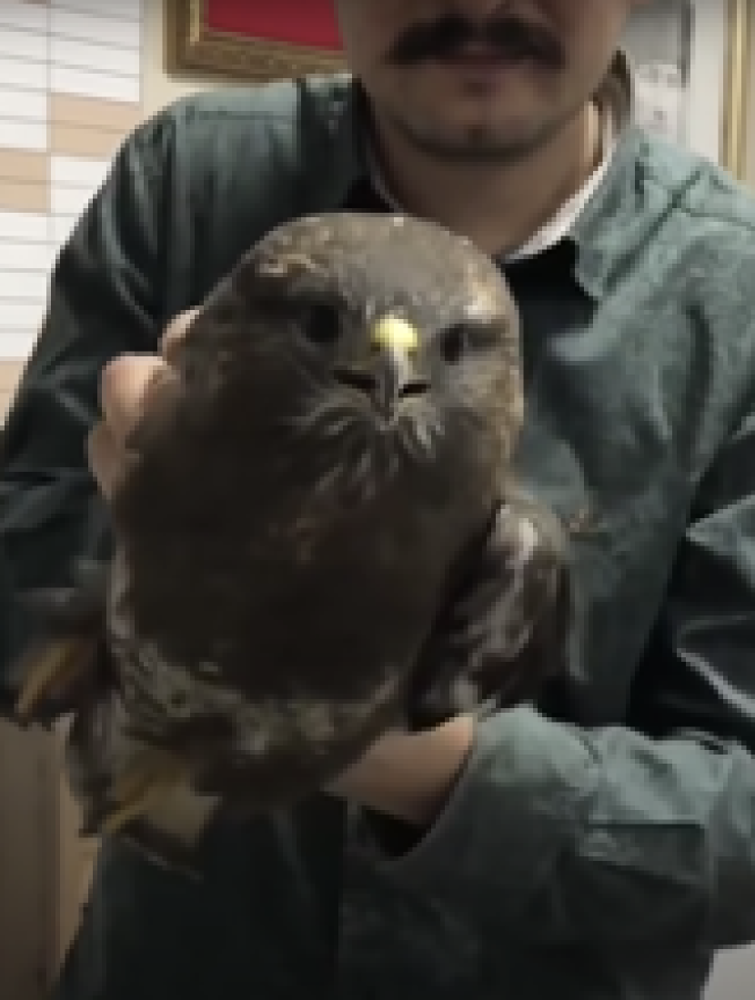
(a) start of video

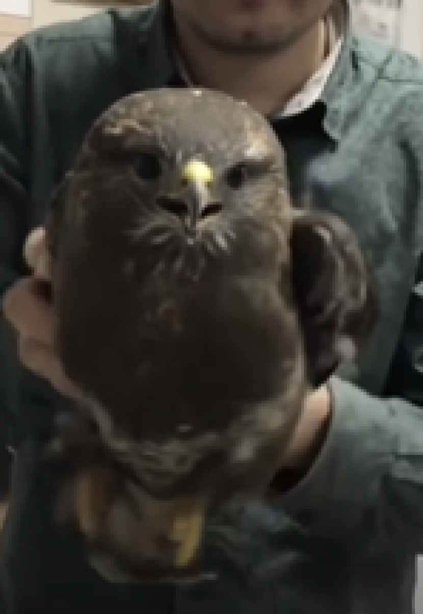
(b) midway

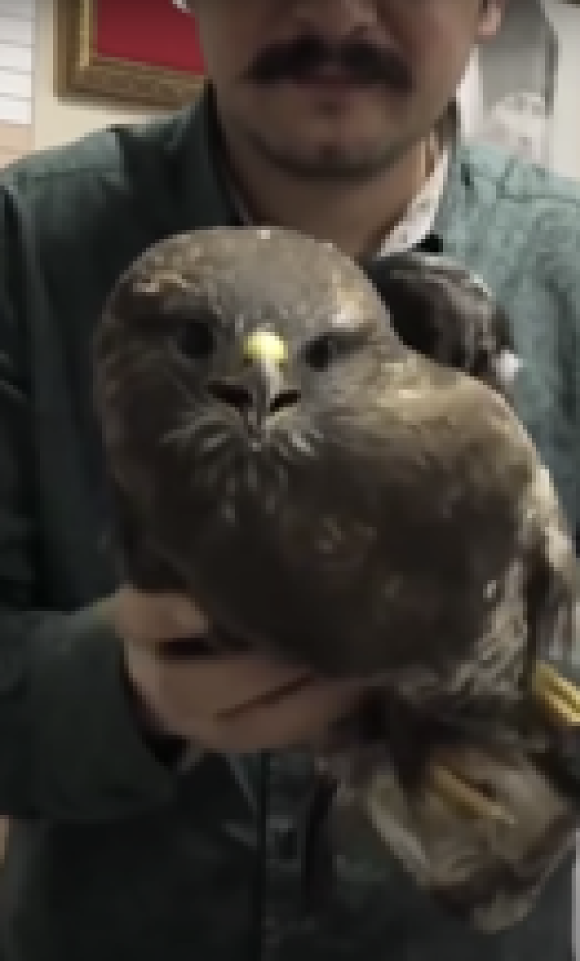
(c) end

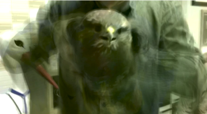
(d) Average of all images in video

Figure 2: Biological motion compensation. The position and the angle of the head of the hawk remain stable despite body motion to provide the hawk an stabilized vision. https://www.youtube.com/watch?v=aqgewVCC0k0

We are inspired by animal eyes that have fast mechanical movements that compensate for motion, in real-time and at high accuracy [1]. In Figure 2, we show frames $V(t)$ from a video of a hawk (Buteo jamaicensis) being moved by a human trainer [15]. We also show the average of the video $\sum_{t}\frac{V(t)}{T}$ over a time interval $T$. Note that the averaged image shows motion blurring, except where the eagle mechanically compensates for the shifts. We envision biologically-inspired motion compensation that happens during sensing. These sensors need to adaptively change their orientation, in real-time, and in concert with robot goals such as mapping or navigation. Effectively, the rotation matrix $R$ must cancel out robot motion to provide a ”stable” view of a scene.

I-B MEMS Mirror-enabled Adaptive LIDAR

The ability to reorient sensor pose could have many uses in robotics, particularly in image alignment during motion such as in SLAM. If the camera and robot are rigidly attached, then the camera experiences all the motion the robot experiences, including jitter and other potential disturbances that are detrimental to the Visual SLAM task. This could result in spurious features, errors in localization, and incorrect feature association leading to an inaccurate map. In this paper, we describe a sensor design that can perform image reorientation of a LiDAR in hardware without the need for any software processing for such compensation. Previously, pan-tilt-zoom (PTZ) cameras have attempted to address this problem. However, they use mechanical actuation which can react in ones of Hz making it not suitable for tasks such as egomotion compensation in real-time. This is evidenced by the limited use of PTZ cameras on robots - most robots just have sensors rigidly attached.

Our designs break through these past difficulties by exploiting recently available microelectromechanical (MEMS) and opto-mechanical components for changing camera parameters. Opto-MEMS components are famously fast (many kHz), and they allow the changing of the LiDAR projection offset orientation during robot motion, such that the view of LiDAR is effectively static. By changing LiDAR views two orders of magnitude (or more) faster than robot motion, we can effectively allow for camera views to be independent of the robot view. In this work, we can compensate the LiDAR point cloud using an onboard IMU or external feedback such as motion tracking setup. More generally, such compensation allows the robot to focus on the control task while the camera can perform perception (which is required for the control task) independently, and greatly simplifies robot planning as the planner does not need to account for perception and just needs to reason about the control task at hand.

MEMS LiDAR optics have the advantages of small size and low power consumption [44, 23, 24]. Our algorithmic and system design contributions beyond this are:

• We present the design of a novel LiDAR sensor adopting a MEMS mirror similar to this LiDAR MEMS scanner [49]. This design enables wide non-resonant scanning angles for arbitrary orientations. We integrate this with two types of feedback (IMU and external sensors) to demonstrate quick and high-rate motion compensation. Figure 1 shows the design of our sensor.

• We describe and geometrically characterize our sensor, showing that compensation in hardware can reduce the number of unknowns for proprioceptive and exteroceptive tasks. In a simulation, we characterize the effect of compensation delay and compensation rate to identify benefits for robot perception. The quantitative and qualitative results of these simulations are shown in Sect. III.

• We show UAV flight with a proof-of-concept hardware prototype combining external feedback with the MEMS mirror for egomotion compensation. We enable UAV flight by tethering the MEMS modulator to the other heavy necessary components, like the laser, photodetector, optics, the driver circuit, and the signal processing circuitry. The frequencies of the mirror modulation and IMU measurement are much higher than typical robot egomotion. Our prototype MEMS compensated scan system can perform such compensation in under 10 ms. Please see the accompanying video for proper visualization, and see Fig. 18.

• We provide an implementation of the sensor in the Gazebo simulator. Using this simulated sensor, we propose a framework to adapt modern LiDAR SLAM pipeline to incorporate motion compensation. We adapt a modern LiDAR SLAM pipeline LIO-SAM [39] to incorporate motion compensation to use such a sensor and demonstrate the utility of such motion compensation. We will open-source the sensor implementation, the UAV simulation environment, as well as our LIO-SAM adaptations on publication.

II Related Work

Small, compact LiDAR for small robotics: MEMS mirrors have been studied to build compact LiDAR systems [44, 23, 24]. For instance, Kasturi et al. demonstrated a UVA-borne LiDAR with an electrostatic MEMS mirror scanner that could fit into a small volume of 70 mm $\times$ 60 mm $\times$ 60 mm and weighed about only 50 g [23]. Kimoto et al. developed a LiDAR with an electromagnetic resonant MEMS mirror for robotic vehicles [24].

Comparison to software-based compensation: Motion compensation techniques and image stabilization techniques have been widely used in image captures. Similar to imaging devices, LiDAR point cloud shows point cloud blurring, motion artifacts caused by the motion of the LiDAR or the motion of the target object. Some software-based LiDAR motion compensation use ICP (iterative closest point) [32] and feature matching [12] to find translation and rotation of successive point clouds. Software-based compensation for robotics motion has been studied in great detail in SLAM algorithms [43] or Expectation– maximization (EM) methods[35]. Software-based motion compensation have a relative high computation barrier for micro-robotics and may degrade if the point cloud have large discrepancy. Some of the software-based motion compensation relies on the capture of a full frame of point cloud, so it cannot capture the motion frequency higher than the frame rate. For most of the LiDAR (other than flash LiDAR), especially the single scanning beam MEMS LiDAR, the rolling shutter effect caused by the LiDAR motion jitter remains a problem. In contrast to these approaches, we wish to compensate the sensor in hardware, during image capture. Hardware LiDAR motion compensation has several benefits. First, the compensation can be implemented to every LiDAR scanning pulse (for 2D MEMS based LiDAR), which can correct the rolling shutter effect and improve the motion response range. Second, the motion compensation algorithm very simple and can be implement on a low-power microcontroller or FPGA. Third, even if the hardware motion compensation still have some errors, it provides a better initialization for the following software compensation.

These ideas are closer to how PTZ cameras track dynamic objects [26, 19] and assist with background subtraction [40]. However, compared to these approaches, we can tackle egomotion of much higher frequencies, which is a unique challenge of micro-robots. We compensate signals much closer to those seen in adaptive optics and control for camera shake [2, 46, 3]. In addition, our system is on a free moving robot, rather than a fixed viewpoint.

Motorized gimbals: Comparing to motorized image stabilization systems [22], MEMS mirrors not only have smaller size and lighter weight, but their frequency response bandwidth are better than the bulky and heavy camera stabilizer. The MEMS mirror response time is can be less than 10 ms or even less than 1 ms. The servo motor of the camera stabilizer has a bandwidth width less than 30 Hz because they are bulky and have heavy load [28, 37]. This results in a response time higher than 10 ms.

Motion compensation in displays and robotics: Motion-compensated MEMS mirror scanner has been applied for projection, [13], where hand-shake is an issue. In contrast, we deal with the vibration of much higher frequencies, and our approach is closest to adaptive optics for robotics. For example, [42, 41] change the zoom and focal lengths of cameras for SLAM. We compensate using small mirrors, utilizing a rich tradition of compensation in device characterization[29] and to improve SNR [16]. Compared to all the previous methods, we are the first to show IMU-based LiDAR compensation with a MEMS mirror in hardware.

LiDAR SLAM: Ever since the seminal work of  [57], successive LIDAR SLAM designs largely follow a LiDAR SLAM architecture similar to Figure 10, where the front end consists De-skew and Feature extraction stages, while the backend usually consists of ICP and Pose Graph Optimization packages such as g2o [25] or GTSAM [8] that globally optimizes the odometry information as estimated by LiDAR visual odometry. Successive efforts moved towards improvement in the following sub areas: 1) tightly coupling LiDAR and IMU  [56]; 2) updating the backend PGO optimizer [39]; 3) updating the back end’s ICP  [33] [55]; 4) updating the front end’s point-cloud data structure to do away with ICP’s feature dependence [52] Nevertheless, to the best of our knowledge, all existing LiDAR SLAM systems are designed for LiDARs that are rigidly attached, via fixed joints, to robots and vehicles.

Sensor reorientation in Active SLAM: There has been a lot of work in the area of perception-aware path planning. A basic assumption of this line of work is that the sensor is rigidly attached to the robot, and therefore, its field of view can be changed only by changing the pose of the robot. [7][36][9] improve SLAM accuracy by actively changing the robot trajectory to improve the field-of-view. Our sensor can simplify these works by changing the FOV in hardware without requiring additional constraints on the path planning.

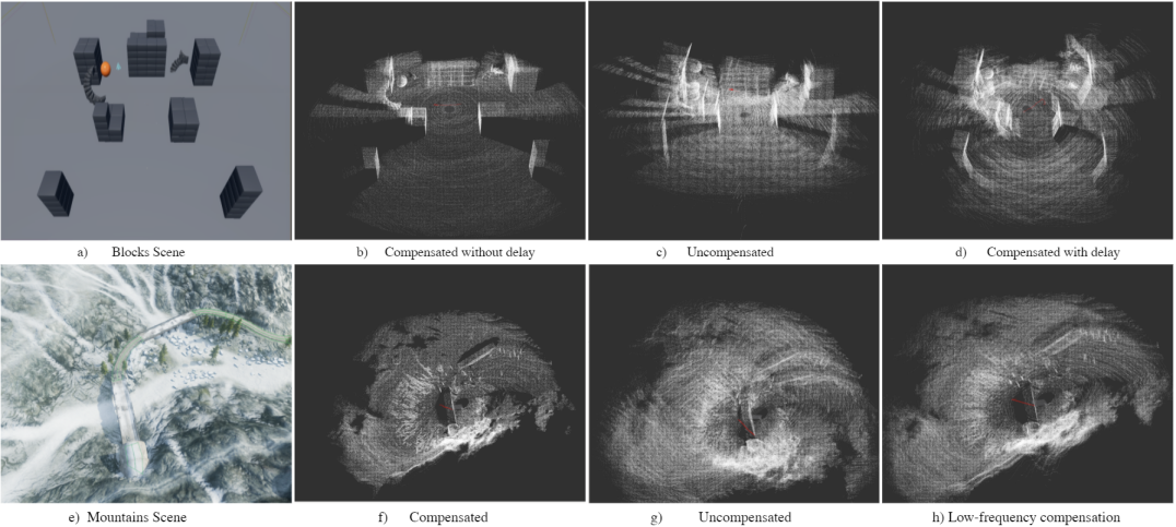
Figure 3: (a) Representative simulation scenario - Blocks scene (b) Mapping the Blocks scene with compensation at 55Hz and no delay (c) Mapping the Blocks scene without compensation (d) Mapping the Blocks scene with compensation at 55Hz and delay of 150ms. (e) Mountains scene (f) mountains scene simulation with 55Hz compensation and 0ms delay (g) mountains scene simulation without compensation. (h) mountains scene simulation with 5Hz compensation and 0ms delay.

III Understanding the Benefits of Compensated LiDAR in Simulation

III-A Basic LiDAR geometry

A MEMS-based LIDAR scanning system consists of a laser beam reflected off a small mirror. Voltages control the mirror by physically tilting it to different angles. This allows for LIDAR depth measurements at the direction corresponding the mirror position. Let the function controlling the azimuth be $\phi(V(t))$ and the function controlling the elevation be $\theta(V(t))$, where $V$ is the input voltage that varies with time step $t$.

To characterize our sensor, we use the the structure-from-motion (SFM) framework with the LIDAR projection matrix $\mathbf{P}$ and the robot’s rotation $\mathbf{R}$ and translation $t$

$$\mathbf{P}=\mathbf{K}\begin{bmatrix}\mathbf{R}&t\end{bmatrix}$$ (1)

Where $\mathbf{K}$ is an identity matrix.

In our scenario, the ‘pixels’ $\mathbf{x}$ relate to the mirror vector orientation $(\theta(V(t)),\phi(V(t))$ on a plane at unit distance from the mirror along the z-axis, and are obtained by projections of 3D points $\mathbf{X}$. Many robotics applications need point cloud alignment across frames, which needs us to recover unknown rotation and translation that minimizes the following optimization.

$$\min_{\mathbf{R},t}\|\mathbf{x}-\mathbf{P}\mathbf{X}\|.$$ (2)

This optimization usually happens in software, after LiDAR and IMU measurements [45]. Our key idea is that the MEMS mirror provides an opportunity to compensate or control two aspects of the projection matrix $\mathbf{P}$ before capture, in hardware.. In this paper, we propose to control a new aspect of the SFM equation in hardware: the rotation matrix $\mathbf{R}$. Given the robot pose (from onboard IMU or other sensing) and the intrinsic matrix, we can easily perform post-capture translation estimation.

$$\min_{t}\|\mathbf{x}-\mathbf{P}\mathbf{X}\|.$$ (3)

In other words, hardware compensation with MEMS mirrors simplifies the post-capture LIDAR alignment methods to just finding translation $t$, allowing for lightweight and low-latency algorithms to be used with minimal computational effort.

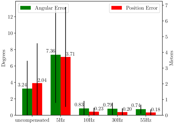
(a) Odometry error vs compensation rate (Blocks scene)

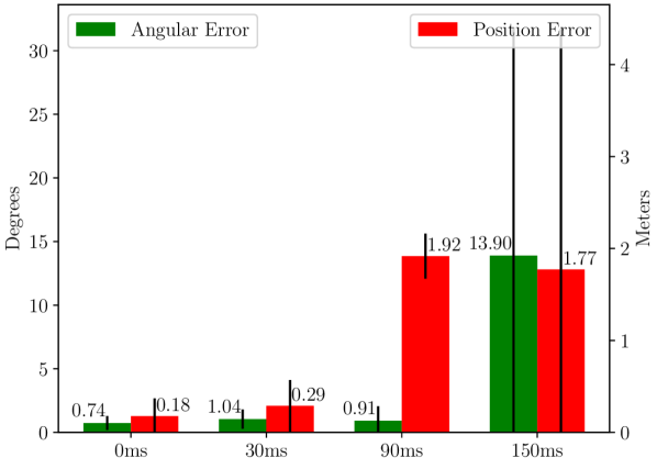
(b) Odometry error vs compensation delay (Blocks scene)

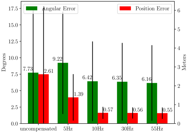
(c) Odometry error vs compensation rate (Mountains scene)

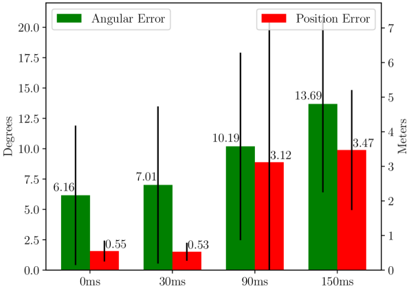
(d) Odometry error vs compensation delay (Mountains scene)

Figure 4: UAV odometry error while varying compensation rate and compensation delay in two scenes

III-B Benefits of IMU-compensated LiDAR in SLAM

We demonstrate the benefits of motion compensated LiDAR in simulation. Our setup is as follows - we use Airsim [38] running on Unreal Engine 4 for realistic perception and visualization. We tested two scenarios - a scene with geometric objects, called Blocks scene shown in Figure 3(a), and an outdoor scene with a bridge and mountains, called Mountains scene shown in Figure 3(e). In both scenes, the LiDAR is mounted on a prototype quadrotor UAV. We run LOAM [57], an open-source state-of-the-art LiDAR SLAM system to map the environment and localize the UAV.

As described earlier, motion compensation can be achieved through various means such as a gimble, active compensation of a pan-tilt-zoom camera or MEMS-based hardware compensation like our system. The differences between these methods are along two dimensions - (i) latency of compensation, called compensation delay from now on, and (ii) number of times we can compensate in a second, called compensation rate. By varying these two parameters in simulation, we compare each method’s performance. In order to systematically compensate based on IMU input, we perform some pre-processing of the IMU data. To smooth out the high angular velocity body movements, an angular moving average LiDAR stabilization algorithm is implemented. This method stores the past UAV orientations in a sliding, fix length queue, and reorients the mounted LiDAR towards the average of the past orientations. The average of the orientations is calculated through Linear Interpolation (LERP) of the stored quaternions. We detailed our calculations in Appendix.

The method is also known as Quaternion $L_{2}$-mean [14]. Given the relative short duration of the sliding window, and the relatively small range of rotation that’s cover during simulation flights, the prerequisite of using this method is met. It helps remove the impulsive jerky movements that may be observed by the LiDAR, akin to a low-pass filter.

In the experiment, the UAV performs three back-and-forth lateral flights between two way points. During the alternation of way points, the UAV reaches  130^∘/s in the X body axis. The mounted LiDAR is configured at 16 channels, 360 degree horizontal FOV, 30^∘ vertical FOV and with 150,000 Hz sample rate, akin to commercially available LiDARs.

To quantify performance, we calculate odometry error, the difference between the ground truth UAV positions and those positions estimated by LOAM. Figure 4 show the results from our simulations for Blocks scene and Mountains scene. We set the compensation rate to five different values - uncompensated, 5Hz, 10 Hz, 30 Hz, and 55 Hz. We set the compensation delay to five values - no delay (0 ms), 30 ms, 90 ms and 150 ms.

Both the position error and angular error are high when the compensation rate is uncompensated or 5 Hz in the Blocks scene (Figure 4(a)). It is significantly lower for 10 Hz, 30 Hz and 55 Hz. This shows that smaller rates of compensation as performed by a mechanical gimbal or a PTZ camera (which operate at 5 Hz or lower) are far less effective than a faster compensation mechanism such as the one proposed by us. Similarly, the error in position as well as orientation is low when the compensation delay is either 0ms or 30 ms (Figure 4(b)).

For larger compensation delays such as 90ms and 150 ms, the error is several times that of when the compensation delay is 30 ms. This shows that as the compensation delay is higher, as it could be with software-based compensation on low-power embedded systems, it is far less effective and leads to greater error in trajectory estimation. This further argues for a system such as ours that is able to perform compensation in hardware, and therefore at a higher rate. The trends are similar, albeit less pronounced in the Mountains scene where features are much less distinct and feature matching is more challenging in general. This proof-of-concept set of simulations encouraged us to build our proposed system.

IV Novel LiDAR Design

We propose a simple and effective design, where the MEMS mirror and photodetector are placed on a movable head. For image stabilization, we are also able to place the IMU there. A LiDAR engine and accompanying electronics are tethered to this device, which can be light and small enough for micro-robots. To enable both the LiDAR scanning and compensated scanning at high rate, it is important to understand the characterization of the MEMS scanner.

IV-A The MEMS mirror

All the compensation effects and size advantages described so far will be nullified if the MEMS mirror cannot survive the shock, vibration and shake associated real-world robots. Here we analyze the robustness of the MEMS mirror device for such platforms. Most MEMS mirrors rely on high-quality factor resonant scanning to achieve wide field-of-view (FoV), which leads to heavy ringing effects and overshoot with sudden changes of direction [30, 47]. A suitable MEMS mirror for motion-compensated scanning is expected to have a wide non-resonant scanning angle, smooth and fast step responses ,can operate under common robotics vibration and can survive shock. To achieve this goal, we adopt a popular electrothermal bimorph actuated MEMS mirror design [21, 48] to build this MEMS mirror. The employed MEMS mirror is fabricated with Al/SiO₂ based inverted-series-connected (ISC) bimorph actuation structure reported in [21]. This type of MEMS mirror has the advantages of simple and mature fabrication process [58, 50], wide non-resonant scanning angle, linear response and good stiffness. A new electrothermal MEMS mirror is designed and fabricated with the adaption of the motion compensation application. We note that other previously reported MEMS mirrors with electrothermal actuators, electrostatic actuators, or electromagnetic actuators may also be applicable to the motion compensated LiDAR scanning [23, 20, 49].

IV-B Compensation Algorithm

In the previous sections, we saw the advantages of MEMS mirror-based compensation and the feasibility for use in a robotic LiDAR. Here we focus on the details of the hardware-based rotation compensation algorithm using MEMS mirror scanning LiDAR and sensing for the compensation.

The MEMS mirror reflect a single ray of light towards a point in the spherical coordinate $\{\alpha,\beta,r\}$. The $\{\alpha,\beta\}$ are the two angular control input to the mirror to achieve such target. We will first establish the local(robot) and global (world) frames, then introduce known helper conversion from spherical to Cartesian coordinates, and finally gets into the details of compensation.

IV-B1 Coordinate Systems

Our LiDAR can compensate for rotation, but it can not compensate for translation. So all discussion here on in drops translation from $SE(3)$ and will only be focus on $SO(3)$. Let the robot have rotation $R_{robot}^{w}\in SO(3)$ relative to the world frame. In here, the frame of the un-moving base of the LiDAR sensor have Identity rotation $R_{base}^{w}\in SO(3)$ and therefore identical $SO(3)$ transformation as the robot frame. Let $R_{desired}^{w}\in SO(3)$ be the desired rotation target in the world frame. $R_{desired}^{w}$ can be decided by the users. For example, it can remain a constant rotation matrix, to impose a stabilization control policy and have the robot’s FOV to remain up-right. Other possibility includes aiming towards a specific world frame target $t\in R^{3}$ which we will touch on later, in  IV-B6.

IV-B2 Spherical-to-Cartesian Conversions

It is important to outline the conversion from the spherical, which is the control coordinate, to normal Cartesian coordinate. Points in the spherical coordinate $\{\alpha,\beta,r\}$ can be converted to Cartesian coordinate via known equations,

$$p_{cartesian}=\begin{bmatrix}x\\ y\\ z\\ \end{bmatrix}=\begin{bmatrix}r\cos{\alpha}\cos{\beta}\\ r\cos{\alpha}\sin{\beta}\\ r\sin{\alpha}\ \end{bmatrix}$$ (4)

and vice versa:

$$p_{spherical}=\begin{bmatrix}\alpha\\ \beta\\ r\end{bmatrix}=\begin{bmatrix}\arctan{\frac{z}{\sqrt{x^{2}+y_{M}^{2}}}}\\ \arctan{\frac{y}{x}}\\ \sqrt{x^{2}+y^{2}+z^{2}}\end{bmatrix}$$ (5)

Note that both $p_{cartesian}$ and $p_{spherical}$ are points located in the robot’s local coordinate frame, $R_{robot}^{w}$. Other literature’s refer to this frame as the local frame, or camera frame.

IV-B3 Spatial Scanning

A set of $i$ spherical control coordinates $\{\alpha_{i},\beta_{i},r_{i}\}$ defines the scanning pattern of the LiDAR, this is up to the user. For example, $\{\alpha_{i},\beta_{i}\}$ can be restricted to certain range to define a FOV limit. This range can span $(0,360)$ degrees like a commercially available velodyne LiDAR, or it can be smaller.

IV-B4 General Rotation Compensation

Let $R_{control}$ be the rotation from robot rotation $R_{robot}^{w}$ to the desired rotation $R_{desired}^{w}$ , therefore $R_{desired}^{w}=R_{control}R_{robot}^{w}$. We have,

$$R_{control}=R_{desired}^{w}(R_{robot}^{w})^{T}$$ (6)

Now, all points in the spatial scanning pattern $p_{spherical}=\{\alpha_{i},\beta_{i},r_{i}\}$ of the robot frame $R_{robot}^{w}$ can be re-projected to the desired frame $R_{desired}^{w}$, we first translate each $\{\alpha_{i},\beta_{i},r_{i}\}$ to Cartesian $p_{cartesian}$ by Equation 4. Then:

$$p_{desired-cartesian}=R_{control}p_{cartesian}$$ (7)

Then we can translate the rotated points $p_{desired-cartesian_{i}}$ back to the spherical coordinate $p_{desired-spherical_{i}}$, via equation 5 for point $i$’s control input.

It is important to note that, this full $SO(3)$ compensation is only achievable because our LiDAR project individual point $p_{i}$ independently from other points in the set. In the case of a traditional camera or a commercially available LiDAR like Velodyne, The entire set of $p_{i}$ can be viewed as being projected as a group and correlate to each other. In these other sensors, Full $SO(3)$ compensation is not achievable, even if the sensors are mounted to the robot by a universal joint with 2 degree of freedom $\alpha,\beta$. But we will also analyze this special case of grouped points re-projection, since our LiDAR can achieve this 2-axis only compensation.

IV-B5 Special Case: 2-axes only compensation

Let $R_{control}$ be limited to 2-axes rotation only:

$$R_{control}^{*}=\begin{bmatrix}\cos{\beta}&0&\sin{\beta}\\ 0&1&0&\\ -\sin{\beta}&0&\cos{\beta}\end{bmatrix}\begin{bmatrix}\cos{\alpha}&-\sin{\alpha}&0\\ \sin{\alpha}&\cos{\alpha}&0&\\ 0&0&1\end{bmatrix}$$ (8)

Our LiDAR can then use $R_{control}^{*}$ to perform 2-axis only compensation. Further, this compensation can be readily extend to commercially available cameras and LiDARs (such as Velodyne) mounted on a universal joint to the robot frame.

IV-B6 Target Aiming

Let $t_{target}^{w}\in\mathbb{R}^{3}$ be the target of interest in the world frame, and let $t_{robot}^{w}$ be the robot’s current world frame translation. Then

$$p_{aim}=t_{target}^{w}-t_{robot}^{w}$$ (9)

outlines the ray direction which we want to align our ”principle axis”, or the projection center point $p_{cartesian}:\{x=1,y=0,z=0\}$ towards. We can simply translate $p_{aim}$ to spherical coordinate via equation 5 to find $\alpha,\beta$, then compose a $R_{control}^{*}$ via equation 8 for the entire scanning grid.

IV-B7 MEMS Related details

MEMS-related details, relating to the 1-dimension controls of each actuation axis $\{\alpha,\beta\}$,  including analysis of robot motion shock on the MEMS as well as preliminary pointcloud stitching, are included in the appendix.

IV-C LiDAR Hardware Specifics

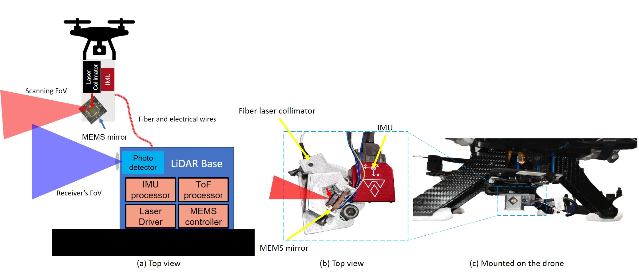
Figure 5: The movable LiDAR MEMS scanner head, which include the MEMS mirror, an IMU and a fiber laser collimator. (a) shows the top view and (b) shows the LiDAR scanner head mounted to the bottom of the UAV.

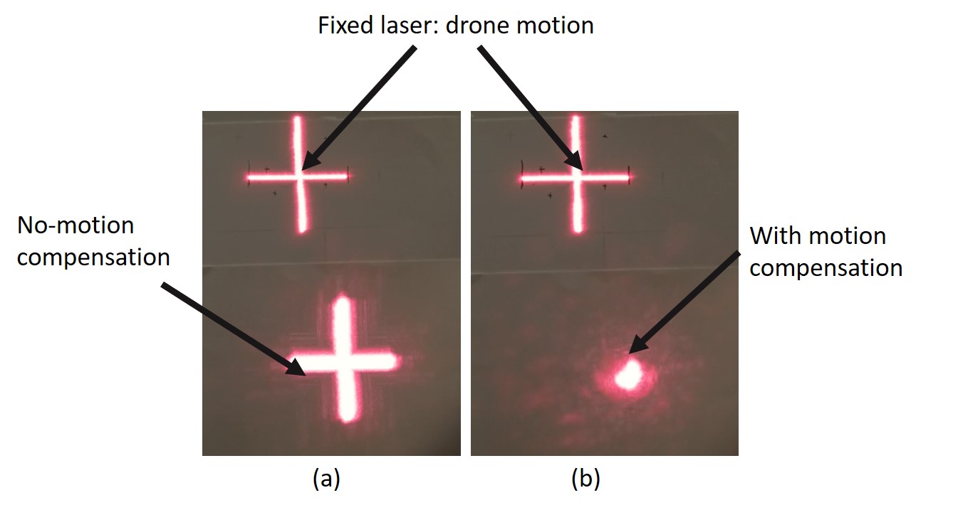
Figure 6: We use a visible laser to compare the effect of motion compensation of our sensor. The upper laser trace indicates UAV motion, and the lower laser trace indicates the compensated/uncompensated scanning laser reflected from the MEMS mirror. The compensated MEMS scanning (right) shows a much smaller laser trace area than the uncompensated MEMS scanning result.

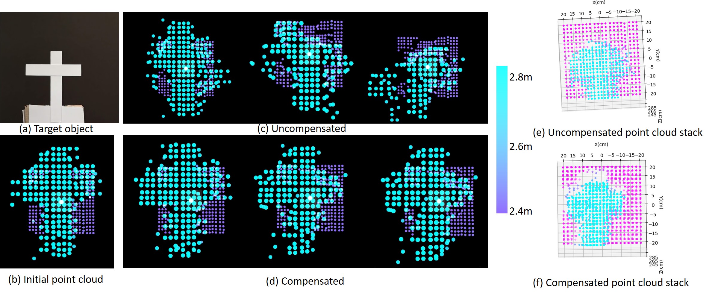
Figure 7: Motion compensated LiDAR point cloud result with hand held motion disturbance. (a)The target object ”+” placed 2.4 m from the LiDAR, along with (b), its initial point cloud scan. (c) and (d) show uncompensated vs. compensated scanning. Uncompensated shake range was $(-0.2^{\circ},+1.4^{\circ}),(+1.0^{\circ},+1.4^{\circ}),(-1.5^{\circ},+1.7^{\circ})$ and compensated shake range was $(-1.1^{\circ},+1.4^{\circ}),(+1.2^{\circ},-0.5^{\circ}),(-2.3^{\circ},+0.5^{\circ})$. (Please see supplementary video). (d and e) The stacking of 5 frame of point cloud of compensated and uncompensated results.

Our prototype (Figure 5) uses an InGaAs avalanche photodiode module (Thorlabs, APD130C). A fiber with a length of 3 m delivers the laser from the laser source to the scanner head. The gain-switch laser (Leishen, LEP-1550-600) is collimated and reflected by the MEMS mirror. The X-axis of the IMU (VectorNav, VN-100) is parallel to the neutral scanning direction of the MEMS mirror. The in-run bias stability of the gyroscope is $5-7^{\circ}$/hr typ. The scanner head sits on a tripod so that it can be rotated in the yaw and pitch directions. In the LiDAR base, an Arduino microcontroller is used to process the ToF signals, sample the IMU signals and control the MEMS mirror scanning direction. The data are sent to a PC for post-processing and visualization.

Since our motivation was use with micro-robots, our maximum detection distance is 4 m with a $80\%$ albedo object and the minimal resolvable distance is 5 cm. The maximum ToF measurement rate is 400 points/sec. According to the compensation algorithm described in the previous section, the MEMS mirror scanning direction is updated and compensated for motion at 400 Hz. We now describe our experiments. Please see the accompanying video for further clarification.

IV-D Compensation experiments with zero translation

To demonstrate the effect of compensation, a visible laser is used instead of the LiDAR IR light to visualize the effect of tracking. We mount the LiDAR MEMS scanner on the UAV, as shown in Figure 5. The MEMS mirror desired scanning angle is set to a single point on the target object ($0^{\circ}$ by $0^{\circ}$) to make it easier for comparing.

Here the entire scanning grid $\{\alpha_{i},\beta_{i},1\}$ consist of one single point only at the projection center. We use the general compensation outline in  IV-B4

The UAV together with the LiDAR scanner head is held with hand with random rotational motion in yaw/pitch direction. The upper laser trace comes from the laser rigidly connected to the UAV which indicates the UAV’s motion. The lower trace is reflected from the MEMS mirror, which shows the compensated/uncompensated scanning laser. The results are shown in Figure 6. The MEMS scanning laser trace area of the compensated scanning is significantly smaller than the uncompensated scanning trace under similar rotational motion disturbance. The videos of the real-time compensation results is available in the supplementary materials.

Then the IR pulse laser is connected to run the LiDAR. An object of interest (in the shape of a +) is placed 2.4 m away from the LiDAR and at the center of the field of view and the background is at 2.8 m, as shown in Figure 7(a). The MEMS mirror performs a raster scanning pattern with an initial field of view of $-3.5^{\circ}$$\sim$$+3.5^{\circ}$ in both axes to leave the room for compensation. Each frame has 20 by 20 pixels, and the frame refresh rate is 1 fps. To mimic robot vibration, the tripod is rotated randomly in the directions of yaw (Z-axis) and pitch (Y-axis), and the point clouds are shown in Figures 7(d). Despite the motion of the LiDAR head, the point clouds are quite stable. The differences among all of the point clouds are generally less than 2 pixel in either axis, caused by measurement noise.

Figure 7(c) shows the point clouds without compensated scanning, where the relative positions of the target object in the point clouds keep changing. The target object may come out of the MEMS scanning FoV without compensation. With a continuous rotation of 1.5 Hz in the Y-axis, the same structure may appear in multiple positions in the same frame of the point cloud, as shown in the 3rd figure of Figure 7(c). Multiple frames of point cloud are stocked together and shown in the last column of Figure 7. The object can still be identified in the compensated point cloud (Figure 7(f)), but becomes fuzzy caused by the motion jitter when not compensated (Figure 7(e). The videos of the real-time compensation point cloud results is available in the supplementary materials.

V UAV Experiment

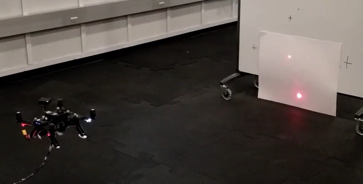
(a) Our UAV setup with Intel Aero UAV and our LiDAR mounted on it.

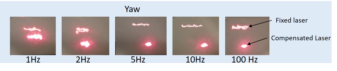
(b) Effect of compensation rate on yaw rotation

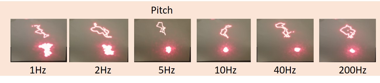
(c) Effect of compensation rate on pitch rotation

Figure 8: A comparison of the compensation strength versus the robot pose sampling frequencies. All the images are accumulation of 12s of UAV hovering videos. The compensation target scanning direction is a fixed direction.

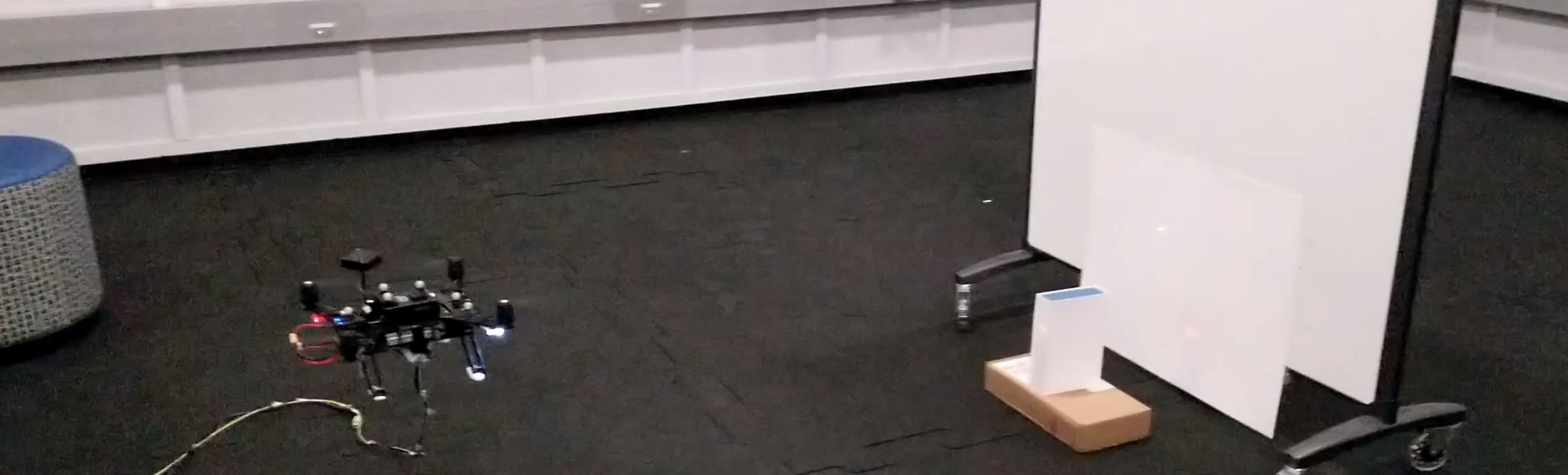
(a) Our set up with UAV, LiDAR and the feature target.

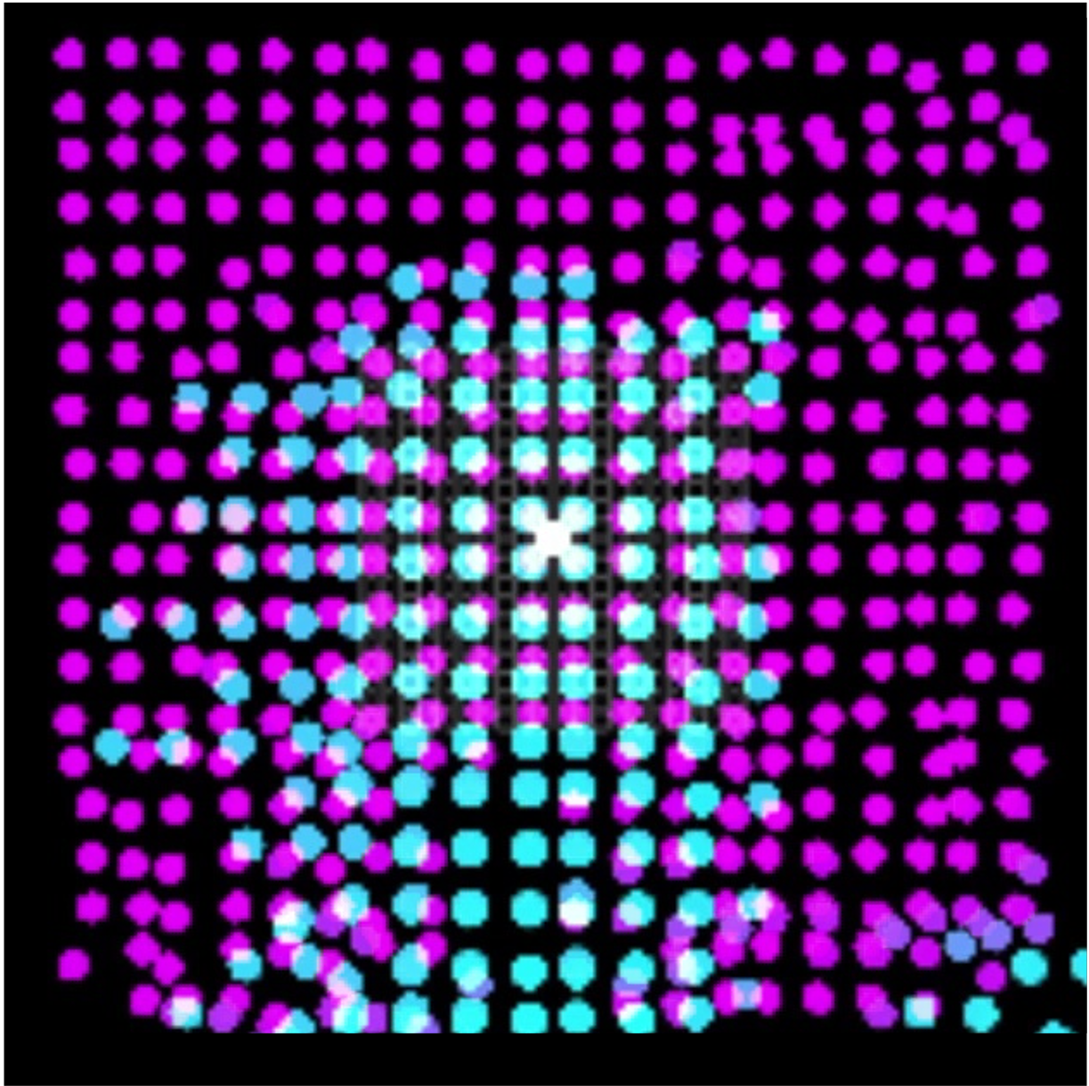
(b) Uncompensated

(c) One frame

(d) 50Hz sampling rate

(e) 2Hz sampling rate

(f) 1Hz sampling rate

Figure 9: A comparison of the compensation strength verse the IMU sampling frequencies. The images are accumulation of 20s of point cloud video during the UAV hovering. We use a cuboidal object (as seen in Figure 9(a)) as object of interest. The width of the target increases due to compensation inaccuracy as we reduce compensation rate from 50 Hz to 1 Hz demonstrating the utility of high rates of compensation even in such static scenarios

Next, we demonstrated the motion compensated LiDAR by flying it on a UAV. The robot pose is from an external motion capture system that tracks the UAV. We vary the robot pose sampling rate and study its effect on the effect of compensation. The UAV is controlled to hover at a designated position with yaw/pitch rotation as motion jitter. Motion compensated LiDAR is set to compensate all the rotational motion, including the controlled rotation and the random motion disturbance. The compensated MEMS scanning laser uses a visible light, and the other visible laser is fixed at a relative higher position on the UAV, as shown in the images in Figure 8(b). The target scanning direction is a fixed point on the target.

Here, the entire scanning grid $\{\alpha_{i},\beta_{i},1\}$ consist of 20x20 grid pattern points. We use the aiming compensation outline in  IV-B6

We trim about 12 s videos in each experiments while the UAV is flying, and the each frames of the videos are accumulated into an image to track the motion of the UAV and the errors of the compensated scanning.

The robot pose sampling rate is set from 1 Hz to 200 Hz to investigate its effect on the compensation results. The controlled UAV rotations are in the yaw and pitch direction. However, the actual motions cause some random motions during the flying. Point clouds are also collected when the UAV is hovering and we overlap several frames. As the robot pose sampling frequency increases from 1Hz, 2Hz to 50Hz, the width of the overlapping area shrink from 10 to 11 points at 1Hz (Fig. 9(f)), to 6 points at 50 Hz (9(d)). As the target object in the size of the target object in the point cloud settle down to the a smaller area and the location of the target in the point cloud becomes more certain.

VI Rotation Compensated LiDAR-Inertial SLAM Design

SLAM is a body of fundamental applications for visual sensors. All exisitng SLAM literatures reason about its odometry in the sensor’s local frame, sometimes call camera frame. In this work this frame is the robot frame, with world frame orientation $R_{robot}^{w}$, refer to  IV-B1.

The basic assumption of the existing SLAM is that visual sensor readings use the robot frame with world rotation $R_{robot}^{w}$ as their reference. This assumption is untrue for our sensor, because that our sensor readings use the frame with world orientation $R_{control}R_{robot}^{w}$ as their reference.

Through sections  IV-B4 to IV-B6, the additional none-zero rotation $R_{control}$ orients the original scanning grid towards different directions. The existence of $R_{control}$ breaks the basic assumption of existing SLAM.

$R_{control}$ must be compensated for, in order for the existing SLAM pipelines to work with our sensor. This can be done post-capture, we can use either  IV-B4 or  IV-B5 to compensate. We details the compensation later in  VI-B.

Most LiDAR odometry pipelines utilize Iterative Closest Point (ICP) to match consecutive scans and determine the rotation and translation between the poses. Any rotation of the LiDAR relative to the vehicle would cause errors in the ICP’s prior. This would directly impact the quality of ICP’s point-cloud registration. Although ICP can tolerate certain levels of error in its prior, in Section VI-C2 we will show that it is far from enough when the magnitude of $R_{control}$ input increases.

VI-A Motion Compensation for LiDAR SLAM

In this simulation, we simulate a 360 degree velodyne LiDAR, that can rotate relative to the vehicle it is mounted on, by a universal joint. A universal joint has rotational DOF similar to a MEMS mirror, both limited to 2 DOF. This setup fits into the compensation framework introduced in the special case  IV-B5. In this section, we will demonstrate in simulation that such rotation introduces error in an off-the-shelf LiDAR SLAM pipeline. Additionally, We propose a general method to incorporate such rotation into consideration when performing LiDAR-related SLAM. We demonstrate the effectiveness of the framework in a Rotation Compensated LiDAR-Inertial Odometry and Mapping package, which is publicly available on  Github.

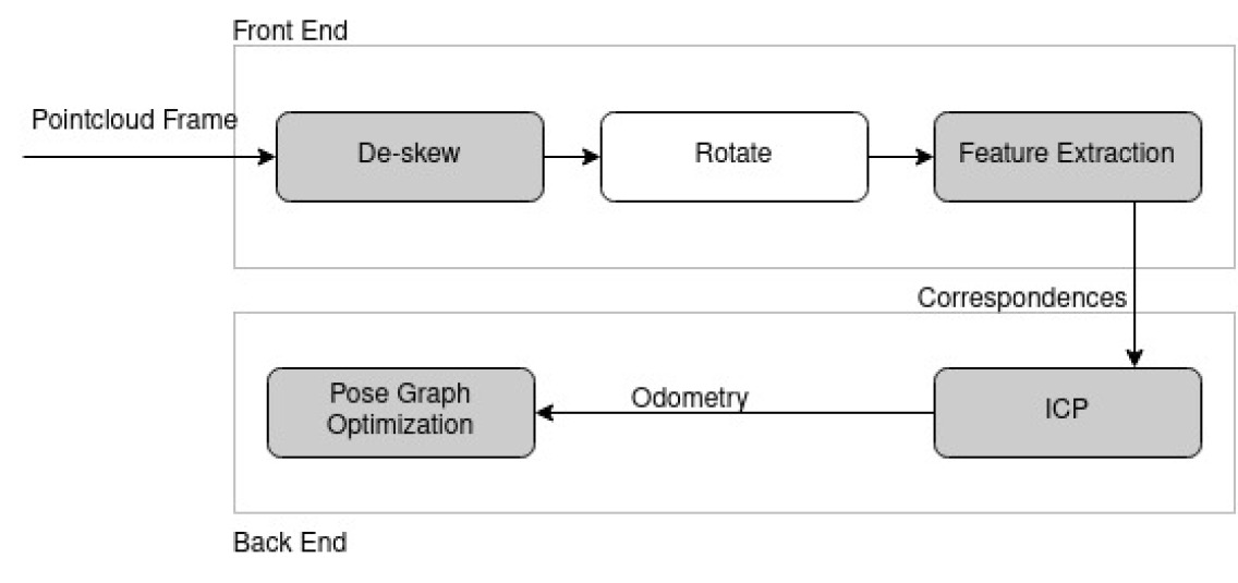
Figure 10: Illustration of our rotating LiDAR SLAM augmentation pipelines. The existing structures are shown in grey

For the ease of integration, our framework proposal does not make large edits in the existing paradigm. It only adds a “rotate” stage right after the de-skew stage in the front end, and before feature extraction stage. This edition can be easily integrated with existing pipeline and future designs. The rotate stage does one single operation, it rotates the de-skewed point cloud according to the control rotation input to the LiDAR. Our workflow block diagram in shown in Figure  10.

VI-B The Rotation Stage

The purpose of this stage of the pipeline, is to rotate the captured LiDAR frame, to a correct position, relative to the LiDAR’s base frame of reference. (In this work, the LiDAR’s base frame is identical to the vehicle’s body frame.)

Let the Lidar’s base frame have world rotation $R_{robot}^{w}\in SO(3)$.

In a traditional LiDAR that doesn’t rotate, all points received in a LiDAR frame are position relative to the LiDAR’s base frame, with world rotation $R_{robot}^{w}$. However, this assumption is incorrect for our device, where the LiDAR frame is positioned relative to the frame with rotation $R_{control}R_{robot}^{w}$.

The LiDAR’s head can rotate $R_{control}\in SO(3)$, relative to its base. This rotation is restricted to azimuth $\beta$ and elevation directions $\alpha$. note that in here we analyze a more generalize, special case compensation IV-B5, but the it can be easily extend to full $SO(3)$ compensation IV-B4,

When a LiDAR frame is received, we take the most recently known rotation $\alpha,\beta$, in this case the most recent known command rotation, and converts them into a rotation matrix:

$$\color[rgb]{0,0,0}R_{control}\color[rgb]{0,0,0}=\begin{bmatrix}\cos{\beta}&0&\sin{\beta}\\ 0&1&0&\\ -\sin{\beta}&0&\cos{\beta}\end{bmatrix}\begin{bmatrix}\cos{\alpha}&-\sin{\alpha}&0\\ \sin{\alpha}&\cos{\alpha}&0&\\ 0&0&1\end{bmatrix}$$ (10)

And applies the rotation to each point $p\in\mathbb{R}^{3}$ in the frame point-cloud:

$$p_{rotated}=\color[rgb]{0,0,0}R_{control}\color[rgb]{0,0,0}p$$ (11)

The rotated point-cloud $p_{rotated}$ now locates at the correct position, relative to the LiDAR’s base frame, with world rotation $R_{robot}^{w}$. The basic assumption of traditional SLAM are now met.

VI-C Evaluation

Now we evaluate the sensor in simulation to answer a few questions. First, we want to compare traditional LiDAR SLAM and our Motion Compensated SLAM in terms of the handling change in mirror/universal joint orientation magnitude. Next we investigate the effect of noise in the mirror’s orientation (say through a faulty IMU or other sensor) on the robustness of our pipeline. We also show the degree to which our pipeline can tolerate such noise.

The proposed SLAM framework should be expected to function, even when the LiDAR users employ control policies that rotate its FOV significantly frame-to-frame. This is Unlike the scenario of running a active stabilization control policy proposed in  III-B, Where frame-to-frame variation is minimal. Therefore, in this evaluating section, we use control policy that samples random LiDAR rotation control input from Gaussian distributions at high frequency.

We choose LIO-SAM as the traditional SLAM package to compare against, and built our Motion Compensation framework into it, and open-source it on github. LIO-SAM has all the signature point-cloud processing stages shown in Figure  10. It is relatively new and has good SLAM accuracy performance versus State-of-the-Art. We hope through the open-source code we can demonstrate to the community an example of incorporating our framework.

For Odometry error evaluation, We calculate Average Translation Error (ATE) which is defined by the KITTI benchmark  [11]:

$$E_{trans}(\mathcal{F})=\frac{1}{|\mathcal{F}|}\sum_{i,j\in\mathcal{F}}\|\hat{T}_{j}\hat{T}_{i}^{-1}(T_{j}T_{i}^{-1})^{-1}\|_{2}$$ (12)

Where $\mathcal{F}$ is a set of frames $(i,j)$, $T$ and $\hat{T}$ are the estimated and true LiDAR poses respectively.

VI-C1 Experiment Set Up

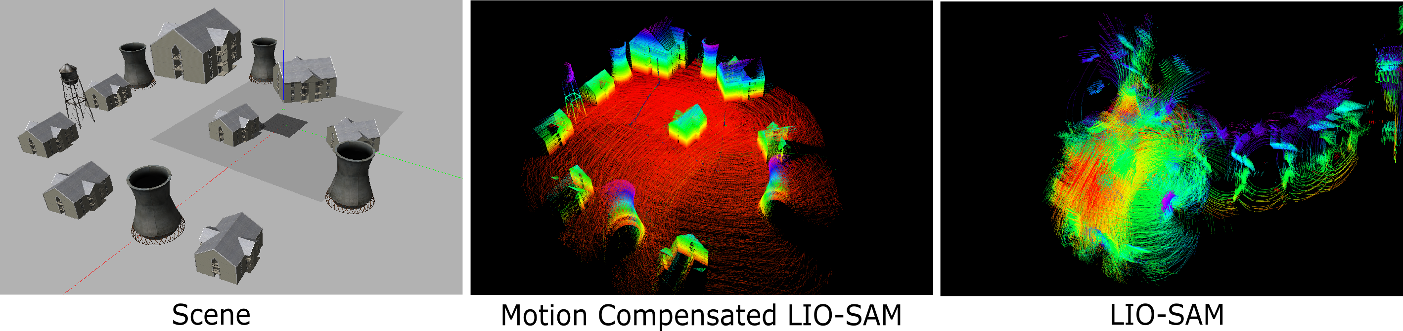
Figure 11: Illustration of a) our simulator environment, b) mapping results on LIO-SAM with our motion compensation c) mapping results on stock LIO-SAM. It is worth noting that the pointcloud generated from the simulation has rotation with respect to the frame with world rotation $R_{control}R_{robot}^{w}$, which breaks any traditional visual SLAM’s assumption, see section VI. It has significant frame-to-frame FOV variations (See section  VI-C), which is difficult for any un-compensated, traditional SLAM to handle.

A simulation study is setup in robotics simulator Gazebo, where a LiDAR with similar sensor characteristics to a VLP-32  [velodyne] is mounted on a simulated drone. Further, the LiDAR can rotate in azimuth and elevation via a universal joint. The simulated drone iris, is from the PX4’s simulation package. Its onboard IMU have noise added to it according to a noise model outlined in Kalibr  [10]. The point-cloud messages from the LiDAR, as well as the IMU messages from the drone, are passed into robotics middleware ROS, where the proposed LiDAR SLAM package runs. The drone is commanded to flight in a diamond waypoint pattern, around a enviornment with different types of resident buildings.

The proposed LiDAR-Inertial SLAM package builds on top of LIO-SAM, which employs the powerful PGO backend GTSAM  [8]. We incoporate the compensation described in VI-B into LIO-SAM, here on in refer to as Motion Compensated LIO-SAM. Naturally, we will compare SLAM performance of Motion Compensated LIO-SAM, against the stock version of LIO-SAM. See Figure  11. To control the orientation of the universal joint, angular commands in $\alpha,\beta$, in degrees, are input to the mirror.

VI-C2 Level of mirror control orientation magnitude tolerable by an unmodified pipeline vs our system

The two angular commands are sampled from 1-d Gaussian distributions with standard deviation of various degrees, at 10 Hz. Odometry error vs command rotation’s gaussian standard deviation is plotted in figure 12. An Gaussian distribution with 8 degree standard deviation generate input angle within +-,8,16,24 degrees, 68,95 and 99.7 percent of the time respectively. Therefore 99.7 percent of the time, angular input span a range of 48 degrees.

In short, by considering mirror rotation, the system can tolerates angular input that span 48 degrees. In contrast, without mirror rotation information, the system can only tolerate angular input that span 12 degrees.

Even in the cases where the input spans less than 12 degrees, by considering mirror rotation, SLAM quality improves in comparison.

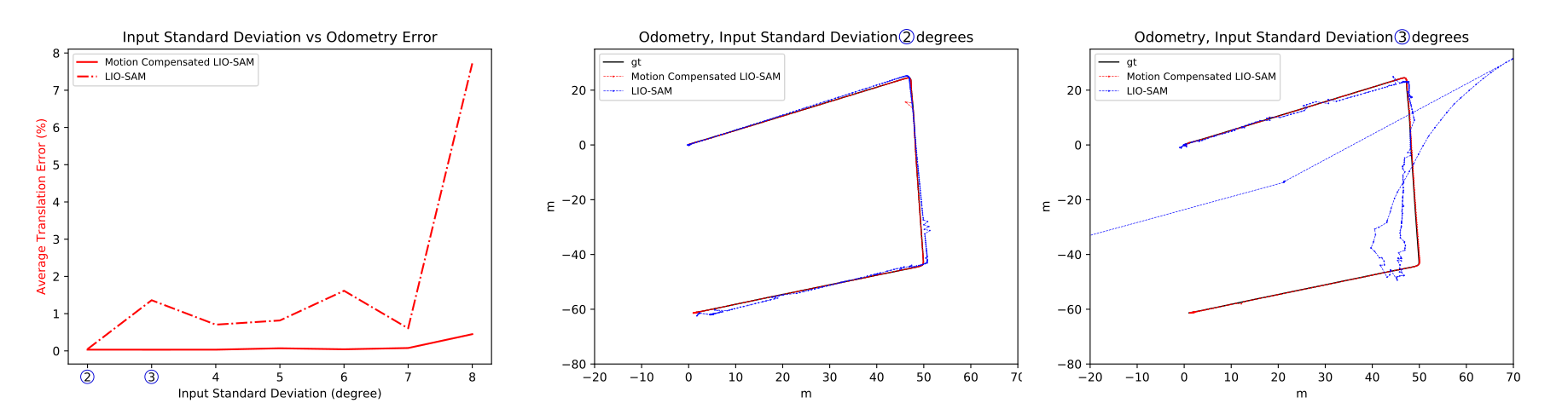
Figure 12: a) Mirror control magnitude and odometry error, Our Motion Compensated LIO-SAM vs LIO-SAM . As mirror control magnitudes increase, the unmodified LIO-SAM fails completely. b) At 2 degrees standard deviation, Our Motion Compensated LIO-SAM outperforms LIO-SAM c) At 3 degrees standard deviation, degree threshold and beyond, Our Motion Compensatedd LIO-SAM perform normally while the stock LIO-SAM completely fails

VI-C3 Level of mirror control noise tolerable

The two angular commands are sampled from 1-d Gaussian distributions with standard deviation of 3 degrees. Additionally, Noise rotations in both azimuth and elevation are added on top of each channel. Odometry error vs command rotation’s noise Gaussian standard deviation is plotted in Figure 13. The system can tolerate mirror input control noise up to 1.6 degree standard deviation, which spans 9.6 degree.

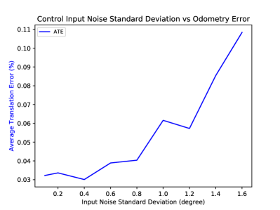
Figure 13: Mirror control noise and odometry error. As the mirror control noise increases, the odometry error also increases. Our pipeline fails after noise standard deviation exceeds 1.6 degree.

VII Limitations and Conclusions

We have designed an adaptive lightweight LiDAR capable of reorienting itself. We have demonstrated the benefits of such a LiDAR in simulation as well as experiment. We have demonstrated in experiment image stabilization in hardware using an onboard IMU. We have also demonstrated viewing an object of interest using this LiDAR through external robot pose feedback. Please see the supplementary material of this paper for some MEMS-related details, including analysis of robot motion shock on the MEMS as well as preliminary point cloud stitching. We also explain how such a sensor can reduce sensing uncertainty. Finally, our accompanying video shows our experiments in action.

We would also like to acknowledge limitations of our study.

• We have indirectly compared to software methods using compensation delay. This is because, compared to hardware-compensation, any software-compensation will add delay, and therefore delay is a fundamental metric for hardware-software comparison. For future work we will directly compared with software compensation methods.

• Our design requires the robot to connected to the heavier sensing components using a tether. This limits the fly range and the detection FoV of the system. Although removing the tether restriction is left to future work, we believe that our design is capable of advancing sensing in microrobots significantly, and will help our community in designing microrobots in the future.

• All our results (using IMU as well as Vicon motion capture) are indoor results. We hope to perform future experiments with outdoor effects such as wind.

• In our current system design, there are implementation bottlenecks that limit compensated bandwidth. These are caused by the MEMS mirror and by the signal processing. Tightly coupled on-board designs can reduce these.

In conclusion, through simulation and a prototype implementation we realize our design shown in Fig 1. We have shown, in simulation on on real hardware experiments, that hardware-compensation using a MEMS mirror improves both reconstruction and mapping. In particular, microrobots which suffer from heavy vibration and motion jitter (such as flapping-wing MAVs [51]) can benefit greatly from the motion compensated MEMS mirror scanning LiDAR for stabilized scene capture. Finally, over the long term, we believe that our design methodology can decouple robot and sensor geometry greatly simplifying robot perception.

velodyne

Supplementary materials

Motivation

Fisher Information in Iterative Closest Point

A popular method for 3D feature alignment is Iterative Closest Point method. In feature-based ICP, the uncertainty of robot pose estimation is inversely correlated to the amount of correctly matched features being observed. Recent work has reasoned about this using the Cramér–Rao lower bound; regardless of their parameterizations, these come in very similar form. We refer the readers to [5] and [59] for detail.

Consider a robot equipped with LiDAR sensor in the environment. Each beam of the sensor is represented as a bearing vector measurement, which is a vector to the direction of the ray, whose length is generated by ray-tracing measurement model, corrupted by zero-mean Gaussian noise. Let the LiDAR‘s pose be $\boldsymbol{p}\triangleq(\boldsymbol{R},\boldsymbol{t})$ w.r.t a fixed world frame. This sensor output $\boldsymbol{z}$ of $m$ bearing vector measurements, but only $n$ of them are correctly matched to environmental features. In [59], a 3D featured matching paper where parameterizations of the measurements are in bearing vectors, the FI is expressed (within identical and independent zero-mean Gaussian noise $\mathcal{N}(0,\sigma^{2})$) as

$$I_{\boldsymbol{p}}(\boldsymbol{z})=\frac{1}{\sigma^{2}}\sum_{i}^{n}I_{i}$$ (13)

Where $I_{i}$ stands for the Fisher Information Matrix associated with the i-th matched 3D feature bearing vector measurement.

In Equation 13 the FIM in feature-based ICP is positively correlated to the amount of correctly matched features observed. In other words, the Cramér–Rao lower bound is inversely correlated to the amount of correctly matched features. Basically, the more correctly matched features are considered, the lower the odometry uncertainty is. While the above is hardly surprising, it forms the theoretical backing for our system design where we hypothesize that decoupling increases correctly matched features because the sensor can orient towards feature rich regions.

VII-A Quaternion $L_{2}-mean$

Supposedly $q_{1}.....q_{n}$ are the world frame quaternions store in a queue data structure, representing the UAV’s world frame rotation in the last $n$ time stamps. We can find its average via LERP, summing and normalizing the quaternions as 4-vectors:

$$q_{avg}=\frac{\sum_{i=1}^{n}q_{i}}{||\sum_{i=1}^{n}q_{i}||_{2}}$$ (14)

$q_{avg}$ can be converted into a rotation matrix $R_{desired}^{w}$. Then we can find $R_{control}$ and the control input of each compensated point in the spatial scanning set according to methods outline in  IV-B4.

Motion Compensation Controller

The IMU model is provided by the manufacturer, and it is usually simplified as a passive low-pass filter model. For example, the IMU(VN-100) has a bandwidth of $f_{2}=150$Hz with a simplified transfer function of

$$H_{2}(s)=\frac{\frac{f_{2}}{2\pi}}{s+\frac{f_{2}}{2\pi}}$$ (15)

The compensating components $H_{g}(s)$ and the high pass filter $H_{pf}(s)$ improve the usable range of the motion compensation. We assume that the relative low frequency spectrum motion is the desired motion, and should not be compensated. It can be achieved by tuning the bandwidth of the high pass filter $H_{pf}(s)$. In this work, a passive high pass filter with a bandwidth of $f_{h}$ is selected,

$$H_{pf}(s)=\frac{s}{s+2\pi f_{h}}$$ (16)

To improve the response bandwidth at higher frequency and suppress the noise, $H_{g}(s)$ is added. The $H_{g}(s)$ is defined with the inverse of the transfer function of the IMU and the MEMS mirror,

$$H_{g}(s)=\frac{B(s)}{H_{1}(s)\dot{H}_{2}(s)}$$ (17)

where $B(s)$ ensure that the order of the numerator is not higher than the order of the denominator. A fourth order Butter-worth filter with a bandwidth of $f_{B}=200$Hz is used as the low pass filter. The 200 Hz bandwidth is selected to improve the speed while it can still suppress the resonance of the MEMS mirror, which is,

$$B(s)=\frac{1}{\frac{s}{2\pi f_{B}}^{4}+2.613\frac{s}{2\pi f_{B}}^{3}+3.414\frac{s}{2\pi f_{B}}^{2}+2.613\frac{s}{2\pi f_{B}}+1}$$ (18)

which implies,

$$H_{g}(s)=\frac{s^{4}+512s^{3}+1.081e08s^{2}+1.486e11s+4.457e13}{4.457e13}$$ (19)

To implement the transfer function in a microcontroller, the continuous-time transfer function $H_{g}(s)$ is translated to a discrete-time transfer function $G[z]$ with a sampling time of 0.0025s,

$$G[z]=\frac{Y[z]}{X[z]}=\frac{0.843z^{4}+0.93z^{3}-0.32z^{2}-0.045z+0.0064}{z^{4}+0.32z^{3}+0.11z^{2}-0.017z+0.0021}$$ (20)

$X[z]$ in the input (IMU measurement) and $Y[z]$ is the output (MEMS scanning angle) in the $Z$ domain. Converting the discrete-time transfer function $G[z]$ to the time domain,

$$y[n]=(0.843x[n]+0.93x[n-1]-0.32x[n-2]-0.045x[n-3]\\ +0.0064x[n-4])-\\ (0.32y[n-1]+0.11y[n-2]-0.017y[n-3]+0.0021y[n-4]).$$ (21)

Simulink is used to simulate the performance of the controller and tune the parameters. The Simulink setup is shown in Fig. 14. The input motion jitter is a sinusoid wave. Fig. 14(b) and (c) shows the motion compensation residues with the input motion jitter frequency of 5Hz and 10 Hz. $H_{g}(s)$ can effectively reduce the residue. Note that the compensation residue is expected to be better than real-world experiments because of the digitization.

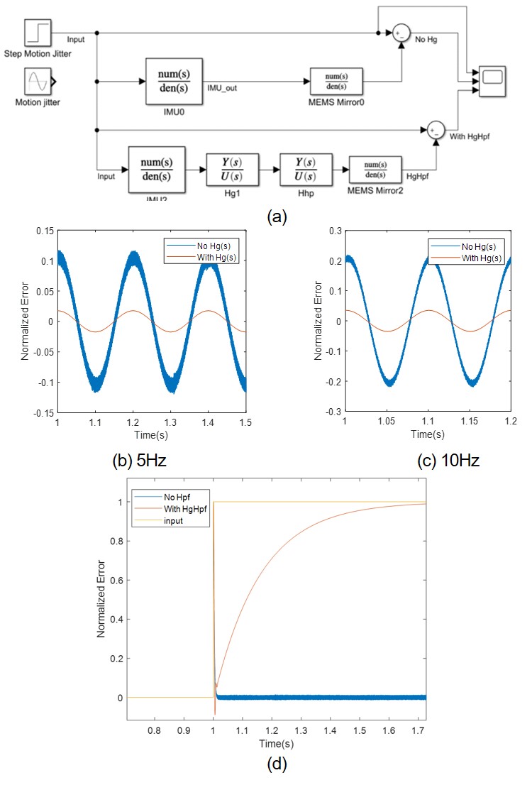
Figure 14: (a) The Simulink simulation setup of the motion compensation. The input frequency is 5 Hz (b) and 10 Hz (c). (d) The effect of $H_{pf}(s)$ under step response.

Motion Compensation Controller Design

Those algorithms provide motion-compensated MEMS scanning in steady-state. However, as both the IMU and the MEMS mirror have limited response bandwidths, the residue and the speed of the motion compensation may get worse as the frequency of motion jitter increases. Also, the MEMS mirror has a limited scanning range, so the range of motion compensation is also limited. Since the motion compensation system is an open-loop system, a compensating stage $H_{g}(s)$ can be added to the microcontroller to increase the performance of the system.

A simplified block diagram of the open-loop motion compensation system is shown in Figure 15, where $H_{1}(s)$ denotes the MEMS mirror tip-tilt model given in Eq. 22, $H_{2}(s)$ is the IMU model, $H_{g}(s)$ is the compensating components, $H_{pf}(s)$ is an optional high-pass filter and $F$ is the model for the MEMS mirror driver.

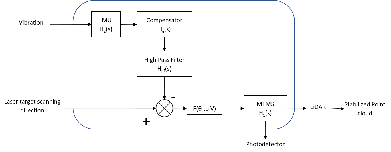
Figure 15: The block diagram of the open-loop motion compensation system.

Motion Compensation Strength with motion jitter frequency

The MEMS mirror motion compensation system is controlled by an Arduino Mega. The IMU sends the data to the Arduino at 400 Hz. The data is processed, and the compensator $H_{g}(s)$ is implemented by the Arduino to get the MEMS angle and the desired driving voltages of the MEMS mirror. The two MEMS orthogonal scanning directions are assembled parallel to two IMU axes. To evaluate the compensation results, the reflected laser is captured by a PSD (position-sensitive detector) sensor fixed on the bench. The PSD sensor is placed 12 cm from the MEMS mirror. The PSD is for compensation evaluation only and is not in the controller loop.

Testing was done only on LEVEL 1 and 2, since high-resolution translation measurement is not available, so LEVEL 3 compensation cannot be tested. The motion-compensated MEMS scanner test is assembled on a step motor to test the compensation capability under various frequencies. The test bench, including the MEMS mirror, the IMU, and the pigtailed laser are fixed on the shaft of the stepper and rotate with the motor. One of the MEMS scanning directions is coincident with the motor rotation direction. The laser is delivered through a fiber. The stepper has a step size of $1.8^{\circ}$. With a micro-stepper controller, the approximate minimal step is as small as $0.018^{\circ}$ for smooth step translation control. The transient time of a $1.8^{\circ}$ step can be set from 30ms to 500ms. The motion compensation is tested in the pitch direction for smaller errors. The motor is placed horizontally to the ground.

Fig. 16 shows the PSD results without motion compensation. The motor transient time is 85 ms/$1.8^{\circ}$. As can be seen from Fig. 16(b), the original IMU measurement (red line) is 5 ms behind the PSD signal (blue line). The $H_{g}(s)$ processed IMU measurement (green line) leads ahead of the original IMU measurements (red line).

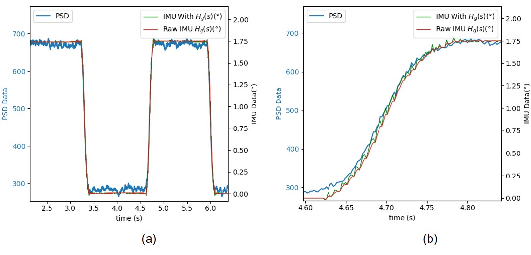
Figure 16: PSD raw data and IMU measurement results without motion compensation. IMU is the original IMU measurements, processed IMU is the IMU results processed with the compensator $H_{g}(s)$. (b) is the zoom-in the result of (a).

Fig. 17 shows the motion compensation results comparison under various motor speed ($t$, motor transient time) and with and without the compensator $H_{g}(s)$. When the motor speed gets faster, the motion compensation errors increase, and $H_{g}(s)$ can effectively reduce the error.

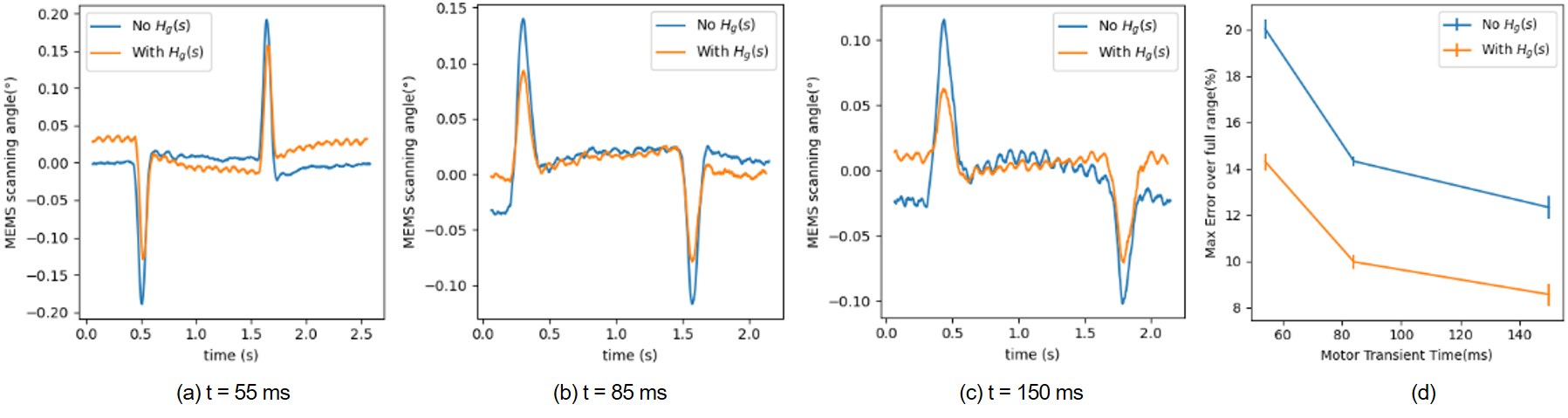
Figure 17: The motion compensation results comparison under different motor speed (t, motor transient time) and with and without the compensator $H_{g}(s)$. When the motor speed gets faster, the motion compensation errors become larger. $H_{g}(s)$ can effectively improve the compensation scanning.

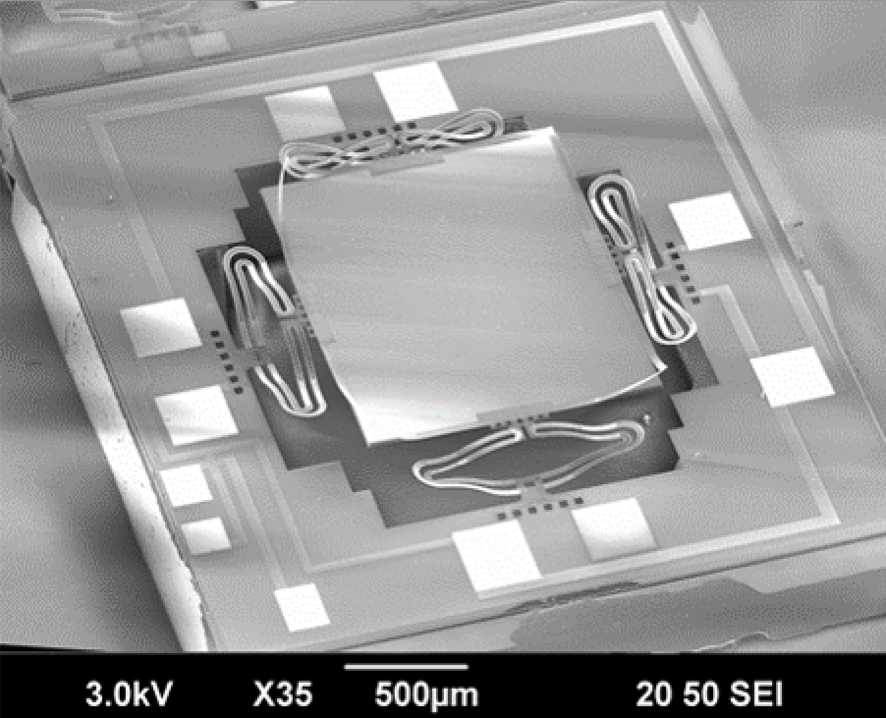
(a)

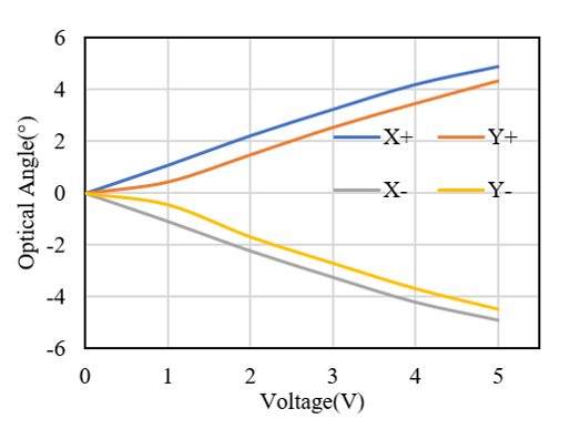
(b)

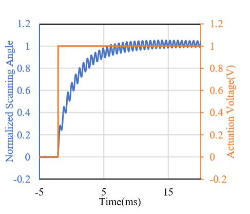
(c)

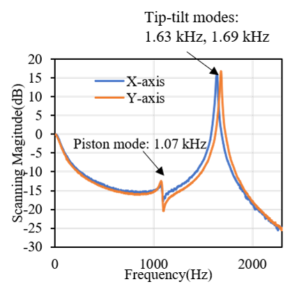
(d)

Figure 18: (a) An SEM image of the fabricated MEMS mirror. (b) The optical scanning angle response of the MEMS mirror. (c) The step response of the MEMS mirror is 5 ms. (d)The frequency response of the MEMS mirror.

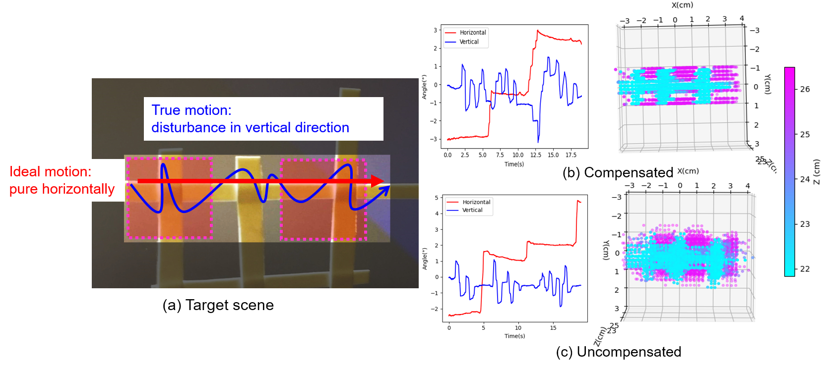
Figure 19: Compensated point cloud stitching and experiment and its results. (a) The target scene placed at 22 cm from the LiDAR. The red line is the ideal motion, the blue line qualitatively depicts the type of experiment we performed, with vertical disturbances only. The graphs show the actual, measured disturbances. (b) With compensated scanning, the recorded motion and the generated point cloud show sharper depth edges than that with (c) with uncompensated scanning.

The motion compensation under continuous sinusoidal drive disturbance is also tested. The motor drives the MEMS mirror scanner head with sinusoidal motions. The MEMS compensated scanning system tries to compensate the scanning angle to an ideal direction. The effect with and without the compensator term is also compared, as shown in Table I.

Table I: A comparison of the errors under step motion disturbance and continuous sinusoidal motion disturbance on a step motion with the $H_{g}(s)$ present or not.

MEMS and Robot Motion Shock

The mirror has a maximum actuation voltage of 5 V and a scanning FoV of $-4.8^{\circ}$ to $+5.2^{\circ}$ in the horizontal axis and $-3.8^{\circ}$ to $+4.3^{\circ}$ in the vertical axis (Fig. 18(b)). The voltage to MEMS tilting angle response is approximately linear. The MEMS mirror can perform non-resonant arbitrary scanning or pointing according to the control signal. The cross-axis sensitivity is about 6 $\%$ in both axes. In the micro-controller, the voltage and the MEMS scanning angle is approximated with a linear relationship with the cross-axis sensitivity taken into considered. The maximum error caused by the non-linearity is $0.3^{\circ}$.

The step response is 5 ms (Fig. 18(c)(a)) with very small ringing. To test the frequency response, the frequency of the actuation voltage is swept and the actual tilt angle is measured by tracking the light beam reflected from the mirror plate using a position sensing detector (PSD), shown in Fig. 18(d)(b). The piston resonant mode is found at $f_{1}$=1.07kHz and the tip-tilting resonant modes are at $f_{2}=$1.63 kHz and $f_{3}=$ 1.69 kHz.

The tip-tilt scanning response of the MEMS mirror is modeled with a 3rd order system according to [27]. The transfer function $H_{1}(s)$ can be expressed as,

$$H_{1}(s)=\frac{\frac{1}{\tau}\omega_{n}^{2}}{(s^{2}+2\omega_{n}\zeta s+\omega_{n}^{2})(s+\frac{1}{\tau})}$$ (22)

where $\tau$ is the thermal time constant, $\tau\approx t_{r}/2.2=2.3ms$; $\omega_{n}$ is the natural resonant frequency of the mirror rotation, $\omega_{n}\approx 2\pi\text{(1.65 kHz)}$, and $\zeta$ is the damping ratio of the bimorph-mirror plate system, $\zeta\approx 1/2Q=0.006$. Thus, the transfer function $H_{1}(s)$ of the MEMS mirror can be obtained by substituting and slightly tuning the parameters in Eq. 22.

Similar to [49], the MEMS mirror is actuated by the PWM signals with a voltage level of 0-5V. The PWM signal can be generated by an Arduino Mega microcontroller at 15 kHz and 8 bit. The ringing of a step response is less than 2 $\%$ after about 10 ms. The minimal achievable step is 0.035^∘ which is much smaller than the linearization error.

We now show expressions for the acceleration and forces generated by a MEMS mirror scan. The small-angle tip-tilt scanning stiffness $k_{\mbox{r}}$ is

$$k_{\text{r}}=I(2\pi f_{r})^{2}$$ (23)

where $f_{r}$ is the resonant frequency of the tip-tilting modes ($f_{2},f_{3}$); $I$ is the moment of inertia of the mirror plate alone its tip-tilting axis,

$$I=\frac{1}{12}m_{\text{plate}}(t^{2}+d^{2})$$ (24)

where $t$ is the thickness of the mirror plate, and $d$ is the length of the mirror plate. The rotation stiffness $k_{\mbox{r}}$ = 2.16e-6 N$\cdot$m/rad. With an external angular acceleration of $\ddot{\theta}$ alone on the mirror rotation axis, the excited mirror rotation $\theta$ is

$$\theta=-\frac{I\ddot{\theta}}{k_{r}}=\text{-1e-8}\cdot\ddot{\theta}.$$ (25)

Take the mirror scanning step $0.25^{\circ}$ as the maximum tolerance of the excited mirror plate rotation, the tolerable external angular acceleration is $\ddot{\theta}$ = 44000 rad/$\text{s}^{2}$. The maximum angular acceleration of a commercialized robot is usually less than 1000 rad/$\text{s}^{2}$, and the excited MEMS mirror rotation is less than 6e-4^∘ which can be ignored. Since this MEMS mirror has four identical actuators and the difference on the two axes alone are small, the excited MEMS mirror rotation under robot vibration can be ignored.

We now consider robot crash scenarios. The MEMS mirror can also survive most of the extreme vibration or mechanical shock without failure. The stiffness of the MEMS mirror under shock $k_{\mbox{p}}$ is:

$$k_{\mbox{p}}=m_{\text{plate}}(2\pi f_{1})^{2}$$ (26)

where $m_{plate}$ is the mass of the mirror plate. Thus, the stiffness the MEMS mirror in piston motion is $k_{p}$ = 3.2 N/m. The maximum allowable piston displacement of the mirror plate without failure is $d_{\mbox{max}}$= 200$\upmu$m. The maximum tolerable acceleration in the direction perpendicular to the mirror plate is $a_{max}$ is

$$a_{max}=\frac{k_{\text{p}}d_{\text{max}}}{m_{\text{plate}}}=5500\text{m}/\text{s}^{2}.$$ (27)

For most commercial robots, maximum tolerable shock is under 1000 $\text{m}/\text{s}^{2}$. So the MEMS mirror can survive most of the mechanical shock and vibration of the robot. External vibration around the resonant frequency will excite large MEMS mirror vibration or even damage the mirror. To avoid the resonance effect, the MEMS mirror should avoid being actuated around the resonant frequency ($f_{1},f_{2},f_{3}$).

Stitching experiments with translation

Here, we performed point-cloud stitching as that sensor moves along an object. The target scanning area is along the horizontal paper-cut figure shown in the highlighted area in the Figure 19 (a). The blue line is an example of the true motion with disturbance only existing in the vertical direction. As the LiDAR rotates from in the horizontal direction from left to right, it is expected to collect the best point cloud covering the highlight area of the object only. The result of compensated scanning and uncompensated scanning are shown in Figures 19 (b) and (c) on the right side, with their measured motions on the left side. Please find other supplementary materials in the accompanying video.

References

- [1] Thiemo Alldieck et al. “Optical flow-based 3d human motion estimation from monocular video” In German Conference on Pattern Recognition, 2017, pp. 347–360 Springer
- [2] Riccardo Antonello et al. “IMU-aided image stabilization and tracking in a HSM-driven camera positioning unit” In 2013 IEEE International Symposium on Industrial Electronics, 2013, pp. 1–7 IEEE
- [3] Moshe Ben-Ezra, Assaf Zomet and Shree K Nayar “Jitter camera: High resolution video from a low resolution detector” In Proceedings of the 2004 IEEE Computer Society Conference on Computer Vision and Pattern Recognition, 2004. CVPR 2004. 2, 2004, pp. II–II IEEE
- [4] Andreas Bircher et al. “Receding horizon” next-best-view” planner for 3d exploration” In 2016 IEEE international conference on robotics and automation (ICRA), 2016, pp. 1462–1468 IEEE
- [5] Andrea Censi “On achievable accuracy for range-finder localization” In Proceedings 2007 IEEE International Conference on Robotics and Automation, 2007, pp. 4170–4175 IEEE
- [6] Chao-Ho Chen, Yi-Li Kuo, Tsong-Yi Chen and Jie-Ru Chen “Real-time video stabilization based on motion compensation” In 2009 Fourth International Conference on Innovative Computing, Information and Control (ICICIC), 2009, pp. 1495–1498 IEEE
- [7] Gabriele Costante et al. “Perception-aware Path Planning” In IEEE Transactions on Robotics Institute of ElectricalElectronics Engineers, 2016, pp. Epub–ahead
- [8] Frank Dellaert “Factor graphs and GTSAM: A hands-on introduction”, 2012
- [9] Xinke Deng et al. “Feature-constrained active visual SLAM for mobile robot navigation” In 2018 IEEE International Conference on Robotics and Automation (ICRA), 2018, pp. 7233–7238 IEEE
- [10] Paul Furgale, Joern Rehder and Roland Siegwart “Unified temporal and spatial calibration for multi-sensor systems” In 2013 IEEE/RSJ International Conference on Intelligent Robots and Systems, 2013, pp. 1280–1286 IEEE
- [11] Andreas Geiger, Philip Lenz and Raquel Urtasun “Are we ready for autonomous driving? the kitti vision benchmark suite” In 2012 IEEE conference on computer vision and pattern recognition, 2012, pp. 3354–3361 IEEE
- [12] Zan Gojcic, Caifa Zhou, Jan D Wegner and Andreas Wieser “The perfect match: 3d point cloud matching with smoothed densities” In Proceedings of the IEEE/CVF Conference on Computer Vision and Pattern Recognition, 2019, pp. 5545–5554
- [13] Heinrich Grüger et al. “3.1: MOEMS Laser Projector for Handheld Devices Featuring Motion Compensation” In SID Symposium Digest of Technical Papers 38.1, 2007, pp. 1–3 Wiley Online Library
- [14] Richard Hartley, Jochen Trumpf, Yuchao Dai and Hongdong Li “Rotation averaging” In International journal of computer vision 103.3 Springer, 2013, pp. 267–305
- [15] “Hawk Head Stabilization” In YouTube YouTube, 2020 URL: https://www.youtube.com/watch?v=aqgewVCC0k0
- [16] Tomohiko Hayakawa, Takanoshin Watanabe, Taku Senoo and Masatoshi Ishikawa “Gain-compensated sinusoidal scanning of a galvanometer mirror in proportional-integral-differential control using the pre-emphasis technique for motion-blur compensation” In Applied Optics 55.21 Optical Society of America, 2016, pp. 5640–5646
- [17] E Farrell Helbling, Sawyer B Fuller and Robert J Wood “Pitch and yaw control of a robotic insect using an onboard magnetometer” In 2014 IEEE international conference on robotics and automation (ICRA), 2014, pp. 5516–5522 IEEE
- [18] Katie Lynn Hoffman “Design and locomotion studies of a miniature centipede-inspired robot”, 2013
- [19] Stefan Hrabar, Peter Corke and Volker Hilsenstein “PTZ camera pose estimation by tracking a 3D target” In 2011 IEEE International Conference on Robotics and Automation, 2011, pp. 240–247 IEEE
- [20] Kota Ito et al. “System Design and Performance Characterization of a MEMS-Based Laser Scanning Time-of-Flight Sensor Based on a 25664-pixel Single-Photon Imager” In IEEE Photonics Journal 5.2 IEEE, 2013, pp. 6800114–6800114
- [21] Kemiao Jia, Sagnik Pal and Huikai Xie “An electrothermal tip–tilt–piston micromirror based on folded dual S-shaped bimorphs” In Journal of Microelectromechanical systems 18.5 IEEE, 2009, pp. 1004–1015
- [22] Ruting Jia et al. “System performance of an inertially stabilized gimbal platform with friction, resonance, and vibration effects” In Journal of Nonlinear Dynamics 2017 Hindawi, 2017
- [23] Abhishek Kasturi, Veljko Milanovic, Bryan H Atwood and James Yang “UAV-borne lidar with MEMS mirror-based scanning capability” In Laser Radar Technology and Applications XXI 9832, 2016, pp. 98320M International Society for OpticsPhotonics
- [24] Katsumi Kimoto et al. “Development of small size 3D LIDAR” In 2014 IEEE International Conference on Robotics and Automation (ICRA), 2014, pp. 4620–4626 IEEE
- [25] Rainer Kümmerle et al. “g 2 o: A general framework for graph optimization” In 2011 IEEE International Conference on Robotics and Automation, 2011, pp. 3607–3613 IEEE
- [26] GEN LI, Jae Kyu Suhr, Seung-In Noh and Jaihie Kim “Tracking moving objects by using a pan-tilt-zoom camera” In ITC-CSCC: International Technical Conference on Circuits Systems, Computers and Communications, 2009, pp. 1012–1015
- [27] Mengyuan Li et al. “Modelling and experimental verification of step response overshoot removal in electrothermally-actuated mems mirrors” In Micromachines 8.10 Multidisciplinary Digital Publishing Institute, 2017, pp. 289
- [28] Quanchao Li et al. “Nonorthogonal Aerial Optoelectronic Platform Based on Triaxial and Control Method Designed for Image Sensors” In Sensors 20.1 Multidisciplinary Digital Publishing Institute, 2020, pp. 10
- [29] Ievgeniia Maksymova, Philipp Greiner, Leonhard Christian Niedermueller and Norbert Druml “Detection and Compensation of Periodic Jitters of Oscillating MEMS Mirrors used in Automotive Driving Assistance Systems” In 2019 IEEE Sensors Applications Symposium (SAS), 2019, pp. 1–5 IEEE
- [30] Veljko Milanović, Abhishek Kasturi, James Yang and Frank Hu “Closed-loop control of gimbal-less MEMS mirrors for increased bandwidth in LiDAR applications” In Laser Radar Technology and Applications XXII 10191, 2017, pp. 101910N International Society for OpticsPhotonics
- [31] Yash Mulgaonkar, Gareth Cross and Vijay Kumar “Design of small, safe and robust quadrotor swarms” In 2015 IEEE international conference on robotics and automation (ICRA), 2015, pp. 2208–2215 IEEE
- [32] Frank Neuhaus, Tilman Koß, Robert Kohnen and Dietrich Paulus “Mc2slam: Real-time inertial lidar odometry using two-scan motion compensation” In German Conference on Pattern Recognition, 2018, pp. 60–72 Springer
- [33] Yue Pan et al. “MULLS: Versatile LiDAR SLAM via multi-metric linear least square” In 2021 IEEE International Conference on Robotics and Automation (ICRA), 2021, pp. 11633–11640 IEEE
- [34] Tao Peng and Satyandra K Gupta “Model and algorithms for point cloud construction using digital projection patterns”, 2007
- [35] Ethan Phelps and Charles A Primmerman “Blind Compensation of Angle Jitter for Satellite-Based Ground-Imaging Lidar” In IEEE Transactions on Geoscience and Remote Sensing 58.2 IEEE, 2019, pp. 1436–1449
- [36] Seyed Abbas Sadat et al. “Feature-rich path planning for robust navigation of MAVs with mono-SLAM” In 2014 IEEE International Conference on Robotics and Automation (ICRA), 2014, pp. 3870–3875 IEEE
- [37] Artur Sagitov and Yuri Gerasimov “Towards DJI phantom 4 realistic simulation with gimbal and RC controller in ROS/Gazebo environment” In 2017 10th International Conference on Developments in eSystems Engineering (DeSE), 2017, pp. 262–266 IEEE
- [38] Shital Shah, Debadeepta Dey, Chris Lovett and Ashish Kapoor “Airsim: High-fidelity visual and physical simulation for autonomous vehicles” In Field and service robotics, 2018, pp. 621–635 Springer
- [39] Tixiao Shan et al. “Lio-sam: Tightly-coupled lidar inertial odometry via smoothing and mapping” In 2020 IEEE/RSJ international conference on intelligent robots and systems (IROS), 2020, pp. 5135–5142 IEEE
- [40] Jae Kyu Suhr et al. “Background compensation for pan-tilt-zoom cameras using 1-D feature matching and outlier rejection” In IEEE transactions on circuits and systems for video technology 21.3 IEEE, 2010, pp. 371–377
- [41] Takafumi Taketomi and Janne Heikkila “Focal length change compensation for monocular slam” In 2015 IEEE International Conference on Image Processing (ICIP), 2015, pp. 4982–4986 IEEE
- [42] Takafumi Taketomi and Janne Heikkilä “Zoom factor compensation for monocular SLAM” In 2015 IEEE Virtual Reality (VR), 2015, pp. 293–294 IEEE
- [43] Takafumi Taketomi, Hideaki Uchiyama and Sei Ikeda “Visual SLAM algorithms: a survey from 2010 to 2016” In IPSJ Transactions on Computer Vision and Applications 9.1 Springer, 2017, pp. 16
- [44] Zaid Tasneem et al. “Adaptive fovea for scanning depth sensors” In The International Journal of Robotics Research 39.7 SAGE Publications Sage UK: London, England, 2020, pp. 837–855
- [45] Sebastian Thrun “Probabilistic robotics” In Communications of the ACM 45.3 ACM New York, NY, USA, 2002, pp. 52–57
- [46] Robert K Tyson “Performance assessment of MEMS adaptive optics in tactical airborne systems” In Adaptive Optics Systems and Technology 3762, 1999, pp. 91–100 International Society for OpticsPhotonics
- [47] Dingkang Wang, Connor Watkins and Huikai Xie “MEMS Mirrors for LiDAR: A review” In Micromachines 11.5 Multidisciplinary Digital Publishing Institute, 2020, pp. 456
- [48] Dingkang Wang et al. “A Large Aperture 2-Axis Electrothermal MEMS Mirror for Compact 3D LiDAR” In 2019 International Conference on Optical MEMS and Nanophotonics (OMN), 2019, pp. 180–181 IEEE
- [49] Dingkang Wang et al. “A low-voltage, low-current, digital-driven MEMS mirror for low-power LiDAR” In IEEE Sensors Letters 4.8 IEEE, 2020, pp. 1–4
- [50] Dingkang Wang et al. “An ultra-fast electrothermal micromirror with bimorph actuators made of copper/tungsten” In 2017 International Conference on Optical MEMS and Nanophotonics (OMN), 2017, pp. 1–2 IEEE
- [51] Robert Wood, Radhika Nagpal and Gu-Yeon Wei “flight of the robobees” In Scientific American 308.3 Scientific American, a division of Nature America, Inc., 2013, pp. 60–65 URL: http://www.jstor.org/stable/26018027
- [52] Wei Xu et al. “Fast-lio2: Fast direct lidar-inertial odometry” In IEEE Transactions on Robotics IEEE, 2022
- [53] Dong Xue et al. “Computational simulation and free flight validation of body vibration of flapping-wing MAV in forward flight” In Aerospace Science and Technology 95 Elsevier, 2019, pp. 105491
- [54] Guang-Zhong Yang et al. “The grand challenges of Science Robotics” In Science robotics 3.14 AAAS, 2018, pp. eaar7650
- [55] Heng Yang, Jingnan Shi and Luca Carlone “Teaser: Fast and certifiable point cloud registration” In IEEE Transactions on Robotics 37.2 IEEE, 2020, pp. 314–333
- [56] Haoyang Ye, Yuying Chen and Ming Liu “Tightly coupled 3d lidar inertial odometry and mapping” In 2019 International Conference on Robotics and Automation (ICRA), 2019, pp. 3144–3150 IEEE
- [57] Ji Zhang and Sanjiv Singh “LOAM: Lidar Odometry and Mapping in Real-time.” In Robotics: Science and Systems 2.9, 2014
- [58] Xiaoyang Zhang, Liang Zhou and Huikai Xie “A fast, large-stroke electrothermal MEMS mirror based on Cu/W bimorph” In Micromachines 6.12 Multidisciplinary Digital Publishing Institute, 2015, pp. 1876–1889
- [59] Zichao Zhang and Davide Scaramuzza “Beyond point clouds: Fisher information field for active visual localization” In 2019 International Conference on Robotics and Automation (ICRA), 2019, pp. 5986–5992 IEEE
- [60] Zichao Zhang and Davide Scaramuzza “Perception-aware receding horizon navigation for MAVs” In 2018 IEEE International Conference on Robotics and Automation (ICRA), 2018, pp. 2534–2541 IEEE