$(\alpha_{D},\alpha_{G})$-GANs: Addressing GAN Training Instabilities via Dual Objectives

Abstract

In an effort to address the training instabilities of GANs, we introduce a class of dual-objective GANs with different value functions (objectives) for the generator (G) and discriminator (D). In particular, we model each objective using $\alpha$-loss, a tunable classification loss, to obtain $(\alpha_{D},\alpha_{G})$-GANs, parameterized by $(\alpha_{D},\alpha_{G})\in(0,\infty]^{2}$. For sufficiently large number of samples and capacities for G and D, we show that the resulting non-zero sum game simplifies to minimizing an $f$-divergence under appropriate conditions on $(\alpha_{D},\alpha_{G})$. In the finite sample and capacity setting, we define estimation error to quantify the gap in the generator’s performance relative to the optimal setting with infinite samples and obtain upper bounds on this error, showing it to be order optimal under certain conditions. Finally, we highlight the value of tuning $(\alpha_{D},\alpha_{G})$ in alleviating training instabilities for the synthetic 2D Gaussian mixture ring and the Stacked MNIST datasets.

I Introduction

Generative adversarial networks (GANs) have become a crucial data-driven tool for generating synthetic data. GANs are generative models trained to produce samples from an unknown (real) distribution using a finite number of training data samples. They consist of two modules, a generator G and a discriminator D, parameterized by vectors $\theta\in\Theta\subset\mathbb{R}^{n_{g}}$ and $\omega\in\Omega\subset\mathbb{R}^{n_{d}}$, respectively, which play an adversarial game with each other. The generator $G_{\theta}$ maps noise $Z\sim P_{Z}$ to a data sample in $\mathcal{X}$ via the mapping $z\mapsto G_{\theta}(z)$ and aims to mimic data from the real distribution $P_{r}$. The discriminator $D_{\omega}$ takes as input $x\in\mathcal{X}$ and classifies it as real or generated by computing a score $D_{\omega}(x)\in[0,1]$ which reflects the probability that $x$ comes from $P_{r}$ (real) as opposed to $P_{G_{\theta}}$ (synthetic). For a chosen value function $V(\theta,\omega)$, the adversarial game between G and D can be formulated as a zero-sum min-max problem given by

$$\inf_{\theta\in\Theta}\sup_{\omega\in\Omega}\,V(\theta,\omega).$$ (1)

Goodfellow et al. [1] introduce the vanilla GAN for which

$$V_{\text{VG}}(\theta,\omega)=\mathbb{E}_{X\sim P_{r}}[\log{D_{\omega}(X)}]+\mathbb{E}_{X\sim P_{G_{\theta}}}[\log{(1-D_{\omega}(X))}].$$

For this $V_{\text{VG}}$, they show that when the discriminator class $\{D_{\omega}\}_{\omega\in\Omega}$ is rich enough, (1) simplifies to minimizing the Jensen-Shannon divergence [2] between $P_{r}$ and $P_{G_{\theta}}$.

Various other GANs have been studied in the literature using different value functions, including $f$-divergence based GANs called $f$-GANs [3], IPM based GANs [4, 5, 6], etc. Observing that the discriminator is a classifier, recently, Kurri et al. [7, 8] show that the value function in (1) can be written using a class probability estimation (CPE) loss $\ell(y,\hat{y})$ whose inputs are the true label $y\in\{0,1\}$ and predictor $\hat{y}\in[0,1]$ (soft prediction of $y$) as

$$V(\theta,\omega)=\mathbb{E}_{X\sim P_{r}}[-\ell(1,D_{\omega}(X))]+\mathbb{E}_{X\sim P_{G_{\theta}}}[-\ell(0,D_{\omega}(X))].$$

Using this approach, they introduce $\alpha$-GAN using the tunable CPE loss $\alpha$-loss [9, 10], defined for $\alpha\in(0,\infty]$ as

$$\ell_{\alpha}(y,\hat{y})\coloneqq\frac{\alpha}{\alpha-1}\left(1-y\hat{y}^{\frac{\alpha-1}{\alpha}}-(1-y)(1-\hat{y})^{\frac{\alpha-1}{\alpha}}\right).$$ (2)

They show that the $\alpha$-GAN formulation recovers various $f$-divergence based GANs including the Hellinger GAN [3] ($\alpha=1/2$), the vanilla GAN [1] ($\alpha=1$), and the Total Variation (TV) GAN [3] ($\alpha=\infty$). Further, for a large enough discriminator class, the min-max optimization for $\alpha$-GAN in (1) simplifies to minimizing the Arimoto divergence [11, 12].

While each of the abovementioned GANs have distinct advantages, they continue to suffer from one or more types of training instabilities, including vanishing/exploding gradients, mode collapse, and sensitivity to hyperparameter tuning. In [1], Goodfellow et al. note that the generator’s objective in the vanilla GAN can saturate early in training (due to the use of the sigmoid activation) when D can easily distinguish between the real and synthetic samples, i.e., when the output of D is near zero for all synthetic samples, leading to vanishing gradients. Further, a confident D induces a steep gradient at samples close to the real data, thereby preventing G from learning such samples due to exploding gradients. To alleviate these, [1] proposes a non-saturating (NS) generator objective:

$$V_{\text{VG}}^{\text{NS}}(\theta,\omega)=\mathbb{E}_{X\sim P_{G_{\theta}}}[-\log{D_{\omega}(X)}].$$ (3)

This NS version of the vanilla GAN may be viewed as involving different objective functions for the two players (in fact, with two versions of the $\alpha=1$ CPE loss, i.e., log-loss, for D and G). However, it continues to suffer from mode collapse [13, 14]. While other dual-objective GANs have also been proposed (e.g., Least Squares GAN (LSGAN) [15], RényiGAN [16], NS $f$-GAN [3], hybrid $f$-GAN [17]), few have had success fully addressing training instabilities.

Recent results have shown that $\alpha$-loss demonstrates desirable gradient behaviors for different $\alpha$ values [10]. It also assures learning robust classifiers that can reduce the confidence of D (a classifier) thereby allowing G to learn without gradient issues. To this end, we introduce a different $\alpha$-loss objective for each player to address training instabilities. We propose a tunable dual-objective $(\alpha_{D},\alpha_{G})$-GAN, where the objective functions of D and G are written in terms of $\alpha$-loss with parameters $\alpha_{D}\in(0,\infty]$ and $\alpha_{G}\in(0,\infty]$, respectively. Our key contributions are:

• For this non-zero sum game, we show that a Nash equilibrium exists. For appropriate $(\alpha_{D},\alpha_{G})$ values, we derive the optimal strategies for D and G and prove that for the optimal $D_{\omega^{*}}$, G minimizes an $f$-divergence and can therefore learn the real distribution $P_{r}$.

• Since $\alpha$-GAN captures various GANs, including the vanilla GAN, it can potentially suffer from vanishing gradients due to a saturation effect. We address this by introducing a non-saturating version of the $(\alpha_{D},\alpha_{G})$-GAN and present its Nash equilibrium strategies for D and G.

• A natural question that arises is how to quantify the theoretical guarantees for dual-objective GANs, specifically for $(\alpha_{D},\alpha_{G})$-GANs, in terms of their estimation capabilities in the setting of limited capacity models and finite training samples. To this end, we define estimation error for $(\alpha_{D},\alpha_{G})$-GANs, present an upper bound on the error, and a matching lower bound under additional assumptions.

• Finally, we demonstrate empirically that tuning $\alpha_{D}$ and $\alpha_{G}$ significantly reduces vanishing and exploding gradients and alleviates mode collapse on a synthetic 2D-ring dataset. For the high-dimensional Stacked MNIST dataset, we show that our tunable approach is more robust in terms of mode coverage to the choice of GAN hyperparameters, including number of training epochs and learning rate, relative to both vanilla GAN and LSGAN.

II Main Results

II-A $(\alpha_{D},\alpha_{G})$-GAN

We first propose a dual-objective $(\alpha_{D},\alpha_{G})$-GAN with different objective functions for the generator and discriminator. In particular, the discriminator maximizes $V_{\alpha_{D}}(\theta,\omega)$ while the generator minimizes $V_{\alpha_{G}}(\theta,\omega)$, where

$$V_{\alpha}(\theta,\omega)$$

$$=\mathbb{E}_{X\sim P_{r}}[-\ell_{\alpha}(1,D_{\omega}(X))]+\mathbb{E}_{X\sim P_{G_{\theta}}}[-\ell_{\alpha}(0,D_{\omega}(X))],$$ (4)

for $\alpha=\alpha_{D},\alpha_{G}\in(0,\infty]$. We recover the $\alpha$-GAN [7, 8] value function when $\alpha_{D}=\alpha_{G}=\alpha$. The resulting $(\alpha_{D},\alpha_{G})$-GAN is given by

$$\sup_{\omega\in\Omega}V_{\alpha_{D}}(\theta,\omega)$$ (5a)

$$\inf_{\theta\in\Theta}V_{\alpha_{G}}(\theta,\omega).$$ (5b)

The following theorem presents the conditions under which the optimal generator learns the real distribution $P_{r}$ when the discriminator set $\Omega$ is large enough.

Theorem 1.

For a fixed generator $G_{\theta}$, the discriminator optimizing (5a) is given by

$$D_{\omega^{*}}(x)=\frac{p_{r}(x)^{\alpha_{D}}}{p_{r}(x)^{\alpha_{D}}+p_{G_{\theta}}(x)^{\alpha_{D}}},$$ (6)

where $p_{r}$ and $p_{G_{\theta}}$ are the corresponding densities of the distributions $P_{r}$ and $P_{G_{\theta}}$, respectively, with respect to a base measure $dx$ (e.g., Lebesgue measure). For this $D_{\omega^{*}}$ and the function $f_{\alpha_{D},\alpha_{G}}:\mathbb{R}_{+}\to\mathbb{R}$ defined as

$$f_{\alpha_{D},\alpha_{G}}(u)=\frac{\alpha_{G}}{\alpha_{G}-1}\left(\frac{u^{\alpha_{D}\left(1-\frac{1}{\alpha_{G}}\right)+1}+1}{(u^{\alpha_{D}}+1)^{1-\frac{1}{\alpha_{G}}}}-2^{\frac{1}{\alpha_{G}}}\right),$$ (7)

(5b) simplifies to minimizing a non-negative symmetric $f_{\alpha_{D},\alpha_{G}}$-divergence $D_{f_{\alpha_{D},\alpha_{G}}}(\cdot||\cdot)$ as

$$\inf_{\theta\in\Theta}D_{f_{\alpha_{D},\alpha_{G}}}(P_{r}||P_{G_{\theta}})+\frac{\alpha_{G}}{\alpha_{G}-1}\left(2^{\frac{1}{\alpha_{G}}}-2\right),$$ (8)

which is minimized iff $P_{G_{\theta}}=P_{r}$ for $(\alpha_{D},\alpha_{G})\in(0,\infty]^{2}$ such that $\Big{(}\alpha_{D}\leq 1,\;\alpha_{G}>\frac{\alpha_{D}}{\alpha_{D}+1}\Big{)}\;\text{ or }\;\Big{(}\alpha_{D}>1,\;\frac{\alpha_{D}}{2}<\alpha_{G}\leq\alpha_{D}\Big{)}$.

Proof.

We substitute the optimal discriminator of (5a) into the objective function of (5b) and translate it into the form

$$\int_{\mathcal{X}}p_{G_{\theta}}(x)f_{\alpha_{D},\alpha_{G}}\left(\frac{p_{r}(x)}{p_{G_{\theta}}(x)}\right)dx+\frac{\alpha_{G}}{\alpha_{G}-1}\left(2^{\frac{1}{\alpha_{G}}}-2\right).$$ (9)

We then find the conditions on $\alpha_{D}$ and $\alpha_{G}$ for $f_{\alpha_{D},\alpha_{G}}$ to be strictly convex so that the first term in (9) is an $f$-divergence. Figure 1(a) illustrates the feasible $(\alpha_{D},\alpha_{G})$-region. A detailed proof can be found in Appendix A. ∎

Noting that $\alpha$-GAN recovers various well-known GANs, including the vanilla GAN, which is prone to saturation, the $(\alpha_{D},\alpha_{G})$-GAN formulation using the generator objective function in (4) can similarly saturate early in training, causing vanishing gradients. We therefore propose the following NS alternative to the generator’s objective in (4):

$$V^{\text{NS}}_{\alpha_{G}}(\theta,\omega) =\mathbb{E}_{X\sim P_{G_{\theta}}}[\ell_{\alpha_{G}}(1,D_{\omega}(X))],$$ (10)

thereby replacing (5b) with

$$\inf_{\theta\in\Theta}V^{\text{NS}}_{\alpha_{G}}(\theta,\omega).$$ (11)

Comparing (5b) and (11), note that the additional expectation term over $P_{r}$ in (4) results in (5b) simplifying to a symmetric divergence for $D_{\omega^{*}}$ in (6), whereas the single term in (10) will result in (11) simplifying to an asymmetric divergence. The optimal discriminator for this NS game remains the same as in (6). The following theorem provides the solution to (11) under the assumption that the optimal discriminator can be attained.

Theorem 2.

For the same $D_{\omega^{*}}$ in (6) and the function $f_{\alpha_{D},\alpha_{G}}^{\text{NS}}:\mathbb{R}_{+}\to\mathbb{R}$ defined as

$$f^{\text{NS}}_{\alpha_{D},\alpha_{G}}(u)=\frac{\alpha_{G}}{\alpha_{G}-1}\left(2^{\frac{1}{\alpha_{G}}-1}-\frac{u^{\alpha_{D}\left(1-\frac{1}{\alpha_{G}}\right)}}{(u^{\alpha_{D}}+1)^{1-\frac{1}{\alpha_{G}}}}\right),$$ (12)

(5b) simplifies to minimizing a non-negative asymmetric $f^{\text{NS}}_{\alpha_{D},\alpha_{G}}$-divergence $D_{f^{\text{NS}}_{\alpha_{D},\alpha_{G}}}(\cdot||\cdot)$ as

$$\inf_{\theta\in\Theta}D_{f^{\text{NS}}_{\alpha_{D},\alpha_{G}}}(P_{r}||P_{G_{\theta}})+\frac{\alpha_{G}}{\alpha_{G}-1}\left(1-2^{\frac{1}{\alpha_{G}}-1}\right),$$ (13)

which is minimized iff $P_{G_{\theta}}=P_{r}$ for $(\alpha_{D},\alpha_{G})\in(0,\infty]^{2}$ such that $\alpha_{D}+\alpha_{G}>\alpha_{G}\alpha_{D}.$

The proof mimics that of Theorem 1 and is detailed in Appendix B. Figure 1(b) illustrates the feasible $(\alpha_{D},\alpha_{G})$-region; in contrast to the saturating setting of Theorem 1, the NS setting constrains $\alpha\leq 2$ when $\alpha_{D}=\alpha_{G}=\alpha$. Nonetheless, we later show empirically in Section III-B that even tuning over this restricted set provides robustness against hyperparameter choices.

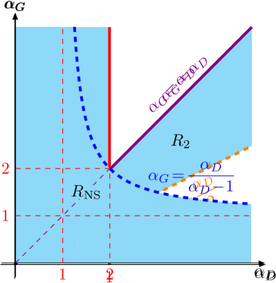
(a)	(b)

Figure 1: (a) Plot of regions $R_{1}=\{(\alpha_{D},\alpha_{G})\in(0,\infty]^{2}\bigm{|}\alpha_{D}\leq 1,\alpha_{G}>\frac{\alpha_{D}}{\alpha_{D}+1}\}$ and $R_{2}=\{(\alpha_{D},\alpha_{G})\in(0,\infty]^{2}\bigm{|}\alpha_{D}>1,\frac{\alpha_{D}}{2}<\alpha_{G}\leq\alpha_{D}\}$ for which $f_{\alpha_{D},\alpha_{G}}$ is strictly convex. (b) Plot of region $R_{\text{NS}}=\{(\alpha_{D},\alpha_{G})\in(0,\infty]^{2}\mid\alpha_{D}+\alpha_{G}>\alpha_{D}\alpha_{G}\}$ for which $f^{\text{NS}}_{\alpha_{D},\alpha_{G}}$ is strictly convex.

II-B Estimation Error

Theorems 1 and 2 assume sufficiently large number of training samples and ample discriminator and generator capacity. However, in practice both the number of training samples and model capacity are usually limited. We consider a setting similar to prior works on generalization and estimation error for GANs (e.g., [18, 8]) with finite training samples $S_{x}=\{X_{1},\dots,X_{n}\}$ and $S_{z}=\{Z_{1},\dots,Z_{m}\}$ from $P_{r}$ and $P_{Z}$, respectively, and with neural networks chosen as the discriminator and generator models. The sets of samples $S_{x}$ and $S_{z}$ induce the empirical real and generated distributions $\hat{P}_{r}$ and $\hat{P}_{G_{\theta}}$, respectively. A useful quantity to evaluate the performance of GANs in this setting is that of the estimation error, defined in [18] as the performance gap of the optimized value function when trained using only finite samples relative to the optimal when the statistics are known. Using this definition, [8] derived upper bounds on this error for $\alpha$-GANs. However, such a definition requires a common value function for both discriminator and generator, and therefore, does not directly apply to the dual-objective setting we consider here.

Our definition relies on the observation that estimation error inherently captures the effectiveness of the generator (for a corresponding optimal discriminator model) in learning with limited samples. We formalize this intuition below.

Since $(\alpha_{D},\alpha_{G})$-GANs use different objective functions for the discriminator and generator, we start by defining the optimal discriminator ${\omega}^{*}$ for a generator model $G_{\theta}$ as

$${\omega}^{*}(P_{r},P_{G_{\theta}})\coloneqq\operatorname*{arg\,max}_{\omega\in\Omega}\;V_{\alpha_{D}}(\theta,\omega)\big{\rvert}_{P_{r},P_{G_{\theta}}},$$ (14)

where the notation $|_{\cdot,\cdot}$ allows us to make explicit the distributions used in the value function. In keeping with the literature where the value function being minimized is referred to as the neural net (NN) distance (since D and G are modeled as neural networks) [19, 18, 8], we define the generator’s NN distance $d_{\omega^{*}(P_{r},P_{G_{\theta}})}$ as

$$d_{\omega^{*}(P_{r},P_{G_{\theta}})}(P_{r},{P}_{G_{{\theta}}})\coloneqq V_{\alpha_{G}}(\theta,\omega^{*}(P_{r},P_{G_{\theta}}))\big{\rvert}_{P_{r},P_{G_{\theta}}}.$$ (15)

The resulting minimization for training the $(\alpha_{D},\alpha_{G})$-GAN using finite samples is

$$\inf_{\theta\in\Theta}d_{\omega^{*}(\hat{P}_{r},\hat{P}_{G_{\theta}})}(\hat{P}_{r},\hat{P}_{G_{{\theta}}}).$$ (16)

Denoting $\hat{\theta}^{*}$ as the minimizer of (16), we define the estimation error for $(\alpha_{D},\alpha_{G})$-GANs as

$$d_{\omega^{*}(P_{r},P_{G_{\hat{\theta}^{*}}})}(P_{r},{P}_{G_{\hat{\theta}^{*}}})-\inf_{\theta\in\Theta}d_{\omega^{*}({P}_{r},{P}_{G_{\theta}})}(P_{r},P_{G_{\theta}}).$$ (17)

We use the same notation as in [8], detailed in the following for easy reference. For $x\in\mathcal{X}\coloneqq\{x\in\mathbb{R}^{d}:||x||_{2}\leq B_{x}\}$ and $z\in\mathcal{Z}\coloneqq\{z\in\mathbb{R}^{p}:||z||_{2}\leq B_{z}\}$, we model the discriminator and generator as $k$- and $l$-layer neural networks, respectively, with

$$D_{\omega} :x\mapsto\sigma\left(\mathbf{w}_{k}^{\mathsf{T}}r_{k-1}(\mathbf{W}_{d-1}r_{k-2}(\dots r_{1}(\mathbf{W}_{1}(x)))\right)\,$$ (18)

$$G_{\theta} :z\mapsto\mathbf{V}_{l}s_{l-1}(\mathbf{V}_{l-1}s_{l-2}(\dots s_{1}(\mathbf{V}_{1}z))),$$ (19)

where (i) $\mathbf{w}_{k}$ is a parameter vector of the output layer; (ii) for $i\in[1:k-1]$ and $j\in[1:l]$, $\mathbf{W}_{i}$ and $\mathbf{V}_{j}$ are parameter matrices; (iii) $r_{i}(\cdot)$ and $s_{j}(\cdot)$ are entry-wise activation functions of layers $i$ and $j$, respectively, i.e., for $\mathbf{a}\in\mathbb{R}^{t}$, $r_{i}(\mathbf{a})=\left[r_{i}(a_{1}),\dots,r_{i}(a_{t})\right]$ and $s_{i}(\mathbf{a})=\left[s_{i}(a_{1}),\dots,s_{i}(a_{t})\right]$; and (iv) $\sigma(\cdot)$ is the sigmoid function given by $\sigma(p)=1/(1+\mathrm{e}^{-p})$. We assume that each $r_{i}(\cdot)$ and $s_{j}(\cdot)$ are $R_{i}$- and $S_{j}$-Lipschitz, respectively, and also that they are positive homogeneous, i.e., $r_{i}(\lambda p)=\lambda r_{i}(p)$ and $s_{j}(\lambda p)=\lambda s_{j}(p)$, for any $\lambda\geq 0$ and $p\in\mathbb{R}$. Finally, as is common in such analysis [20, 21, 22, 18], we assume that the Frobenius norms of the parameter matrices are bounded, i.e., $||\mathbf{W}_{i}||_{F}\leq M_{i}$, $i\in[1:k-1]$, $||\mathbf{w}_{k}||_{2}\leq M_{k}$, and $||\mathbf{V}_{j}||_{F}\leq N_{j}$, $j\in[1:l]$. We now present an upper bound on (17) in the following theorem.

Theorem 3.

In the setting described above, with probability at least $1-2\delta$ over the randomness of training samples $S_{x}=\{X_{i}\}_{i=1}^{n}$ and $S_{z}=\{Z_{j}\}_{j=1}^{m}$, we have

$$d_{\omega^{*}(P_{r},P_{G_{\hat{\theta}^{*}}})}(P_{r},{P}_{G_{\hat{\theta}^{*}}})-\inf_{\theta\in\Theta}d_{\omega^{*}({P}_{r},{P}_{G_{\theta}})}(P_{r},P_{G_{\theta}})$$

$$\leq\frac{4C_{Q_{x}}(\alpha_{G})B_{x}U_{\omega}\sqrt{3k}}{\sqrt{n}}+\frac{4C_{Q_{z}}(\alpha_{G})U_{\omega}U_{\theta}B_{z}\sqrt{3(k+l-1)}}{\sqrt{m}}$$

$$\hskip 12.0pt+U_{\omega}\sqrt{\log{\frac{1}{\delta}}}\left(\frac{4C_{Q_{x}}(\alpha_{G})B_{x}}{\sqrt{2n}}+\frac{4C_{Q_{z}}(\alpha_{G})B_{z}U_{\theta}}{\sqrt{2m}}\right),$$ (20)

where the parameters $U_{\omega}\coloneqq M_{k}\prod_{i=1}^{k-1}(M_{i}R_{i})$ and $U_{\theta}\coloneqq N_{l}\prod_{j=1}^{l-1}(N_{j}S_{j})$, $Q_{x}\coloneqq U_{\omega}B_{x}$, $Q_{z}\coloneqq U_{\omega}U_{\theta}B_{z}$, and

$$C_{h}(\alpha)\coloneqq\begin{cases}\sigma(h)\sigma(-h)^{\frac{\alpha-1}{\alpha}},\ &\alpha\in(0,1]\\ \left(\frac{\alpha-1}{2\alpha-1}\right)^{\frac{\alpha-1}{\alpha}}\frac{\alpha}{2\alpha-1},&\alpha\in(1,\infty).\end{cases}$$ (21)

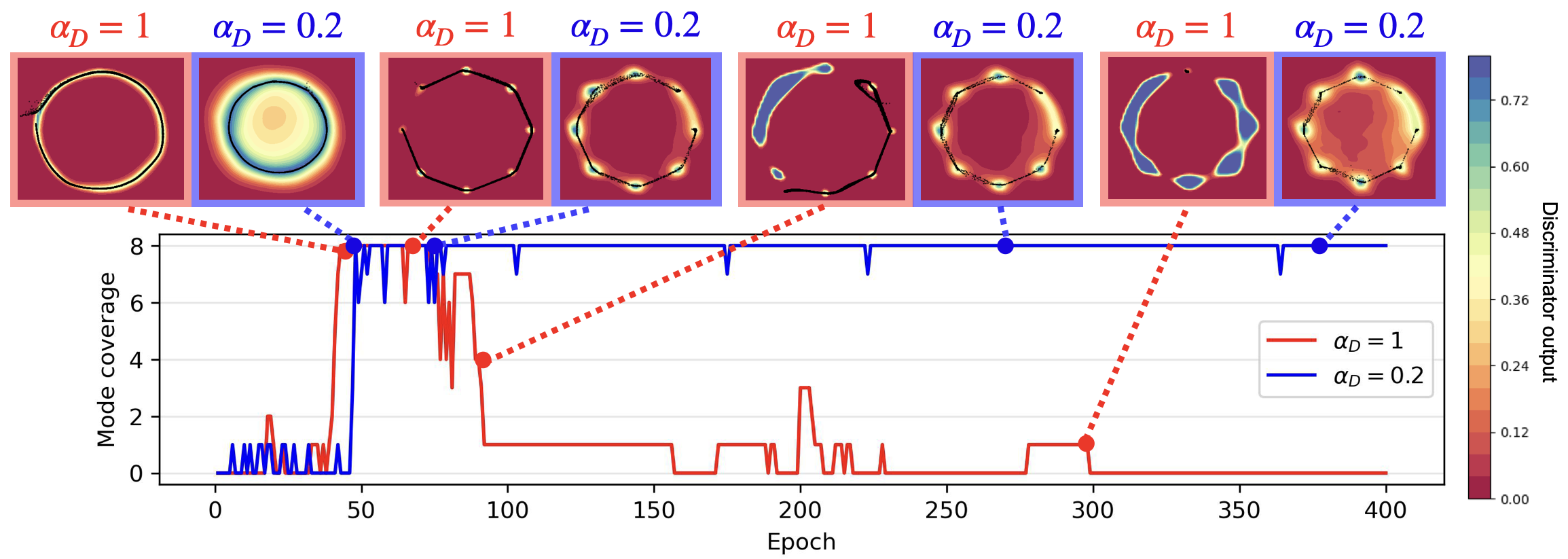
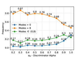
(a)	(b)

Figure 2: (a) Plot of mode coverage over epochs for $(\alpha_{D},\alpha_{G})$-GAN training with the saturating objectives in (5). Fixing $\alpha_{G}=1$, we compare $\alpha_{D}=1$ (vanilla GAN) with $\alpha_{D}=0.2$. Placed above this plot are 2D visuals of the generated samples (in black) at different epochs; these show that both GANs successfully capture the ring-like structure, but the vanilla GAN fails to maintain the ring over time. We illustrate the discriminator output in the same visual as a heat map to show that the $\alpha_{D}=1$ discriminator exhibits more confident predictions (tending to 0 or 1), which in turn subjects G to vanishing and exploding gradients when its objective $\log(1-D)$ saturates as $D\rightarrow 0$ and diverges as $D\rightarrow 1$, respectively. This combination tends to repel the generated data when it approaches the real data, thus freezing any significant weight update in the future. In contrast, the less confident predictions of the $(0.2,1)$-GAN create a smooth landscape for the generated output to descend towards the real data. (b) Plot of success and failure rates over 200 seeds for a range of $\alpha_{D}$ values with $\alpha_{G}=1$ for the saturating $(\alpha_{D},\alpha_{G})$-GAN on the 2D-ring, which underscores the stability of $(\alpha_{D}<1,\alpha_{G})$-GANs relative to vanilla GAN.

The proof is similar to that of [8, Theorem 3] (and also [18, Theorem 1]). We observe that (20) does not depend on $\alpha_{D}$, an artifact of the proof techniques used, and is therefore most likely not the tightest bound possible. See Appendix C for proof details.

When $\alpha_{D}=\alpha_{G}=\infty$, (8) reduces to the total variation distance (up to a constant) [7, Theorem 2], and (15) simplifies to the loss-inclusive NN distance $d^{\ell}_{\mathcal{F}_{nn}}(\cdot,\cdot)$ defined in [8, eq. (13)] with $\phi(\cdot)=-\ell_{\alpha}(1,\cdot)$ and $\psi(\cdot)=-\ell_{\alpha}(0,\cdot)$ for $\alpha=\infty$. We consider a slightly modified version of this quantity with an added constant to ensure nonnegativity (more details in Appendix D). For brevity, we henceforth denote this as $d^{\ell_{\infty}}_{\mathcal{F}_{nn}}(\cdot,\cdot)$. As in [18], suppose the generator’s class $\{G_{\theta}\}_{\theta\in\Theta}$ is rich enough such that the generator $G_{\theta}$ can learn the real distribution $P_{r}$ and that the number $m$ of training samples in $S_{z}$ scales faster than the number $n$ of samples in $S_{x}$. Then $\inf_{\theta\in\Theta}d^{\ell_{\infty}}_{\mathcal{F}_{nn}}(P_{r},P_{G_{\theta}})=0$, so the estimation error simplifies to the single term $d^{\ell_{\infty}}_{\mathcal{F}_{nn}}(P_{r},P_{G_{\hat{\theta}^{*}}})$. Furthermore, the upper bound in (20) reduces to $O(c/\sqrt{n})$ for some constant $c$ (note that, in (21), $C_{h}(\infty)=1/4$). In addition to the above assumptions, also assume the activation functions $r_{i}$ for $i\in[1:k-1]$ are either strictly increasing or ReLU. For the above setting, we derive a matching min-max lower bound (up to a constant multiple) on the estimation error.

Theorem 4.

For the setting above, let $\hat{P}_{n}$ be an estimator of $P_{r}$ learned using the training samples $S_{x}=\{X_{i}\}_{i=1}^{n}$. Then,

$$\inf_{\hat{P}_{n}}\sup_{P_{r}\in\mathcal{P}(\mathcal{X})}\,\mathbb{P}\left\{d^{\ell_{\infty}}_{\mathcal{F}_{nn}}(\hat{P}_{n},P_{r})\geq\frac{C(\mathcal{P}(\mathcal{X}))}{\sqrt{n}}\right\}>0.24,$$

where the constant $C(\mathcal{P}(\mathcal{X}))$ is given by

$$C(\mathcal{P}(\mathcal{X}))=\frac{\log(2)}{20}\Big{[}\sigma (M_{k}r_{k-1}(\dots r_{1}(M_{1}B_{x}))$$

$$-\sigma(M_{k}r_{k-1}(\dots r_{1}(-M_{1}B_{x}))\Big{]}.$$ (22)

Proof sketch.

To obtain min-max lower bounds, we first prove that $d^{\ell_{\infty}}_{\mathcal{F}_{nn}}$ is a semi-metric. The remainder of the proof is similar to that of [18, Theorem 2], replacing $d_{\mathcal{F}_{nn}}$ with $d^{\ell_{\infty}}_{\mathcal{F}_{nn}}$ and noting that the additional sigmoid activation function after the last layer in D satisfies the monotonicity assumption as detailed in Appendix D. A challenge that remains to be addressed is to verify if $d^{\ell_{\alpha}}_{\mathcal{F}_{nn}}$ is a semi-metric for $\alpha<\infty$.

III illustration of Results

In this section, we compare $(\alpha_{D},\alpha_{G})$-GAN to two state-of-the-art GANs, namely the vanilla GAN (i.e., the $(1,1)$-GAN) and LSGAN [15], on two datasets: (i) a synthetic dataset generated by a two-dimensional, ring-shaped Gaussian mixture distribution (2D-ring) [23] and (ii) the Stacked MNIST image dataset [24]. For each dataset and different GAN objectives, we report several metrics that encapsulate the stability of GAN training over hundreds of random seeds. This allows us to clearly showcase the potential for tuning $(\alpha_{D},\alpha_{G})$ to obtain stable and robust solutions for image generation.

III-A 2D Gaussian Mixture Ring

The 2D-ring is an oft-used synthetic dataset for evaluating GANs. We draw samples from a mixture of 8 equal-prior Gaussian distributions, indexed $i\in\{1,2,\ldots,8\}$ with a mean of $(\cos(2\pi i/8),\text{ }\sin(2\pi i/8))$ and variance $10^{-4}$. We generate 50,000 training and 25,000 testing samples; additionally, we generate the same number of 2D latent Gaussian noise vectors.

Both the D and G networks have 4 fully-connected layers with 200 and 400 units, respectively. We train for 400 epochs with a batch size of 128, and optimize with Adam [25] and a learning rate of $10^{-4}$ for both models. We consider three distinct settings that differ in the objective functions as: (i) $(\alpha_{D},\alpha_{G})$-GAN in (5); (ii) NS $(\alpha_{D},\alpha_{G})$-GAN’s in (5a), (11); (iii) LSGAN with the 0-1 binary coding scheme (see Appendix E for details).

For every setting listed above, we train our models on the 2D-ring dataset for 200 random state seeds, where each seed contains different weight initializations for D and G. Ideally, a stable method will reflect similar performance across randomized initializations and also over training epochs; thus, we explore how GAN training performance for each setting varies across seeds and epochs. Our primary performance metric is mode coverage, defined as the number of Gaussians (0-8) that contain a generated sample within 3 standard deviations of its mean. A score of 8 conveys successful training, while a score of 0 conveys a significant GAN failure; on the other hand, a score in between 0 and 8 may be indicative of common GAN issues, such as mode collapse or failure to converge.

For the saturating setting, the improvement in stability of the $(0.2,1)$-GAN relative to the vanilla GAN is illustrated in Fig. 2 as detailed in the caption. In fact, vanilla GAN completely fails to converge to the true distribution 30% of the time while succeeding only 46% of the time. In contrast, the $(\alpha_{D},\alpha_{G})$-GAN with $\alpha_{D}<1$ learns a more stable G due to a less confident D (see also Fig. 2(a)). For example, the $(0.3,1)$-GAN success and failure rates improve to 87% and 2%, respectively. Finally, for the NS setting in Fig. 3, we find that tuning $\alpha_{D}$ and $\alpha_{G}$ yields more consistently stable outcomes than vanilla and LSGANs. Mode coverage rates over 200 seeds for saturating (Tables III and III) and NS (Table III) are in Appendix E.

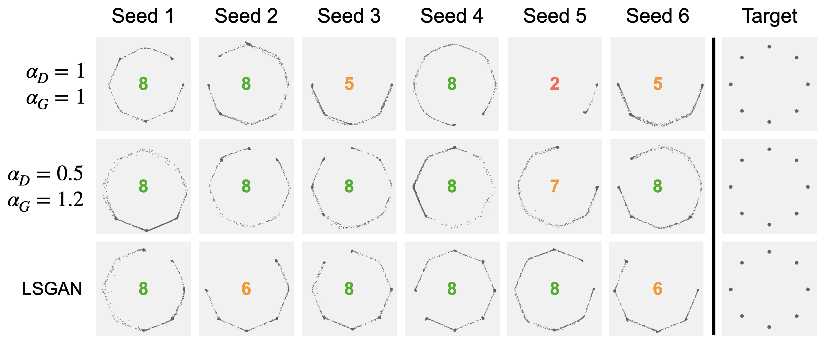
Figure 3: Generated samples from two $(\alpha_{D},\alpha_{G})$-GANs trained with the NS objectives in (5a), (11), as well as the LSGAN. We provide 6 seeds to illustrate the stability in performance for each GAN across multiple runs.

III-B Stacked MNIST

The Stacked MNIST dataset is an enhancement of MNIST [26] as it contains images of size $3\times 28\times 28$, where each RGB channel is a $28\times 28$ image randomly sampled from MNIST. Stacked MNIST is a popular choice for image generation since its use of 3 channels allows for a total of $10^{3}=1000$ modes, as opposed to the 10 modes (digits) in MNIST, which makes the latter much easier for GANs to learn. We generate 100,000 training samples, 25,000 testing samples, and the same number of 100-dimension latent Gaussian noise vectors.

We use the DCGAN architecture [27] for training, which uses deep convolutional neural networks (CNN) for both D and G (details in Tables VII, VII of Appendix E). As in other works, we focus solely on the NS setting using appropriate objective functions for vanilla GAN, $(\alpha_{D},\alpha_{G})$-GAN, and LSGAN. We compute the mode coverage of each trial by feeding each generated sample to a 1000-mode CNN classifier. The classifier is obtained by pretraining on MNIST to achieve 99.5% validation accuracy. We also consider a range of settings for two key hyperparameters: the number of epochs and learning rate for Adam optimization. Each combination of objective function, number of epochs, and learning rate is trained for 100 seeds; this allows us to report the mean mode coverage. We also report the mean Fréchet Inception Distance (FID).

In Fig. 4(a) and 4(b), we empirically demonstrate the dependence of mode coverage on learning rate and number of epochs, respectively (FID plots are in Appendix E-C). Achieving robustness to hyperparameter initialization is highly desirable in the unsupervised GAN setting as the choices that facilitate steady model convergence are not easily determined without prior mode knowledge. Observing the mode coverage of different $(\alpha_{D},\alpha_{G})$-GANs, we find that as the learning rate or training time increases, the performance of both vanilla GAN and LSGAN deteriorates faster than a GAN with $\alpha_{D}=\alpha_{G}>1$ (see Appendix E for additional details that motivate this choice). Finally, as shown in Fig. 5, we observe that the outputs of $(\alpha_{D},\alpha_{G})$-GAN are more consistent and accurate across multiple seeds, relative to LSGAN and vanilla GAN.

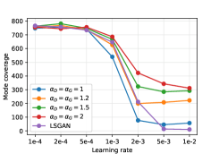
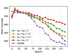
(a)	(b)

Figure 4: Mode coverage vs. (a) varied learning rates with fixed epoch number ($=50$) and (b) varied epoch numbers with fixed learning rate ($=5\times 10^{-4}$) for different GANs, underscoring the vanilla GAN’s hyperparameter sensitivity.

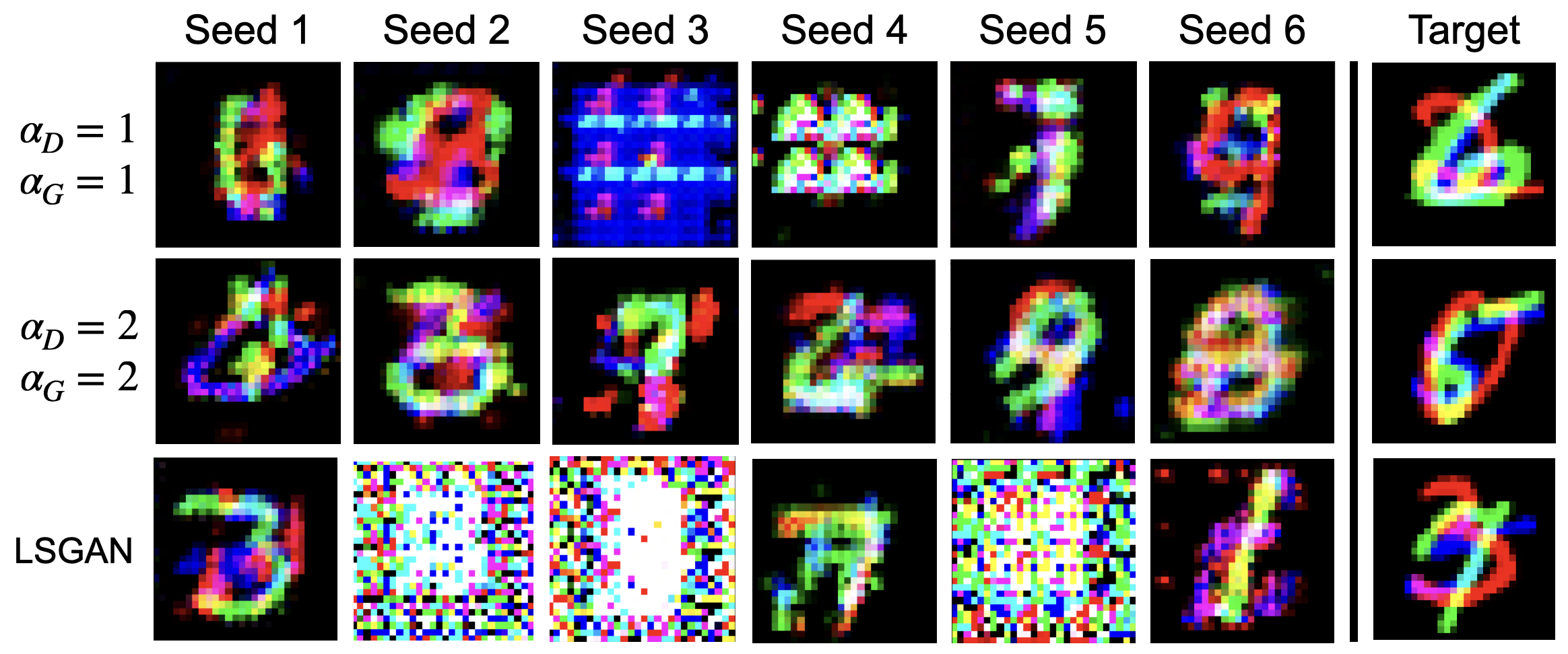
Figure 5: Generated Stacked MNIST samples from three GANs over 6 seeds when trained for 200 epochs with a learning rate of $5\times 10^{-4}$.

IV Concluding Remarks

We have introduced a dual-objective GAN formulation, focusing in particular on using $\alpha$-loss for both players’ objectives. Our results highlight the value of tuning $\alpha$ in alleviating training instabilities and enhancing robustness to learning rates and training epochs, hyperparameters whose optimal values are generally not known a priori. Generalization guarantees of $(\alpha_{D},\alpha_{G})$-GANs is a natural extension to study. An equally important problem is to evaluate if our observations hold more broadly, including, when the training data is noisy [29].

Appendix A Proof of Theorem 1

The proof to obtain (6) is the same as that for [7, Theorem 1], where $\alpha=\alpha_{D}$. The generator’s optimization problem in (5b) with the optimal discriminator in (6) can be written as $\inf_{\theta\in\Theta}V_{\alpha_{G}}(\theta,\omega^{*})$, where

$$V_{\alpha_{G}}(\theta,\omega^{*})$$

$$=\frac{\alpha_{G}}{\alpha_{G}-1}\times$$

$$\left[\int_{\mathcal{X}}\left(p_{r}(x)D_{\omega^{*}}(x)^{\frac{\alpha_{G}-1}{\alpha_{G}}}+p_{G_{\theta}}(x)(1-D_{\omega^{*}}(x))^{\frac{\alpha_{G}-1}{\alpha_{G}}}\right)dx-2\right]$$

$$=\frac{\alpha_{G}}{\alpha_{G}-1}\Bigg{[}\int_{\mathcal{X}}\Bigg{(}p_{r}(x)\left(\frac{p_{r}(x)^{\alpha_{D}}}{p_{r}(x)^{\alpha_{D}}+p_{G_{\theta}}(x)^{\alpha_{D}}}\right)^{\frac{\alpha_{G}-1}{\alpha_{G}}}$$

$$\qquad\qquad\quad+p_{G_{\theta}}(x)\left(\frac{p_{r}(x)^{\alpha_{D}}}{p_{r}(x)^{\alpha_{D}}+p_{G_{\theta}}(x)^{\alpha_{D}}}\right)^{\frac{\alpha_{G}-1}{\alpha_{G}}}\Bigg{)}dx-2\Bigg{]}$$

$$=\frac{\alpha_{G}}{\alpha_{G}-1}\times$$

$$\left(\int_{\mathcal{X}}p_{G_{\theta}}(x)\left(\frac{(p_{r}(x)/p_{G_{\theta}}(x))^{\alpha_{D}(1-1/\alpha_{G})+1}+1}{((p_{r}(x)/p_{G_{\theta}}(x))^{\alpha_{D}}+1)^{1-1/\alpha_{G}}}\right)dx-2\right)$$

$$=\int_{\mathcal{X}}p_{G_{\theta}}(x)f_{\alpha_{D},\alpha_{G}}\left(\frac{p_{r}(x)}{p_{G_{\theta}}(x)}\right)dx+\frac{\alpha_{G}}{\alpha_{G}-1}\left(2^{\frac{1}{\alpha_{G}}}-2\right),$$

where $f_{\alpha_{D},\alpha_{G}}$ is as defined in (7). Note that if $f_{\alpha_{D},\alpha_{G}}$ is strictly convex, the first term in the last equality above equals an $f$-divergence which is minimized if and only if $P_{r}=P_{G_{\theta}}$. Define the regions $R_{1}$ and $R_{2}$ as follows:

$$R_{1}\coloneqq\Big{\{}(\alpha_{D},\alpha_{G})\in(0,\infty]^{2}\bigm{|}\alpha_{D}\leq 1,\alpha_{G}>\frac{\alpha_{D}}{\alpha_{D}+1}\Big{\}}$$

and

$$R_{2}\coloneqq\Big{\{}(\alpha_{D},\alpha_{G})\in(0,\infty]^{2}\bigm{|}\alpha_{D}>1,\frac{\alpha_{D}}{2}<\alpha_{G}\leq\alpha_{D}\Big{\}}.$$

In order to prove that $f_{\alpha_{D},\alpha_{G}}$ is strictly convex for $(\alpha_{D},\alpha_{G})\in R_{1}\cup R_{2}$, we take its second derivative, which yields

$$f^{\prime\prime}_{\alpha_{D},\alpha_{G}}(u)$$

$$=A_{\alpha_{D},\alpha_{G}}(u)\bigg{[}(\alpha_{G}+\alpha_{D}\alpha_{G}-\alpha_{D})\left(u+u^{\alpha_{D}+\frac{\alpha_{D}}{\alpha_{G}}}\right)$$

$$\qquad\qquad\qquad\qquad+(\alpha_{G}-\alpha_{D}\alpha_{G})\left(u^{\frac{\alpha_{D}}{\alpha_{G}}}+u^{\alpha_{D}+1}\right)\bigg{]},$$ (23)

where

$$A_{\alpha_{D},\alpha_{G}}(u)=\frac{\alpha_{D}}{\alpha_{G}}u^{\alpha_{D}-\frac{\alpha_{D}}{\alpha_{G}}-2}(1+u^{\alpha_{D}})^{\frac{1}{\alpha_{G}}-3}.$$ (24)

Note that $A_{\alpha_{D},\alpha_{G}}(u)>0$ for all $u>0$ and $\alpha_{D},\alpha_{G}\in(0,\infty]$. Therefore, in order to ensure $f^{\prime\prime}_{\alpha_{D},\alpha_{G}}(u)>0$ for all $u>0$ it is sufficient to have

$$\alpha_{G}+\alpha_{D}\alpha_{G}-\alpha_{D}>\alpha_{G}(\alpha_{D}-1)B_{\alpha_{D},\alpha_{G}}(u),$$ (25)

where

$$B_{\alpha_{D},\alpha_{G}}(u)=\frac{u^{\frac{\alpha_{D}}{\alpha_{G}}}+u^{\alpha_{D}+1}}{u+u^{\alpha_{D}+\frac{\alpha_{D}}{\alpha_{G}}}}$$ (26)

for $u>0$. Since $B_{\alpha_{D},\alpha_{G}}(u)>0$ for all $u>0$, the sign of the RHS of (25) is determined by whether $\alpha_{D}\leq 1$ or $\alpha_{D}>1$. We look further into these two cases in the following:

Case 1: $\alpha_{D}\leq 1$. Then $\alpha_{G}(\alpha_{D}-1)B_{\alpha_{D},\alpha_{G}}(u)\leq 0$ for all $u>0$ and $(\alpha_{D},\alpha_{G})\in(0,\infty]^{2}$. Therefore, we need

$$\alpha_{G}(1+\alpha_{D})-\alpha_{D}>0\Leftrightarrow\alpha_{G}>\frac{\alpha_{D}}{\alpha_{D}+1}.$$ (27)

Case 2: $\alpha_{D}>1$. Then $\alpha_{G}(\alpha_{D}-1)B_{\alpha_{D},\alpha_{G}}(u)>0$ for all $u>0$ and $(\alpha_{D},\alpha_{G})\in(0,\infty]^{2}$. In order to obtain conditions on $\alpha_{D}$ and $\alpha_{G}$, we determine the monotonicity of $B_{\alpha_{D},\alpha_{G}}$ by finding its first derivative as follows:

$$B^{\prime}_{\alpha_{D},\alpha_{G}}(u)$$

$$=\frac{(\alpha_{G}-\alpha_{D})(u^{2\alpha_{D}}-1)+\alpha_{D}\alpha_{G}\Big{(}u^{\alpha_{D}-\frac{\alpha_{D}}{\alpha_{G}}+1}-u^{\alpha_{D}+\frac{\alpha_{D}}{\alpha_{G}}-1}\Big{)}}{\alpha_{G}u^{-\frac{\alpha_{D}}{\alpha_{G}}}\Big{(}u+u^{\alpha_{D}+\frac{\alpha_{D}}{\alpha_{G}}}\Big{)}^{2}}.$$

Since the denominator of $B^{\prime}_{\alpha_{D},\alpha_{G}}$ is positive for all $u>0$ and $(\alpha_{D},\alpha_{G})\in(0,\infty]^{2}$, we just need to check the sign of the numerator.
Case 2a: $\alpha_{D}>\alpha_{G}$. For $u\in(0,1)$,

$$u^{2\alpha_{D}}-1<0\quad\text{and}\quad u^{\alpha_{D}-\frac{\alpha_{D}}{\alpha_{G}}+1}-u^{\alpha_{D}+\frac{\alpha_{D}}{\alpha_{G}}-1}>0,$$

so $B^{\prime}_{\alpha_{D},\alpha_{G}}(u)>0$. For $u>1$,

$$u^{2\alpha_{D}}-1>0\quad\text{and}\quad u^{\alpha_{D}-\frac{\alpha_{D}}{\alpha_{G}}+1}-u^{\alpha_{D}+\frac{\alpha_{D}}{\alpha_{G}}-1}<0,$$

so $B^{\prime}_{\alpha_{D},\alpha_{G}}(u)<0$. For $u=1$, $B^{\prime}_{\alpha_{D},\alpha_{G}}(u)=0$. Hence, $B^{\prime}_{\alpha_{D},\alpha_{G}}$ is strictly increasing for $u\in(0,1)$ and strictly decreasing for $u\geq 1$. Therefore, $B_{\alpha_{D},\alpha_{G}}$ attains a maximum value of 1 at $u=1$. This means $B_{\alpha_{D},\alpha_{G}}$ is bounded, i.e. $B_{\alpha_{D},\alpha_{G}}\in(0,1]$ for all $u>0$. Thus, in order for (25) to hold, it suffices to ensure that

$$\alpha_{G}+\alpha_{D}\alpha_{G}-\alpha_{D}>\alpha_{G}(\alpha_{D}-1)\Leftrightarrow\alpha_{G}>\frac{\alpha_{G}}{2}.$$ (28)

Case 2b: $\alpha_{D}<\alpha_{G}$. For $u\in(0,1)$, $u^{2\alpha_{D}}-1<0$ and $u^{\alpha_{D}-\frac{\alpha_{D}}{\alpha_{G}}+1}-u^{\alpha_{D}+\frac{\alpha_{D}}{\alpha_{G}}-1}<0$, so $B^{\prime}_{\alpha_{D},\alpha_{G}}(u)<0$. For $u>1$, $u^{2\alpha_{D}}-1>0$ and $u^{\alpha_{D}-\frac{\alpha_{D}}{\alpha_{G}}+1}-u^{\alpha_{D}+\frac{\alpha_{D}}{\alpha_{G}}-1}>0$, so $B^{\prime}_{\alpha_{D},\alpha_{G}}(u)>0$. Hence, $B^{\prime}_{\alpha_{D},\alpha_{G}}$ is strictly decreasing for $u\in(0,1)$ and strictly increasing for $u\geq 1$. Therefore, $B_{\alpha_{D},\alpha_{G}}$ attains a minimum value of 1 at $u=1$. This means that $B_{\alpha_{D},\alpha_{G}}$ is not bounded above, so it is not possible to satisfy (25) without restricting the domain of $B_{\alpha_{D},\alpha_{G}}$.

Thus, for $(\alpha_{D},\alpha_{G})\in R_{1}\cup R_{2}$,

$$V_{\alpha_{G}}(\theta,\omega^{*})=D_{f_{\alpha_{D},\alpha_{G}}}(P_{r}||P_{G_{\theta}})+\frac{\alpha_{G}}{\alpha_{G}-1}\left(2^{\frac{1}{\alpha_{G}}}-2\right).$$

This yields (8). Note that $D_{f_{\alpha_{D},\alpha_{G}}}(P||Q)$ is symmetric since

$$D_{f_{\alpha_{D},\alpha_{G}}}(Q||P)$$

$$=\int_{\mathcal{X}}p(x)f_{\alpha_{D},\alpha_{G}}\left(\frac{q(x)}{p(x)}\right)dx$$

$$=\frac{\alpha_{G}}{\alpha_{G}-1}\times$$

$$\left(\int_{\mathcal{X}}p(x)\left(\frac{(p(x)/q(x))^{-{\alpha_{D}\left(1-\frac{1}{\alpha_{G}}\right)}-1}+1}{((p(x)/q(x))^{-\alpha_{D}}+1)^{1-\frac{1}{\alpha_{G}}}}\right)dx-2^{\frac{1}{\alpha_{G}}}\right)$$

$$=\frac{\alpha_{G}}{\alpha_{G}-1}\times$$

$$\left(\int_{\mathcal{X}}p(x)\left(\frac{q(x)/p(x)+(p(x)/q(x))^{\alpha_{D}\left(1-\frac{1}{\alpha_{G}}\right)}}{(1+(p(x)/q(x))^{\alpha_{D}})^{1-\frac{1}{\alpha_{G}}}}\right)dx-2^{\frac{1}{\alpha_{G}}}\right)$$

$$=\frac{\alpha_{G}}{\alpha_{G}-1}\times$$

$$\left(\int_{\mathcal{X}}q(x)\left(\frac{1+(p(x)/q(x))^{\alpha_{D}\left(1-\frac{1}{\alpha_{G}}\right)}}{(1+(p(x)/q(x))^{\alpha_{D}})^{1-\frac{1}{\alpha_{G}}}}\right)dx-2^{\frac{1}{\alpha_{G}}}\right)$$

$$=D_{f_{\alpha_{D},\alpha_{G}}}(P||Q).$$

Since $f_{\alpha_{D},\alpha_{G}}$ is strictly convex and $f_{\alpha_{D},\alpha_{G}}(1)=0$, $D_{f_{\alpha_{D},\alpha_{G}}}(P_{r}||P_{G_{\theta}})\geq 0$ with equality if and only if $P_{r}=P_{G_{\theta}}$. Thus, we have $V_{\alpha_{G}}(\theta,\omega^{*})\geq\frac{\alpha_{G}}{\alpha_{G}-1}\left(2^{\frac{1}{\alpha_{G}}}-2\right)$ with equality if and only if $P_{r}=P_{G_{\theta}}$.

Appendix B Proof of Theorem 2

The generator’s optimization problem in (5b) with the optimal discriminator in (6) can be written as $\inf_{\theta\in\Theta}V^{\text{NS}}_{\alpha_{G}}(\theta,\omega^{*})$, where

$$V^{\text{NS}}_{\alpha_{G}}(\theta,\omega^{*})$$

$$=\frac{\alpha_{G}}{\alpha_{G}-1}\left[1-\int_{\mathcal{X}}\left(p_{G_{\theta}}(x)D_{\omega^{*}}(x)^{\frac{\alpha_{G}-1}{\alpha_{G}}}\right)dx\right]$$

$$=\frac{\alpha_{G}}{\alpha_{G}-1}\Bigg{[}1-\int_{\mathcal{X}}p_{G_{\theta}}(x)\left(\frac{p_{r}(x)^{\alpha_{D}}}{p_{r}(x)^{\alpha_{D}}+p_{G_{\theta}}(x)^{\alpha_{D}}}\right)^{\frac{\alpha_{G}-1}{\alpha_{G}}}dx\Bigg{]}$$

$$=\frac{\alpha_{G}}{\alpha_{G}-1}\Bigg{[}1-\int_{\mathcal{X}}p_{G_{\theta}}(x)\frac{(p_{r}(x)/p_{G_{\theta}}(x))^{\alpha_{D}(1-1/\alpha_{G})}}{((p_{r}(x)/p_{G_{\theta}}(x))^{\alpha_{D}}+1)^{1-1/\alpha_{G}}}dx\Bigg{]}$$

$$=\int_{\mathcal{X}}p_{G_{\theta}}(x)f^{\text{NS}}_{\alpha_{D},\alpha_{G}}\left(\frac{p_{r}(x)}{p_{G_{\theta}}(x)}\right)dx+\frac{\alpha_{G}}{\alpha_{G}-1}\left(1-2^{\frac{1}{\alpha_{G}}-1}\right),$$

where $f^{\text{NS}}_{\alpha_{D},\alpha_{G}}$ is as defined in (12). In order to prove that $f^{\text{NS}}_{\alpha_{D},\alpha_{G}}$ is strictly convex for $(\alpha_{D},\alpha_{G})\in R_{\text{NS}}=\{(\alpha_{D},\alpha_{G})\in(0,\infty]^{2}\mid\alpha_{D}>\alpha_{G}(\alpha_{D}-1)\}$, we take its second derivative, which yields

$$f^{\prime\prime}_{\alpha_{D},\alpha_{G}}(u)$$

$$=A_{\alpha_{D},\alpha_{G}}(u)\bigg{[}(\alpha_{G}-\alpha_{D}\alpha_{G}+\alpha_{D})+\alpha_{G}(1+\alpha_{D})u^{\alpha_{D}}\bigg{]},$$ (29)

where $A_{\alpha_{D},\alpha_{G}}$ is defined as in (24). Since $A_{\alpha_{D},\alpha_{G}}(u)>0$ for all $u>0$ and $(\alpha_{D},\alpha_{G})\in(0,\infty]^{2}$, to ensure $f^{\prime\prime}_{\alpha_{D},\alpha_{G}}(u)>0$ for all $u>0$ it suffices to have

$$\frac{\alpha_{G}-\alpha_{D}\alpha_{G}+\alpha_{D}}{\alpha_{G}(1+\alpha_{D})}>-u^{\alpha_{D}}$$

for all $u>0$. This is equivalent to

$$\frac{\alpha_{G}-\alpha_{D}\alpha_{G}+\alpha_{D}}{\alpha_{G}(1+\alpha_{D})}>0,$$

which results in the condition

$$\alpha_{D}>\alpha_{G}(\alpha_{D}-1)$$

for $(\alpha_{D},\alpha_{G})\in(0,\infty]^{2}$. Thus, for $(\alpha_{D},\alpha_{G})\in R_{\text{NS}}$,

$$V^{\text{NS}}_{\alpha_{G}}(\theta,\omega^{*})=D_{f^{\text{NS}}_{\alpha_{D},\alpha_{G}}}(P_{r}||P_{G_{\theta}})+\frac{\alpha_{G}}{\alpha_{G}-1}\left(1-2^{\frac{1}{\alpha_{G}}-1}\right).$$

This yields (13). Note that $D_{f^{\text{NS}}_{\alpha_{D},\alpha_{G}}}(P||Q)$ is not symmetric since $D_{f^{\text{NS}}_{\alpha_{D},\alpha_{G}}}(P||Q)\neq D_{f^{\text{NS}}_{\alpha_{D},\alpha_{G}}}(Q||P)$. Since $f^{\text{NS}}_{\alpha_{D},\alpha_{G}}$ is strictly convex and $f^{\text{NS}}_{\alpha_{D},\alpha_{G}}(1)=0$, $D_{f^{\text{NS}}_{\alpha_{D},\alpha_{G}}}(P_{r}||P_{G_{\theta}})\geq 0$ with equality if and only if $P_{r}=P_{G_{\theta}}$. Thus, we have $V^{\text{NS}}_{\alpha_{G}}(\theta,\omega^{*})\geq\frac{\alpha_{G}}{\alpha_{G}-1}\left(1-2^{\frac{1}{\alpha_{G}}-1}\right)$ with equality if and only if $P_{r}=P_{G_{\theta}}$.

Appendix C Proof of Theorem 3

By adding and subtracting relevant terms, we obtain

$$d_{\omega^{*}(P_{r},P_{G_{\hat{\theta}^{*}}})}(P_{r},{P}_{G_{\hat{\theta}^{*}}})-\inf_{\theta\in\Theta}d_{\omega^{*}(P_{r},P_{G_{\theta}})}(P_{r},P_{G_{\theta}})$$

$$=d_{\omega^{*}(P_{r},P_{G_{\hat{\theta}^{*}}})}(P_{r},{P}_{G_{\hat{\theta}^{*}}})-d_{\omega^{*}(P_{r},P_{G_{\hat{\theta}^{*}}})}(\hat{P}_{r},{P}_{G_{\hat{\theta}^{*}}})$$ (30a)

$$\quad+\inf_{\theta\in\Theta}d_{\omega^{*}(P_{r},P_{G_{\theta}})}(\hat{P}_{r},P_{G_{\theta}})-\inf_{\theta\in\Theta}d_{\omega^{*}(P_{r},P_{G_{\theta}})}(P_{r},P_{G_{\theta}})$$ (30b)

$$\quad+d_{\omega^{*}(P_{r},P_{G_{\hat{\theta}^{*}}})}(\hat{P}_{r},{P}_{G_{\hat{\theta}^{*}}})-\inf_{\theta\in\Theta}d_{\omega^{*}(P_{r},P_{G_{\theta}})}(\hat{P}_{r},P_{G_{\theta}}).$$ (30c)

We upper-bound (30) in the following three steps. Let $\phi(\cdot)=-\ell_{\alpha_{G}}(1,\cdot)$ and $\psi(\cdot)=-\ell_{\alpha_{G}}(0,\cdot)$.

We first upper-bound (30a). Let $\omega^{*}(\hat{\theta}^{*})=\omega^{*}(P_{r},P_{G_{\hat{\theta}^{*}}})$. Using (15) yields

$$d_{\omega^{*}(P_{r},P_{G_{\hat{\theta}^{*}}})}(P_{r},{P}_{G_{\hat{\theta}^{*}}})-d_{\omega^{*}(P_{r},P_{G_{\hat{\theta}^{*}}})}(\hat{P}_{r},{P}_{G_{\hat{\theta}^{*}}})$$

$$=\mathbb{E}_{X\sim P_{r}}[\phi(D_{\omega^{*}(\hat{\theta}^{*})}(X))]+\mathbb{E}_{X\sim P_{G_{\hat{\theta}^{*}}}}[\psi(D_{\omega^{*}(\hat{\theta}^{*})}(X))]$$

$$\quad-\left(\mathbb{E}_{X\sim\hat{P}_{r}}[\phi(D_{\omega^{*}(\hat{\theta}^{*})}(X))]+\mathbb{E}_{X\sim P_{G_{\hat{\theta}^{*}}}}[\psi(D_{\omega^{*}(\hat{\theta}^{*})}(X))]\right)$$

$$\leq\left|\mathbb{E}_{X\sim P_{r}}[\phi(D_{\omega^{*}(\hat{\theta}^{*})}(X))]-\mathbb{E}_{X\sim\hat{P}_{r}}[\phi(D_{\omega^{*}(\hat{\theta}^{*})}(X))]\right|$$

$$\leq\sup_{\omega\in\Omega}\left|\mathbb{E}_{X\sim P_{r}}[\phi(D_{\omega}(X))]-\mathbb{E}_{X\sim\hat{P}_{r}}[\phi(D_{\omega}(X))]\right|.$$ (31)

Next, we upper-bound (30b). Let $\theta^{*}=\arg\min_{\theta\in\Theta}d_{\omega^{*}(P_{r},P_{G_{{\theta}}})}(P_{r},{P}_{G_{{\theta}}})$ and $\omega^{*}({\theta}^{*})=\omega^{*}(P_{r},P_{G_{{\theta}^{*}}})$. Then

$$\inf_{\theta\in\Theta}d_{\omega^{*}(P_{r},P_{G_{{\theta}}})}(\hat{P}_{r},P_{G_{\theta}})-\inf_{\theta\in\Theta}d_{\omega^{*}(P_{r},P_{G_{{\theta}}})}(P_{r},P_{G_{\theta}})$$

$$\leq d_{\omega^{*}(\theta^{*})}(\hat{P}_{r},P_{G_{\theta^{*}}})-d_{\omega^{*}(\theta^{*})}(P_{r},P_{G_{\theta^{*}}})$$

$$=\mathbb{E}_{X\sim\hat{P}_{r}}[\phi(D_{\omega^{*}({\theta}^{*})}(X))]+\mathbb{E}_{X\sim P_{G_{{\theta}^{*}}}}[\psi(D_{\omega^{*}({\theta}^{*})}(X))]$$

$$\quad-\left(\mathbb{E}_{X\sim{P}_{r}}[\phi(D_{\omega^{*}({\theta}^{*})}(X))]+\mathbb{E}_{X\sim P_{G_{{\theta}^{*}}}}[\psi(D_{\omega^{*}({\theta}^{*})}(X))]\right)$$

$$=\mathbb{E}_{X\sim\hat{P}_{r}}[\phi(D_{\omega^{*}({\theta}^{*})}(X))]-\mathbb{E}_{X\sim{P}_{r}}[\phi(D_{\omega^{*}({\theta}^{*})}(X))]$$

$$\leq\sup_{\omega\in\Omega}\left|\mathbb{E}_{X\sim P_{r}}[\phi(D_{\omega}(X))]-\mathbb{E}_{X\sim\hat{P}_{r}}[\phi(D_{\omega}(X))]\right|.$$ (32)

Lastly, we upper-bound (30c). Let $\tilde{\theta}=\arg\min_{\theta\in\Theta}d_{\omega^{*}(P_{r},P_{G_{\theta}})}(\hat{P}_{r},{P}_{G_{{\theta}}})$ and $\omega^{*}(\tilde{\theta})=\omega^{*}(P_{r},P_{G_{\tilde{\theta}}})$. Then

$$d_{\omega^{*}(P_{r},P_{G_{\hat{\theta}^{*}}})}(\hat{P}_{r},{P}_{G_{\hat{\theta}^{*}}})-\inf_{\theta\in\Theta}d_{\omega^{*}(P_{r},P_{G_{\theta}})}(\hat{P}_{r},P_{G_{\theta}})$$

$$=d_{\omega^{*}(\hat{\theta}^{*})}(\hat{P}_{r},{P}_{G_{\hat{\theta}^{*}}})-d_{\omega^{*}({\tilde{\theta}})}(\hat{P}_{r},\hat{P}_{G_{\tilde{\theta}}})$$

$$\quad+d_{\omega^{*}({\tilde{\theta}})}(\hat{P}_{r},\hat{P}_{G_{\tilde{\theta}}})-d_{\omega^{*}(\tilde{\theta})}(\hat{P}_{r},P_{G_{\tilde{\theta}}})$$

$$\leq d_{\omega^{*}(\hat{\theta}^{*})}(\hat{P}_{r},{P}_{G_{\hat{\theta}^{*}}})-d_{\omega^{*}({\hat{\theta}^{*}})}(\hat{P}_{r},\hat{P}_{G_{\hat{\theta}^{*}}})$$

$$\quad+d_{\omega^{*}({\tilde{\theta}})}(\hat{P}_{r},\hat{P}_{G_{\tilde{\theta}}})-d_{\omega^{*}(\tilde{\theta})}(\hat{P}_{r},P_{G_{\tilde{\theta}}})$$

$$=\mathbb{E}_{X\sim\hat{P}_{r}}[\phi(D_{\omega^{*}(\hat{\theta}^{*})}(X))]+\mathbb{E}_{X\sim P_{G_{\hat{\theta}^{*}}}}[\psi(D_{\omega^{*}(\hat{\theta}^{*})}(X))]$$

$$\quad-\left(\mathbb{E}_{X\sim\hat{P}_{r}}[\phi(D_{\omega^{*}(\hat{\theta}^{*})}(X))]+\mathbb{E}_{X\sim\hat{P}_{G_{\hat{\theta}^{*}}}}[\psi(D_{\omega^{*}(\hat{\theta}^{*})}(X))]\right)$$

$$\quad+\mathbb{E}_{X\sim\hat{P}_{r}}[\phi(D_{\omega^{*}(\tilde{\theta})}(X))]+\mathbb{E}_{X\sim\hat{P}_{G_{\tilde{\theta}}}}[\psi(D_{\omega^{*}(\tilde{\theta})}(X))]$$

$$\quad-\left(\mathbb{E}_{X\sim\hat{P}_{r}}[\phi(D_{\omega^{*}(\tilde{\theta})}(X))]+\mathbb{E}_{X\sim{P}_{G_{\tilde{\theta}}}}[\psi(D_{\omega^{*}(\tilde{\theta})}(X))]\right)$$

$$=\mathbb{E}_{X\sim P_{G_{\hat{\theta}^{*}}}}[\psi(D_{\omega^{*}(\hat{\theta}^{*})}(X))]-\mathbb{E}_{X\sim\hat{P}_{G_{\hat{\theta}^{*}}}}[\psi(D_{\omega^{*}(\hat{\theta}^{*})}(X))]$$

$$\quad+\mathbb{E}_{X\sim\hat{P}_{G_{\tilde{\theta}}}}[\psi(D_{\omega^{*}(\tilde{\theta})}(X))]-\mathbb{E}_{X\sim{P}_{G_{\tilde{\theta}}}}[\psi(D_{\omega^{*}(\tilde{\theta})}(X))]$$

$$\leq 2\sup_{\omega\in\Omega,\theta\in\Theta}\left|\mathbb{E}_{X\sim P_{G_{{\theta}}}}[\psi(D_{\omega}(X))]-\mathbb{E}_{X\sim\hat{P}_{G_{{\theta}}}}[\psi(D_{\omega}(X))]\right|.$$ (33)

Combining (31)-(33), we obtain the following bound for (30):

$$d_{\omega^{*}(P_{r},P_{G_{\hat{\theta}^{*}}})}(P_{r},{P}_{G_{\hat{\theta}^{*}}})-\inf_{\theta\in\Theta}d_{\omega^{*}(P_{r},P_{G_{\theta}})}(P_{r},P_{G_{\theta}})$$

$$\leq 2\sup_{\omega\in\Omega}\Big{|}\mathbb{E}_{X\sim P_{r}}[\phi(D_{\omega}(X))]-\mathbb{E}_{X\sim\hat{P}_{r}}[\phi(D_{\omega}(X))]\Big{|}$$

$$\quad+2\sup_{\omega\in\Omega,\theta\in\Theta}\Big{|}\mathbb{E}_{X\sim P_{G_{{\theta}}}}[\psi(D_{\omega}(X))]-\mathbb{E}_{X\sim\hat{P}_{G_{{\theta}}}}[\psi(D_{\omega}(X))]\Big{|}$$

$$=2\sup_{\omega\in\Omega}\Big{|}\mathbb{E}_{X\sim P_{r}}[\phi(D_{\omega}(X))]-\frac{1}{n}\sum_{i=1}^{n}\phi(D_{\omega}(X_{i}))\Big{|}$$

$$\quad+2\sup_{\omega\in\Omega,\theta\in\Theta}\Big{|}\mathbb{E}_{X\sim P_{G_{{\theta}}}}[\psi(D_{\omega}(X))]-\frac{1}{m}\sum_{j=1}^{m}\psi(D_{\omega}(X_{j}))\Big{|}.$$ (34)

Note that (34) is exactly the same bound as that in [30, Equation (35)]. Hence, the remainder of the proof follows from the proof of [30, Theorem 3], where $\alpha=\alpha_{G}$.

Appendix D Proof of Theorem 4

Let $\phi(\cdot)=-\ell_{\alpha}(1,\cdot)$ and consider the following modified version of $d^{\ell_{\alpha}}_{\mathcal{F}_{nn}}(\cdot,\cdot)$ (defined in [8, eq. (13)]):

$$d^{\ell_{\alpha}}_{\mathcal{F}_{nn}}(P,Q)=$$

$$\sup_{\omega\in\Omega}\Big{(}\mathbb{E}_{X\sim P}[\phi(D_{\omega}(X))]+\mathbb{E}_{X\sim Q}[\phi(1-D_{\omega}(X))]\Big{)}-2\phi(1/2),$$

where

$$D_{\omega}(x)=\sigma\left(\mathbf{w}_{k}^{\mathsf{T}}r_{k-1}(\mathbf{W}_{d-1}r_{k-2}(\dots r_{1}(\mathbf{W}_{1}(x)))\right)\coloneqq\sigma\left(f_{\omega}(x)\right).$$

Taking $\alpha\to\infty$, we obtain

$$d^{\ell_{\infty}}_{\mathcal{F}_{nn}}(P,Q)=\sup_{\omega\in\Omega}\Big{(}\mathbb{E}_{X\sim P}[D_{\omega}(X)]-\mathbb{E}_{X\sim Q}[D_{\omega}(X)]\Big{)}.$$ (35)

We first prove that $d^{\ell_{\infty}}_{\mathcal{F}_{nn}}$ is a semi-metric.
Claim 1: For any distribution pair $(P,Q)$, $d^{\ell_{\infty}}_{\mathcal{F}_{nn}}(P,Q)\geq 0$.

Proof.

Consider a discriminator which always outputs 1/2, i.e., $D_{\omega}(x)=1/2$ for all $x$. Note that such a neural network discriminator exists, as setting $\mathbf{w}_{k}=0$ results in $D_{\omega}(x)=\sigma(0)=0$. For this discriminator, the objective function in (35) evaluates to $1/2-1/2=0$. Since $d^{\ell_{\infty}}_{\mathcal{F}_{nn}}$ is a supremum over all discriminators, we have $d^{\ell_{\infty}}_{\mathcal{F}_{nn}}(P,Q)\geq 0$.

Claim 2: For any distribution pair $(P,Q)$, $d^{\ell_{\infty}}_{\mathcal{F}_{nn}}(P,Q)=d^{\ell_{\infty}}_{\mathcal{F}_{nn}}(Q,P)$.

Proof.

$$d^{\ell_{\infty}}_{\mathcal{F}_{nn}}(P,Q)$$

$$=\sup_{\omega\in\Omega}\Big{(}\mathbb{E}_{X\sim P}[D_{\omega}(X)]-\mathbb{E}_{X\sim Q}[D_{\omega}(X)]\Big{)}$$

$$=\sup_{\mathbf{W}_{1},\dots,\mathbf{w}_{k}}\Big{(}\mathbb{E}_{X\sim P}[D_{\omega}(X)]-\mathbb{E}_{X\sim Q}[D_{\omega}(X)]\Big{)}$$

$$\overset{(i)}{=}\sup_{\mathbf{W}_{1},\dots,-\mathbf{w}_{k}}\Big{(}\mathbb{E}_{X\sim P}[\sigma\left(-f_{\omega}(x)\right)]-\mathbb{E}_{X\sim Q}[\sigma\left(-f_{\omega}(x)\right)]\Big{)}$$

$$\overset{(ii)}{=}\sup_{\mathbf{W}_{1},\dots,\mathbf{w}_{k}}\Big{(}\mathbb{E}_{X\sim P}[1-\sigma\left(f_{\omega}(x)\right)]-\mathbb{E}_{X\sim Q}[1-\sigma\left(f_{\omega}(x)\right)]\Big{)}$$

$$=\sup_{\mathbf{W}_{1},\dots,\mathbf{w}_{k}}\Big{(}\mathbb{E}_{X\sim Q}[\sigma\left(f_{\omega}(x)\right)]-\mathbb{E}_{X\sim P}[\sigma\left(f_{\omega}(x)\right)]\Big{)}$$

$$=d^{\ell_{\infty}}_{\mathcal{F}_{nn}}(Q,P),$$

where $(i)$ follows from replacing $\mathbf{w}_{k}$ with $-\mathbf{w}_{k}$ and $(ii)$ follows from the sigmoid property $\sigma(-x)=1-\sigma(x)$ for all $x$.

Claim 3: For any distribution $P$, $d^{\ell_{\infty}}_{\mathcal{F}_{nn}}(P,P)=0$.

Proof.

$$d^{\ell_{\infty}}_{\mathcal{F}_{nn}}(P,P)=\sup_{\omega\in\Omega}\Big{(}\mathbb{E}_{X\sim P}[D_{\omega}(X)]-\mathbb{E}_{X\sim P}[D_{\omega}(X)]\Big{)}=0.$$

Claim 4: For any distributions $P,Q,R$, $d^{\ell_{\infty}}_{\mathcal{F}_{nn}}(P,Q)\leq d^{\ell_{\infty}}_{\mathcal{F}_{nn}}(P,R)+d^{\ell_{\infty}}_{\mathcal{F}_{nn}}(R,Q)$.

Proof.

$$d^{\ell_{\infty}}_{\mathcal{F}_{nn}}(P,Q)$$

$$=\sup_{\omega\in\Omega}\Big{(}\mathbb{E}_{X\sim P}[D_{\omega}(X)]-\mathbb{E}_{X\sim Q}[D_{\omega}(X)]\Big{)}$$

$$=\sup_{\omega\in\Omega}\Big{(}\mathbb{E}_{X\sim P}[D_{\omega}(X)]-\mathbb{E}_{X\sim R}[D_{\omega}(X)]$$

$$\qquad\qquad\quad+\mathbb{E}_{X\sim R}[D_{\omega}(X)]-\mathbb{E}_{X\sim Q}[D_{\omega}(X)]\Big{)}$$

$$\leq\sup_{\omega\in\Omega}\Big{(}\mathbb{E}_{X\sim P}[D_{\omega}(X)]-\mathbb{E}_{X\sim R}[D_{\omega}(X)]\Big{)}$$

$$\qquad+\sup_{\omega\in\Omega}\Big{(}\mathbb{E}_{X\sim R}[D_{\omega}(X)]-\mathbb{E}_{X\sim Q}[D_{\omega}(X)]\Big{)}$$

$$=d^{\ell_{\infty}}_{\mathcal{F}_{nn}}(P,R)+d^{\ell_{\infty}}_{\mathcal{F}_{nn}}(R,Q).$$

Thus, $d^{\ell_{\infty}}_{\mathcal{F}_{nn}}$ is a semi-metric. The remaining part of the proof of the lower bound follows along the same lines as that of [18, Theorem 2] by an application of Fano’s inequality [31, Theorem 2.5] (that requires the involved divergence measure to be a semi-metric), replacing $d_{\mathcal{F}_{nn}}$ with $d^{\ell_{\infty}}_{\mathcal{F}_{nn}}$ and noting that the additional sigmoid activation function after the last layer in the discriminator satisfies the monotonicity assumption so that $C(\mathcal{P}(\mathcal{X}))>0$ (for $C(\mathcal{P}(\mathcal{X}))$ defined in (22)).

Appendix E Additional Experimental Results

E-A Brief Overview of LSGAN

The Least Squares GAN (LSGAN) is a dual-objective min-max game introduced in [15]. The LSGAN objective functions, as the name suggests, involve squared loss functions for D and G which are written as

$$\sup_{\omega\in\Omega}\;\frac{1}{2}\Big{(}\mathbb{E}_{X\sim P_{r}}[(D_{\omega}(X)-b)^{2}]+\mathbb{E}_{X\sim P_{G_{\theta}}}[(D_{\omega}(X)-a)^{2}]\Big{)}$$

$$\inf_{\theta\in\Theta}\;\frac{1}{2}\Big{(}\mathbb{E}_{X\sim P_{r}}[(D_{\omega}(X)-c)^{2}]+\mathbb{E}_{X\sim P_{G_{\theta}}}[(D_{\omega}(X)-c)^{2}]\Big{)}.$$ (36)

The parameters $a$, $b$, and $c$ are chosen such that (36) reduces to minimizing the Pearson $\chi^{2}$-divergence between $P_{r}+P_{G_{\theta}}$ and $2P_{G_{\theta}}$. As done in the original paper [15], we use $a=1$, $b=0$ and $c=1$ for our experiments to make fair comparisons. The authors refer to this choice of parameters as the 0-1 binary coding scheme.

E-B 2D Gaussian Mixture Ring

In Tables III and III, we report the success (8/8 mode coverage) and failure (0/8 mode coverage) rates over 200 seeds for a grid of $(\alpha_{D},\alpha_{G})$ combinations for the saturating setting. Compared to the vanilla GAN performance, we find that tuning $\alpha_{D}$ below 1 leads to a greater success rate and lower failure rate. However, in this saturating loss setting, we find that tuning $\alpha_{G}$ away from 1 has no significant impact on GAN performance.

TABLE I: Success rates for 2D-ring with the Saturating $(\alpha_{D},\alpha_{G})$-GAN over 200 seeds, with top 4 combinations emboldened.

% of success (8/8 modes)		$\alpha_{D}$
		0.5	0.6	0.7	0.8	0.9	1.0
$\alpha_{G}$	0.9	73	79	69	60	46	34
	1.0	80	79	74	68	54	47
	1.1	79	77	68	70	59	47
	1.2	75	74	71	65	57	46

TABLE II: Failure rates for 2D-ring with the Saturating $(\alpha_{D},\alpha_{G})$-GAN over 200 seeds, with top 3 combinations emboldened.

% of failure (0/8 modes)		$\alpha_{D}$
		0.5	6	7	0.8	0.9	1.0
$\alpha_{G}$	0.9	11	10	12	13	29	49
	1.0	5	5	7	8	16	30
	1.1	7	9	13	12	13	26
	1.2	9	5	9	12	17	31

TABLE III: Success rates for 2D-ring with the NS $(\alpha_{D},\alpha_{G})$-GAN over 200 seeds, with top 5 combinations emboldened.

% of success (8/8 modes)		$\alpha_{D}$
		0.5	0.6	0.7	0.8	0.9	1.0	1.1	1.2
$\alpha_{G}$	0.8	35	24	19	19	14	16	18	10
	0.9	39	37	19	22	16	20	19	21
	1.0	34	35	29	28	26	22	20	32
	1.1	40	36	31	22	24	15	23	25
	1.2	45	38	34	25	26	28	20	22
	1.3	44	39	26	28	28	25	31	29

In Table III, we detail the success rates for the NS setting. We note that for this dataset, no failures, and therefore, no vanishing/exploding gradients, occurred in the NS setting. In particular, we find that the $(0.5,1.2)$-GAN doubles the success rate of the vanilla $(1,1)$-GAN, which is more susceptible to mode collapse as illustrated in Figure 3. We also find that LSGAN achieves a success rate of 32.5%, which is greater than vanilla GAN but less than the best-performing $(\alpha_{D},\alpha_{G})$-GAN.

E-C Stacked MNIST

For the Stacked MNIST dataset, the discriminator and generator architectures we use are outlined in Tables VII and VII, respectively. Both involve four CNN layers whose parameters, include kernel size (i.e., the size of the filter which we denote by Kernel), stride (the number of pixels that the filter moves by), and the output activation functions for each layer. We assume zero padding. Finally, BN in Tables VII and VII refers to batch normalization, a technique of normalizing the inputs to each layer where the normalization is over a batch of samples used to train the model at any time. This approach is common in deep learning to avoid cumulative floating point errors and overflows and keep all features in the same range, thereby serving as a computational tool to avoid vanishing and/or exploding gradients.

TABLE IV: Discriminator architecture for Stacked MNIST.
The final sigmoid activation layer is removed for LSGAN.

Layer	Output size	Kernel	Stride	BN	Activation
Input	$3\times 28\times 28$
Convolution	$8\times 14\times 14$	$3\times 3$	2	Yes	LeakyReLU
Convolution	$16\times 7\times 7$	$3\times 3$	2	Yes	LeakyReLU
Convolution	$32\times 3\times 3$	$3\times 3$	2	Yes	LeakyReLU
Convolution	$1\times 1\times 1$	$3\times 3$	2		Sigmoid

TABLE V: Generator architecture for the Stacked MNIST experiment.

Layer	Output size	Kernel	Stride	BN	Activation
Input	$100\times 1\times 1$
ConvTranspose	$32\times 3\times 3$	$3\times 3$	2	Yes	ReLU
ConvTranspose	$16\times 7\times 7$	$3\times 3$	2	Yes	ReLU
ConvTranspose	$8\times 14\times 14$	$3\times 3$	2	Yes	ReLU
ConvTranspose	$3\times 28\times 28$	$3\times 3$	2		Tanh

TABLE VI: Mean mode coverage reported over 100 seeds for $(\alpha_{D},\alpha_{G})$-GAN trained on Stacked MNIST with a learning rate of $10^{-3}$ for 50 epochs. The best results are shown in bold.

Mode coverage		$\alpha_{D}$
		0.9	1	1.1	1.2
$\alpha_{G}$	1	502	541	480	508
	1.2	619	586	580	598
	1.5	648	684	689	645
	2	676	690	703	685

TABLE VII: Mean mode coverage reported over 100 seeds for $(\alpha_{D},\alpha_{G})$-GAN trained on Stacked MNIST with a learning rate of $5\times 10^{-4}$ for 100 epochs. The best results are shown in bold.

Mode coverage		$\alpha_{D}$
		1	2
$\alpha_{G}$	1	665	645
	2	693	724

In the main document, we demonstrated the dependence of the computed mode coverage on both the learning rate and the number of training epochs. We now illustrate a commonly used metric for evaluating the quality of the synthetic data, namely, the Frechét Inception Distance (FID). In theory, the FID quantifies the 2-Wasserstein distance between the two distributions, and thus, it is desirable to achieve small values for the FID. In practice, FID is computed using a lower dimensional latent space for both the real and synthetic images, preferably at a layer close to the output layer. The InceptionNet-V3 deep learning model [28] is used to extract such low-dimensional latent features and use the mean and variance of the features at that layer to compute the FID.

In Fig. 6(a) and 6(b), we plot the FID as a function of the learning rate and the number of epochs, respectively. For each such plot, we compare the FID scores for the vanilla GAN ($\alpha_{D}=\alpha_{G}=1)$ and LSGAN against different ($\alpha_{D}=\alpha_{G}>1)$ values. For these plots, note that we set $\alpha_{D}=\alpha_{G}$. Our motivation for doing so is based on the results shown in Table VII and VII, where Table VII captures the mode coverage for a learning rate of $10^{-3}$ and over 50 training epochs and Table VII captures the mode coverage for a learning rate of $5\times 10^{-4}$ and over 100 training epochs. Our results consistently suggest that $\alpha_{G}$ has a larger impact on the GAN mode coverage performance than $\alpha_{D}$. For both of the abovementioned hyperparameter choices, our results show that $\alpha_{G}=2$ achieves a wide mode coverage no matter the choice of $\alpha_{D}>1$; thus, we simplify the $(\alpha_{D},\alpha_{G})$ search by setting $\alpha_{D}=\alpha_{G}$. Higher values for $\alpha_{D}$ and $\alpha_{G}$ work to mitigate gradient explosion as the derivative of $\alpha$-loss ($\ell_{a}(x)$) approaches 1 as $x\rightarrow 0$ and $\alpha\rightarrow\infty$.

We observe that for smaller values of the learning rate, the FID scores are similar across the GANs; interestingly, we observe a similar trend for lower number of epochs. However, when we increase the learning rate or the number of epochs, the FIDs for vanilla (i.e., $(1,1)$-GAN) and LSGAN increase at a much greater rate than those of the $(\alpha_{D},\alpha_{G}>1)$-GANs. These results show that tuning $\alpha_{D}$ and $\alpha_{G}$ above 1 can desensitize the GAN training to hyperparameter initialization, which is particularly desirable when evaluating GANs without prior mode knowledge, as is often the case in practice.

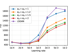
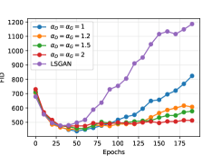
(a)	(b)

Figure 6: FID vs. (a) varied learning rates with fixed epoch numbers ($=50$) and (b) varied epoch numbers with fixed learning rate ($=5\times 10^{-4}$) for different GANs, underscoring the vanilla GAN’s hyperparameter sensitivity.

References

- [1] I. J. Goodfellow, J. Pouget-Abadie, M. Mirza, B. Xu, D. Warde-Farley, S. Ozair, A. Courville, and Y. Bengio, “Generative adversarial nets,” in Proceedings of the 27th International Conference on Neural Information Processing Systems - Volume 2, 2014, p. 2672–2680.
- [2] J. Lin, “Divergence measures based on the Shannon entropy,” IEEE Transactions on Information Theory, vol. 37, no. 1, pp. 145–151, 1991.
- [3] S. Nowozin, B. Cseke, and R. Tomioka, “-GAN: Training generative neural samplers using variational divergence minimization,” in Proceedings of the 30th International Conference on Neural Information Processing Systems, 2016, p. 271–279.
- [4] M. Arjovsky, S. Chintala, and L. Bottou, “Wasserstein generative adversarial networks,” in Proceedings of the 34th International Conference on Machine Learning, vol. 70, 2017, pp. 214–223.
- [5] B. K. Sriperumbudur, K. Fukumizu, A. Gretton, B. Schölkopf, and G. R. Lanckriet, “On the empirical estimation of integral probability metrics,” Electronic Journal of Statistics, vol. 6, pp. 1550–1599, 2012.
- [6] T. Liang, “How well generative adversarial networks learn distributions,” arXiv preprint arXiv:1811.03179, 2018.
- [7] G. R. Kurri, T. Sypherd, and L. Sankar, “Realizing GANs via a tunable loss function,” in IEEE Information Theory Workshop (ITW), 2021, pp. 1–6.
- [8] G. R. Kurri, M. Welfert, T. Sypherd, and L. Sankar, “-GAN: Convergence and estimation guarantees,” in IEEE International Symposium on Information Theory (ISIT), 2022, pp. 276–281.
- [9] T. Sypherd, M. Diaz, L. Sankar, and P. Kairouz, “A tunable loss function for binary classification,” in IEEE International Symposium on Information Theory, 2019, pp. 2479–2483.
- [10] T. Sypherd, M. Diaz, J. K. Cava, G. Dasarathy, P. Kairouz, and L. Sankar, “A tunable loss function for robust classification: Calibration, landscape, and generalization,” IEEE Transactions on Information Theory, vol. 68, no. 9, pp. 6021–6051, 2022.
- [11] F. Österreicher, “On a class of perimeter-type distances of probability distributions,” Kybernetika, vol. 32, no. 4, pp. 389–393, 1996.
- [12] F. Liese and I. Vajda, “On divergences and informations in statistics and information theory,” IEEE Transactions on Information Theory, vol. 52, no. 10, pp. 4394–4412, 2006.
- [13] M. Arjovsky and L. Bottou, “Towards principled methods for training generative adversarial networks,” arXiv preprint arXiv:1701.04862, 2017.
- [14] M. Wiatrak, S. V. Albrecht, and A. Nystrom, “Stabilizing generative adversarial networks: A survey,” arXiv preprint arXiv:1910.00927, 2019.
- [15] X. Mao, Q. Li, H. Xie, R. Y. Lau, Z. Wang, and S. Paul Smolley, “Least squares generative adversarial networks,” in Proceedings of the IEEE International Conference on Computer Vision (ICCV), 2017.
- [16] H. Bhatia, W. Paul, F. Alajaji, B. Gharesifard, and P. Burlina, “Least th-order and Rényi generative adversarial networks,” Neural Computation, vol. 33, no. 9, pp. 2473–2510, 2021.
- [17] B. Poole, A. A. Alemi, J. Sohl-Dickstein, and A. Angelova, “Improved generator objectives for gans,” arXiv preprint arXiv:1612.02780, 2016.
- [18] K. Ji, Y. Zhou, and Y. Liang, “Understanding estimation and generalization error of generative adversarial networks,” IEEE Transactions on Information Theory, vol. 67, no. 5, pp. 3114–3129, 2021.
- [19] S. Arora, R. Ge, Y. Liang, T. Ma, and Y. Zhang, “Generalization and equilibrium in generative adversarial nets (GANs),” in Proceedings of the 34th International Conference on Machine Learning, vol. 70, 2017, pp. 224–232.
- [20] B. Neyshabur, R. Tomioka, and N. Srebro, “Norm-based capacity control in neural networks,” in Conference on Learning Theory. PMLR, 2015, pp. 1376–1401.
- [21] T. Salimans and D. P. Kingma, “Weight normalization: A simple reparameterization to accelerate training of deep neural networks,” Advances in neural information processing systems, vol. 29, pp. 901–909, 2016.
- [22] N. Golowich, A. Rakhlin, and O. Shamir, “Size-independent sample complexity of neural networks,” in Conference On Learning Theory. PMLR, 2018, pp. 297–299.
- [23] A. Srivastava, L. Valkov, C. Russell, M. U. Gutmann, and C. Sutton, “VEEGAN: Reducing mode collapse in GANs using implicit variational learning,” in Advances in Neural Information Processing Systems, vol. 30, 2017.
- [24] Z. Lin, A. Khetan, G. Fanti, and S. Oh, “PacGAN: The power of two samples in generative adversarial networks,” IEEE Journal on Selected Areas in Information Theory, vol. 1, no. 1, pp. 324–335, 2020.
- [25] D. P. Kingma and J. Ba, “Adam: A method for stochastic optimization,” arXiv preprint arXiv:1412.6980, 2014.
- [26] L. Deng, “The MNIST database of handwritten digit images for machine learning research,” IEEE Signal Processing Magazine, vol. 29, no. 6, pp. 141–142, 2012.
- [27] A. Radford, L. Metz, and S. Chintala, “Unsupervised representation learning with deep convolutional generative adversarial networks,” arXiv preprint arXiv:1511.06434, 2015.
- [28] M. Heusel, H. Ramsauer, T. Unterthiner, B. Nessler, G. Klambauer, and S. Hochreiter, “GANs trained by a two time-scale update rule converge to a Nash equilibrium,” arXiv preprint arXiv:1706.08500, 2017.
- [29] S. Nietert, Z. Goldfeld, and R. Cummings, “Outlier-robust optimal transport: Duality, structure, and statistical analysis,” in Proceedings of The 25th International Conference on Artificial Intelligence and Statistics, 2022, pp. 11 691–11 719.
- [30] G. R. Kurri, M. Welfert, T. Sypherd, and L. Sankar, “-GAN: Convergence and estimation guarantees,” arXiv preprint arXiv:2205.06393, 2022.
- [31] A. B. Tsybakov, Introduction to Nonparametric Estimation, ser. Springer Series in Statistics. New York, NY, USA: Springer, 2009.