Finite Temperature Simulations of Strongly Correlated Systems

Abstract

This thesis describes several topics related to finite temperature studies of strongly correlated systems: finite temperature density matrix embedding theory (FT-DMET), finite temperature metal-insulator transition, and quantum algorithms including quantum imaginary time evolution (QITE), quantum Lanczos (QLanczos), and quantum minimally entangled typical thermal states (QMETTS) algorithms.

While the absolute zero temperature is not reachable, studies of physical and chemical problems at finite temperatures, especially at low temperature, is essential for understanding the quantum behaviors of materials in realistic conditions. Here we define low temperature as the temperature regime where the quantum effect is not largely dissipated due to thermal fluctuation. Treatment of systems at low temperature is specially difficult compared to both high temperature - where classical approximation can be applied - and zero temperature where only the ground state is required to describe the system of interest. FT-DMET is a wavefunction-based embedding scheme which can handle finite temperature simulations of a variety of strongly correlated problems. The "high-level in low-level" framework enables FT-DMET to tackle large bulk sizes and capture the majority of the entanglement at the same time. FT-DMET formulations and implementation details for both model systems and ab initio problems are provided in Chapter 2 and Chapter 3.

Metal-insulator transition is a common but important phase transition in many strongly correlated materials. The widely accepted scheme to distinguish an insulator from a metal is band structure theory based on a single-particle picture. However, insulating phases caused by disorder or strong correlation cannot be explained merely with the band structure. In Chapter 4, we demonstrate that electron locality/mobility is a more general criteria to detect metal-insulator transition. We further introduce complex polarization as the order parameter to reflect the electron locality/mobility and provide a formalism based on thermofield theory to evaluate the complex polarization at finite temperature.

Quantum algorithms are designed to perform simulations on a quantum device. The infrastructure of a quantum processing unit (QPU) utilizes the superposition property of quantum bits (qubits), and thus can potentially outplay the classical simulations in computational scaling for certain problems. In Chapter 5, we introduce the QITE algorithm, which can be applied to quantum simulations of both ground state and finite temperature problems. We further introduce a subspace method, QLanczos algorithm, and a a finite temperature quantum algorithm, QMETTS, where QITE is used as a building block for the two algorithms. We demonstrate above quantum algorithms with simulations on both classical computers and quantum computers.

[logo]

[0.7] To my beloved parents

[iknowwhattodo]

Contents

refsectionchapter*.1refsectionchapter*.2refsectionchapter*.3refsectionsection*.4refsectionsection*.5refsectionsection*.6refsectionchapter.1refsectionsection.1.1refsectionequation.1.1.3refsectionItem.13refsectionsection.1.2refsectionchapter.2refsectionsection.2.1refsectionsection.2.2refsectionsection.2.3refsectionsection.2.3refsectionequation.2.3.1refsectionequation.2.3.7refsectionequation.2.3.10refsectionequation.2.3.14refsectionequation.2.3.15refsectionequation.2.3.15refsectionequation.2.3.21refsectionsection.2.4refsectionsection.2.4refsectionsection.2.4refsectionfigure.caption.15refsectionsection.2.5refsectionchapter.3refsectionsection.3.1refsectionsection.3.2refsectionsection.3.3refsectionsection.3.3refsectionequation.3.3.1refsectionfigure.caption.20refsectionfigure.caption.21refsectionfigure.caption.21refsectionsection.3.4refsectionsection.3.5refsectionchapter.4refsectionsection.4.1refsectionsection.4.2refsectionsection.4.3refsectionequation.4.3.5refsectionequation.4.3.17refsectionsection.4.4refsectionsection.4.5refsectionsection.4.6refsectionsection.4.7refsectionchapter.5refsectionsection.5.1refsectionsection.5.2refsectionsection.5.3refsectionsection.5.4refsectionsection.5.5refsectionsection.5.6refsectionequation.5.6.22refsectionsection.5.7refsectionchapter.Arefsectionsection.A.1refsectionsection.A.2refsectionsection.A.3refsectionchapter.Brefsectionsection.B.1refsectionsection.B.2refsectionsection.B.3refsectionsection.B.4refsectionsection*.47

List of Figures

1. 1 Structure of the matrix product states used in the purification approach of the finite temperature density matrix renormalization group algorithm.
2. 2 Evaluating the total energy with density matrix embedding theory. (a) A hydrogen ring composed of $10$ atoms obeying the periodic boundary condition, and the impurity (supercell) is two adjacent atoms. The total energy equals the energy of the supercell times the number of supercells. (b) A single ligand heme molecule is divided into $5$ non-overlapping fragments, and the DMET energy of each fragment is calculated. The total energy is the sum of energies from all fragments.
3. (a) $E_{\text{tot}}=5E_{0}$
4. (b) $E_{\text{tot}}=\sum_{i=0}^{4}E_{i}$
5. 3 Weight of the entanglement with the impurity on environmental sites. The weights are evaluated as the square norm of projections of environmental sites to the bath space. Due to periodicity of the system, only half of the environmental sites are shown in the figure.
6. 4 Error in energy per site (units of $t$) of FT-DMET for the 1D Hubbard model at $U=2$ and $U=4$ (2 impurity sites and half-filling) with bath orbitals generated via the density matrix $\gamma$ (Eq. (45)) (blue lines) or lattice Hamiltonian $h$ (Eq. (43)) (orange lines) as a function of inverse temperature $\beta$. The numbers in parentheses denote the number of bath orbitals. The grey area denotes the ground state error with 2 impurity orbitals.
7. 5 Percentage error of the FT-DMET (with 2 impurity sites and 2 bath orbitals) energy per site vs. ED (4 sites) on a non-embedded cluster with PBC and APBC boundary conditions for the 1D Hubbard model at various $U$ and $\beta$.
8. 6 Absolute error of the FT-DMET energy per site of the 1D Hubbard model at half-filling as a function of impurity and bath size. $InBm$ denotes $n$ impurity sites and $m$ bath orbitals. Increasing impurity (blue lines); increasing bath (orange lines). The grey band depicts the ground state error with $2$ impurity sites and $2$ bath orbitals.
9. 7 Absolute error of the FT-DMET entropy per site of the 1D Hubbard model at half-filling as a function of the number of bath sites. The right panels show the absolute entropy.
10. 8 Energy per site (units of $t$) of a 16-site Hubbard chain with periodic boundary conditions at $U=4$ as a function of the chemical potential $\mu$ at various $\beta$ values. The difference between the DMRG and DMET ($I2B6$) energies per site is $0.01-1.4\%$. Solid lines: DMRG energies; dashed lines: DMET energies; pentagons: Bethe ansatz.
11. 9 Energy per site versus U (units of $t$) of the 2D Hubbard model at half-filling with FT-DMET ($2\times 2$ cluster with 4 and 8 bath orbitals), DCA (34, 72 and $2\times 2$ site clusters).
12. 10 Néel transition for the 2D Hubbard model within quantum impurity simulations. (a) Antiferromagnetic moment $m$ as a function of $T$ with various $U$ values (units of $t$); (b) Néel temperature $T_{N}$ calculated with FT-DMET, single-site DMFT and DCA. DMFT data is taken from Ref. [1], DCA/NCA data for $U=4$ is taken from Ref. [2], DCA/QMC data for $U=6$ is taken from Ref. [3], and DCA/QMC data for $U=8$ is taken from Ref. [4].
13. (a)
14. (b)
15. 11 2D Hubbard antiferromagnetic moment (color scale) as a function of $T$ and $U$ (units of $t$) in FT-DMET ($2\times 2$ impurity, 4 bath orbitals.)
16. 12 Bath orbitals from singular value decomposition (SVD) of the off-diagonal block of the mean-field density matrix. The whole square represents the mean-field density matrix of size $N\times N$, with $N$ being the total number of orbitals, and the first $n_{\text{imp}}$ columns/rows of the matrix are orbitals in the impurity. (a) Standard DMET routine computes the bath orbitals by the SVD of the off-diagonal block (orange blocks on the left and top, the block on the left corresponds to Eq. (49)). (b) Ab initio DMET computes the bath orbitals by the SVD of only the valence columns in the off-diagonal blocks (green block).
17. (a)
18. (b)
19. 13 Fermi-Dirac distribution of electrons on Hartree-Fock molecular orbitals for H₃₀ chain with STO-6G basis. $T$ is in unit Hartree.
20. 14 Accuracy test on FT-DMRG and LT-DMRG solvers against exact diagonalization. The label "FT($x$)" stands for FT-DMRG solver with $\tau=x$, and the label "LT($x,y$)" stands for LT-DMRG solver with $x$ Davidson roots and $y$ electron deviations from half-filling for both spins.
21. (a) $R=1.5$ Bohr
22. (b) $R=3.0$ Bohr
23. 15 Magnetic moment of a $22$-atom chain at ground state (left panel) and $T=0.02$ Hartree (right panel) with STO-6G, 6-31G, and CC-PVDZ basis sets.
24. (a)
25. (b)
26. 16 Double occupancy of a $22$-atom chain at ground state (left panel) and $T=0.02$ Hartree (right panel) with STO-6G, 6-31G, and CC-PVDZ basis sets. The insets show a sudden change of the gradient of $D$ as a function of $R$, indicating metal to insulator transition.
27. (a)
28. (b)
29. 17 Dissociation curve of hydrogen chain at $T=0.05$ Hartree compared to AFQMC. The AFQMC data is extracted from Ref. [5].
30. 18 Staggered magnetic moment of hydrogen chain with periodic boundary condition at ground state, $T=0.02$, $T=0.05$, and $T=0.1$. The unit of $T$ is Hartree.
31. 19 Dispersion relation and energy levels of the half-filled tight binding model for (a) $L=8$ and (b) $L=10$. Solid black dots are occupied orbitals, blank circles are unoccupied orbitals, and circles with stripes are partially occupied orbitals due to degeneracy.
32. (a) $L=8$
33. (b) $L=10$
34. 20 Complex polarization of the tight binding model ($L=42$) with staggered potential $u$ at ground state (GS), $T=0.2$, $T=0.5$, and $T=1.0$, respectively.
35. 21 Phase diagram of the tight binding model ($L=42$) with the staggered potential $u$. The blue area corresponds to $Z_{N}>0$ (insulator) and the white area corresponds to $Z_{N}=0$ (metal). The 2D plot is smoothed by Bessel interpolation. Grid: $20$ points in the $x$-axis and $10$ points in the $y$-axis.
36. 22 Energy gap of the half-filled staggered tight binding model against the staggered potential $u$. Inset: energy gap for $u\in[0t,0.1t]$.
37. 23 Complex polarization, magnetic moment, population on 2s orbital and energy gap of hydrogen chain with unrestricted Hartree-Fock method. Note that the complex polarization at $T=0.01$ is not presented here due to overflow.
38. 24 Complex polarization, magnetic moment, population on 2s orbital, and energy gap of hydrogen chain from DFT with PBE functional.
39. 25 Complex polarization, magnetic moment, population on 2s orbital, and energy gap of hydrogen chain from DFT with B3LYP functional.
40. 26 Quantum imaginary time evolution algorithm and correlation length. (a) Schematic of the QITE algorithm. Top: imaginary-time evolution under a geometric $k$-local operator $\hat{h}[m]$ can be reproduced by a unitary operation acting on a group of $D>k$ qubits. Bottom: exact imaginary-time evolution starting from a product state requires unitaries acting on a domain $D$ that grows with $\beta$. (b,c) Left: mutual information $I(i,j)$ between qubits $i$, $j$ as a function of distance $d(i,j)$ and imaginary time $\beta$, for a 1D (b) and a 2D (c) FM transverse-field Ising model, with $h=1.25$ (1D) and $h=3.5$ (2D). The mutual information is seen to saturate at longer times. Right: relative error in the energy $\Delta E$ and fidelity $F=|\langle\Phi(\beta)|\Psi\rangle|^{2}$ between the finite-time state $\Phi(\beta)$ and infinite-time state $\Psi$ as a function of imaginary time. The noise in the 2D fidelity error at large $\beta$ arises from the approximate nature of the algorithm used.
41. 27 Energy calculations with QITE and QLanczos algorithms. Top: QITE energy $E(\beta)$ (a) and fidelity (b) between finite-time state $\Phi(\beta)$ and exact ground state $\Psi$ as function of imaginary time $\beta$, for a 1D 10-site Heisenberg model, showing the convergence with increasing unitary domains of $D=2-8$ qubits. Bottom: QITE (dashed red, dot-dashed green lines) and QLanczos (solid red, solid green lines) energies as function of imaginary time $\beta$, for a 1D Heisenberg model with $N=20$ qubits, using domains of $D=2$ (c) and $4$ qubits (d), showing improved convergence of QLanczos over QITE. Black line is the exact ground-state energy/fidelity.
42. 28 QITE energy evaluations. (a) QITE energy $E(\beta)$ as a function of imaginary time $\beta$ for a 6-site 1D long-range Heisenberg model, for unitary domains $D=2-6$; (b) a 4-site 1D Hubbard model with $U/t=1$, for unitary domains $D=2,4$; (d) the H₂ molecule in the STO-6G basis. (c) Probability of MAXCUT detection, $P(C=C_{max})$ as a function of imaginary time $\beta$, for the $6$-site graph in the panel. Black line is the exact ground-state energy/probability of detection.
43. 29 QITE, QLanczos, and QMETTS energies $E(\beta)$ as a function of imaginary time $\beta$ for 1-qubit field model using the QVM and QPU (qubit 14 on Aspen-1) and 2-qubit AFM transverse field Ising model using the QVM and QPU (qubit 14, 15 on Aspen-1). (a) Ground state energies for 1-qubit field model using the QVM and QPU (qubit 14 on Aspen-1); (b) ground state energies for 2-qubit AFM transverse field Ising model using the QVM and QPU (qubit 14, 15 on Aspen-1); (c) finite temperature energies for 1-qubit field model using the QVM and QPU (qubit 14 on Aspen-1) ; and (d) finite temperature energies for 2-qubit AFM transverse field Ising model using the QVM. Black lines are the exact solutions.
44. 30 Thermal (Gibbs) average $\langle E\rangle$ at temperature $\beta$ from QMETTS for a 1D 6-site Heisenberg model (exact emulation).

List of Tables

1. 1 PM-AFM transition bond length $R$ (in Bohr) at ground state and low temperature.
2. 2 Metal-insulator transition bond length $R$ (in Bohr) at ground state and low temperature.
3. 3 QPUs: 1-qubit QITE and QLanczos.
4. 4 QPUs: 2-qubit QITE and QLanczos.
5. 5 QPUs: 1-qubit METTS.
6. 6 QVM: 2-qubit QITE and QLanczos.
7. 7 QVM: 1-qubit METTS.
8. 8 QVM: 2-qubit METTS.

Chapter 1 Introduction

We live in an era where the computational power is one of the main driving forces for science and technology development. The hardware breakthroughs in supercomputers, graphical processing unit (GPU) and quantum computers made heavy computational tasks possible. The development in machine learning algorithms and artificial intelligence changed the way people live tremendously. Many new materials and drugs are discovered via computational simulations, saving hundreds of laboratory hours. We believe in the computational power to bring us new knowledge and concepts, as well as to solve fundamental problems that remain unclear for decades. In quantum chemistry and condensed matter physics, those hard problems include the phase diagram of high-temperature superconductors (HTSC)  [6, 7], the mechanism of nitrogen fixation [8, 9], protein folding [10], etc. The barrier for efficient simulations of the above problems is usually either the system size is too big or the interaction is too complicated. The strongly correlated systems, unfortunately, have both of the above two barriers. The hallmark of strongly correlated systems is localized orbitals such as $d$ and $f$ orbitals, where electrons experience strong Coulomb repulsion. For instance, transition metal compounds usually contain strong correlations due to the localized $3d$ orbitals. Strongly correlated materials attract tremendous interest of both experimental and theoretical researchers because they exhibit a plethora of exotic phases or behaviors: HTSC, spintronic materials [11], Mott insulators [12], etc. Those strongly correlated behaviors evoked novel applications such as quantum processing units [13], superconducting magnets [14, 15], and magnetic storage [16]. Being able to simulate strongly correlated problems and thus understand the physics behind them has been a key task for theoretical and computational chemists.

This thesis focuses on developing theoretical and computational approaches to simulate strongly correlated problems at finite temperature. While ground state simulations provide basic information on the system such as ground state energy and band gap, finite temperature is where the real-life phase transitions happen. The complexity of a quantum many-body problem can be described by a term called entanglement. At ground state away from the critical point, the entanglement is bounded by the area law [17]. However, at finite temperature, especially low temperature where the quantum effect is not fully dissipated by thermal fluctuation, the area law is no longer valid. One would expect the entanglement strength to decay while the entanglement length to grow with temperature. The interplay between the entanglement strength and entanglement length decides the complexity of the system. Normally one would expect more computational efforts for finite temperature calculations than ground state calculations.

The complexity of finite temperature calculations can also be understood in the ensemble picture. Most of the physical and chemical systems can be seen as open systems, where the thermodynamic statistics is described by the grand canonical ensemble. In the grand canonical ensemble picture, both energy fluctuations and particle number fluctuations are involved. The system at temperature $T$ is fully described by the density matrix

$$\hat{\rho}(T)=e^{-(\hat{H}-\mu\hat{N})/k_{B}T},$$ (1)

where $\hat{H}$ is the Hamiltonian, $\mu$ is the chemical potential, $\hat{N}$ is the number operator and $k_{B}\approx 1.38\times 10^{-23}\mathrm{J}\cdot\mathrm{K}^{-1}$ is the Boltzmann constant. The partition function is defined as the trace of the density matrix: $\mathcal{Z}=\text{Tr}(\hat{\rho})$. If one choose the eigenstates of the Hamiltonian $\hat{H}$ as the basis to perform the trace summation, each eigenstate would participate in the statistics with probability

$$P(n,i)=e^{-(\varepsilon_{i}^{n}-\mu n)/k_{B}T}/\mathcal{Z},$$ (2)

where $\varepsilon_{i}^{n}$ is the eigenvalue of the $i$th eigenstate in the Fock space of $n$ particles. If $\varepsilon_{i}^{n}<\mu n$, $P(n,i)$ decreases to $1/\mathcal{N}$ as temperature rises; if $\varepsilon_{i}^{n}>\mu n$, $P(n,i)$ increases to $1/\mathcal{N}$ as temperature rises, where $\mathcal{N}$ is the total number of eigenstates. At $T=0$, only the ground state is involved; as one raises the temperature, the contribution from the ground state drops and excited states enter the ensemble. Eventually at infinite temperature, all states are equally involved with a probability $1/\mathcal{N}$. The inclusion of many excited states is the source of the high complexity of finite temperature simulations. For instance, for an electronic structure problem with $L$ orbitals, where each orbital can take four states: $|0\rangle$, $|\uparrow\rangle$, $|\downarrow\rangle$, and $|\uparrow\downarrow\rangle$. The total number of states is $\mathcal{N}=4^{L}$, which scales exponentially with $L$.

Albeit the high computational cost of finite temperature simulations, there exist a variety of finite temperature algorithms that can fulfill different computational tasks. Section 1 presents a detailed review of current finite temperature algorithms. We hope this review could be helpful to researchers who are interested in learning about or using finite temperature algorithms. Section 2 provides an outline for the rest of the chapters in this thesis.

1 Finite temperature algorithms

At finite temperature $T$, the grand canonical ensemble average of an operator $\hat{O}$ is evaluated by

$$\langle\hat{O}\rangle(T)=\frac{\mathrm{Tr}\left(e^{-(\hat{H}-\mu\hat{N})/k_{B}T}\hat{O}\right)}{\mathrm{Tr}\left(e^{-(\hat{H}-\mu\hat{N})/k_{B}T}\right)}.$$ (3)

There are generally two approaches to design a finite temperature algorithm: (i) directly evaluate the trace in Eq. (3) by summation over the expectation values under an orthonormal basis; (ii) imaginary time evolution from infinite temperature. Theoretically the two approaches are all based on Eq. (3), so one could argue that there is no big difference between the two approaches. Technically, however, the first approach usually involves exact or approximate diagonalization of the Hamiltonian, while the latter approach does not. In the following, we will discuss the two approaches with some example algorithms.

1.1 Direct evaluation of the trace

We first discuss the non-interacting case. For a non-interacting Hamiltonian, only one-body terms are involved, and the Hamiltonian can be simply written as an $L\times L$ matrix, where $L$ is the number of orbitals in the system. For most cases, this $L\times L$ Hamiltonian matrix can be directly diagonalized, with eigenvalues $\varepsilon_{i}$ and eigenvectors $|\phi_{i}\rangle$ (molecular orbitals, MOs). A direct implementation of Eq. (3) is to construct Slater determinants of all possible particle numbers and evaluate the traces, where the number of Slater determinants in the summation scales exponentially with $L$. Luckily, for non-interacting electrons, the grand canonical density matrix can be evaluated by Fermi-Dirac equation

$$\rho=\frac{1}{1+e^{(H-\mu\mathbb{I})/k_{B}T}},$$ (4)

where $\mathbb{I}$ is the identity matrix. The occupation numbers on MOs are the diagonal terms of the density matrix: $n_{i}=1/(1+e^{(\varepsilon_{i}-\mu)/k_{B}T})$. Thus Eq. (3) can be rewritten as

$$\langle\hat{O}\rangle_{NI}(T)=\sum_{ij}\rho_{ij}\langle\phi_{j}|\hat{O}|\phi_{i}\rangle,$$ (5)

where the subscript "NI" stands for "non-interacting".

Finite temperature Hartree-Fock is an example of the above approach, with the algorithm summarized in Algorithm 1.1.

1

Construct the Fock matrix $F$ from the Hamiltonian. Define $F^{\prime}$ as identity.

2 while $F\neq F^{\prime}$ do

3      

1. Store the Fock matrix into $F^{\prime}=F$;

2. Diagonalized $F$ to get MO energies and coefficients;

3. Calculate the chemical potential $\mu$ by minimizing $(N_{\text{elec}}-\sum_{i}n_{i})^{2}$, where $N_{\text{elec}}$ is the target electron number and $n_{i}$ is the occupation number of the $i$th MO;

4. Calculate density matrix $\rho$ from Eq. (4) by substituting $H$ with $F$;

5. Evaluate the new Fock matrix $F$ from the density matrix $\rho$ as in ground state Hartree-Fock algorithm;

4 end while

Evaluate thermal observables with converged $\rho$.

Algorithm 1.1 Finite temperature Hartree-Fock algorithm

Note that in above algorithm, the convergence criteria can also be the density matrix or MO energies.

For the interacting case, a naive approach is exact diagonalization (ED), where all eigenstates of the Hamiltonian $\hat{H}$ are explicitly calculated and the thermal average of an observable $\hat{A}$ is evaluated by

$$\langle\hat{O}\rangle(T)=\frac{\sum_{n,i}\langle\psi_{i}^{n}|\hat{O}e^{-(\varepsilon_{i}^{n}-\mu n)/k_{B}T}|\psi_{i}^{n}\rangle}{\sum_{n,i}\langle\psi_{i}^{n}|e^{-(\varepsilon_{i}^{n}-\mu n)/k_{B}T}|\psi_{i}^{n}\rangle},$$ (6)

where $|\psi_{i}^{n}\rangle$ is the $i$th eigenstate in the Fock space with $n$ particles. The algorithm of ED is described in Algorithm 1.2. The expense of ED scales exponentially with the number of orbitals $L$, and thus is only limited to small systems. For electronic systems with two spins, the maximum $L$ is $\sim 8$. Therefore, nearly no meaningful calculations can be done with ED.

$\mathcal{Z}=0,O=0$;

1

for $n_{a}$ in $[0,L]$ do

2       for $n_{b}$ in $[0,L]$ do

3            

1. Construct Hamiltonian $H(n_{a},n_{b})$;

2. Diagonalize $H(n_{a},n_{b})$ to get eigenvalues $\varepsilon_{i}^{n_{a},n_{b}}$ and eigenstates $\{|\psi_{i}^{n_{a},n_{b}}\rangle\}$;

3. Evaluate $\mathcal{Z}^{n_{a},n_{b}}=\sum_{i}e^{-(\varepsilon_{i}^{n_{a},n_{b}}-\mu(n_{a}+n_{b}))/k_{B}T}$ and $O^{n_{a},n_{b}}=\sum_{i}e^{-(\varepsilon_{i}^{n_{a},n_{b}}-\mu(n_{a}+n_{b}))/k_{B}T}\langle\psi_{i}^{n_{a},n_{b}}|\hat{O}|\psi_{i}^{n_{a},n_{b}}\rangle$;

4. $\mathcal{Z}$ += $\mathcal{Z}^{n_{a},n_{b}}$ ; $O$ += $O^{n_{a},n_{b}}$;

4       end for

5      

6 end for

$\langle O\rangle(T)=O/\mathcal{Z}$

Algorithm 1.2 Finite temperature exact diagonalization

One could reduce the computational cost by only including low-lying states in the ensemble. Davidson diagonalization [18] and Lanczos algorithm [19] are two methods that construct a smaller subspace of the Hilbert space containing the low-lying states. In the Lanczos algorithm, starting with a normalized vector $|\phi_{0}\rangle$, one could generate a set of orthonormal Lanczos vectors $\{|\phi_{m}\rangle,m=0,...,M\}$ to span the Krylov space $\{|\phi_{0}\rangle,\hat{H}|\phi_{0}\rangle,...,\hat{H}^{M}|\phi_{0}\rangle\}$ with the following steps:

1. Apply $\hat{H}$ to $|\phi_{0}\rangle$ and split the resulting vector into $a_{0}|\phi_{0}\rangle$ and $b_{1}|\phi_{1}\rangle$ with $|\phi_{1}\rangle\perp|\phi_{0}\rangle$

   $$\hat{H}|\phi_{0}\rangle=a_{0}|\phi_{0}\rangle+b_{1}|\phi_{1}\rangle,$$ (7)

   where $a_{0}=\langle\phi_{0}|\hat{H}|\phi_{0}\rangle$ and $b_{1}$ is chosen so that $|\phi_{1}\rangle$ is normalized.

2. Iteratively apply $\hat{H}$ to $|\phi_{i}\rangle,i=1,...,M$ to get

   $$|\phi_{i}\rangle=b_{i}|\phi_{i-1}\rangle+a_{i}|\phi_{i}\rangle+b_{i+1}|\phi_{i+1}\rangle,$$ (8)

   where the iteration stops at $i=M$ with $b_{M+1}=0$ or when $b_{i}=0$ with $i<M$.

3. Construct the matrix representation of the Krylov space Hamiltonian as

   $$H^{\prime}=\begin{bmatrix}a_{0}&b_{1}&0&\cdots&0\\ b_{1}&a_{1}&b_{2}&\cdots&0\\ 0&b_{2}&a_{2}&\cdots&0\\ &&&\ddots&\\ 0&0&0&\cdots&a_{M}\end{bmatrix},$$ (9)

   where we choose $b_{i}$ to be real numbers.

4. Diagonalize the Krylov Hamiltonian $H^{\prime}$ to get the eigenvalues and eigenvectors in the basis of $\{|\phi_{i}\rangle,i=0,...,M\}$. Note that the $H^{\prime}$ is a tridiagonal matrix, and the typical cost to diagonalize an $M\times M$ symmetric tridiagonal matrix is $\mathcal{O}(M^{2})$, while the cost of diagonalizing a random symmetric $M\times M$ matrix is $\mathcal{O}(M^{3})$.

The quality of the Krylov space depends heavily on the initial state $|\phi_{0}\rangle$. For instance, if $|\phi_{0}\rangle$ has zero overlap with the ground state, then the leading part of the trace summation at low temperature is missing and the result is inaccurate. One could sample initial states and take the average of the sample to get a better approximation. Note that the above routine is for a system with fixed particle numbers, so to fulfill the grand canonical ensemble, one should also sample the Fock spaces with all possible particle numbers. For low temperature simulation, sampling particle numbers near the targeted electron number is usually enough. We also provide a summary of the Davidson algorithm in Appendix 29

1.2 Imaginary time evolution

The imaginary time evolution operator is defined as $e^{-\beta\hat{H}}$, where $\beta$ is called the imaginary time. This approach can be used in both ground state search and the finite temperature calculations. In the latter case, $\beta$ has a physical meaning: the inverse temperature $\beta=1/k_{B}T$. At $\beta=0$ (infinite temperature), the density matrix $\hat{\rho}(\beta=0)$ is proportional to the identity operator and the system is maximally entangled. Differentiating $\hat{\rho}(\beta)=e^{-\beta\hat{H}}$ with respect to $\beta$ is described by the Bloch equation

$$\frac{\mathrm{d}\hat{\rho}}{\mathrm{d}\beta}=-\hat{H}\hat{\rho}=-\frac{1}{2}(\hat{H}\hat{\rho}+\hat{\rho}\hat{H}),$$ (10)

where the last equal sign used $[\hat{H},e^{-\beta\hat{H}}]=0$. The solution to Eq. (10) can also be written in a symmetrized form

$$\hat{\rho}(\beta)=e^{-\beta\hat{H}/2}\hat{\rho}(\beta=0)e^{-\beta\hat{H}/2}.$$ (11)

Density matrix quantum Monte Carlo (DMQMC) [20, 21] is an example of the above approach. We introduce an energy shift $\Delta E$ to the original Hamiltonian $\hat{H}$, and Eq. (10) turns into

$$\frac{\mathrm{d}\hat{\rho}}{\mathrm{d}\beta}=-\frac{1}{2}(\hat{T}\hat{\rho}+\hat{\rho}\hat{T}),$$ (12)

where $\hat{T}=\hat{H}-\Delta E\hat{\mathbb{I}}$, and $\Delta E$ is slowly adjusted to control the population. A similar concept of $\Delta E$ is also employed in diffusion Monte Carlo (DMC) [22, 23] and full configuration interaction quantum Monte Carlo (FCIQMC) [24, 25].

The general form of $\hat{\rho}(\beta)$ can be written as a linear combination

$$\hat{\rho}(\beta)=\sum_{ij}\rho_{ij}(\beta)|\psi_{i}\rangle\langle\psi_{j}|,$$ (13)

where $\{|\psi\rangle\}$ forms a complete orthonormal basis of the Hilbert space. Here we choose $\{|\psi\rangle\}$ to be Slater determinants. $\{|\psi_{i}\rangle\langle\psi_{j}|\}$ forms a basis for operators in this Hilbert space, denoted as $\{X_{ij}\}$ for simplicity. Here we introduce a term "psips" [26, 27]: each psip resides on a particular basis operator $X_{ij}$ or site $(i,j)$ with "charge" $p_{ij}=\pm 1$. The imaginary time evolution is divided into $N_{\beta}$ tiny steps: $\tau=\beta/N_{\beta}$. For each step, DMQMC loops over the sample of psips and perform the following steps:

1. Spawning along columns of the density matrix. Starting from a psip on site $(i,j)$, calculate the transition probabilities $\frac{1}{2}|T_{ik}|\tau$ to spawn onto sites $(k,j)$ with $T_{ik}\neq 0$ and $i\neq k$. If the spawning attempt is accepted, a psip is born on site $(k,j)$ with charge $q_{kj}=\mathrm{sign}(T_{ik})q_{ij}$.

2. Spawning along rows of the density matrix. Repeat the above step to spawn psips from site $(i,j)$ onto sites $(i,k)$.

3. Psips replication and death. Evaluate the diagonal sum $d_{ij}=T_{ii}+T_{jj}$ for site $(i,j)$: if $d_{ij}>0$, a copy of the psip on site $(i,j)$ is added to the pool with probability $p_{d}=\frac{1}{2}|d_{ij}|\tau$; if $d_{ij}<0$, the psip on site $(i,j)$ is removed with probability $p_{d}$.

4. Annihilation. Pairs of psips on the same site with opposite charges are removed from the pool.

The distribution of the psips generated by repeating $N_{\beta}$ times the above procedure provides an approximation of the unnormalized density matrix at $\beta$. The thermal average of an observable $\hat{O}$ is then calculated by

$$\langle\hat{O}\rangle(\beta)=\frac{\sum_{ij}\bar{q}_{ij}O_{ji}}{\sum_{i}\bar{q}_{ii}},$$ (14)

where $\bar{q}$ is an average of density matrices evaluated from a large number of repeats of the above imaginary time evolution process.

The main concern of the above approach is the size of the density matrix. The number of independent elements in the density matrix is $\sim\mathcal{N}(\mathcal{N}+1)/2$, where $\mathcal{N}$ is the Hilbert space size which grows exponentially with the system size. Even with heavy parallelization, DMQMC still suffers from considerable computational cost. Moreover, the accuracy of DMQMC becomes worse as the temperature lowers, limiting this method to applications for intermediate or high temperature calculations.

One could circumvent evolving a density matrix by artificially constructing an enlarged space in which the density matrix of the original system can be obtained by partial trace from the pure state solution of the enlarged system. The above approach is called purification [28]. The idea of purification is the following: suppose a system $\mathcal{S}$ can be bipartitioned into two smaller systems $\mathcal{A}$ and $\mathcal{B}$; then a state $|\Psi\rangle$ in $\mathcal{S}$ can be written as

$$|\Psi\rangle=\sum_{ij}c_{ij}|A_{i}\rangle|B_{j}\rangle,$$ (15)

where $\{|A_{i}\rangle\}$ and $\{|B_{i}\rangle\}$ are orthonormal bases of $\mathcal{A}$ and $\mathcal{B}$ respectively, and $\sum_{ij}|c_{ij}|^{2}=1$. The density matrix of the total system is $\hat{\rho}_{\mathcal{S}}=|\Psi\rangle\langle\Psi|$, and the density matrix of $\mathcal{A}$ can be obtained by

$$\begin{split}\hat{\rho}_{\mathcal{A}}&=\text{Tr}_{\mathcal{B}}\left(\hat{\rho}_{\mathcal{S}}\right)\\ &=\sum_{k}\langle B_{k}|\left(\sum_{ij}c_{ij}|A_{i}\rangle|B_{j}\rangle\right)\left(\sum_{i^{\prime}j^{\prime}}c^{*}_{i^{\prime}j^{\prime}}\langle A_{i^{\prime}}|\langle B_{j^{\prime}}|\right)|B_{k}\rangle\\ &=\sum_{ii^{\prime}}\left(\sum_{k}c_{ik}c^{*}_{i^{\prime}k}\right)|A_{i}\rangle\langle A_{i^{\prime}}|\\ &=\sum_{ii^{\prime}}w_{ii^{\prime}}|A_{i}\rangle\langle A_{i^{\prime}}|.\end{split}$$ (16)

Eq. (16) has the form of a density matrix operator, with matrix elements $w_{ii^{\prime}}$. The matrix $\mathbf{w}$ has the following properties: (i) Hermitian; (ii) diagonal terms $w_{ii}=\sum_{k}|c_{ik}|^{2}\geq 0$; and (iii) $\sum_{i}w_{ii}=1$. Based on the above properties, we confirm that $\mathbf{w}$ is a density matrix.

Given a density matrix $\hat{\rho}_{\mathcal{A}}$ and basis $\{|A_{i}\rangle\}$, one could also find a set of $\{|B_{i}\rangle\}$ to construct a state $|\Psi\rangle$ such that $\hat{\rho}_{\mathcal{A}}$ can be derived from the partial trace of $|\Psi\rangle\langle\Psi|$ with $\{|B_{i}\rangle\}$. The above procedure is called purification. Note that for a system $\mathcal{A}$, there exist more than one purified state $|\Psi\rangle$, and one could choose certain $\{|B_{i}\rangle\}$ and $|\Psi\rangle$ for their convenience. At infinite temperature, the density matrix of subspace $\mathcal{A}$ can be written as

$$\hat{\rho}_{\mathcal{A}}(\beta=0)=\frac{1}{N_{\mathcal{A}}}\sum_{i}|A_{i}\rangle\langle A_{i}|,$$ (17)

where $N_{\mathcal{A}}$ is the size of $\mathcal{A}$. One could introduce a set of ancillary orbitals $\{|\tilde{A}_{i}\rangle\}$ which are copies of $\{|A_{i}\rangle\}$ and define the purified state as

$$|\Psi(\beta=0)\rangle=\frac{1}{\sqrt{N_{\mathcal{A}}}}\sum_{i}|A_{i}\rangle|\tilde{A}_{i}\rangle.$$ (18)

It is easy to prove that $\hat{\rho}_{\mathcal{A}}(\beta=0)$ can be derived as the partial trace of $|\Psi(\beta=0)\rangle\langle\Psi(\beta=0)|$ with $\{|\tilde{A}_{i}\rangle\}$.

Now one could apply imaginary time evolution onto $|\Psi(\beta=0)\rangle$ instead of $\hat{\rho}_{\mathcal{A}}(\beta=0)$,

$$|\Psi(\beta)\rangle\propto e^{-\beta(\hat{H}\otimes\hat{\mathbb{I}})}|\Psi(\beta=0)\rangle,$$ (19)

where $\hat{H}$ is the original Hamiltonian on $\mathcal{A}$ and $\hat{\mathbb{I}}$ is the identity operator on $\tilde{\mathcal{A}}$. The thermal average of operator $\hat{O}$ in $\mathcal{A}$ is simply evaluated as

$$\langle\hat{O}\rangle(\beta)=\langle\Psi(\beta)|\hat{O}\otimes\hat{\mathbb{I}}|\Psi(\beta)\rangle.$$ (20)

The most time consuming step in the above procedure is applying $e^{-\beta\hat{H}}$ onto $|\Psi\rangle$. A commonly accepted way to deal with $e^{-\beta\hat{H}}$ is Trotter-Suzuki decomposition. Again we divide $\beta$ into $N_{\beta}$ tiny steps $\tau=\beta/N_{\beta}$, and $e^{-\beta\hat{H}}=\left(e^{-\tau\hat{H}}\right)^{N_{\beta}}$, where we assumed that $\hat{H}$ does not change with temperature. Suppose $\hat{H}$ can be decomposed into $\hat{H}=\hat{H}_{1}+\hat{H}_{2}+\cdots+\hat{H}_{n}$, according to Trotter-Suzuki approximation

$$e^{-\tau\hat{H}}=e^{-\tau\hat{H}_{1}/2}e^{-\tau\hat{H}_{2}/2}\cdots e^{-\tau\hat{H}_{2}/2}e^{-\tau\hat{H}_{1}/2}+\mathcal{O}(\tau^{3}).$$ (21)

Another more accurate approach is the 4th order Runge-Kutta (RK4) algorithm, which is based on solving the differentiation form of the imaginary time evolution

$$\frac{\mathrm{d}|\Psi\rangle}{\mathrm{d}\beta}=-\hat{H}|\Psi\rangle.$$ (22)

Let $t_{m}=m\tau$, then one update step in RK4 algorithm is

$$|\Psi(t_{m+1})\rangle=|\Psi(t_{m})\rangle=\frac{1}{6}\tau(k_{1}+2k_{2}+2k_{3}+k_{4}),$$ (23)

with initial condition $t_{0}=0$ and $|\Psi(t_{0})\rangle=|\Psi(\beta=0)\rangle$. $k_{i}(i=1,2,3,4)$ are defined from the $m$th step values

$$\begin{split}k_{1}&=-\hat{H}|\Psi(t_{m})\rangle,\\ k_{2}&=-\hat{H}\left(|\Psi(t_{m})\rangle+\frac{\tau}{2}k_{1}\right),\\ k_{3}&=-\hat{H}\left(|\Psi(t_{m})\rangle+\frac{\tau}{2}k_{2}\right),\\ k_{4}&=-\hat{H}\left(|\Psi(t_{m})\rangle+\tau k_{3}\right).\\ \end{split}$$ (24)

The error of one RK4 iteration scales as $\mathcal{O}(\tau^{5})$, and the accumulated error is $\mathcal{O}(\tau^{4})$.

An example which adopted the purification approach is the finite temperature density matrix renormalization group (FT-DMRG) [29] algorithm. The matrix product state (MPS) is defined with alternating physical and ancillary sites, as shown in Fig. 1. The operators are arranged in the same alternating manner. The imaginary time evolution routine then follows the same procedure as previously developed time-evolving block decimation (TEBD) [30, 31].

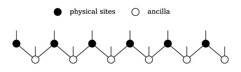
Figure 1: Structure of the matrix product states used in the purification approach of the finite temperature density matrix renormalization group algorithm.

In addition to the examples mentioned above, there exist several other finite temperature algorithms. Minimally entangled typical thermal states (METTS) algorithm [32, 33] which will be mentioned in Chapter 5 is another fulfillment of finite temperature DMRG based on importance sampling. Compared to the purification approach, METTS requires a smaller bond dimension and the statistical error decreases as the temperature lowers. However, METTS has only been applied to spin systems, because the original formulation does not allow the variation of electron numbers and thus is limited to canonical ensemble. One could potentially adapt METTS for a grand canonical ensemble by sampling the electron numbers or introducing a set of initial states which do not preserve the electron numbers. Determinantal quantum Monte Carlo (DQMC) [34] and finite temperature auxiliary field quantum Monte Carlo (FT-AFQMC) [35, 36] are two other finite temperature algorithms based on importance sampling of Slater determinants. Both of the two QMC methods utilizes Hubbard-Stratonovich transformation to transform the many-body imaginary time evolution operator to single-particle operators expressed as free fermions coupled to auxiliary fields. AFQMC applies a constrained path to alleviate the sign problem, yet the computational cost is still non-negligible to reach low enough temperatures with large system sizes. The dynamical mean-field theory (DMFT) [37, 38] is an embedding method which maps a many-body lattice problem to a many-body local problem. Since DMFT evaluates the frequencies, it can be naturally extended to finite temperature calculations with a finite temperature impurity solver. As most embedding methods, DMFT results are affected by the finite size effect, and extrapolation to thermodynamic limit (TDL) is needed to remove the artifact from the finite impurity size. All the above numerical algorithms have their pros and cons, and one could make their choices based on the properties of the system and evaluate the results by careful benchmarking.

2 Summary of research

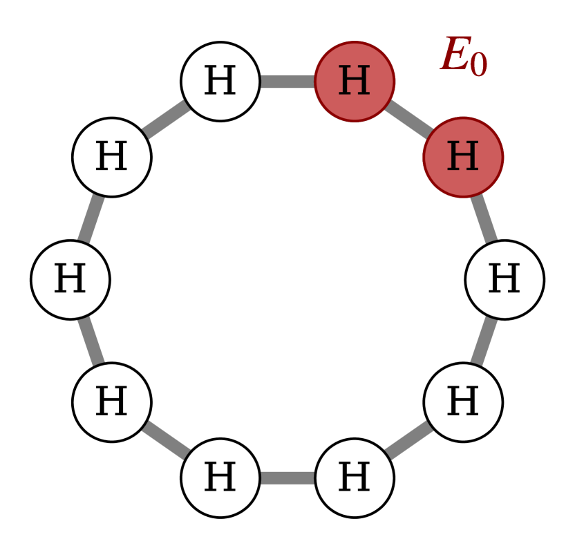
(a) $E_{\text{tot}}=5E_{0}$

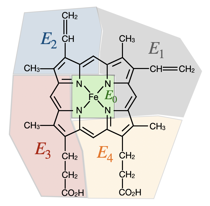
(b) $E_{\text{tot}}=\sum_{i=0}^{4}E_{i}$

Figure 2: Evaluating the total energy with density matrix embedding theory. (a) A hydrogen ring composed of $10$ atoms obeying the periodic boundary condition, and the impurity (supercell) is two adjacent atoms. The total energy equals the energy of the supercell times the number of supercells. (b) A single ligand heme molecule is divided into $5$ non-overlapping fragments, and the DMET energy of each fragment is calculated. The total energy is the sum of energies from all fragments.

This thesis provides several tools to study the finite temperature behaviors of strongly correlated materials. First we will introduce the finite temperature density matrix embedding theory (FT-DMET) in Chapter 2. FT-DMET, as a thermal extension of ground state DMET (GS-DMET) [39, 40, 41, 42], maps the many-body lattice thermal problem onto an impurity thermal problem. Same as in GS-DMET, the system is divided into non-overlapping fragments, which are defined by a set of local orbitals (LOs). For periodic systems, the fragments are chosen as supercells and thus all fragments are equivalent. For systems that do not obey periodicity, extensive observables are evaluated for each fragment and the total value of the observable is the summation of those from all fragments. An illustration is shown in Fig. 2 of the above two cases. Note that in the latter case, one should be careful when evaluating intensive properties, which should either be defined for a specific fragment or evaluated from global extensive properties. This real-space partition ensures that most of the entanglement is retained in the fragment for systems with short correlation lengths. When treating one fragment, we call this fragment the impurity and the rest of the fragments the environment.

To further capture the entanglement between the impurity and the environment, we introduce a term called bath. Bath in DMET is a subspace of the environment which is directly entangled with the impurity, spanned by a set of basis called bath orbitals. In strongly correlated systems, the correlation is highly localized, and the entanglement entropy obeys the area law. One could imagine that the bath orbitals mostly come from sites adjacent to the impurity. In practice, the bath orbitals are derived from the Schmidt decomposition of the total system wavefunction, which is initialized as the mean-field wavefunction and optimized in a bootstrap manner. A nice property of GS-DMET is that the number of bath orbitals generated from Schmidt decomposition is exactly equal to the number of impurity orbitals, with the assumption that the impurity is much smaller than the environment.

The key issue going from GS-DMET to FT-DMET is that the Schmidt decomposition no longer works since the system cannot be described by one single wavefunction. In fact the finite temperature state is described by a density matrix of the mixed state. Remember that the Schmidt decomposition of a wavefunction is equivalent to the singular value decomposition (SVD) of the corresponding density matrix. In FT-DMET algorithm, we start from the mean-field single-particle density matrix $\rho_{0}$, and apply SVD to the impurity-environment block to generate a set of bath orbitals, as described in the theory part in Chapter 2. Note that since the temperature enlarges the entanglement length, one should expect more bath orbitals to cover all impurity-environment entanglement than in GS-DMET. To do so, we continue to apply SVD to the impurity-environment block of powers of $\rho_{0}$ to get the rest of the bath orbitals. The algorithm is benchmarked with one- and two-dimensional Hubbard models, and shows systematically improved accuracy by increasing bath or impurity size.

In Chapter 3, we further extend the FT-DMET algorithm to handle ab initio problems. While model systems can be used to reproduce some of the behaviors and phases in realistic lattices, being able to perform ab initio simulations is key to achieve a complete understanding of the materials. There are two technical differences between model systems and ab initio systems: (ii) in most of the model systems, site basis is used which is naturally localized, while in ab initio systems the Coulomb interaction is of long range and the basis set used is usually not localized; (ii) in model systems, the two-body interaction form is very simple, while the two-body interaction in an ab initio Hamiltonian is described by a complicated rank-$4$ matrix. The above two technical difficulties are universal for all ab initio simulations. For ab initio FT-DMET, one also needs to deal with the large embedding space due to the size of the supercell and the basis set, which requires necessary truncation to the bath space. Moreover, a finite temperature impurity solver that can handle ab initio Hamiltonian efficiently is also crucial for any meaningful simulations. In Chapter 3, we provide solutions to the above problems and present the ab initio FT-DMET algorithm. We further use this algorithm to explore properties and phase transitions of hydrogen lattices.

Chapter 2 and Chapter 3 present an efficient numerical tool to simulate both strongly-correlated model systems and ab initio systems. The next question to answer is what order parameters we can use to capture essential thermal properties and phase transitions at finite temperature. In Chapter 4, we will study one of the most common but complex phase transitions: metal-insulator transition (MIT). We argue that compared to the band structure theory which is widely used to distinguish metal from insulator, electron locality is a more universal criteria which can be used to detect finite temperature MIT. We further introduce an order parameter named complex polarization to measure the locality of electrons and provide a thermofield approach to evaluate finite temperature complex polarization. The finite temperature complex polarization formulation provides an easy but well-defined way to characterize MIT in any periodic materials.

In Chapter 5, several quantum algorithms will be introduced for both ground state and finite temperature simulations on quantum devices. With the development of quantum computing technology, especially the hardware, it can be foreseen that certain categories of difficult problems in classical simulations can be solved with less effort on a quantum device. The bridge to connect chemical problems and successful quantum simulations is efficient quantum algorithms for noisy intermediate-scale quantum (NISQ) devices. Several quantum algorithms have been developed to carry out quantum chemical simulations in the past decades, including quantum phase estimation (QPE) [43, 44] and hybrid quantum-classical variational algorithms such as quantum approximate optimization algorithm (QAOA) [45, 46, 47] and variational quantum eigensolver (VQE) [48, 49, 50]. While the above algorithms have many advantages as advertised, they all require quantum or classical resources that can easily exceed the capacity of current devices. In Chapter 5, the key quantum algorithm that will be introduced is called quantum imaginary time evolution (QITE). As mentioned in Section 1, imaginary time evolution is an efficient algorithm to find the ground state. If the initial state is the identity density matrix at infinite temperature, then one could evaluate the density matrix and thus the thermal observables at any temperature.

The conflict of implementing imaginary time evolution on a quantum device is that the imaginary evolution operator $e^{\beta\hat{H}}$ is a non-unitary operator, while only unitary operators are allowed on a quantum device. We present an approach to reproduce a non-unitary operator with a rescaled unitary operation on an enlarged domain. This approach could be flexibly performed both exactly and approximately, depending on the computational resources available. The result is systematically improved and converges rapidly by increasing the size of the unitary domain. The convergence to the ground state can be further accelerated by the quantum Lanczos algorithm (QLanczos). QLanczos constructs a Krylov subspace with the intermediate states in QITE simulation, and then diagonalizes the Hamiltonian in the subspace representation to get a better approximation of the ground state. Unlike the classical Lanczos algorithm mentioned in Section 1 where the Krylov subspace is spanned by $\{|\psi_{0}\rangle,H|\psi_{0}\rangle,...,H^{m}|\psi_{0}\rangle\}$, the Krylov space in QLanczos is spanned by $\{|\psi_{0}\rangle,e^{2\tau\hat{H}}|\psi_{0}\rangle,...,e^{2m\tau\hat{H}}|\psi_{0}\rangle\}$. The Hamiltonian in the quantum Krylov space can be collected from the energy measurement at each step for free and no additional measurement is needed.

The third algorithm introduced in Chapter 5 is the quantum minimally entangled typical thermal states (QMETTS) algorithm. While the first two algorithms (QITE and QLanczos) can be applied to both ground state and finite temperature calculations, QMETTS is designed in particular for finite temperature simulations. QMETTS samples a set of minimally entangled thermal states under the thermal statistics by a repeated imaginary time evolving and then collapsing onto the product states routine. The advantage of the QMETTS algorithm is that the imaginary time evolution (fulfilled by QITE) always starts from a product state, so that the entanglement will not grow too large even at very low temperature. We present both classical and quantum simulations on a variety of problems using the above three quantum algorithms as examples and tests.

Chapter 2 Finite temperature density matrix embedding theory

3 Abstract

We describe a formulation of the density matrix embedding theory at finite temperature. We present a generalization of the ground-state bath orbital construction that embeds a mean-field finite-temperature density matrix up to a given order in the Hamiltonian, or the Hamiltonian up to a given order in the density matrix. We assess the performance of the finite-temperature density matrix embedding on the 1D Hubbard model both at half-filling and away from it, and the 2D Hubbard model at half-filling, comparing to exact data where available, as well as results from finite-temperature density matrix renormalization group, dynamical mean-field theory, and dynamical cluster approximations. The accuracy of finite-temperature density matrix embedding appears comparable to that of the ground-state theory, with at most a modest increase in bath size, and competitive with that of cluster dynamical mean-field theory.

4 Introduction

The numerical simulation of strongly correlated electrons is key to understanding the quantum phases that derive from electron interactions, ranging from the Mott transition [51, 52, 53, 54] to high temperature superconductivity [55, 56, 57]. Consequently, many numerical methods have been developed for this task. In the setting of quantum lattice models, quantum embedding methods [58], such as dynamical mean-field theory (DMFT)[59, 60, 61, 62, 63] and density matrix embedding theory (DMET)[39, 40, 42, 41, 64, 65, 66], have proven useful in obtaining insights into complicated quantum phase diagrams. These methods are based on an approximate mapping from the full interacting quantum lattice to a simpler self-consistent quantum impurity problem, consisting of a few sites of the original lattice coupled to an explicit or implicit bath. In this way, they avoid treating an interacting quantum many-body problem in the thermodynamic limit.

The current work is concerned with the extension of DMET to finite temperatures. DMET so far has mainly been applied in its ground-state formulation (GS-DMET), where it has achieved some success, particularly in applications to quantum phases where the order is associated with large unit cells [41, 64, 67]. The ability to treat large unit cells at relatively low cost compared to other quantum embedding methods is due to the computational formulation of DMET, which is based on modeling the ground-state impurity density matrix, a time-independent quantity accessible to a wide variety of efficient quantum many-body methods. Our formulation of finite-temperature DMET (FT-DMET) is based on the simple structure of GS-DMET, but includes the possibility to generalize the bath so as to better capture the finite-temperature impurity density matrix. Bath generalizations have previously been used to extend GS-DMET to the calculation of spectral functions and other dynamical quantities [68, 69]. Analogously to GS-DMET, since one only needs to compute time-independent observables, finite-temperature DMET can be paired with the wide variety of quantum impurity solvers which can provide the finite-temperature density matrix.

We describe the theory of FT-DMET in Section 5. In Section 6 we carry out numerical calculations on the 1D and 2D Hubbard models, using exact diagonalization (ED) and the finite-temperature density matrix renormalization group (FT-DMRG) [70] as quantum impurity solvers. We benchmark our results against those from the Bethe ansatz in 1D, and DMFT and the dynamical cluster approximation (DCA) in 2D, and also explore the quantum impurity derived Néel transition in the 2D Hubbard model. We finish with brief conclusions about prospects for the method in 7.

5 Theory

5.1 Ground state DMET

In this work, we exclusively discuss DMET in lattice models (rather than for ab initio simulations [42, 40, 66, 71]). As an example of a lattice Hamiltonian, and one that we will use in numerical simulations, we define the Hubbard model [72, 73],

$$\hat{H}=-t\sum_{\langle i,j\rangle,\sigma}\hat{a}^{\dagger}_{i\sigma}\hat{a}_{j\sigma}-\mu\sum_{i,\sigma}\hat{a}^{\dagger}_{i\sigma}\hat{a}_{i\sigma}+U\sum_{i}\hat{n}_{i\uparrow}\hat{n}_{i\downarrow}$$ (25)

where $\hat{a}^{\dagger}_{i\sigma}$ creates an electron with spin $\sigma$ on site $i$ and $\hat{a}_{i\sigma}$ annihilates it; $\hat{n}_{i\sigma}=\hat{a}^{\dagger}_{i\sigma}\hat{a}_{i\sigma}$; $t$ is the nearest-neighbour (denoted $\langle i,j\rangle$) hopping amplitude, here set to $1$; $\mu$ is a chemical potential; and $U$ is the on-site repulsion.

The general idea behind a quantum embedding method such as DMET is to approximately solve the interacting problem in the large lattice by dividing the lattice into small fragments or impurities [58]. (Here we will assume that the impurities are non-overlapping). The main question is how to treat the coupling and entanglement between the impurities. In DMET, other fragments around a given impurity are modeled by a set of bath orbitals. The bath orbitals are constructed to exactly reproduce the entanglement between the impurity and environment when the full lattice is treated at a mean-field level (the so-called “low-level” theory). The impurity together with its bath orbitals then constitutes a small embedded quantum impurity problem, which can be solved with a “high-level” many-body method. The low-level lattice wavefunction and the high-level embedded impurity wavefunction are made approximately consistent, by enforcing self-consistency of the single-particle density matrices of the impurities and of the lattice. This constraint is implemented by introducing a static correlation potential on the impurity sites into the low-level theory. The correlation potential introduced in DMET is analogous to the DMFT self-energy. A detailed discussion of the correlation potential including the comparison to other approaches such as density functional theory (DFT) can be found in  [58, 40].

To set the stage for the finite-temperature theory, in the following we briefly recapitulate some details of the above steps in the GS-DMET formulation. In particular, we discuss how to extract the bath orbitals, how to construct the embedding Hamiltonian, and how to carry out the self-consistency between the low-level and high-level methods. Additional details for the GS-DMET algorithm can be found in several articles  [39, 41, 42], including the review in Ref. [42].

5.1.1 DMET bath construction

Given a full lattice of $L$ sites, we define the impurity $x$ over $L_{x}$ sites, the Hilbert space of which is denoted as $\mathcal{A}^{x}$ and spanned by a set of orthonormal basis $\{|A^{x}_{i}\rangle\}$. The rest of the lattice is treated as the environment of impurity $x$, the Hilbert space of which is denoted as $\mathcal{E}^{x}$ spanned by an orthonormal basis $\{|E^{x}_{i}\rangle\}$. The Hilbert space of the entire lattice $\mathcal{H}$ is the direct product of the two subsystem Hilbert spaces: $\mathcal{H}=\mathcal{A}^{x}\otimes\mathcal{E}^{x}$. Any state $|\Psi\rangle$ in $\mathcal{H}$ can be written as

$$|\Psi\rangle=\sum_{ij}\psi_{ij}|A^{x}_{i}\rangle|E^{x}_{j}\rangle,$$ (26)

where the coefficients $\psi_{ij}$ form a $2^{n_{A}}\times 2^{n_{E}}$ matrix. Absorbing $\psi_{ij}$ into the environment orbitals, one could rewrite Eq. (26) as

$$\begin{split}|\Psi\rangle&=\sum_{i}|A^{x}_{i}\rangle\left(\sum_{j}\psi_{ij}|E^{x}_{j}\rangle\right)\\ &=\sum_{i}|A^{x}_{i}\rangle|B^{x}_{i}\rangle\end{split},$$ (27)

where $|B^{x}_{i}\rangle=\sum_{j}\psi_{ij}|E^{x}_{j}\rangle$. Eq. (27) tells us that the orbitals in $\mathcal{E}^{x}$ that are entangled to the impurity $x$ are of the same size as the impurity orbitals. Note that $\{|B^{x}_{i}\rangle\}$ are not orthonormal and the rest of the environment enters as a separatable product state $|\Psi_{\text{core}}\rangle$ called "core contribution". Let $\{|\tilde{B}^{x}_{i}\rangle\}$ denote the orthonormal states derived from $\{|B^{x}_{i}\rangle\}$, then Eq. (27) can be rewritten as

$$|\Psi\rangle=\left(\sum_{i}\lambda_{i}|A^{x}_{i}\rangle|\tilde{B}^{x}_{i}\rangle\right)|\Psi_{\text{core}}\rangle.$$ (28)

The orbitals $\{|\tilde{B}^{x}_{i}\rangle\}$ are directly entangled with the impurity $x$, and thus are called bath orbitals. The space spanned by impurity and bath is called embedding space. One can then derive the embedding state as

$$|\Psi_{\text{emb}}\rangle=\sum_{i}\lambda_{i}|A^{x}_{i}\rangle|\tilde{B}^{x}_{i}\rangle.$$ (29)

If $|\Psi\rangle$ is an eigenstate of the Hamiltonian $\hat{H}$ in the full lattice, then one can prove that $|\Psi_{\text{emb}}\rangle$ is also an eigenstate of the embedding Hamiltonian $\hat{H}_{\text{emb}}$ defined as the projection of $\hat{H}$ onto the embedding space. The two eigenvalues are identical. Therefore, the full lattice problem can be reduced to a smaller embedding problem.

In practice, the exact bath orbitals are unknown since the many-body eigenstate $|\Psi\rangle$ is the final target of the calculation. Instead, we construct a set of approximated bath orbitals from a mean-field ("low-level") wavefunction $|\Phi\rangle$, which is an eigenstate of a quadratic lattice Hamiltonian $\hat{h}$. We rewrite $|\Phi\rangle$ according to Eq. (28) and Eq. (29) in the form

$$|\Phi\rangle=|\Phi_{\text{emb}}\rangle|\Phi_{\text{core}}\rangle.$$ (30)

The single-particle density matrix $D^{\Phi}$ obtained from $|\Phi\rangle$ contains all information on the correlations in $|\Phi\rangle$. Thus the bath orbitals can be defined from this density matrix.

We consider the impurity-environment block $D^{\Phi}_{\text{imp-env}}$ ($D_{ij}$ for $i\in x,j\notin x$) of dimension $L^{x}\times(L-L^{x})$. Then taking the thin SVD

$$D^{\Phi}_{\text{imp-env}}=U\lambda B^{\dagger},$$ (31)

the columns of $B$ specify the bath orbitals in the lattice basis. The bath space is thus a function of the density matrix, denoted $B(D)$.

5.1.2 Embedding Hamiltonian

After obtaining the bath orbitals, we construct the embedded Hamiltonian of the quantum impurity problem. In GS-DMET, there are two ways to do so: the interacting bath formulation and the non-interacting bath formulation. The conceptually simplest approach is the interacting bath formulation. In this case, we project the interacting lattice Hamiltonian $\hat{H}$ into the space of the impurity plus bath orbitals, defined by the projector $\hat{P}$, i.e. the embedded Hamiltonian is $\hat{H}_{\text{emb}}=\hat{P}\hat{H}\hat{P}$. $\hat{H}_{\text{emb}}$ in general contains non-local interactions involving the bath orbitals, as they are non-local orbitals in the environment. From the embedded Hamiltonian, we compute the high-level ground-state impurity wavefunction,

$$\hat{H}_{\text{emb}}|\Psi\rangle=E|\Psi\rangle.$$ (32)

If $\hat{H}$ were itself the quadratic lattice Hamiltonian $\hat{h}$, then then $\Psi=\Phi$ and

$$\hat{P}\hat{h}\hat{P}|\Phi\rangle=E|\Phi\rangle.$$ (33)

Another way to write Eq. (33) for a mean-field state is

$$[{P}{h}{P},{P}{D}^{\Phi}{P}]=0,$$ (34)

where $h$ denotes the single-particle Hamiltonian matrix and $P$ is the single-particle projector into the impurity and bath orbitals. These conditions imply that the lattice Hamiltonian and the embedded Hamiltonian $\hat{H}_{\text{emb}}$ share the same ground-state at the mean-field level, which is the basic approximation in GS-DMET.

In the alternative non-interacting bath formulation, interactions on the bath are approximated by a quadratic correlation potential (discussed below). This formulation retains the same exact embedding property as the interacting bath formulation for a quadratic Hamiltonian. In practice, both formulations give similar results in the Hubbard model [65, 74], and the choice between the two depends on the available impurity solvers; the interacting bath formulation generates non-local two-particle interactions in the bath that not all numerical implementations can handle. In this work, we use the interacting bath formulation in the 1D Hubbard model where an ED solver is used. In the 2D Hubbard model, we use the non-interacting bath formulation, where both ED and FT-DMRG solvers are used. This latter choice is because the cost of treating non-local interactions in FT-DMRG is relatively high (and we make the same choice with ED solvers to keep the results strictly comparable).

5.1.3 Self-consistency

To maintain self-consistency between the ground-state of the lattice mean-field $|\Phi\rangle$, and that of the interacting embedded Hamiltonian $|\Psi\rangle$, we introduce a quadratic correlation potential $\hat{u}$ into $h$, i.e.

$$\hat{h}\to\hat{h}+\hat{u},$$ (35)

where $\hat{u}$ is constrained to act on sites in the impurities, i.e. $\hat{u}=\sum_{x}\hat{u}^{x}$. To study magnetic order, we choose the form

$$\hat{u}^{x}=\sum_{ij\in x,\sigma\in\{\uparrow,\downarrow\}}u^{x}_{ij\sigma}a^{\dagger}_{i\sigma}a_{j\sigma}.$$ (36)

The coefficients $u^{x}_{ij\sigma}$ are adjusted to match the density matrices on the impurity that are evaluated from the low-level wavefunction $|\Phi\rangle$ and from the high-level embedded wavefunction $|\Psi\rangle$. In this work, we only match the single-particle density matrix elements of the impurity (impurity-only matching [42]) by minimizing the cost function:

$$f(u)=\sum_{i,j\in\text{imp}}(D_{ij}^{\text{low}}-D_{ij}^{\text{high}})^{2},$$ (37)

where $D^{\text{low}}$ and $D^{\text{high}}$ are single-particle density matrices of low-level and high-level solutions, respectively. For each minimization iteration, we assume that the high-level single-particle density matrix is fixed, and the gradient of Eq. (37) is

$$\frac{\mathrm{d}f}{\mathrm{d}u}=\sum_{i,j\in\text{imp}}2(D_{ij}^{\text{low}}-D_{ij}^{\text{high}})\frac{\mathrm{d}D_{ij}^{\text{low}}}{\mathrm{d}u}.$$ (38)

For ground state, Ref. [42] provided an analytical approach to evaluate $\frac{\mathrm{d}D_{ij}^{\text{low}}}{\mathrm{d}u}$ using the first order perturbation theory. At finite temperature, one could also evaluate the gradient analytically as shown in the Appendix.

Note also that we will only be considering translationally invariant systems, and thus $\hat{u}^{x}$ is the same for all impurities.

5.2 Ground-state expectation values

Ground-state expectation values are evaluated from the density matrices of each high-level impurity wavefunctions $|\Psi^{x}\rangle$. Since there are multiple impurities (in a translationally invariant system, these are constrained to be identical), an expectation value is typically assembled from the multiple impurity wavefunctions using a democratic partitioning [42]. For example, given two sites $i$, $j$, where $i$ is part of impurity $x$ and $j$ is part of impurity $y$, the expectation value of $a^{\dagger}_{i}a_{j}$ is

$$\langle a^{\dagger}_{i}a_{j}\rangle=\frac{1}{2}[\langle\Psi^{x}|a^{\dagger}_{i}a_{j}|\Psi^{x}\rangle+\langle\Psi^{y}|a^{\dagger}_{i}a_{j}|\Psi^{y}\rangle].$$ (39)

Note that the pure bath components of the high-level wavefunctions, e.g. $\langle\Psi^{x}|a^{\dagger}_{i}a_{j}|\Psi^{x}\rangle$ for $i,j\notin x$ are not used in defining the DMET expectation values. Instead, the democratic partitioning is arranged such that an individual impurity embedding contributes the correct amount to a global expectation value so long as the impurity wavefunction produces correct expectation values for operators that act on the impurity alone, or the impurity and bath together.

5.3 Finite temperature DMET

Our formulation of FT-DMET follows the same rubric as the ground-state theory: a low-level (mean-field-like) finite-temperature density matrix is defined for the lattice; this is used to obtain a set of bath orbitals to define the impurity problem; a high-level finite-temperature density matrix is calculated for the embedded impurity; and self-consistency is carried out between the two via a correlation potential. The primary difference lies in the properties of the bath, which we focus on below, as well as in the appearance of quantities such as the entropy, which are formally defined from many-particle expectation values.

5.3.1 Finite temperature bath construction

In GS-DMET bath construction, the bath orbitals are directly defined from Schmidt decomposition of the full lattice ground state wavefunction as in Eq. (28). However, at finite temperature, the state of an open quantum system (grand canonical ensemble) is described by a mixed state: the density matrix is described by a linear combination of pure state density matrices. As a consequence, the Schmidt decomposition can no longer be used to define bath orbitals. In fact, with non-zero temperature, the entanglement becomes more delocalized. To capture the entanglement between the impurity and environment, a larger bath space is needed compared to that of ground state. In Fig. 3, we plotted the weight of entanglement with the impurity as a function of distance (in sites) from the impurity for a $100$-site tight binding model ($\hat{H}=\sum_{i}\hat{a}_{i}^{\dagger}\hat{a}_{i+1}+\text{h.c.}$). One could see that as the temperature rises, more and more farther sites are entangled with the impurity, and eventually all sites are uniformly and maximumly entangled. At ground state ($T=0$), the weight decreased with distance with an oscillating manner, with wavelength = $2$ sites; at $T=0.15$, the wavelength increased to $6$ sites due to the smearing effect of finite temperature. The increase of oscillating wavelength is another example of the increase of correlation length with temperature.

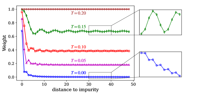
Figure 3: Weight of the entanglement with the impurity on environmental sites. The weights are evaluated as the square norm of projections of environmental sites to the bath space. Due to periodicity of the system, only half of the environmental sites are shown in the figure.

The difficulty of finite temperature bath orbital construction can also be demonstrated by the commutation relation between the projected single-particle density matrix and projected Hamiltonian. In GS-DMET, the bath orbital construction is designed to be exact if all interactions are treated at the mean-field level, giving rise to the commuting condition for the projected single-particle density matrix and projected Hamiltonian in Eq. (34). At finite temperature, the above commuting condition does not stand and one should expect approximated bath orbitals even at mean-field level. In general, we can look for a finite-temperature bath construction that preserves a similar property. As pointed out in Sec. 5.2, the DMET embedding is still exact for single-particle expectation values if the embedded projected single-particle density matrix produces the correct expectation values in the impurity and impurity-bath sectors, due to the use of the democratic partitioning. We aim to satisfy this slightly relaxed condition.

The finite temperature single-particle density matrix of a quadratic Hamiltonian $\hat{h}$ is given by the Fermi-Dirac function

$${D}(\beta)=\frac{1}{1+e^{({h}-\mu)\beta}},$$ (40)

where $\beta=1/k_{B}T$ ($k_{B}$ is the Boltzmann constant, $T$ is the temperature). In the following, we fix $k_{B}=1$, thus $\beta=1/T$. If we could find an embedding directly analogous to the ground-state construction, we would obtain a projector ${P}$, such that the embedded density matrix ${P}{D}{P}$ is the Fermi-Dirac function of the embedded quadratic Hamiltonian, i.e. ${P}h{P}$, i.e.

$${P}{D}{P}=\frac{1}{1+e^{({P}{h}{P}-\mu)\beta}}.$$ (41)

However, unlike in the ground-state theory, the non-linearity of the exponential function means that Eq. (41) can only be satisfied exactly if ${P}$ projects back into the full lattice basis. Thus a bath orbital construction at finite temperature is necessarily always approximate, even for quadratic Hamiltonians.

Nonetheless, one can choose the bath orbitals to reduce the error between the l.h.s. and r.h.s. in Eq. (41). First, we require that the equality is satisfied only for the impurity-environment block of $D$, following the relaxed requirements of the democratic partitioning. Second, we require the equality to be satisfied only up to a finite order $n$ in $h$, i.e.

$$[PDP]_{ij}=\left[\frac{1}{1+e^{({P}{h}{P}-\mu)\beta}}\right]_{ij}+O(h^{n})\quad i\in x,j\notin x.$$ (42)

Then there is a simple algebraic construction of the bath space as (see Appendix for a proof)

$$\{B(h)\oplus B(h^{2})\oplus B(h^{3})\ldots B(h^{n})\},$$ (43)

where $B(h^{k})$ is the bath space derived from $h^{k}$, $k=1,...,n$. Note that each order of $h$ adds $L_{x}$ bath orbitals to the total impurity plus bath space.

We can alternatively choose the bath to preserve the inverse relationship between the density matrix and Hamiltonian,

$$[PhP]_{ij}=\mathrm{inverseFD}(PDP)+O(D^{n})\quad\mathrm{not}\ i,j\notin x,$$ (44)

where $\mathrm{inverseFD}$ is the inverse Fermi-Dirac function, and the bath space is then given as

$$\{B(D)\oplus B(D^{2})\oplus B(D^{3})\ldots B(D^{n})\}.$$ (45)

The attraction of this construction is that the lowest order corresponds to the standard GS-DMET bath construction.

The above generalized bath constructions allow for the introduction of an unlimited number of bath sites (so long as the total number of sites in the embedded problem is less than the lattice size). Increasing the size of the embedded problem by increasing the number of bath orbitals (hopefully) increases the accuracy of the embedding, but it also increases the computational cost. However, an alternative way to increase accuracy is simply to increase the number of impurity sites. Which strategy is better is problem dependent, and we will assess both in our numerical experiments.

5.3.2 Thermal observables

The thermal expectation value of an observable $\hat{O}$ is defined as

$$\langle\hat{O}(\beta)\rangle=\Tr\left[\hat{\rho}(\beta)\hat{O}\right].$$ (46)

Once $\hat{\rho}(\beta)$ is obtained from the high-level impurity calculation, for observables based on low-rank (e.g. one- and two-) particle reduced density matrices, we evaluate Eq. (46) using the democratic partitioning formula for expectation values in Sec. 5.2.

We will also, however, be interested in the entropy per site, which is a many-particle expectation value. Rather than computing this directly as an expectation value, we will obtain it by using the thermodynamic relation $\frac{\dd S}{\dd E}=\beta$, and

$$S(\beta_{0})=S(0)+\int_{E(0)}^{E(\beta_{0})}\beta(E)\dd E$$ (47)

where $\beta_{0}$ is the desired inverse temperature, and $S(0)=\ln 4\approx 1.386$.

6 Results

6.1 Computational details

We benchmarked the performance of FT-DMET in the 1D and 2D Hubbard models as a function of $U$ and $\beta$. For the 1D Hubbard model, we compared our FT-DMET results to exact solutions from the thermal Bethe ansatz  [75]. For the 2D Hubbard model, the FT-DMET results were compared to DCA and DMFT results [76, 2, 1, 3, 4, 77]. We used large DMET mean-field lattices with periodic boundary conditions (240 sites in 1D, $24\times 24$ sites in 2D). We used exact diagonalization (ED) and finite temperature DMRG (FT-DMRG) as impurity solvers. There are two common ways to carry out FT-DMRG calculations: the purification method [70] and the minimally entangled typical thermal states (METTS) method [78]. In this work, we used the purification method implemented with the ITensor package [79] as the FT-DMRG impurity solver, as well as to provide the finite lattice reference data in Fig.8. In the FT-DMRG solver, the sites were ordered with the impurity sites coming first, followed by the bath sites (an orthonormal basis for the set of bath sites of different orders was constructed via singular value decomposition, and ordered in decreasing size of the singular values) and the ancillae arranged in between each physical site. In the 1D Hubbard model, we used ED exclusively and the interacting bath formulation of DMET, while in the 2D Hubbard model, we used ED for the 4 impurity, 4 bath calculations, and FT-DMRG for the 4 impurity, 8 bath calculations, both within the non-interacting bath formulation. FT-DMRG was carried out using 4th order Runge-Kutta time evolution. To denote different calculations with different numbers of impurity and bath orbitals, we use the notation $InBm$, where $n$ denotes the number of impurity sites and $m$ the number of bath orbitals.

6.2 1D Hubbard model

The 1D Hubbard model is an ideal test system for FT-DMET as its thermal properties can be exactly computed via the thermal Bethe ansatz. We thus use it to assess various choices within the FT-DMET formalism outlined above.

We first compare the relative performance of the two proposed bath constructions, generated via the Hamiltonian in Eq. (43) or via the density matrix in Eq. (45). In Fig. 4, we show the error in the energy per site (measured from the thermal Bethe ansatz) for $U=2,4$ and half-filling for these two choices. (The behaviour for other $U$ is similar). Using 4 bath sites, the absolute error in the energy is comparable to that of the ground-state calculation (which uses 2 bath sites) over the entire temperature range. Although the Hamiltonian construction was motivated by the high temperature expansion of the density matrix, the density matrix construction appears to perform well at both low and high temperatures. Consequently, we use the density matrix derived bath in the subsequent calculations.

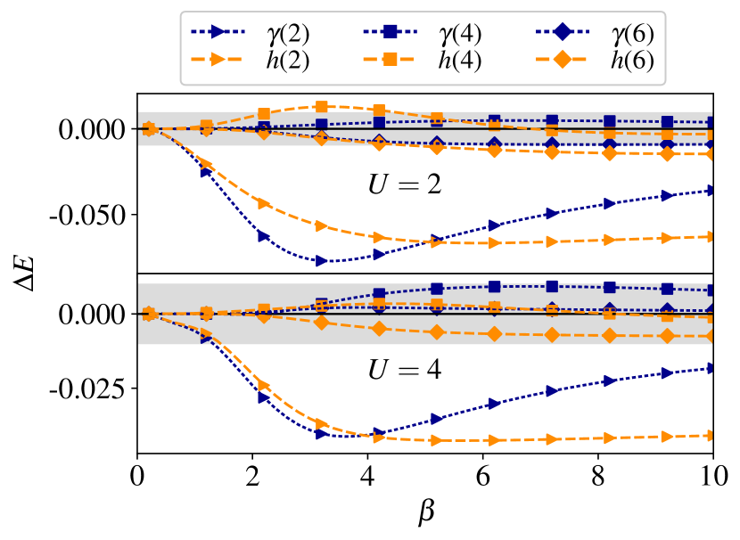
Figure 4: Error in energy per site (units of $t$) of FT-DMET for the 1D Hubbard model at $U=2$ and $U=4$ (2 impurity sites and half-filling) with bath orbitals generated via the density matrix $\gamma$ (Eq. (45)) (blue lines) or lattice Hamiltonian $h$ (Eq. (43)) (orange lines) as a function of inverse temperature $\beta$. The numbers in parentheses denote the number of bath orbitals. The grey area denotes the ground state error with 2 impurity orbitals.

We next examine the effectiveness of the density matrix bath construction in removing the finite size error of the impurity. As a first test, in Fig. 5 we compare the energy error obtained with FT-DMET and $I2B2$ with a pure ED calculation with 4 impurity sites ($I4$) and periodic (PBC) or antiperiodic (APBC) boundary conditions, at various $U$ and $\beta$. For weak ($U=2$) to moderate ($U=4$) coupling, FT-DMET shows a significant improvement over a finite system calculation with the same number of sites, reducing the error by a factor of $\sim 2-6$ depending on the $\beta$, thus demonstrating the effectiveness of the bath. The maximum FT-DMET energy error is 8.1, 6.6, 3.1% for $U=2,4,8$. At very strong couplings, the error of the finite system ED with PBC approaches that of FT-DMET. This is because both the finite size error and the effectiveness of the DMET bath decrease as one approaches the atomic limit.

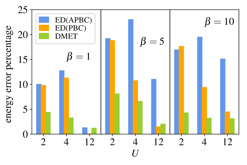
Figure 5: Percentage error of the FT-DMET (with 2 impurity sites and 2 bath orbitals) energy per site vs. ED (4 sites) on a non-embedded cluster with PBC and APBC boundary conditions for the 1D Hubbard model at various $U$ and $\beta$.

As a second test, in Fig. 6 we compare increasing the number of impurity sites versus increasing the number of bath orbitals generated in Eq. (45) for various $U$ and $\beta$. Although complex behaviour is seen as a function of $\beta$, we roughly see two patterns. For certain impurity sizes, (e.g. $I4$) it can be slightly more accurate to use a larger impurity with an equal number of bath sites, than a smaller impurity with a larger number of bath sites. (For example, at $U=8$, one can find a range of $\beta$ where $I4B4$ gives a smaller error than $I2B6$). However, there are also some impurity sizes which perform very badly; for example $I3B3$ gives a very large error, because the (short-range) antiferromagnetic correlations do not properly tile between adjacent impurities when the impurities are of odd size. Thus, due to these size effects, convergence with impurity size is highly non-monotonic, but increasing the bath size (by including more terms in Eq. (45)) is less prone to strong odd-size effects. The ability to improve the quantum impurity by simply increasing the number of bath sites, is expected to be particularly relevant in higher-dimensional lattices such as the 2D Hubbard model, where ordinarily to obtain a sequence of clusters with related shapes, it is necessary to increase the impurity size by large steps. Nonetheless, convergence with bath size is also not strictly monotonic, as also illustrated in Fig. 7, where we see that the error in the $I2B4$ entropy can sometimes be less than that of $I2B6$ for certain ranges of $\beta$. For the largest embedded problem $I2B6$, the maximum error in the entropy is $4\times 10^{-3}$ and $2\times 10^{-2}$ for $U=4$ and $8$, respectively.

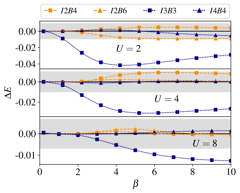
Figure 6: Absolute error of the FT-DMET energy per site of the 1D Hubbard model at half-filling as a function of impurity and bath size. $InBm$ denotes $n$ impurity sites and $m$ bath orbitals. Increasing impurity (blue lines); increasing bath (orange lines). The grey band depicts the ground state error with $2$ impurity sites and $2$ bath orbitals.

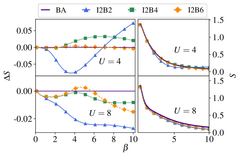
Figure 7: Absolute error of the FT-DMET entropy per site of the 1D Hubbard model at half-filling as a function of the number of bath sites. The right panels show the absolute entropy.

The preceding calculations were all carried out at half-filling. Thus, in Fig. 8 we show FT-DMET calculations on the 1D Hubbard model away from half-filling at $U=4$. We chose to simulate a finite Hubbard chain of 16-sites with PBC in order to readily generate numerically exact reference data using FT-DMRG (using a maximum bond dimension of $2000$ and an imaginary time step of $\tau=0.025$). The agreement between the FT-DMRG energy per site and that obtained from the thermal Bethe ansatz can be seen at half-filling, corresponding to a chemical potential $\mu=2$. We see excellent agreement between FT-DMET and FT-DMRG results across the full range of chemical potentials, and different $\beta$, suggesting that FT-DMET works equally well for doped systems as well as for undoped systems.

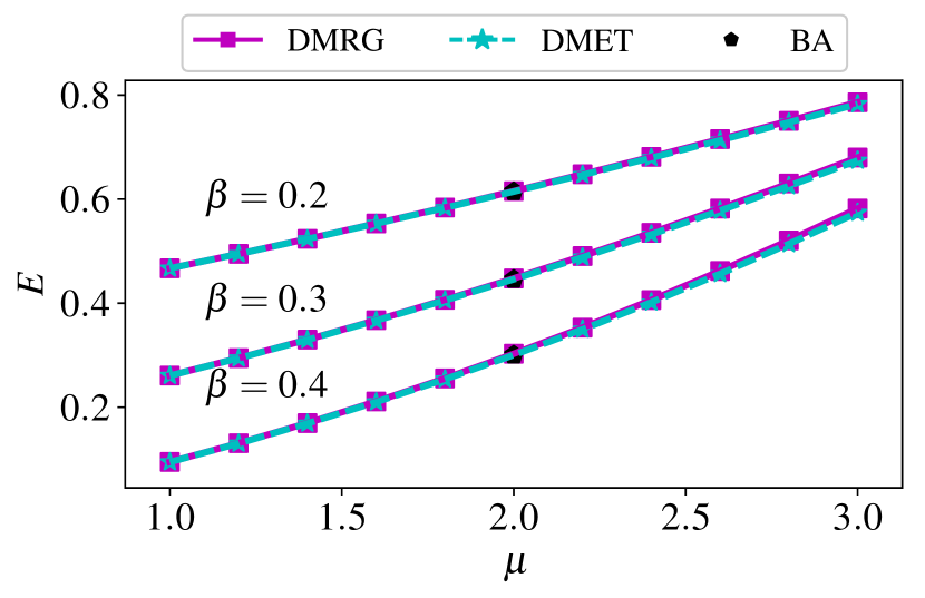
Figure 8: Energy per site (units of $t$) of a 16-site Hubbard chain with periodic boundary conditions at $U=4$ as a function of the chemical potential $\mu$ at various $\beta$ values. The difference between the DMRG and DMET ($I2B6$) energies per site is $0.01-1.4\%$. Solid lines: DMRG energies; dashed lines: DMET energies; pentagons: Bethe ansatz.

6.3 2D Hubbard model

The 2D Hubbard model is an essential model of correlation physics in materials. We first discuss the accuracy of FT-DMET for the energy of the 2D Hubbard model at half-filling, shown in Fig. 9. The FT-DMET calculations are performed on a $2\times 2$ impurity, with 4 bath orbitals ($I4B4$) (green diamond markers) and 8 bath orbitals ($I4B8$) (red triangular markers). The results are compared to DCA calculations with clusters of size $34$ (orange circle markers), $72$ (blue square markers) [77], and $2\times 2$ (light blue hexagon markers) (computed for this work). The DCA results with the size $72$ cluster can be considered here to represent the thermodynamic limit. The DCA($2\times 2$) data provides an opportunity to assess the relative contribution of the FT-DMET embedding to the finite size error; in particular, one can compare the difference between FT-DMET and DCA(72) to the difference between DCA($2\times 2$) and DCA(72). Overall, we see that the FT-DMET energies with 8 bath orbitals are in good agreement with the DCA(72) energies across the different $U$ values, and that the accuracy is slightly better on average than that of DCA($2\times 2$). The maximum error in the $I4B8$ impurity compared to thermodynamic limit extrapolations of the DCA energy [77] is found at $U=4$ and is in the range of 1-2%, comparable to errors observed in ground-state DMET at this cluster size (e.g. the error in GS-DMET at $U=4$ and $U=8$ is 0.3% and 1.8%, respectively). In the $\beta=8$ case, the FT-DMET calculations with two different bath sizes give very similar results; at low temperature, the bath space constructed by the FT procedure is similar to that of the ground state, and the higher order bath sites do not contribute very relevant degrees of freedom. Thus even the smaller bath achieves good accuracy in the low temperature FT-DMET calculations.

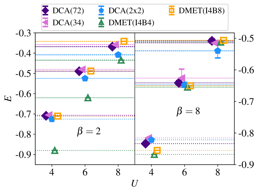
Figure 9: Energy per site versus U (units of $t$) of the 2D Hubbard model at half-filling with FT-DMET ($2\times 2$ cluster with 4 and 8 bath orbitals), DCA (34, 72 and $2\times 2$ site clusters).

(a)

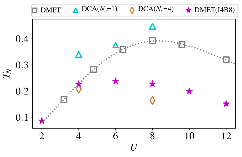
(b)

Figure 10: Néel transition for the 2D Hubbard model within quantum impurity simulations. (a) Antiferromagnetic moment $m$ as a function of $T$ with various $U$ values (units of $t$); (b) Néel temperature $T_{N}$ calculated with FT-DMET, single-site DMFT and DCA. DMFT data is taken from Ref. [1], DCA/NCA data for $U=4$ is taken from Ref. [2], DCA/QMC data for $U=6$ is taken from Ref. [3], and DCA/QMC data for $U=8$ is taken from Ref. [4].

A central phenomenon in magnetism is the finite-temperature Néel transition. In the thermodynamic limit, the 2D Hubbard model does not exhibit a true Néel transition, but shows a crossover [80]. However, in finite quantum impurity calculations, the crossover appears as a phase transition at a nonzero Néel temperature. Fig. 10(a) shows the antiferromagnetic moment $m$ calculated as $m=\frac{1}{2L_{x}}\sum_{i}^{L_{x}}|n_{i\uparrow}-n_{i\downarrow}|$ as a function of temperature $T$ for various $U$ values. As a guide to the eye, we fit the data to a mean-field magnetization function $m=a\tanh\left(bm/T\right)$, where $a$ and $b$ are parameters that depend on $U$. The FT-DMET calculations are performed with a $2\times 2$ impurity and $8$ bath orbitals, using a finite temperature DMRG solver with maximal bond dimension $M=600$ and time step $\tau=0.1$. With this, the error in $m$ from the solver is estimated to be less than 10^-3. $m$ drops sharply to zero as $T$ is increased signaling a Néel transition. The Néel temperature $T_{N}$ is taken as the point of intersection of the mean-field fitted line with the $x$ axis; assuming this form of the curve, the uncertainty in $T_{N}$ is invisible on the scale of the plot. The plot of $T_{N}$ versus $U$ is shown in Fig. 10(b), showing that the maximal $T_{N}$ occurs at $U=6$. Similar $T_{N}$ calculations on the 2D Hubbard model with single site DMFT [1] and DCA[3, 4, 2] are also shown in Fig. 10(b) for reference. Note that the difference in the DMFT results [1] and single-site DCA (formally equivalent to DMFT) [3, 4] likely arise from the different solvers used. The behaviour of $T_{N}$ in our $2\times 2$ FT-DMET calculations is quite similar to that of the 4-site DCA cluster. In particular, we see in DCA that the $T_{N}$ values obtained from calculations with a single-site cluster ($N_{c}=1$) are higher than the $T_{N}$ values obtained from calculations with a 4-site cluster ($N_{c}=4$).

An alternative visualization of the Néel transition in FT-DMET is shown in Fig. 11. The FT-DMET calculations here were performed with a $2\times 2$ impurity and $4$ bath orbitals using an ED solver. Though less quantitatively accurate than the $8$ bath orbital simulations, these FT-DMET calculations still capture the qualitative behavior of the Néel transition. Focusing on the dark blue region of the phase diagram, one can estimate the maximal $T_{N}$ to occur near $U\approx 9$, an increase over the maximal Néel temperature using the $8$ bath orbital impurity model. This increase in the maximal $T_{N}$ appears similar to that which happens when moving from a 4-site cluster to a 1-site cluster in DCA in Fig. 10.

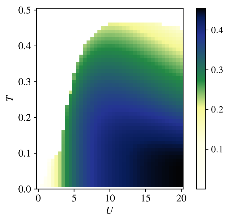
Figure 11: 2D Hubbard antiferromagnetic moment (color scale) as a function of $T$ and $U$ (units of $t$) in FT-DMET ($2\times 2$ impurity, 4 bath orbitals.)

7 Conclusions

To summarize, we have introduced a finite temperature formulation of the density matrix embedding theory (FT-DMET). This temperature formulation inherits most of the basic structure of the ground-state density matrix embedding theory, but modifies the bath construction so as to approximately reproduce the mean-field finite-temperature density matrix. From numerical assessments on the 1D and 2D Hubbard model, we conclude that the accuracy of FT-DMET is comparable to that of its ground-state counterpart, with at most a modest increase in size of the embedded problem. From the limited comparisons, it also appears to be competitive in accuracy with the cluster dynamical mean-field theory for the same sized cluster. Similarly to ground-state DMET, we expect FT-DMET to be broadly applicable to a wide range of model and ab initio problems of correlated electrons at finite temperature [64, 71].

Chapter 3 Ab initio finite temperature density matrix embedding theory

8 Abstract

This work describes the framework of the finite temperature density matrix embedding theory (FT-DMET) for ab initio simulations of solids. We introduce the implementation details including orbital localization, density fitting treatment to the two electron repulsion integrals, bath truncation, lattice-to-embedding projection, and impurity solvers. We apply this method to study the thermal properties and phases of hydrogen lattices. We provide the finite temperature dissociation curve, paramagnetic-antiferromagnetic transition, and metal-insulator transition of the hydrogen chain.

9 Introduction

The numerical study of the many-electron problem has been playing a profound role in understanding the electronic behaviors in molecules and materials. One big challenge for current numerical methods is the description of strong electron correlations, which requires non-trivial treatment of the electron-electron interaction beyond the mean-field level. A variety of numerical algorithms have been invented in the past decades to treat strong electron correlations, including post-Hartree-Fock quantum chemistry methods such as CCSD [81, 82], DMRG and its multi-dimensional alternatives [83, 84, 85, 86, 87], the QMC family such as AFQMC [88, 89, 23], and embedding methods such as DMET [90, 91]. During the past decades, noticeable progress has been made in the study of strongly correlated models such as one-dimensional and two-dimensional Hubbard models[92, 93, 94], while the ab initio study of strongly correlated solids is rare. Compared to model systems where forms of the two-electron interaction are usually simple, ab initio Hamiltonians contain much more complicated two-electron terms with size $N^{4}$, where $N$ is the number of orbitals. This complexity brings higher computational costs. Therefore, an efficient method that can handle the realistic Hamiltonian accurately is crucial for understanding the physics behind real materials.

The hydrogen lattice is believed to be the simplest chemical system with a straightforward analog to the Hubbard model. A thorough comparison between the hydrogen lattice and Hubbard model could provide insights of the roles of (i) the long range correlation and (ii) the multi-band effect (with basis set larger than STO-6G). The numerical study of hydrogen chain can be traced back to the 70s with simple theoretical tools such as many body perturbation theory (MBPT)[95]. The rapid development of numerical algorithms made it possible to achieve a better accuracy and thus plausible conclusions[96, 97, 98, 99, 100, 101, 102, 5]. Motta et al. benchmarked the equation of state[101] and explored the ground state properties[102] of the hydrogen chain with various popular numerical methods including DMRG and AFQMC. Despite the numerous ground state simulations, the finite temperature study of hydrogen lattices is rare, while the finite temperature study is crucial for understanding the temperature-related phase diagrams. Liu et. al. studied the finite temperature behaviors of hydrogen chain with the minimal basis set (STO-6G), and identified the signature of Pomeranchuk effect[5]. However, the minimal basis set hindered the exploration of more interesting phenomena caused by the multi-band effect. A more thorough study beyond the minimal basis set is needed to reach a quantitative observation of the finite temperature behaviors of the hydrogen lattices.

In this work, we apply ab initio finite temperature density matrix embedding theory (FT-DMET) [103] algorithm to study metal-insulator and magnetic crossovers in periodic one-dimensional and two-dimensional hydrogen lattices as a function of temperature $T$ and H-H bond distance $R$. We also explore how basis set size influences the shape of the phases by comparing the results with STO-6G, 6-31G, and CC-PVDZ basis sets. The rest of the article is organized as follows: in Section 10, we present the formulation and implementation details of ab initio FT-DMET, including orbital localization, tricks to reduce the cost due to the two electron repulsion terms, bath truncation, impurity solver, and thermal observables. In Section 11, we demonstrate the ab initio FT-DMET algorithm by studies of the dissociation curves and phase transitions in a one-dimensional periodic hydrogen lattice. We finalize this article with conclusions in Section 12.

10 Ab initio FT-DMET

In our previous work[103], we introduced the basic formulation of FT-DMET for lattice models. Going from lattice models to chemical systems, there are several practical difficulties[104]: (i) the definition of impurity relies on the localization of the orbitals; (ii) the number of orbitals in the impurity can be easily very large depending on the infrastructure of the supercell and the basis set; (iii) manipulating two-electron repulsion integrals in a realistic Hamiltonian is usually very expensive; (iv) an impurity solver which can handle ab initio Hamiltonians efficiently at finite temperature is required. In the rest of this section, we discuss solutions to the above challenges and provide implementation details of ab initio FT-DMET.

10.1 Orbital localization

Since we are dealing with periodic lattices, the whole lattice problem is described with Bloch (crystal) orbitals in the momentum space. Thus crystal atomic orbitals (AOs) $\{\phi^{\textbf{k}}_{\mu}(\textbf{r})\}$ are a natural choice. The definition of impurity, however, is based on real space localized orbitals [105]. Therefore we define a two-step transformation from Bloch orbitals to localized orbitals (LOs) $\{w_{i}(\mathbf{r})\}$.

$$\begin{split}w_{i}^{\mathbf{R}}(\mathbf{r})=&\frac{1}{\sqrt{N_{\mathbf{k}}}}\sum_{\mathbf{k}}e^{-i\mathbf{k}\cdot\mathbf{R}}w_{i}^{\mathbf{k}}(\mathbf{r}),\\ w_{i}^{\mathbf{k}}(\mathbf{r})=&\sum_{\mu}\phi^{\textbf{k}}_{\mu}(\textbf{r})C_{\mu i}^{\textbf{k}},\end{split}$$ (48)

where $C_{\mu i}^{\textbf{k}}$ transforms AOs in momentum space $\{\phi^{\textbf{k}}_{\mu}(\textbf{r})\}$ into LOs in momentum space $w_{i}^{\mathbf{k}}(\mathbf{r})$, and LOs in real space $w_{i}^{\mathbf{R}}(\mathbf{r})$ are derived by a Wannier summation over the local crystal orbitals $w_{i}^{\mathbf{k}}(\mathbf{r})$.

With the ab initio periodic system expressed in LOs, one could choose the impurity to be spanned by the LOs in a single unit cell or supercell. In the rest of this paper, we choose the impurity to be the supercell at the lattice origin.

To define the localization coefficients $C_{\mu i}^{\textbf{k}}$ in Eq. (48), we use a bottom-up strategy: transform from AO computational basis to LOs. This strategy uses linear algebra to produce LOs, and thus avoids dealing with complicated optimizations. There are several choices of LOs from the bottom-up strategy: Löwdin and meta-Löwdin orbitals [106], natural AOs (NAO) [107, 108], and intrinsic AOs (IAO) [40]. In this work, we used the $\mathbf{k}$-space unrestricted Hartree-Fock (KUHF) function with density fitting in the quantum chemistry package PySCF[109, 110] to generate a set of crystal MOs. Then we applied an adapted IAO routine to generate a set of crystal IAOs from the crystal MOs with $\mathbf{k}$-point sampling. The crystal IAOs generated from this routine are valence orbitals that exactly span the occupied space of the mean-field calculation. Note that the number of crystal IAOs is equal to the size of minimal basis only. To carry out calculations beyond the minimal basis, we construct the rest nonvalence orbitals to be projected AOs (PAOs) [111], orthogonalized with Löwdin orthogonalization [112]. This IAO+PAO strategy has been used in previous ground state DMET calculations [42, 104].

10.2 Bath truncation and finite temperature bath

In the standard DMET routine, the bath orbitals used to construct the embedding space are obtained from the SVD of the mean-field off-diagonal density matrix between the impurity and the remaining lattice (called environment) $\gamma^{\mathbf{R}\neq\mathbf{0},\mathbf{0}}$

$$\gamma^{\mathbf{R}\neq\mathbf{0},\mathbf{0}}=B^{\mathbf{R}\neq\mathbf{0}}\Lambda V^{\mathbf{0}{\dagger}},$$ (49)

where $B^{\mathbf{R}}$ defines the coefficients of bath orbitals in the LO basis. Thus we can construct the projection matrix in real space

$$P^{\mathbf{R}}=\begin{pmatrix}\mathbf{I}&\mathbf{0}\\ \mathbf{0}&\mathbf{B^{R\neq 0}}\end{pmatrix}.$$ (50)

The projection in momentum space can be derived from Eq. (50) with Wannier transformation

$$P^{\mathbf{k}}=\sum_{\mathbf{R}}e^{-i\mathbf{k\cdot R}}P^{\mathbf{R}}.$$ (51)

Note that the projection matrices $P^{\mathbf{R}}$ and $P^{\mathbf{k}}$ are in the basis of LOs, and to obtain the $\mathbf{k}$-space transformation matrix in AOs, simply multiply $C^{\mathbf{k}}$ from Eq. (48) to the left of $P^{\mathbf{k}}$.

From Eq. 49, one generates a set of bath orbitals with the same size as the impurity. This setting is valid and efficient for model systems, and the embedding space is purely constructed with valence bands. However, for ab inito calculations, low-lying core and high-energy virtual impurity orbitals will not entangle with the environment, and thus with the bath orbitals. In practice, this results in singular values in the SVD of Eq. (49), leading to difficulties in the convergence of the DMET self-consistency procedure. To overcome this difficulty, we use the following strategy [42]: we identify the impurity orbitals as core, valence, and virtual orbitals, and then only take valence columns of the off-diagonal density matrices of the off-diagonal density matrix to construct the bath orbitals, as illustrated in Fig. 12. With this strategy, the size of bath orbitals is equal to the size of valence impurity orbitals, and thus the number of embedding orbitals is reduced from $2n_{\text{imp}}$ to $n_{\text{imp}}+n_{\text{val}}$. Note that if pseudopotential is included in the calculation, there are no core orbitals.

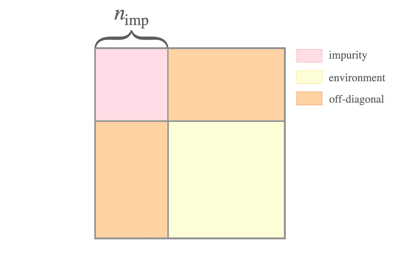
(a)

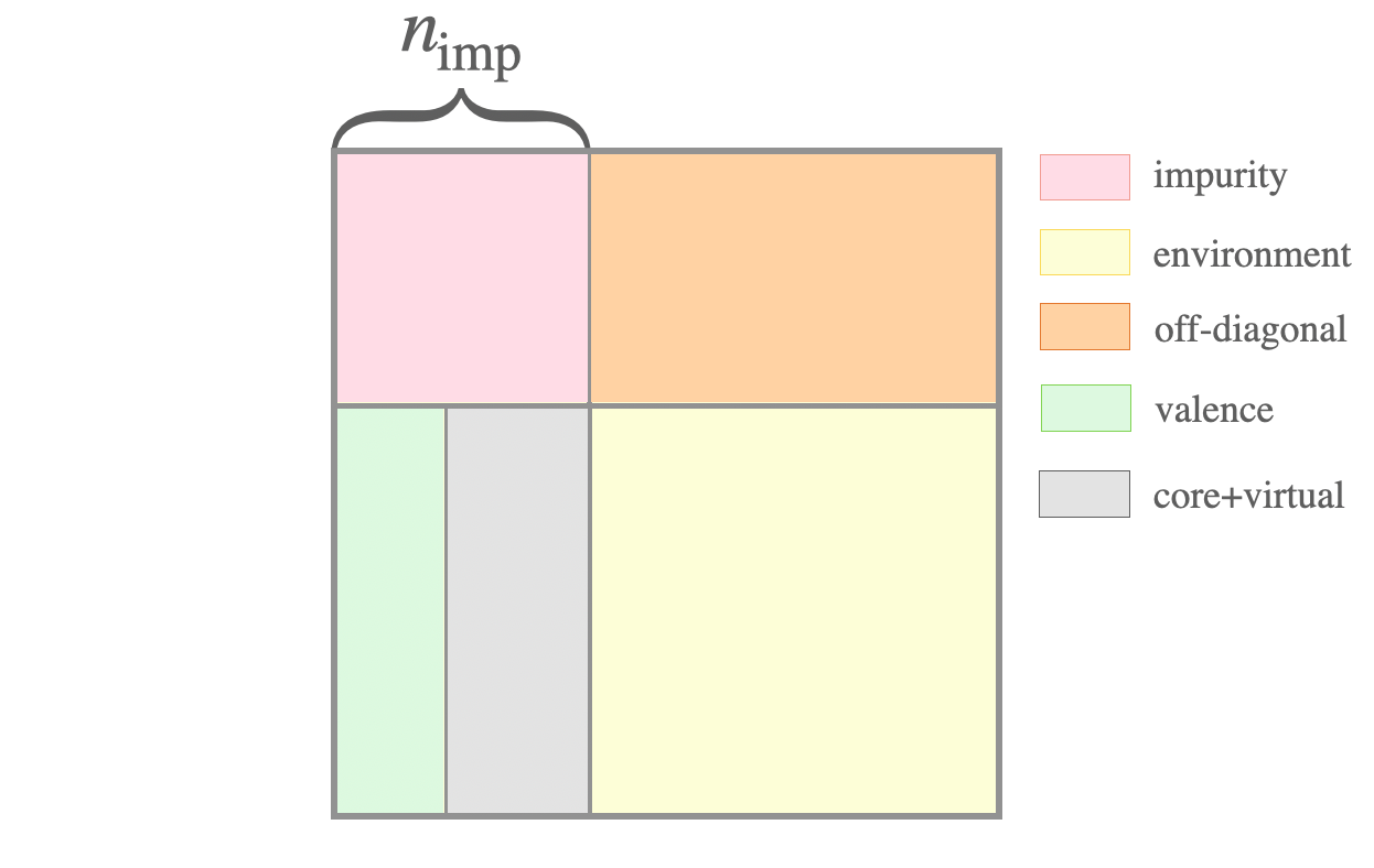
(b)

Figure 12: Bath orbitals from singular value decomposition (SVD) of the off-diagonal block of the mean-field density matrix. The whole square represents the mean-field density matrix of size $N\times N$, with $N$ being the total number of orbitals, and the first $n_{\text{imp}}$ columns/rows of the matrix are orbitals in the impurity. (a) Standard DMET routine computes the bath orbitals by the SVD of the off-diagonal block (orange blocks on the left and top, the block on the left corresponds to Eq. (49)). (b) Ab initio DMET computes the bath orbitals by the SVD of only the valence columns in the off-diagonal blocks (green block).

At finite temperature, electronic occupation numbers of the energy levels are ruled by the Fermi-Dirac distribution

$$f(\varepsilon_{i})=\frac{1}{1+e^{\beta(\varepsilon_{i}-\mu)}},$$ (52)

where $\varepsilon_{i}$ is the energy of the $i$th molecular orbital, $\beta=\frac{1}{T}$ is the inverse temperature (we set the Boltzmann’s constant $k_{B}=1$) and $\mu$ is the chemical potential or the energy of the Fermi level at ground state. When $\beta=\infty$, Eq. (52) reproduces the ground state electron number distribution: when $\varepsilon_{i}<\mu$, the occupation number is $1$ (occupied orbitals), and when $\varepsilon_{i}>\mu$, the occupation number is $0$ (virtual orbitals). However, when $\beta$ is finite, the electronic occupation number on virtual orbitals is no longer $0$. The extreme case is when $\beta=0$ where all energy levels are uniformly occupied with occupation number $f=0.5$. Therefore, the ground state bath construction described previously is no longer suitable to provide an accurate embedding Hamiltonian. There are generally two strategies: (1) include part of the core and virtual orbitals into the off-block for SVD; (2) obtain additional bath orbitals from higher powers of the mean-field density matrix [103]: take the valence columns of the off-diagonal blocks of $\gamma$, $\gamma^{2}$, …, $\gamma^{l}$ and apply SVD to them, respectively, to get $l$ sets of bath orbitals, then put the bath orbitals together and perform orthogonalization to produce the final bath orbitals. The disadvantage of the first strategy is obvious: as temperature gets higher, the Fermi-Dirac curve in Fig. 13 gets flatter, and thus more non-valence orbitals are needed. Compared to the first strategy, the latter strategy generally requires less number of bath orbitals. For most systems, truncating $l$ to $2$ or $3$ is already enough for the whole temperature spectrum, therefore the number of embedding orbitals is $n_{\text{imp}}+ln_{\text{val}}$. Since the number of valence orbitals is much smaller than that of the non-valence orbitals, DMET with bath orbitals derived from the second strategy is more economic and stable. In this paper, we adopt the second strategy for our FT-DMET calculations.

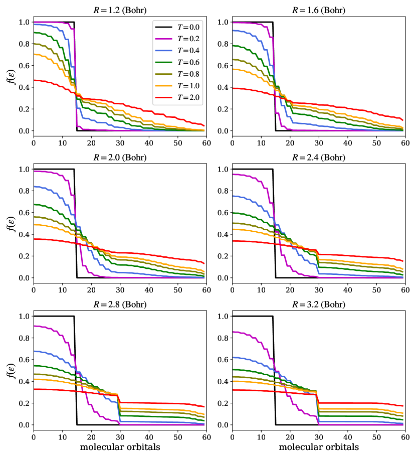
Figure 13: Fermi-Dirac distribution of electrons on Hartree-Fock molecular orbitals for H₃₀ chain with STO-6G basis. $T$ is in unit Hartree.

10.3 Embedding Hamiltonian

There are two choices of constructing the embedding Hamiltonian: (i) interacting bath formalism and (ii) non-interacting bath formalism  [42]. We pick the interacting bath formalism to restore most of the two-body interactions. The embedding Hamiltonian constructed from interacting bath formalism has the form

$$H_{\text{emb}}=\sum{pq}F^{\text{emb}}_{pq}c^{{\dagger}}_{p}c_{q}-\mu\sum_{p\in\text{imp}}c^{{\dagger}}_{p}c_{p}+\frac{1}{2}\sum_{pqrs}\left(pq|rs\right)c^{{\dagger}}_{p}c^{{\dagger}}_{r}c_{s}c_{q}.$$ (53)

Note that we use $p,q,r,s$ to index embedding orbitals and $i,j,k,l$ to index lattice orbitals. A chemical potential $\mu$ is added to only apply on the impurity, making sure that the number of electrons on the impurity is correct during the DMET self-consistency.

The embedding Fock matrix $F^{\text{emb}}$ is obtained by projecting the lattice Fock in AOs to the embedding orbitals. Using $\tilde{P}^{\mathbf{k}}=C^{\mathbf{k}}P^{\mathbf{k}}$ to denote the projection operator, one computes the embedding Fock matrix by

$$\tilde{F}=\frac{1}{N_{\mathbf{k}}}\sum_{\mathbf{k}}\tilde{P}^{\mathbf{k}\dagger}F^{\mathbf{k}}\tilde{P}^{\mathbf{k}}$$ (54)

where $F^{\mathbf{k}}$ is the lattice Fock matrix in $\mathbf{k}$-space AO basis. To avoid double counting, we subtract the contribution of the embedding electron repulsion integrals (ERIs) from $\tilde{F}$

$$F^{\text{emb}}_{pq}=\tilde{F}_{pq}-\left[\sum_{rs}\left(pq|rs\right)\gamma^{\text{emb}}_{sr}-\frac{1}{2}\left(pr|sq\right)\gamma^{\text{emb}}_{rs}\right]$$ (55)

where $\gamma^{\text{emb}}$ is the lattice density matrix rotated to the embedding space.

The time-consuming part is the construction and projection of the two-electron ERIs to the embedding space. To reduce the cost, we use density fitting [113, 114] to convert the four-center ERIs to the three-center ERIs,

$$\left(\mu\mathbf{k}_{\mu}\nu\mathbf{k}_{\nu}|\kappa\mathbf{k}_{\kappa}\lambda\mathbf{k}_{\lambda}\right)\approx\sum_{L\mathbf{k}_{L}}\left(\mu\mathbf{k}_{\mu}\nu\mathbf{k}_{\nu}|L\mathbf{k}_{L}\right)\left(L\mathbf{k}_{L}|\kappa\mathbf{k}_{\kappa}\lambda\mathbf{k}_{\lambda}\right)$$ (56)

where $L\mathbf{k}_{L}$ is the auxiliary basis and only three $\mathbf{k}$ indices are independent due to the conservation of momentum: $\mathbf{k}_{L}=\mathbf{k}_{\mu}-\mathbf{k}_{\nu}+n\mathbf{q}$ ($n\mathbf{q}$ is the integer multiple of reciprocal lattice vectors). The auxiliary basis used in this work is a set of chargeless Gaussian crystal orbitals with the divergent part of the Coulomb term treated in Fourier space [114]. Density fitting with the above auxiliary basis is called Gaussian density fitting (GDF). In practice, we first transform three-center ERIs from the lattice orbitals to the embedding orbitals with cost $\mathcal{O}\left(n_{\mathbf{k}}^{2}n_{L}n_{\text{lat}}n_{\text{emb}^{2}}+n_{\mathbf{k}}^{2}n_{L}n_{\text{lat}}^{2}n_{\text{emb}}\right)$; then we convert the three-center ERIs back to the four-center ERIs in the embedding space with cost $n_{\mathbf{k}}n_{L}n_{\text{emb}}^{2}$. The computational cost is significantly reduced compared to direct transformation with cost $\mathcal{O}\left(n_{\mathbf{k}^{3}n_{\text{lat}^{5}}}\right)$.

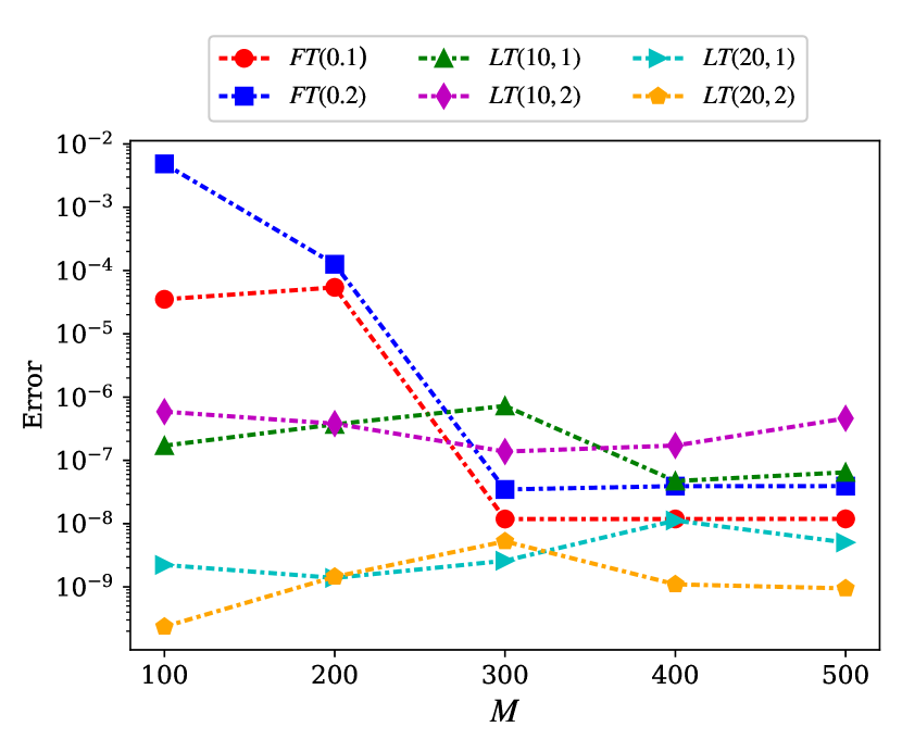
(a) $R=1.5$ Bohr

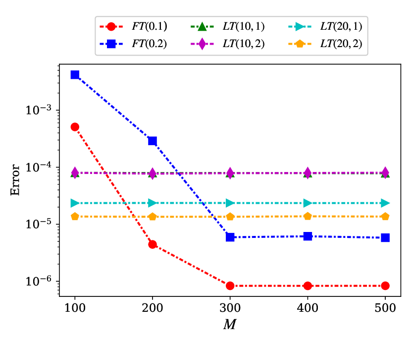
(b) $R=3.0$ Bohr

Figure 14: Accuracy test on FT-DMRG and LT-DMRG solvers against exact diagonalization. The label "FT($x$)" stands for FT-DMRG solver with $\tau=x$, and the label "LT($x,y$)" stands for LT-DMRG solver with $x$ Davidson roots and $y$ electron deviations from half-filling for both spins.

10.4 Impurity solver

An accurate finite temperature algorithm is required as the impurity solver. In this work, we use homemade finite temperature exact diagonalization (FT-ED) and finite temperature density matrix renormalization group (FT-DMRG) for small and large impurity problems, respectively. In particular, there are two ways to implement FT-DMRG: (1) imaginary time evolution from an enlarged Hilbert space, also known as the purification approach [29] (referred as FT-DMRG) ; and (2) using Davidson diagonalization to generate a set of low-energy levels to be used in the grand canonical statistics (referred as low temperature DMRG, LT-DMRG). While FT-DMRG can be used for the whole temperature spectrum, LT-DMRG is especially for low temperature calculations. Because most of the phase transitions happen at the low temperature regime, LT-DMRG can provide accurate enough calculations with lower cost compared to FT-DMRG.

Since FT-DMRG is based on imaginary time evolution from inverse temperature $\beta=0$, the entanglement grows rapidly as $\beta$ increases, and at low temperature a bond dimension that is much larger than the ground state bond dimension is required. Another error source of FT-DMRG is the imaginary time step $\tau=\beta/N$, where $N$ is the number of time steps. For symmetrized Trotter-Suzuki approximation, the local trucation error is on the order of $\mathcal{O}(\tau^{3})$, while the total accumulated error is on the order of $\mathcal{O}(\tau^{2})$. If the 4th order Runge-Kutta (RK4) method is used, the local truncation error is on the order of $\mathcal{O}(\tau^{5})$ and the total accumulated error is on the order of $\mathcal{O}(\tau^{4})$. The FT-DMRG used in the calculations of this work used the RK4 method. Note that since the matrix product state (MPS) truncation is applied at every time step, having a too small $\tau$ will lead to a large accumulation of MPS truncation errors. Therefore, one needs to choose the $\tau$ value to be not too small to introduce large MPS truncation errors and not too big to introduce large time evolution truncation errors. The error source of LT-DMRG is from the truncation of the grand canonical summation and the number of roots in the Davidson diagonalization. Generally the ground state bond dimension is enough for the low temperature calculations with LT-DMRG.

An assessment of the accuracy of FT-DMRG and LT-DMRG solvers is shown in Fig. 14. The embedding system is composed of two impurity orbitals and two bath orbitals, generated from a $6$-site hydrogen chain with the STO-6G basis at $R=1.5$ and $3.0$ Bohr at $\beta=20$. Exact diagonalization (ED) is chosen as the exact reference. In Fig. 14, we try to understand the role of imaginary time step $\tau$ in FT-DMRG solver and the roles of the number of Davidson roots and the size of the truncated grand canonical space in the LT-DMRG solver. At $\beta=20$, the smaller $\tau$ (red lines) gave a smaller error compared to $\tau=0.2$ (blue lines), and the FT-DMRG results converged at $M\sim 300$. The errors of LT-DMRG solver do not change too much with the bond dimension $M$, so $M=100$ is already enough for a $4$-site system. The accuracy at $R=1.5$ Bohr is generally better than $R=3.0$ Bohr, since larger $R$ corresponds to stronger correlation. At larger $R$, one needs to include a larger number of Davidson roots to achieve high enough accuracy with LT-DMRG. Generally with large enough bond dimension $M$, FT-DMRG could provide more accurate results. However, when the embedding system is too large to use a large $M$, one could consider the LT-DMRG method. In DMET calculations, we use $ED$ solver for $L_{\text{emb}}<8$ embedding problems and use FT-DMRG solver for larger problems.

10.5 Thermal observables

In order to identify the metal-insulator transition and the Néel transition and explore the mechanism behind the crossings, we compute the following order parameters: staggered magnetic moment $m$, double occupancy $D$, complex polarization $Z$, spin-spin correlation functions $\mathcal{C}_{ss}$, and charge-charge correlation functions $\mathcal{C}_{cc}$.

Staggered magnetic moment. The staggered magnetic momentum is calculated as

$$m=\frac{1}{N^{\text{imp}}}\sum_{i\in\text{imp}}\frac{|n_{i,\uparrow}-n_{i,\downarrow}|}{2},$$ (57)

where $N^{\text{imp}}$ is the total number of H atoms in the impurity (supercell), and $n_{i,\uparrow}$ and $n_{i,\downarrow}$ are electron numbers on $i$th atom with up spin and down spin, respectively. Note that if one uses Bohr magneton $\mu_{B}=\frac{e\hbar}{2m_{e}}=\frac{1}{2}$ as the unit, then one would drop $2$ in the denominator in Eq. (57). To evaluate $n_{i,\uparrow}$ on the $i$th atom, we first compute the one-particle impurity density matrix for up-spin in the IAO basis, and then sum up the diagonal terms that belong to the $i$th atom. For example, when STO-6G basis is used, the occupation numbers on $1s$ orbital and $2s$ orbital of atom-$i$ sum up to the electron density on atom-$i$. $n_{i,\downarrow}$ is evaluated in the same way from the down-spin one-particle impurity density matrix.

Double occupancy. The double occupancy measures the probability of two electrons with opposite spins occupying the same hydrogen atom, calculated by

$$D=\frac{1}{N^{\text{imp}}}\sum_{i\in\text{imp}}\langle\hat{n}_{i\uparrow}\hat{n}_{i,\downarrow}\rangle.$$ (58)

Note that the hat on $\hat{n}_{i\uparrow}$ denotes that it is an operator, not a number, with $n_{i\uparrow}=\langle\hat{n}_{i\uparrow}\rangle$. Since there are multiple bands on each atom, we expand $\hat{n}_{i\uparrow}$ as

$$\hat{n}_{i\uparrow}=\sum_{w}\hat{n}^{w}_{i\uparrow},$$ (59)

where $w$ is the index of the bands on the $i$-th atom ( e.g., $1s$, $2s$, $2p_{x},2p_{y},2p_{z},...$). Therefore, the precise expression of double occupancy becomes

$$D=\frac{1}{N^{\text{imp}}}\sum_{i\in\text{imp}}\sum_{w,w^{\prime}\in i}\langle\hat{n}^{w}_{i\uparrow}\hat{n}^{w^{\prime}}_{i,\downarrow}\rangle.$$ (60)

Complex polarization. Complex polarization measures the mobility of electrons, and thus can be used as an indicator of metal-insulator transition. The definition of complex polarization on $z$ direction is

$$Z=\langle e^{i\frac{2\pi}{L}\hat{z}}\rangle,$$ (61)

where $L$ is the chain length and $\hat{z}$ is the location operator in the $z$-direction. When $Z=0$, electrons are delocalized and the system is metallic; when $Z=1$, electrons are localized and the system is insulating. At mean-field level, the ground state is a Slater determinant $|\phi\rangle$ of occupied orbitals, so the complex polarization is evaluated by

$$Z=\langle\phi|e^{i\frac{2\pi}{L}\hat{z}}|\phi\rangle,$$ (62)

which is equivalent to

$$Z=\text{Det}\left[C_{\text{occ}}^{{\dagger}}e^{i\frac{2\pi}{L}z}C_{\text{occ}}\right],$$ (63)

where $C_{\text{occ}}$ represents the coefficients of occupied orbitals.

At finite temperature, we use a thermofield approach [115] from our recent work (see Chapter 4). We construct the infinite temperature determinant with an enlarged Hilbert space $\tilde{\phi}$, and thermofield operators of the Hamiltonian $\tilde{H}$ and position operator $\tilde{z}$. Then the finite temperature complex polarization is evaluated by

$$Z(\beta)=\frac{1}{\mathcal{Z}}\langle\tilde{\phi}|e^{-\beta(\tilde{H})}e^{i\frac{2\pi}{L}\tilde{z}}|\tilde{\phi}\rangle,$$ (64)

where $\mathcal{Z}\langle\tilde{\phi}|e^{-\beta(\tilde{H})}|\tilde{\phi}\rangle$ is the partition function.

Spin-spin correlation and charge-charge correlation functions. We define the two correlation functions as follows:

$$\begin{split}\mathcal{C}^{ss}_{i}=&\langle(\hat{n}_{0}^{\uparrow}-\hat{n}_{0}^{\downarrow})(\hat{n}_{i}^{\uparrow}-\hat{n}_{i}^{\downarrow})\rangle-\langle\hat{n}_{0}^{\uparrow}-\hat{n}_{0}^{\downarrow}\rangle\langle\hat{n}_{i}^{\uparrow}-\hat{n}_{i}^{\downarrow}\rangle,\\ \mathcal{C}^{cc}_{i}=&\langle(\hat{n}_{0}^{\uparrow}+\hat{n}_{0}^{\downarrow})(n_{i}^{\uparrow}+n_{i}^{\downarrow})\rangle-\langle\hat{n}_{0}^{\uparrow}+\hat{n}_{0}^{\downarrow}\rangle\langle n_{i}^{\uparrow}+n_{i}^{\downarrow}\rangle,\end{split}$$ (65)

where $\hat{n}_{i}^{\sigma}$ is the electron density operator of spin $\sigma$ on site $i$.

11 Results

In this section, we show some preliminary results of FT-DMET calculations on the hydrogen chain system with periodic boundary condition. First, we examine the basis set effect on a $22$-atom chain with $2$ atoms in the impurity. Fig. 15 shows the magnetic moment at both ground state and $T=0.02$ Hartree calculated by DMET with STO-6G, 6-31G, and CC-PVDZ basis sets. Paramagnetic-antiferromagnetic (PM-AFM) transition is observed at both ground state and $T=0.02$ Hartree. A very interesting behavior of the magnetic moment at ground state is observed: with STO-6G, the magnetic moment drops at $R>3.0$ Bohr, while with larger basis sets, this drop did not happen. The reason for the above behaviors could be due to the loss of entanglement between different sites at large $R$. Imagine at $R=\infty$, the system should behave as $22$ individual atoms, and one should expect the ground state to be paramagnetic. With more diffused orbitals (e.g., $2s$ and $2p$ orbitals), however, the entanglement between different sites decays slower as $R$ increases. Note that since the impurity size is only $2$ atoms, one only needs to consider the entanglement between adjacent sites. Once the impurity gets larger, a drop of magnetic moment with larger basis sets should also be expected. At $T=0.02$ (left panel), the magnetic moment computed with all three basis sets dropped as $R$ increases, as a consequence of thermal dissipation.

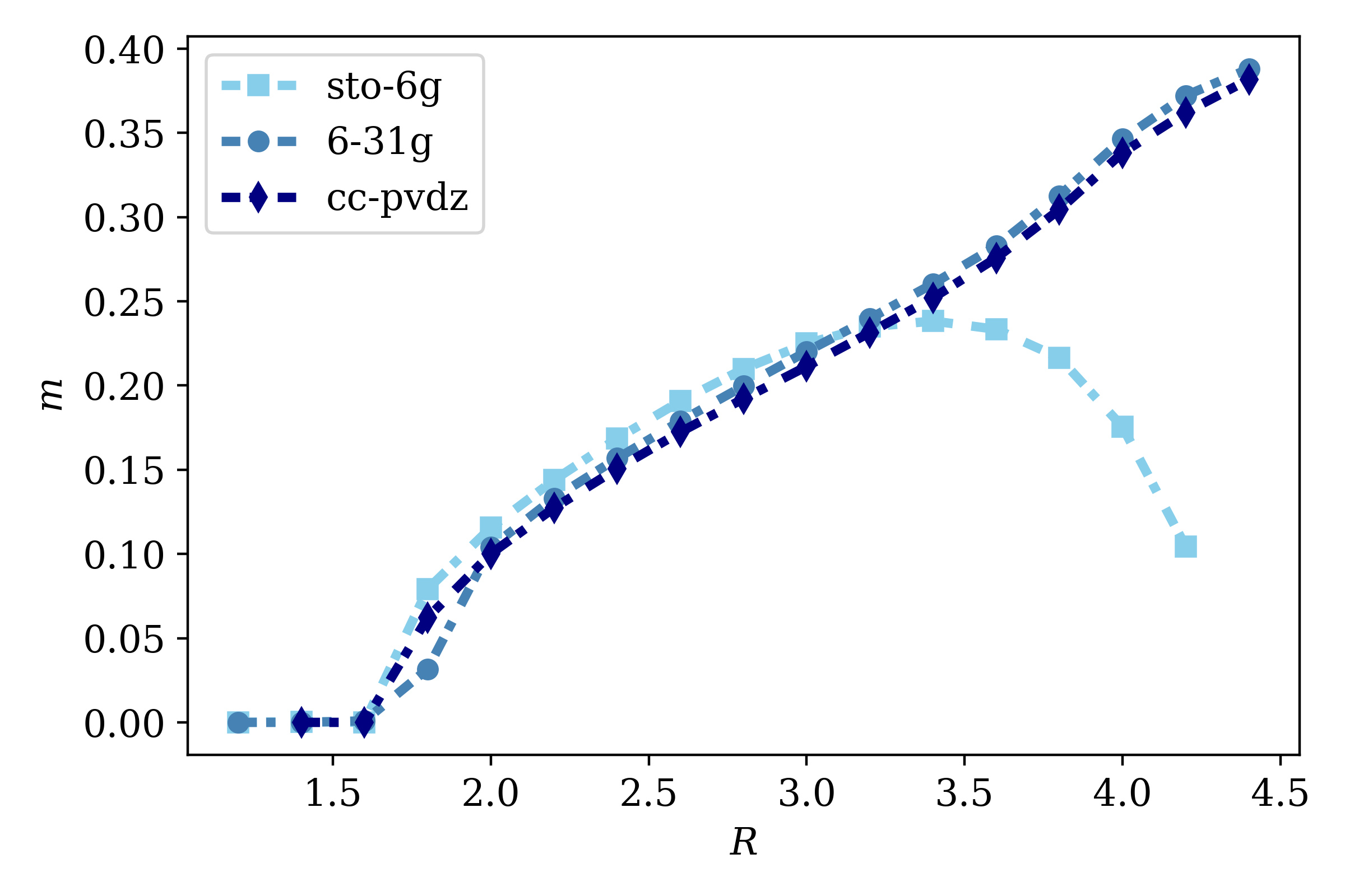
(a)

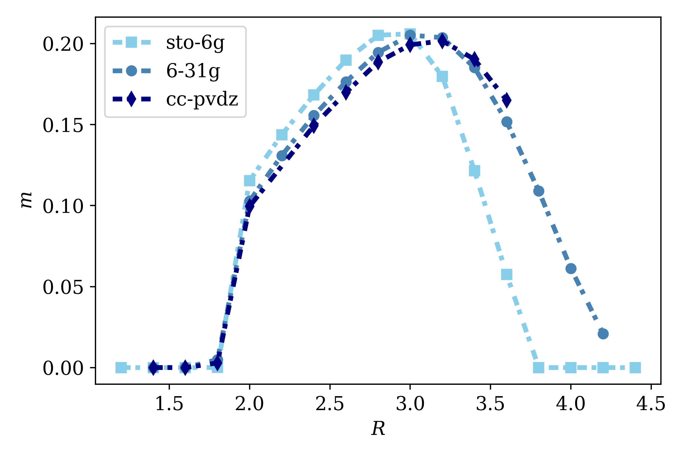
(b)

Figure 15: Magnetic moment of a $22$-atom chain at ground state (left panel) and $T=0.02$ Hartree (right panel) with STO-6G, 6-31G, and CC-PVDZ basis sets.

We further show the double occupancy from the above simulation settings in Fig. 16. A clear change of the gradient of $D$ as a function of $R$ is observed for both ground state and $T=0.02$ Hartree, indicating a metal to insulator transition. The transition $R$ is around $1.6\sim 1.8$ Bohr, which agrees with the transition $R$ of PM-AFM transition, resulting in a PM metal phase and AFM insulating phase.

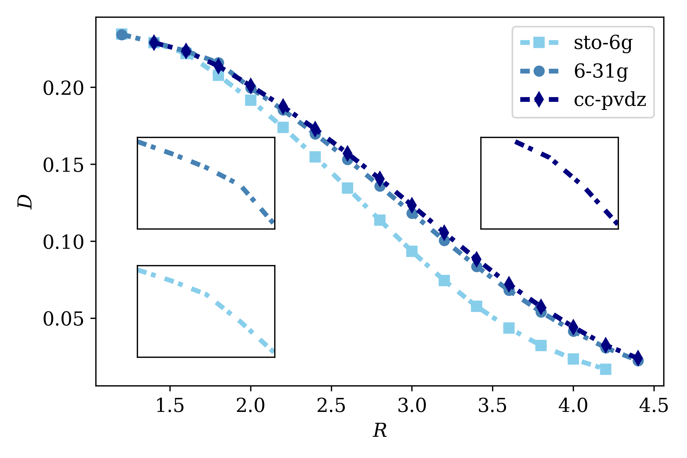
(a)

(b)

Figure 16: Double occupancy of a $22$-atom chain at ground state (left panel) and $T=0.02$ Hartree (right panel) with STO-6G, 6-31G, and CC-PVDZ basis sets. The insets show a sudden change of the gradient of $D$ as a function of $R$, indicating metal to insulator transition.

Next we increase the total number of atoms in the hydrogen chain to $50$ atoms to eliminate the finite size effect of the total system size. STO-6G is used as the basis set. The impurity is composed of two hydrogen atoms, and solved by ED. We first present the energy calculations and dissociation curve of the hydrogen chain, shown in Fig. 17, where the energy per electron at $T=0.05$ is compared to FT-AFQMC [5] results. The AFQMC calculation used the STO-6G basis set and a supercell with $10$ atoms and $5$ $k$ points. The two energy curves predicted the same dissociating trend and equilibrium point ($\sim 1.8$ Bohr). However, the DMET energies are all lower than the AFQMC energies, which could be due to the finite impurity size effect.

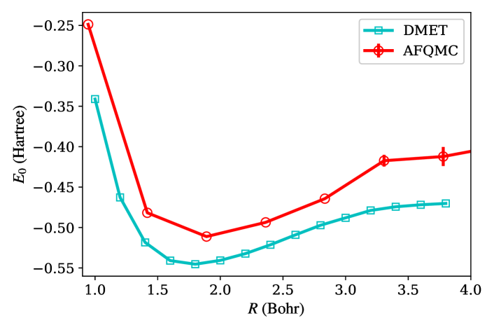
Figure 17: Dissociation curve of hydrogen chain at $T=0.05$ Hartree compared to AFQMC. The AFQMC data is extracted from Ref. [5].

We then examine the staggered magnetic moment $m$ as a function of inter-atomic distance $R$ at ground state, $T=0.02$, $T=0.05$, and $T=0.1$ in Fig. 18. Compared to Fig. 15 where the paramagnetic-antiferromagnetic (PM-AFM) transition happened around $R=1.6$ Bohr, we observed the PM-AFM transition at $R=1.0\sim 1.5$ region for $T<0.1$, which could be an effect of the finite total system size. Although $T=0.02$ is considered as very close to the ground state, the magnetic moment at $T=0.02$ drops earlier than the ground state curve as $R$ increases. This behavior is due to the thermal dissipation of the magnetic order. As $R$ grows larger, the atoms are far apart from each other, and thus the electron-electron correlation between different sites is weaker, and eventually not enough to preserve the long-range AFM order, which lead to the drop of magnetic order at large $R$ as shown in the figure. Even adding a small temperature, the flip of the spin can happen to destroy the long-range AFM order.

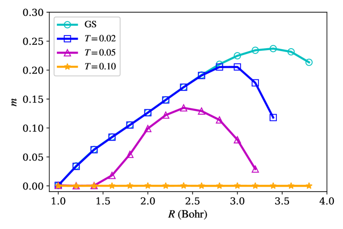
Figure 18: Staggered magnetic moment of hydrogen chain with periodic boundary condition at ground state, $T=0.02$, $T=0.05$, and $T=0.1$. The unit of $T$ is Hartree.

12 Conclusion

In this work, we generalized the previously described finite temperature density matrix embedding theory to study ab initio solid, and employed the method to study the hydrogen chain problem. Despite the simplicity of the hydrogen chain lattice compared to other periodic systems, it exhibits a variety of intriguing behaviors including paramagnetic-antiferromagnetic transition and metal-insulator transition at both ground state and finite temperature. At finite temperature, we observed thermal dissipation for the magnetic order at large inter-atomic distance. We further confirmed the stabilizing effect from multi-band basis sets. Since this work is not completely finished, in the future we will apply this finite temperature algorithm to a larger set of ab initio solids including the two-dimensional and three-dimensional hydrogen lattices, transition metal oxides, and challenging systems such as cuprate-based high temperature superconductors.

Chapter 4 Finite temperature complex polarization and metal-insulator transition

13 Abstract

Metal-insulator transition is a fundamental yet complicated topic in condensed matter physics and material science. Band structure theory has been widely used in explaining why insulators are insulating and why metals are conducting, but can fail to describe insulation phases caused by strong correlations or disorder. Electron locality/mobility serves as a more general indicator of metallic and insulating phases: when the system is metallic, the electrons are delocalized and can flow freely; when the system is insulating, the electrons are localized. The standard deviation (or second cumulant moment) of the electron position is used as the order parameter of the electron localization, which is directly related to the complex polarization of the system. The complex polarization is widely accepted as a new indicator of the metal-insulator transition at ground state: when the complex polarization equals zero, the second cumulant moment of the position is diverged and the system sits in the metallic phase; when the complex polarization is nonzero, the electrons are localized and the insulating phase wins. In this work, we present the finite temperature formulation of the complex polarization. We also introduce a thermofield approach to compute the complex polarization with thermal Slater determinant. We demonstrate how finite temperature complex polarization works as an indicator of metal-insulator transition at low temperature with a modified tight binding model and hydrogen chain system. In the hydrogen chain case, we also compare the metal-insulator transition with the paramagnetic-ferromagnetic transition, electron population, and energy gap to study the origin of the insulating and metallic phases, respectively.

14 Introduction

Phase transition happens when a system undergoes a macroscopic change from one phase to another phase due to the variation of control parameters such as temperature, magnetic field, chemical substitution, and pressure. Near the critical point between the two phases, the physical properties of the bulk changes dramatically with respect to even a minor perturbation in control parameters. Metal-insulator transition (MIT) is among the most common phase transitions, yet the microscopic cause and the physics behind the phenomena is nontrivial. From the elementary physics textbooks, we learned that metals are conducting when an electrical field is applied, while insulators do not allow electrons to flow freely. However, this is a rather vague and bipartite definition, which is not able to answer questions such as (1) what are the microscopic driving forces for conductivity? (2) what are the causes for MIT? and (3) how does one characterize MIT?

In the past, the microscopic featurization of insulators and metals are generally described by the band structure theory [116, 117]. The band structure theory describes the movement of a single electron in a periodic solid, with the mean-field effect from the other electrons. According to band structure theory, if the Fermi level sits in a band gap, then the system is insulating; if the Fermi level crosses a band, the system is conducting. However, the band structure theory is based on independent electron approximation and is only limited to crystalline systems. The insulating behavior caused by disorder or electron-electron correlation cannot be captured accurately by the band structure theory [118, 119, 120, 121]. A more general description is to use the electron localization to distinguish metal and insulator: when the electrons are localized, the system is insulating, and when the electrons are delocalized, the system is conducting. A widely accepted approach to evaluate electron localization is based on the theory of polarization [122, 123, 124, 125, 126, 127, 128, 129], where the macroscopic polarization is connected to Berry phase [130]. A more straightforward indicator of electron localization is the second cumulant moment of the electron position operator describing the spread of electrons [129, 131, 123, 124, 125]. A value that connects to both the macroscopic polarization and the second cumulant moment is complex polarization: the phase of the complex polarization is the Berry phase, while the second cumulant moment can be evaluated from the modulo of the complex polarization [132, 133, 134]. Moreover, the DC conductivity according to the ground state Kubo formula [135] is also related to the modulo of the complex polarization.

Ground state complex polarization and its connection to macroscopic polarization, electron localization, and DC conductivity have been thoroughly studied and discussed in the past [129, 131, 133]. However, discussion about finite temperature complex polarization is rare, regardless of the significance of this parameter. In this work, we introduce the formulation of finite temperature complex polarization and discuss its relationship with electron localization. We also present a mean-field level implementation of finite temperature complex polarization under thermofield theory  [136, 137, 138, 115]. In Section 15, we introduce the ground state formulation of complex polarization and electron localization, where we first use the single particle case as a simplified example and then generalize the single particle case to many-body mean-field formulation. In Section 16, we extend the ground state formulation to the finite temperature version, and present a thermofield approach to evaluate the complex polarization. In Section 17, we apply the finite temperature formulation to a modified tight binding model both analytically and numerically, presenting a preliminary analysis of how complex polarization provides information of metal-insulator transition. In Section 18, we choose hydrogen chain as an example of computing finite temperature complex polarization for ab initio systems and explore the temperature-induced metal-insulator transition in the hydrogen chain. We finalize this article with a summary and outlook in Section 19.

15 Ground state complex polarization and electron localization

The many-body complex polarization $Z_{N}^{(\alpha)}$ was first introduced as the ground state expectation value of certain unitary many-body operators  [128]. We start by defining a general form of the unitary many-body operator

$$\hat{U}(\mathbf{k})=e^{i\mathbf{k}\cdot\hat{\mathbf{R}}},$$ (66)

where $\mathbf{k}$ is an arbitrary three-dimension vector and $\hat{\mathbf{R}}$ is the three-dimensional position operator, with $\hat{R}^{\alpha}\psi(r_{1},r_{2},r_{3})=r_{\alpha}\psi(r_{1},r_{2},r_{3}),\alpha=1,2,3$.

We introduce three $\mathbf{k}$ vectors with notation $\mathbf{\kappa}^{(\alpha)}(\alpha=1,2,3)$, defined as

$$\kappa^{(\alpha)}_{\beta}=\frac{2\pi}{L}\delta_{\alpha\beta},$$ (67)

which can be explicitly written as

$$\begin{split}\kappa^{(1)}&=\left(\frac{2\pi}{L},0,0\right),\\ \kappa^{(2)}&=\left(0,\frac{2\pi}{L},0\right),\\ \kappa^{(3)}&=\left(0,0,\frac{2\pi}{L}\right).\end{split}$$ (68)

The ground state complex polarization is then defined as the expectation values of the unitary many-body operators with the above three vectors:

$$Z_{N}^{(\alpha)}=\langle\Psi_{0}|\hat{U}(\mathbf{\kappa}^{\alpha})|\Psi_{0}\rangle,$$ (69)

where $N$ is the number of electrons and $|\Psi_{0}\rangle$ represents the ground state of the system of interest. The complex polarization $Z_{N}^{(\alpha)}$ in Eq. (69) can be explicitly written as

$$Z_{N}^{(\alpha)}=|Z_{N}^{(\alpha)}|e^{i\gamma^{(\alpha)}_{N}},$$ (70)

where $|Z_{N}^{(\alpha)}|\in[0,1]$ is the modulo of $Z_{N}^{(\alpha)}$ and $\gamma^{(\alpha)}_{N}$ is the phase of $Z_{N}^{(\alpha)}$, referred as the Berry phase. In this article, we will not discuss the macroscopic polarization, therefore the phase of Eq. (70) will not be mentioned. In fact, with a centrosymmetric choice of the origin, the complex polarization will always remain real.

15.1 Electron localization

We start by considering a problem with one particle in a one-dimensional potential wall. The locality of the particle can be measured by the quadratic spread, or the second cumulant moment of the position $x$, defined as

$$\langle\delta x^{2}\rangle=\langle\psi|x^{2}|\psi\rangle-\langle\psi|x|\psi\rangle^{2},$$ (71)

where $|\psi\rangle$ is the ground state of the particle in a box. $\langle\delta x^{2}\rangle$ is finite when the state $|\psi\rangle$ is bounded and diverges for an unbounded state. Let $n(x)=|\psi(x)|^{2}$ be the electron density, then we can rewrite Eq. (71) as

$$\langle\delta x^{2}\rangle=\int_{-\infty}^{\infty}\mathrm{d}x\ x^{2}n(x)-\left(\int_{-\infty}^{\infty}\mathrm{d}x\ xn(x)\right)^{2}.$$ (72)

We now assume that $\psi(x)$ is periodic with wavelength $L$

$$\psi(x+mL)=\psi(x),$$ (73)

where $m$ is an integer. The Fourier transformation of $n(x)$ gives

$$\tilde{n}(k)=\int_{-\infty}^{\infty}e^{-ikx}n(x).$$ (74)

We chose the origin to be $x_{0}$ so that $\langle x\rangle=0$, then

$$\int_{-\infty}^{\infty}\mathrm{d}x\ xn(x)=-i\frac{\mathrm{d}\tilde{n}(k)}{\mathrm{d}k}\Biggr{|}_{k=0}=0,$$ (75)

and $\langle\delta x^{2}\rangle$ is only evaluated from the average value of $x^{2}$

$$\langle\delta x^{2}\rangle=\int_{-\infty}^{\infty}\mathrm{d}x\ x^{2}n(x)=-\frac{\mathrm{d}^{2}\tilde{n}(k)}{\mathrm{d}k^{2}}\Biggr{|}_{k=0}.$$ (76)

Combining Eq. (75) and Eq. (76), we can approximate $\tilde{n}(k)$ with the Taylor expansion up to the second order

$$\tilde{n}(k)\approx 1-\frac{1}{2}\langle\delta x^{2}\rangle k^{2}.$$ (77)

Now we can write down the single particle complex polarization modified from Eq. (69) as

$$z=e^{i\frac{2\pi}{L}x_{0}}\tilde{n}\left(-\frac{2\pi}{L}\right).$$ (78)

Combining Eq. (77) and Eq. (78), we get the relationship between the complex polarization $z$ and second accumulant moment $\langle\delta x^{2}\rangle$

$$\langle\delta x^{2}\rangle\approx 2\left(\frac{2\pi}{L}\right)^{2}.(1-|z|)$$ (79)

One could also rewrite Eq. (77) as the exponential form

$$\tilde{n}(k)\approx e^{-\frac{1}{2}\langle\delta x^{2}\rangle k^{2}},$$ (80)

where we took $-\frac{1}{2}\langle\delta x^{2}\rangle k^{2}$ in Eq. (77) as the first order of the Taylor expansion of an exponential instead of the second order. From Eq. (80), one gets

$$\langle\delta x^{2}\rangle\approx-2\left(\frac{L}{2\pi}\right)^{2}\log|z|.$$ (81)

For a localized state, both Eq. (79) and Eq. (81) go to the same finite limit for large $L$; for a delocalized state, Eq. (81) is preferred since it diverges at $|z|=0$.

Eq. (81) gives us a straightforward relationship between the complex polarization $z$ and second cumulant moment $\langle\delta x^{2}\rangle$: when the system is insulating with $0<|z|\leq 1$, $\langle\delta x^{2}\rangle$ is finite and the ground state is localized; when the system is metallic with $|z|=0$, $\langle\delta x^{2}\rangle$ diverges and the ground state is delocalized. Therefore, one could use $z$ as a direct indicator of the locality of the electrons.

Similarly, the many-body electron localization is defined as

$$\langle\delta x^{2}\rangle\approx-\frac{2}{N}\left(\frac{L}{2\pi}\right)^{2}\log(|Z_{N}|),$$ (82)

where $Z_{N}$ is the many-body complex polarization.

15.2 Complex polarization for independent electrons

When there is no interaction among electrons, the ground state can be expressed as a Slater determinant $|\Psi_{0}\rangle$, and the complex polarization can be written as

$$Z_{N}^{(\alpha)}=\langle\Psi_{0}|\hat{U}(\mathbf{\kappa}^{(\alpha)})|\Psi_{0}\rangle=\langle\Psi_{0}|\Phi_{0}\rangle,$$ (83)

where $\hat{U}(\mathbf{\kappa}^{(\alpha)})=e^{i\mathbf{\kappa}^{(\alpha)}\cdot\mathbf{r}}$ and $|\Phi_{0}\rangle=\hat{U}(\mathbf{\kappa}^{(\alpha)})|\Psi_{0}\rangle$.

According to the Thouless theorem [139, 140], $|\Phi_{0}\rangle$ is also a determinant composed of orbitals rotated from the orbitals in $\Psi_{0}$ as

$$\phi_{\mu}(\mathbf{r})=e^{i\mathbf{\kappa}^{(\alpha)}\cdot\mathbf{r}}\psi_{\mu}(\mathbf{r}).$$ (84)

Therefore, $Z_{N}^{(\alpha)}$ is equal to the overlap between $|\Psi_{0}\rangle$ and $\Phi_{0}\rangle$. The overlap of two Slater determinants are evaluated by the determinant of the $N\times N$ overlap matrix $\mathcal{S}^{(\alpha)}$ evaluated by

$$\mathcal{S}_{\mu\nu}^{(\alpha)}=\int\mathrm{d}\mathbf{r}\psi_{\mu}^{*}(\mathbf{r})e^{i\mathbf{\kappa}^{(\alpha)}\cdot\mathbf{r}}\psi_{\nu}(\mathbf{r}),$$ (85)

where $\psi_{\mu}(\mathbf{r})$ are occupied orbitals.

The many-body complex polarization is then evaluated as

$$Z_{N}^{(\alpha)}=\left(\text{det}\mathcal{S}^{(\alpha)}_{\uparrow}\right)\left(\text{det}\mathcal{S}^{(\alpha)}_{\downarrow}\right),$$ (86)

where the indices $\uparrow$ and $\downarrow$ correspond to up and down spins. Eq. (86) can be applied to numerical calculations where Slater determinants can be obtained to represent the state of the system. The above numerical algorithms include the Hartree-Fock method, the density functional theory (DFT), Slater determinant based quantum Monte Carlo (QMC) methods, etc.

16 Finite temperature complex polarization

At finite temperature, the expectation value (thermal average) of an operator $\hat{A}$ is evaluated under the grand canonical ensemble

$$\begin{split}\langle\hat{A}\rangle(\beta)&=\frac{1}{\mathcal{Q}}\text{Tr}\langle\hat{A}\hat{\rho}\rangle\\ &=\frac{1}{\mathcal{Q}}\sum_{n}\langle n|\hat{A}e^{-\beta\hat{H}}|n\rangle,\end{split}$$ (87)

where $\beta$ is the inverse temperature, $\hat{H}$ is the Hamiltonian with the chemical potential, $\{|n\rangle\}$ forms a set of orthonormal basis, $\hat{\rho}=e^{-\beta\hat{H}}$ is the density matrix, and $\mathcal{Q}$ is the partition function defined as

$$\mathcal{Q}=\sum_{n}\langle n|e^{-\beta\hat{H}}|n\rangle.$$ (88)

According to the thermofield theory, the ensemble average in Eq. (87) can be expressed as an expectation value over one state $|\Psi(\beta)\rangle$, known as the thermofield double state or simply thermal state

$$\langle\hat{A}\rangle(\beta)=\frac{\langle\Psi(\beta)|\hat{A}|\Psi(\beta)\rangle}{\langle\Psi(\beta)|\Psi(\beta)\rangle}.$$ (89)

In thermofield theory, a copy of the original Hilbert space $\mathcal{H}$ is introduced as $\tilde{\mathcal{H}}$, known as the auxiliary space. At infinite temperature ($\beta=0$), the thermal state is given by a uniform summation over the orthonormal basis

$$|\Psi(0)\rangle=\sum_{n}|n\rangle\otimes|\tilde{n}\rangle,$$ (90)

where $\{|\tilde{n}\rangle\}$ are copies of $\{|n\rangle\}$ in the auxiliary space.

The thermal state at $\beta$ is then derived by imaginary time evolution from $|\Psi(0)\rangle$

$$|\Psi(\beta)\rangle=e^{-\beta\hat{H}/2}|\Psi(0)\rangle.$$ (91)

Note that the Hamiltonian $\hat{H}$ only acts on the original Hilbert space $\mathcal{H}$. Eq. (89) can be rewritten as

$$\begin{split}\langle\hat{A}\rangle(\beta)&=\frac{\langle\Psi(0)|e^{-\beta\hat{H}/2}\hat{A}e^{-\beta\hat{H}/2}|\Psi(0)\rangle}{\langle\Psi(0)|e^{-\beta\hat{H}}|\Psi(0)\rangle}\\ &=\frac{\langle\Psi(0)|e^{-\beta\hat{H}}\hat{A}|\Psi(0)\rangle}{\langle\Psi(0)|e^{-\beta\hat{H}}|\Psi(0)\rangle}.\end{split}$$ (92)

The complex polarization at temperature $T=1/\beta$ is thus

$$Z_{N}(\beta)=\frac{\langle\Psi(0)|e^{-\beta\hat{H}}\hat{Z}|\Psi(0)\rangle}{\langle\Psi(0)|e^{-\beta\hat{H}}|\Psi(0)\rangle},$$ (93)

where $\hat{Z}=e^{-i\frac{2\pi}{L}\hat{x}}$. Note that for simplicity, we dropped the superscript $(\alpha)$ and chose only the $x$ component of the three-dimensional position operator $\hat{\mathbf{r}}$. This simplification is valid for a one-dimensional system, and for multi-dimensional systems, $Z_{N}$ of other directions can be evaluated in the same manner.

At the mean-field level, thermal state $|\Psi_{0}\rangle$ can be written as a Slater determinant formed by the following $2L\times L$ coefficients

$$C_{0}=\begin{bmatrix}1&0&0&\cdots&0\\ 0&1&0&\cdots&0\\ 0&0&1&\cdots&0\\ 0&0&0&\ddots&0\\ 0&0&0&\cdots&1\\ 1&0&0&\cdots&0\\ 0&1&0&\cdots&0\\ 0&0&1&\cdots&0\\ 0&0&0&\ddots&0\\ 0&0&0&\cdots&1\\ \end{bmatrix}=\begin{bmatrix}\mathbb{I}\\ \mathbb{I}\end{bmatrix},$$ (94)

where the first $L$ rows correspond to the physical sites, and the last $L$ rows correspond to the auxiliary sites. A one-body operator $\hat{w}$ in $\mathcal{H}$ is rewritten as

$$\bar{\hat{w}}=\hat{w}\oplus 0.$$ (95)

Under Hartree-Fock approximation, we use the Fock operator $\hat{f}$ as the one-body Hamiltonian, and the matrix form of the thermal Fock operator $\bar{\hat{f}}$ is

$$\left[\bar{\hat{f}}\right]=\begin{bmatrix}[\hat{f}]&0\\ 0&0\end{bmatrix}.$$ (96)

The position operator $\hat{x}$ is also a one-body operator, with the matrix form as

$$\left[\bar{\hat{x}}\right]=\begin{bmatrix}[\hat{x}]&0\\ 0&0\end{bmatrix}.$$ (97)

The thermal density operator $\bar{\hat{\rho}}=e^{-\beta\bar{\hat{f}}}$, with the matrix form

$$\left[\bar{\hat{\rho}}\right]=\begin{bmatrix}\left[e^{-\beta\hat{f}}\right]&0\\ 0&\mathbb{I}\\ \end{bmatrix}.$$ (98)

The thermofield expression of the complex polarization operator $e^{i\frac{2\pi}{L}\hat{x}}$ therefore has the matrix form

$$\left[\bar{\hat{Z}}\right]=\begin{bmatrix}\left[e^{i\frac{2\pi}{L}\hat{x}}\right]&0\\ 0&\mathbb{I}\end{bmatrix}.$$ (99)

The complex polarization at $\beta$ can be evaluated by a similar formulation as ground state

$$Z_{N}(\beta)=\frac{\text{det}\left(C_{0}^{{\dagger}}\left[\bar{\hat{Z}}\right]\left[\bar{\hat{\rho}}\right]C_{0}\right)}{\text{det}\left(C_{0}^{{\dagger}}\left[\bar{\hat{\rho}}\right]C_{0}\right)}.$$ (100)

At infinite temperature, $\beta=0$, and $\left[e^{-\beta\hat{f}}\right]=\mathbb{I}$, leading to $\left[\bar{\hat{\rho}}\right]=\mathbb{I}\otimes\mathbb{I}$. One could rotate the basis to the eigenstates of $\hat{x}$, and thus $\hat{Z}$ is diagonal in this basis. Note that $C_{0}$ and $\left[e^{-\beta\hat{f}}\right]$ do not change under the rotation. After rotation, $\left[\bar{\hat{Z}}\right]$ becomes a diagonal matrix having the form

$$\left[\bar{\hat{Z}}\right]=\begin{bmatrix}z_{1}&&&&\\ &z_{2}&&&\\ &&\ddots&&\\ &&&z_{L}&\\ &&&&[\mathbb{I}]\end{bmatrix},$$ (101)

where $z_{\mu}=e^{-i2\pi x_{\mu}/L},\mu=1,...,L$. The denominator in Eq. (100) is then

$$\text{det}\left(C_{0}^{{\dagger}}C_{0}\right)=2^{L}.$$ (102)

The numerator in Eq. (100) is

$$\text{det}\left(C_{0}^{{\dagger}}\left[\bar{\hat{Z}}\right]\left[\bar{\hat{\rho}}\right]C_{0}\right)=\text{det}\left([\hat{Z}]+[\mathbb{I}]\right)=\prod_{\mu}\left(z_{\mu}+1\right).$$ (103)

Suppose the basis is chosen to be the site basis, i.e., $x_{\mu}=\mu$. When $L$ is even, $z_{L/2}=-1$ is included in the product in Eq. (103) and the numerator is zero, leading to $Z_{N}=0$. When $L$ is odd, $z_{(L+1)/2}$ and $z_{(L-1)/2}$ differ from $-1$ with infinitesimal displacement when $L$ is large enough and the numerator $\ll 2^{L}$, leading to $Z_{N}\rightarrow 0$. Therefore, at thermal dynamic limit, $Z_{N}=0$ at infinite temperature ($\beta=0$). This observation is consistent with the common sense that the electron can move freely at infinite temperature and the second cumulant moment diverges.

17 Tight binding model

The generalized form of a non-interacting Hamiltonian can be written as

$$\hat{h}=-\sum_{\mu\neq\nu}\left(t_{\mu\nu}\hat{a}^{{\dagger}}_{\mu}\hat{a}_{\nu}+\text{h.c.}\right)+\sum_{\mu}u_{\mu}\hat{a}^{\dagger}_{\mu}\hat{a}_{\mu},$$ (104)

where $\hat{a}^{\dagger}_{\mu}\hat{a}_{\nu}$ describes electron hopping from site $j$ to site $i$. The one-band tight binding model Hamiltonian takes the form

$$\hat{h}_{\text{tb}}=-t\sum_{\langle\mu,\nu\rangle,\sigma}\hat{a}^{{\dagger}}_{\mu,\sigma}\hat{a}_{\nu,\sigma}+\text{h.c.},$$ (105)

where $\langle i,j\rangle$ indicates nearest-neighbor hopping and $\sigma$ stands for spin freedom. In the following, we focus on the one-dimensional tight binding model with periodic boundary condition (PBC) and SU(2) symmetry. The Hamiltonian becomes

$$\hat{h}_{\text{tb}}=-t\sum_{\mu}\hat{a}^{{\dagger}}_{\mu}\hat{a}_{\mu+1}+\text{h.c.}$$ (106)

The eigenstates of Eq. (106) can be analytically solved with the help of Fourier transformation from real space to $k$ space (momentum space)

$$\begin{split}\hat{a}_{\mu}&=\frac{1}{\sqrt{2\pi}}\sum_{k\in\text{BZ}}e^{ik\mu}\hat{c}_{k},\\ \hat{c}_{k}&=\frac{1}{\sqrt{2\pi}}\sum_{\mu}e^{-ik\mu}\hat{a}_{\mu}.\end{split}$$ (107)

It is easy to prove that $\{\hat{c}_{k},\hat{c}^{\dagger}_{k^{\prime}}\}=\delta_{kk^{\prime}}$, so $\hat{c}^{\dagger}_{k}$ and $\hat{c}_{k}$ are creation and annihilation operators in $k$ space. Eq. (106) can be rewritten as

$$\begin{split}\hat{h}_{\text{tb}}&=-\frac{t}{2\pi}\sum_{\mu}\sum_{k,k^{\prime}}e^{-ik\mu}e^{ik^{\prime}(\mu+1)}\hat{c}^{{\dagger}}_{k}\hat{c}_{k^{\prime}}+\text{h.c.}\\ &=-\frac{t}{2\pi}\sum_{k,k^{\prime}}\sum_{\mu}\left(e^{-ik\mu}e^{ik^{\prime}(\mu+1)}\right)\hat{c}^{{\dagger}}_{k}\hat{c}_{k^{\prime}}+\text{h.c.}\\ &=-t\sum_{k,k^{\prime}}\delta_{kk^{\prime}}e^{ik}\hat{c}^{{\dagger}}_{k}\hat{c}_{k^{\prime}}+\text{h.c.}\\ &=-2t\sum_{k}\cos k\hat{c}^{{\dagger}}_{k}\hat{c}_{k}.\end{split}$$ (108)

Therefore, $\hat{h}_{\text{tb}}$ is diagonal in the basis created by $\hat{c}^{{\dagger}}_{k}$. For the crystalline case, $\hat{c}^{{\dagger}}_{k}$ creates an electron in a Bloch wave

$$\psi_{k}(\mu)=e^{ik\mu}u_{k}(\mu),$$ (109)

where $\mu=0,1,...,L-1$ stands for the site basis and $k$ represents momentum numbers. $u_{k}(\mu)$ is identical on each site: $u_{k}(\mu+1)=u_{k}(\mu)$, and we will use a constant $1/\sqrt{L}$ to replace $u_{k}(\mu)$ to ensure that $\psi_{k}(\mu)$ is normalized.

In a one-dimensional chain with $L$ sites, there are $L$ allowed $k$ values:

$$k_{s}=\frac{2\pi s}{L},s=0,1,...,L-1.$$ (110)

We evaluate the overlap matrix in Eq. (85) under the basis $\{\psi_{k_{s}}(\mu)\}$,

$$\begin{split}\mathcal{S}_{k_{s},k_{s^{\prime}}}=&\sum_{\mu}\psi^{*}_{k_{s}}(\mu)e^{\frac{i2\pi\mu}{L}}\psi_{k_{s^{\prime}}}(\mu)\\ &=\frac{1}{L}\sum_{\mu}e^{-i(s-s^{\prime}-1)\mu}\\ &=\delta_{s,s^{\prime}+1}.\end{split}$$ (111)

Therefore, $\mathcal{S}_{k_{s},k_{s^{\prime}}}$ is nonzero only when $s=s^{\prime}+1$. When the lattice is fully occupied, both $s$ and $s^{\prime}$ run over all the $L$ values. This means that for any $s$, there exists an occupied orbital $\psi_{k_{s-1}}$. Therefore, any row or any column of the $\mathcal{S}$ matrix has one and only one nonzero element (equal to $1$). The determinant of $\mathcal{S}$ is thus nonzero, and $Z_{N}=1$, indicating an insulating state.

When the lattice is not fully occupied, the overlap matrix $\mathcal{S}$ only consists of occupied orbitals, and if one can find an $s$ where $\psi_{k_{s-1}}$ is unoccupied, then the row corresponding to $\psi_{k_{s}}$ contains only zero elements, leading to $Z_{N}=\text{det}\left(\mathcal{S}\right)=0$. For the half-filling case, whether $Z_{N}=0$ or not depends on the value of $L$. When $L$ is even, there are two cases: $L=4m$ and $L=4m+2$, where $m$ is an integer. The spectrum of the two cases are shown in Fig. 19 with $L=8$ and $L=10$. The cosine line plot reflects the dispersion relation between $\varepsilon_{k}$ and $k$: $\varepsilon_{k}=-t*\cos k$, and the circles on top of the line correspond to allowed $k$ values: $2\pi n/L,n=0,...,L-1$. Fig. 19 (a) shows the half-filling case of $L=8$, with $4$ electrons in the lattice. The solid black dots are occupied orbitals, while the two circles with stripes are two degenerate states with the total occupation number equal to $1$. If we consider the two striped circles as one occupied site, then for any $s$th occupied dot, the $(s+1)$th orbital is also occupied or partially occupied. Therefore, when $L=4m$, $|Z_{N}|>0$. Fig. 19 (b) tells a different story. With $L=10$, there are five occupied orbitals shown as solid black dots, and there are no partially occupied orbitals in this case. Therefore, when $L=4m+2$, $|Z_{N}|=0$.

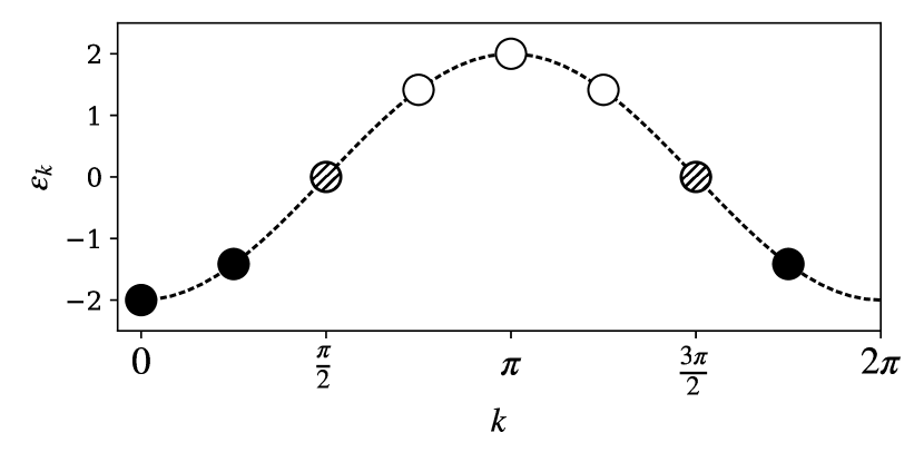
(a) $L=8$

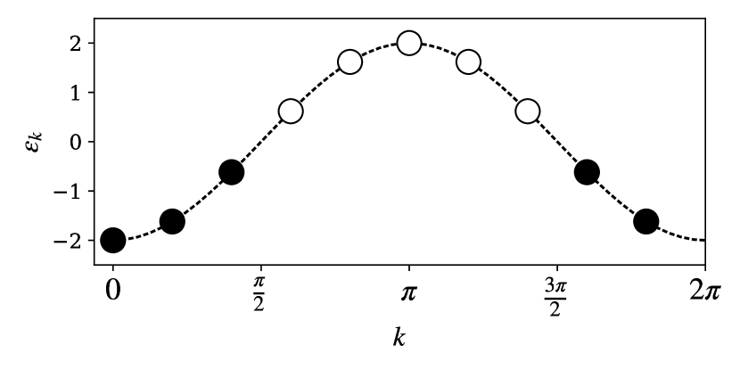
(b) $L=10$

Figure 19: Dispersion relation and energy levels of the half-filled tight binding model for (a) $L=8$ and (b) $L=10$. Solid black dots are occupied orbitals, blank circles are unoccupied orbitals, and circles with stripes are partially occupied orbitals due to degeneracy.

At finite temperature, we again evaluate the thermal average with thermal states. The matrix form of the phase operator $[\hat{Z}]$ based on the above discussion is:

$$\left[\hat{Z}\right]=\begin{bmatrix}0&0&0&\cdots&0&1\\ 1&0&0&\cdots&0&0\\ 0&1&0&\cdots&0&0\\ &&&\ddots&&\\ 0&0&0&\cdots&1&0\\ \end{bmatrix},$$ (112)

and the thermal operator of complex polarization has the form

$$\left[\bar{\hat{Z}}\right]=\begin{bmatrix}[\hat{Z}]&0\\ 0&\mathcal{I}\end{bmatrix}.$$ (113)

Since the Hamiltonian is diagonal with the basis $\{\psi_{k_{s}}\}$, the thermal density matrix has the form

$$\left[\bar{\hat{\rho}}\right]=\begin{bmatrix}\xi_{1}&&&&\\ &\xi_{2}&&&\\ &&\ddots&&\\ &&&\xi_{L}&\\ &&&&[\mathcal{I}]\end{bmatrix}.$$ (114)

The complex polarization can be evaluated according to Eq. (100),

$$Z_{N}(\beta)=\frac{1-(-1)^{L}\prod_{\mu}\xi_{\mu}}{\prod_{\mu}(1+\xi_{\mu})}$$ (115)

. Note that $\xi_{\mu}=e^{-\beta\varepsilon_{\mu}}>0$, so the denominator of Eq. (115) is always greater than zero.

Now let us examine two extreme cases: $\beta\rightarrow\infty$ (zero temperature) and $\beta\rightarrow 0$ (infinite temperature). At $\beta\rightarrow\infty$, if the Fermi level is above all bands, then $\xi_{\mu}\gg 1$ for all $\mu$, and Eq. (115) is well approximated by

$$|Z_{N}|\approx\frac{\prod_{\mu}\xi_{\mu}}{\prod_{\mu}\xi_{\mu}}=1.$$ (116)

Therefore the lattice is an insulator. However, when the Fermi level is below some bands (unoccupied orbitals), then the $\xi$ values of these bands $\rightarrow 0$, and the numerator of Eq. (115) $\rightarrow 1$, while the denominator $\prod_{\mu}(1+\xi_{\mu})\rightarrow\infty$, so $Z_{N}\rightarrow 0$, giving a conducting solution. The above low temperature limit agrees with the previous analysis of ground state metal-insulator transition of the tight binding model.

At $\beta\rightarrow\infty$, all $\xi_{\mu}\rightarrow 1$, resulting in an numerator $0$ ($L$ is even) or $2$ ($L$ is odd), while the denominator is $2^{L}$. Therefore, $Z_{N}\rightarrow 0$ as $L\rightarrow\infty$, and the electrons in the tight binding model are delocalized.

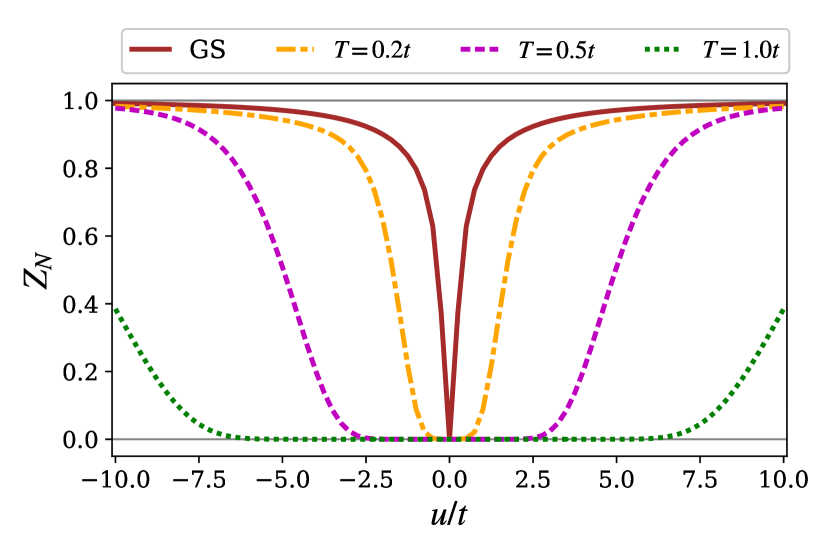
Figure 20: Complex polarization of the tight binding model ($L=42$) with staggered potential $u$ at ground state (GS), $T=0.2$, $T=0.5$, and $T=1.0$, respectively.

Next we add the staggered potential $u$ onto the original tight binding model:

$$\hat{h}=-t\sum_{\mu}\hat{a}^{{\dagger}}_{\mu}\hat{a}_{\mu+1}+\text{h.c.}+u\sum_{\mu\in\text{odd}}\hat{a}^{{\dagger}}_{\mu}\hat{a}_{\mu},$$ (117)

where $u>0$ is only applied to the odd sites. For simplicity, we assume that $L$ is even. The effect of $u$ is to provide a potential wall/well for every other site, and this effect prohibits the free flow of electrons. For the rest of the tight binding calculations, we choose the chain length $L=42$ and Boltzmann constant $k_{B}=1$, and use $t$ as the energy unit. In Fig. 20 we show the complex polarization $Z_{N}$ of the half-filled tight binding model against the staggered potential $u$ at ground state, $T=0.2t$, $T=0.5t$ and $T=1.0t$. As predicted above, the half-filled ground state of the original tight binding model ($u=0$) with $L=4m+2$ is metallic with $Z_{N}=0$. As the staggered potential turned on, ground state $Z_{N}$ grows rapidly and the system becomes more and more insulating. With raising the temperature, the metallic regime expands within the small $|u|$ region, and the growth curve of $Z_{N}$ with respect to $|u|$ becomes more flat. The temperature effect smears the sharp transition at ground state. Note that the curves are symmetric to $u=0$ since only the potential differences between adjacent sites affect the state of the system.

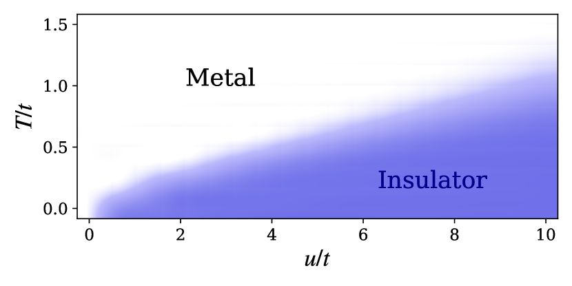
Figure 21: Phase diagram of the tight binding model ($L=42$) with the staggered potential $u$. The blue area corresponds to $Z_{N}>0$ (insulator) and the white area corresponds to $Z_{N}=0$ (metal). The 2D plot is smoothed by Bessel interpolation. Grid: $20$ points in the $x$-axis and $10$ points in the $y$-axis.

We show the phase diagram of $Z_{N}$ for the tight binding model with respect to the staggered potential $u$ and temperature $T$ in Fig. 21. We observed a sharp barrier between the metallic phase and insulating phase at $u\rightarrow 0_{+}$ and low temperature, and then the barrier becomes rather vague at larger $u$ with a higher transition temperature. This observation is consistent with the flatter curves at a higher temperature in Fig. 20. We further observe a linear growth of transition temperature $T_{c}$ with respect to $u$ at larger $u$. Since the transition temperature $T_{c}$ is directly related to the gap of the system, we also plotted the gap against $u$ in Fig. 22. The linear dependence of $\Delta_{\text{gap}}$ to the staggered potential $u$ at large $u$ region is consistant to the linear $T_{c}-u$ relationship in Fig. 21. At $u$ smaller than $0.1t$, we observe a rather slow growth of $\Delta_{\text{gap}}$ with $u$, which agrees with the metallic phase at $u\approx 0$ and then a sudden appearance of the insulator phase with a nearly verticle wall.

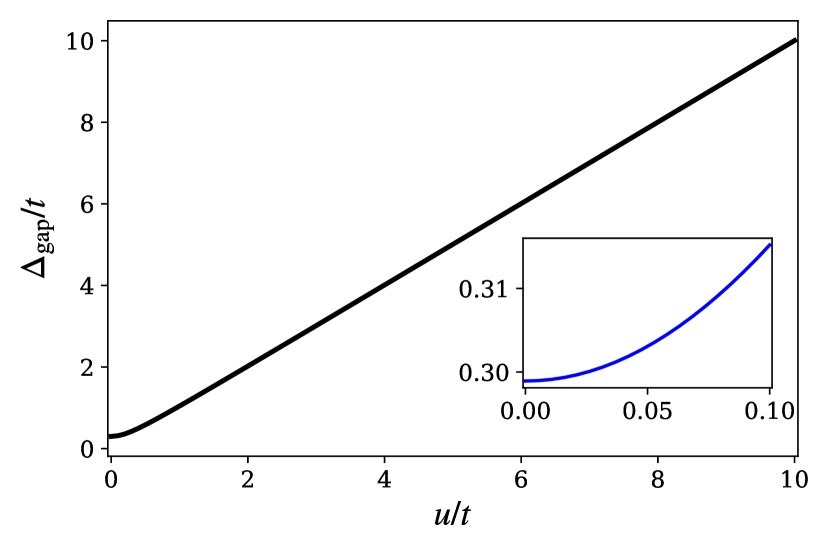
Figure 22: Energy gap of the half-filled staggered tight binding model against the staggered potential $u$. Inset: energy gap for $u\in[0t,0.1t]$.

18 Hydrogen chain

A linear chain of hydrogen atoms equispaced [97, 141, 99, 96, 101, 142] is the simplest ab initio periodic system that one can find. Unlike the simplicity of the structure, the phase diagram of the hydrogen chain involves complex components: metal-insulator transition (MIT), paramagnetic-antiferromagnetic (PM-AFM) transition and dimerization [12]. Hydrogen chain has a similar structure as the one-dimensional Hubbard model which has been studied for decades. Compared to the Hubbard model where electron-electron interactions are of short range, the Coulomb interaction in the hydrogen chain is long-ranged. Moreover, calculations beyond the minimal basis set (STO-6G) will introduce a multi-band effect into the hydrogen chain, which is absent in the one-band model systems.

In the following, we compute the complex polarization at both ground state and finite temperature for the hydrogen chain system with atoms equally spaced along the $z$-direction. The H-H bond length $R$ is introduced as the parameter and adjusted to show different phases. The Hamiltonian of this problem is

$$\hat{H}=-\frac{1}{2}\sum_{\mu=1}^{N}\nabla^{2}_{\mu}+\sum_{\mu<\nu}^{N}\frac{1}{|\mathbf{r}_{\mu}-\mathbf{r}_{\nu}|}-\sum_{\mu,a}^{N}\frac{1}{|\mathbf{r}_{\mu}-\mathbf{R}_{a}|}+\sum_{a<b}^{N}\frac{1}{|\mathbf{R}_{a}-\mathbf{R}_{b}|}$$ (118)

where $(\mathbf{r}_{1},...,\mathbf{r}_{N})$ are the electron positions in the Cartesian coordinates, $\mathbf{R}_{a}=aR\hat{\mathbf{e}}_{z}$ is the position of the $a$th atom on $z$-axis. In this work, energies and the temperature ($k_{B}=1$) are measured in Hartree ($me^{4}/\hbar^{2}$) and lengths in Bohr radius $a_{B}=\hbar^{2}/(me^{2})$. In one supercell, $30$ hydrogen atoms are included and only the $\Gamma$ point in the reciprocal space is taken into account. The basis set is 6-31G, where the 1$s$ orbital and the 2$s$ orbital are included. We evaluate the complex polarization $Z_{N}$, staggered magnetic moment $m$, electron population on 2s orbital, and the HOMO-LUMO gap of above hydrogen chain system at ground state, $T=0.01,0.02,0.03$ and $0.04$ Hartree. We present the results from unrestricted Hartree-Fock (UHF) and DFT (GGA/PBE and B3LYP) calculations in Fig. 23, Fig. 24, and Fig. 25. All calculations are performed within the framework of the quantum chemistry package PySCF [109, 110].

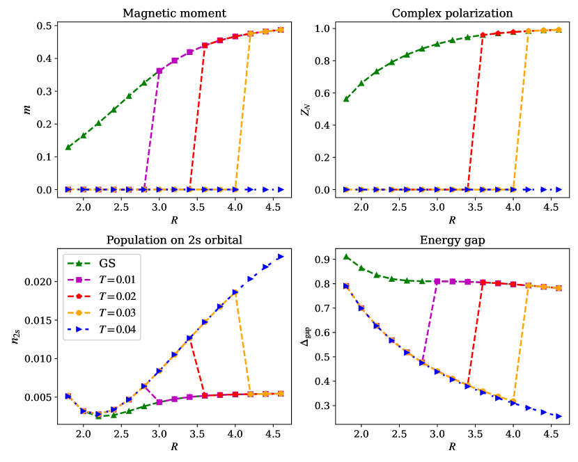
Figure 23: Complex polarization, magnetic moment, population on 2s orbital and energy gap of hydrogen chain with unrestricted Hartree-Fock method. Note that the complex polarization at $T=0.01$ is not presented here due to overflow.

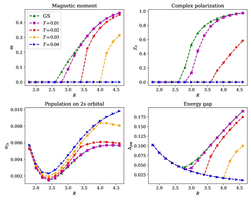
Figure 24: Complex polarization, magnetic moment, population on 2s orbital, and energy gap of hydrogen chain from DFT with PBE functional.

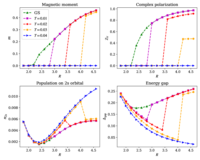
Figure 25: Complex polarization, magnetic moment, population on 2s orbital, and energy gap of hydrogen chain from DFT with B3LYP functional.

$T$/Hartree	Hartree-Fock	PBE	B3LYP
Ground state	$\sim$1.0	2.6	2.2
0.01	2.8	2.8	2.8
0.02	3.4	3.4	3.4
0.03	4.0	4.0	4.0

Table 1: PM-AFM transition bond length $R$ (in Bohr) at ground state and low temperature.

$T$/Hartree	Hartree-Fock	PBE	B3LYP
Ground state	$\sim$1.0	2.6	2.2
0.01	-	2.8	2.8
0.02	3.4	3.6	3.4
0.03	4.0	-	4.0

Table 2: Metal-insulator transition bond length $R$ (in Bohr) at ground state and low temperature.

All of the three methods predicted metal-insulator transition and PM-AFM transition at ground state and low temperature. The transition $R$ predicted by the above methods are summarized in Table 1 and Table 2. The two transitions happened nearly simultaneously, which provided evidence for the hypothesis that the insulator at large $R$ regime is an antiferromagnetic (AFM) insulator. With a metal to insulator transition happening with raising $R$, the population of the 2s orbital experienced a sudden drop, which indicates that the origin of the metal phase at small $R$ regime is caused by the crossover between 1$s$ and 2$s$ bands. Although the three methods all predicted the transitions, the behaviors of the order parameters against $R$ are quite different between UHF and PBE calculations. UHF predicted a much smaller transition $R$ at ground state ($\sim 1Bohr$), while PBE predicted $R_{c}$ to be $\sim 2.6Bohr$. The finite temperature predictions of $R_{c}$ for PM-AFM transitions from the two methods are similar, while the transition behaviors are quite different: UHF described that the finite temperature curves experienced a sudden jump from zero to the ground state curve; PBE predicted that the finite temperature curves grew from zero at $R_{c}$ and reached to a peak which decreases with temperature. Moreover, at $T=0.03$ and $R>4.0$, PBE predicted an AFM metal ($m>0$ and $Z_{N}=0$). This observation confirmed that the metal is mainly caused by the crossover of 1$s$ and 2$s$ bands, and the existence of the AFM order does not necessarily guarantee an insulating phase. However, the AFM metal phase is not observed with the other two methods. The B3LYP results in Fig. 25 are closer to those from UHF, except that the peaks of $m$ and $Z_{N}$ drop as the temperature increases.

19 Conclusion

In this chapter, we presented the finite temperature formulation of complex polarization under the scheme of thermal field theory. The complex polarization has a direct relationship with the electron localization at ground state: when the complex polarization is zero, the electrons are delocalized, and thus the system is metallic; when the complex polarization is nonzero, the electrons are localized and thus the system is insulating. At finite temperature, the complex polarization can also be used as the indicator of metal-insulator transition. We applied the thermofield implementation of the complex polarization to the tight binding model with staggered potential $u$, where as $u$ increases, the electrons tend to sit on the site with lower potential, and thus are localized. We observed the increase of the complex polarization with $u$ for both ground state and finite temperature. Moreover, we found that the transition temperature predicted by the complex polarization is linearly dependent on the staggered potential $u$ at intermediate to large $u$ regime, which is consistent with the linear dependence of the energy gap on $u$ at this intermediate to large $u$ regime. Therefore, the energy gap, electron localization, and complex polarization provide the same predictions of the metal-insulator transition behaviors. We further studied the metal-insulator and paramagnetic-antiferromagnetic (PM-AFM) transition for the hydrogen chain system by computing the complex polarization and magnetic moment against temperature and H-H bond length. Along with the results of the population of 2s orbitals and the energy gap, we confirmed that the origin of the metallic phase is the crossover of $1s$ and $2s$ (or higher, e.g, $2p$) bands. The antiferromagnetic (AFM) phase is usually accompanied by the insulating phase, but at finite temperature, we saw that PBE predicted an AFM metallic phase, which indicates that the disappearance of the insulating phase is not necessarily due to the loss of AFM phase. With complex polarization proving to be a good indicator of metal-insulator transition at both ground state and finite temperature, further applications are anticipated to bring more insights into this intriguing phenomena.

Chapter 5 Quantum imaginary time evolution and quantum thermal simulation

20 Abstract

An efficient way to compute Hamiltonian ground-states on a quantum computer stands to impact many problems in the physical and computer sciences, ranging from quantum simulation to machine learning. Unfortunately, existing techniques, such as phase estimation and variational algorithms, display potential disadvantages, such as requirements for deep circuits with ancillae and high-dimensional optimization. We describe the quantum imaginary time evolution and quantum Lanczos algorithms, analogs of classical algorithms for ground (and excited) states, but with exponentially reduced space and time requirements per iteration, and avoiding deep circuits with ancillae and high-dimensional optimization. We further discuss quantum imaginary time evolution as a natural subroutine to generate Gibbs averages through an analog of minimally entangled typical thermal states. We implement these algorithms with exact classical emulation as well as in prototype circuits on the Rigetti quantum virtual machine and Aspen-1 quantum processing unit, demonstrating the power of quantum elevations of classical algorithms.

21 Introduction

An important application for a quantum computer is to compute the ground-state $\Psi$ of a Hamiltonian $\hat{H}$ [143, 144, 145]. This arises in simulations, for example, of the electronic structure of molecules and materials [146, 147], as well as in optimization when the cost function is encoded in a Hamiltonian. While efficient ground-state determination cannot be guaranteed for all Hamiltonians, as this is a QMA complete problem [148], several heuristic quantum algorithms have been proposed, such as adiabatic state preparation with quantum phase estimation (QPE) [43, 44] and quantum-classical variational algorithms, including the quantum approximate optimization algorithm (QAOA) [45, 46, 47] and variational quantum eigensolver (VQE) [48, 49, 50]. While there have been many advances with these algorithms, they also have potential disadvantages, especially in the context of near-term quantum computing architectures and limited quantum resources. For example, phase estimation produces a nearly exact eigenstate, but appears impractical without error correction, while variational algorithms, although somewhat robust to coherent errors, are limited in accuracy for a fixed variational form, and involve a high-dimensional noisy classical optimization [149].

In classical simulations, different strategies are employed to numerically determine exact ground-states of Hamiltonians. One popular approach is imaginary-time evolution, which expresses the ground-state as the long-time limit of the imaginary-time Schrödinger equation $-\partial_{\beta}|\Phi(\beta)\rangle=\hat{H}|\Phi(\beta)\rangle$, $|\Psi\rangle=\lim_{\beta\to\infty}\frac{|\Phi(\beta)\rangle}{\|\Phi(\beta)\|}$ (for $\langle\Phi(0)|\Psi\rangle\neq 0$). Unlike variational algorithms with a fixed ansatz, imaginary-time evolution always converges to the ground-state (as distinguished from imaginary-time ansatz optimization, which can be trapped in local minima [150]). Another common exact algorithm is the iterative Lanczos algorithm [151, 152] and its variations. The Lanczos iteration constructs the Hamiltonian matrix $\mathbf{H}$ in a successively enlarged Krylov subspace $\{|\Phi\rangle,\hat{H}|\Phi\rangle,\hat{H}^{2}|\Phi\rangle\ldots\}$; diagonalizing $\mathbf{H}$ yields a variational estimate of the ground-state which tends to $|\Psi\rangle$ for a large number of iterations. For a Hamiltonian on $N$ qubits, the classical complexity of imaginary time evolution and the Lanczos algorithm scales as $\sim 2^{\mathcal{O}(N)}$ in space as well as time. The exponential space comes from storing $\Phi(\beta)$ or the Lanczos vector, while exponential time comes from the cost of Hamiltonian multiplication $\hat{H}|\Phi\rangle$, as well as, in principle, though not in practice, the $N$-dependence of the number of propagation steps and propagation time, or number of Lanczos iterations. Thus it is natural to consider quantum versions of these algorithms that can overcome the exponential bottlenecks.

In this work, we will describe the quantum imaginary time evolution (QITE) and the quantum Lanczos (QLanczos) algorithms to determine ground-states (as well as excited states in the case of QLanczos) on a quantum computer. Compared to their classical counterparts, these achieve an exponential reduction in space for a fixed number of propagation steps or number of iterations, and for a given iteration or time-step offer an exponential reduction in time. They also offer advantages over existing ground-state quantum algorithms; compared to quantum phase estimation, they do not require deep circuits, and compared to variational ground-state algorithms with a fixed ansatz, they are guaranteed to converge to the ground-state, avoiding non-linear optimization. A crucial component of our algorithms is the efficient implementation of the non-Hermitian operation of an imaginary time step propagation $e^{-{\Delta\tau}\hat{H}}$ (for small ${\Delta\tau}$), assuming a finite correlation length in the state. Non-Hermitian operations are not natural on a quantum computer and are usually achieved using ancillae and postselection. We will describe how to implement imaginary time evolution on a given state, without ancillae or postselection. The lack of ancillae and complex circuits make QITE and QLanczos potentially suitable for near-term quantum architectures. Using the QITE algorithm, we further show how we can sample from thermal (Gibbs) states, also without deep circuits or ancillae as is usually the case, via a quantum analog of the minimally entangled typical thermal states (QMETTS) algorithm [153, 154]. We demonstrate the algorithms on spin and fermionic Hamiltonians (short- and long-range spin and Hubbard models, MAXCUT optimization, and dihydrogen minimal molecular model) using exact classical emulation, and demonstrate proof-of-concept implementations on the Rigetti quantum virtual machine (QVM) and Aspen-1 quantum processing units (QPUs).

22 Quantum imaginary-time evolution

Define a geometric $k$-local Hamiltonian $\hat{H}=\sum_{m}\hat{h}_{m}$ (where each term $\hat{h}_{m}$ acts on at most $k$ neighbouring qubits on an underlying graph) and a Trotter decomposition of the corresponding imaginary-time evolution,

$$e^{-\beta\hat{H}}=(e^{-{\Delta\tau}\hat{h}_{1}}e^{-{\Delta\tau}\hat{h}_{2}}\ldots)^{n}+\mathcal{O}\left({{\Delta\tau}}\right);\ n=\frac{\beta}{{\Delta\tau}},$$ (119)

applied to a state $|\Psi\rangle$. After a single Trotter step, we have

$$|\Psi^{\prime}\rangle=e^{-{\Delta\tau}\hat{h}_{m}}|\Psi\rangle\quad.$$ (120)

The basic idea is that the normalized state $|\bar{\Psi}^{\prime}\rangle=|\Psi^{\prime}\rangle/\|\Psi^{\prime}\|$ can be generated from $|\Psi\rangle$ by a unitary operator $e^{-i{\Delta\tau}\hat{A}[m]}$ (which also depends on imaginary-time step) acting in the neighbourhood of the qubits acted on by $\hat{h}_{m}$, where the Hermitian operator $\hat{A}[m]$ can be determined from tomography of $|\Psi\rangle$ in this neighbourhood up to controllable errors. This is illustrated by the simple example where $|\Psi\rangle$ is a product state. Then, the squared norm $c=\|\Psi^{\prime}\|^{2}$ can be calculated from the expectation value of $\hat{h}_{m}$, which requires measurements over $k$ qubits,

$$c=\langle\Psi|e^{-2{\Delta\tau}\hat{h}[m]}|\Psi\rangle=1-2{\Delta\tau}\langle\Psi|\hat{h}_{m}|\Psi\rangle+\mathcal{O}({\Delta\tau}^{2}).$$ (121)

Because $|\Psi\rangle$ is a product state, $|\Psi^{\prime}\rangle$ is obtained by acting the unitary operator $e^{-i{\Delta\tau}\hat{A}[m]}$ also on $k$ qubits. $\hat{A}[m]$ can be expanded in terms of an operator basis, such as the Pauli basis $\{\sigma_{i}\}$ on $k$ qubits,

$$\hat{A}[m]=\sum_{i_{1}i_{2}\ldots i_{k}}a[m]_{i_{1}i_{2}\ldots i_{k}}\sigma_{i_{1}}\sigma_{i_{2}}\ldots\sigma_{i_{k}},$$ (122)

where $I$ denotes the index $i_{1}i_{2}\ldots i_{D}$. Then, up to $\mathcal{O}({\Delta\tau})$, the vector of coefficients $a[m]_{i_{1}i_{2}\ldots i_{k}}$ can be determined from the linear system

$$\mathbf{S}\mathbf{a}[m]=\mathbf{b},$$ (123)

where the elements of $\mathbf{S}$ and $\mathbf{b}$ are expectation values over $k$ qubits of $\Psi$, namely

$$S_{i_{1}i_{2}\ldots i_{k},i_{1}^{\prime}i_{2}^{\prime}\ldots i_{k}^{\prime}} =\langle\Psi|\sigma_{i_{1}}^{\dagger}\sigma_{i_{2}}^{\dagger}\ldots\sigma_{i_{k}}^{\dagger}\sigma_{i_{1}^{\prime}}\sigma_{i_{2}^{\prime}}{\color[rgb]{0,0,1}\dots}\sigma_{i_{k}^{\prime}}|\Psi\rangle$$

$$b_{i_{1}i_{2}\ldots i_{k}} =-i\,c^{-\frac{1}{2}}\,\langle\Psi|\sigma_{i_{1}}^{\dagger}\sigma_{i_{2}}^{\dagger}\ldots\sigma_{i_{k}}^{\dagger}\hat{h}[m]|\Psi\rangle.$$ (124)

In general, $\mathbf{S}$ will have a null space; to ensure $\mathbf{a}[m]$ is real, we minimize $\|c^{-1/2}\Psi^{\prime}-(1-i{\Delta\tau}\hat{A}[m])\Psi\|$ w.r.t. real variations in $\mathbf{a}[m]$. Note that the solution is determined from a linear problem, thus there are no local minima.

In this simple case, the normalized result of the imaginary time evolution step could be represented by a unitary over $k$ qubits, because $|\Psi\rangle$ had a zero correlation length. After the initial step, this is no longer the case. However, for a more general $|\Psi\rangle$ with finite correlation length extending over $C$ qubits (meaning that the correlations between two observables separated by distance $l$ are bounded by $\exp(-l/C)$), $|\Psi^{\prime}\rangle$ can be generated by a unitary acting on a domain of width $D:=\log(1/\delta)C$ qubits surrounding the qubits acted on by $h_{i}$ (this follows from Uhlmann’s theorem [155]; see Appendix for a proof), with $\delta$ the approximation error for that time step. The unitary $e^{-i{\Delta\tau}A[i]}$ can then be determined by measurements and solving the least squares problem over $D$ qubits. For example, if we consider a nearest-neighbor local Hamiltonian on a $d$-dimension square lattice, the number of qubits $D$ where the unitary acts is bounded by $(2\log(1/\delta)C)^{d}$. Because correlations are induced only by the gates applied at previous time steps, the correlation length increases at most with a velocity bounded by a constant $\alpha_{v}$ which depends on the geometry of the lattice and the locality of interactions. Consequently, each successive imaginary time step can be simulated by a unitary over an increasingly large neighborhood whose size propagates with velocity bounded by $\alpha_{v}$ (Fig. 1).

The number of measurements and classical storage at an imaginary time $\beta$ (starting the propagation from a product state) is bounded by $\exp(O((\alpha_{v}\beta)^{d}))$ for each unitary update, since each unitary at that level acts on at most $(2\alpha_{v}\beta)^{d}$ sites; classical solution of the least squares equation has the same scaling $\exp(O((\alpha_{v}\beta)^{d}))$, as does the synthesis and application of the unitary $e^{-i{\Delta\tau}A[i]}$. Thus, space and time requirements are bounded by exponentials of $\beta^{d}$, but are polynomial in $N$ (the polynomial in $N$ comes from the number of terms in $H$ and from the control of the Trotter error).

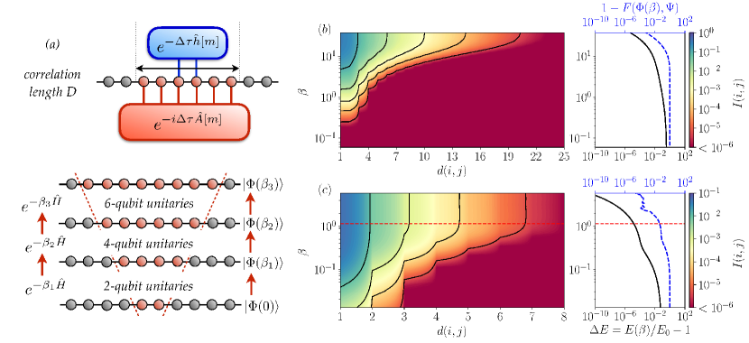
Figure 26: Quantum imaginary time evolution algorithm and correlation length. (a) Schematic of the QITE algorithm. Top: imaginary-time evolution under a geometric $k$-local operator $\hat{h}[m]$ can be reproduced by a unitary operation acting on a group of $D>k$ qubits. Bottom: exact imaginary-time evolution starting from a product state requires unitaries acting on a domain $D$ that grows with $\beta$. (b,c) Left: mutual information $I(i,j)$ between qubits $i$, $j$ as a function of distance $d(i,j)$ and imaginary time $\beta$, for a 1D (b) and a 2D (c) FM transverse-field Ising model, with $h=1.25$ (1D) and $h=3.5$ (2D). The mutual information is seen to saturate at longer times. Right: relative error in the energy $\Delta E$ and fidelity $F=|\langle\Phi(\beta)|\Psi\rangle|^{2}$ between the finite-time state $\Phi(\beta)$ and infinite-time state $\Psi$ as a function of imaginary time. The noise in the 2D fidelity error at large $\beta$ arises from the approximate nature of the algorithm used.

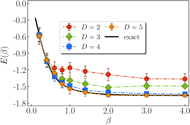
Figure 30: Thermal (Gibbs) average $\langle E\rangle$ at temperature $\beta$ from QMETTS for a 1D 6-site Heisenberg model (exact emulation).

Saturation of correlations. Note that the correlation volume cannot be larger than $N$. In many physical systems, we expect the correlation volume to increase with $\beta$ and saturate for $C^{d}\ll N$ [156]. As an example, in Fig. 26 we plot the mutual information between qubits $i$ and $j$ for the 1D and 2D FM transverse field Ising models computed by tensor network simulation which shows a monotonic increase and clear saturation. If saturation occurs before the ground-state is attained, the cost of the algorithm for subsequent time-steps becomes linear in $\beta$, and exponential in $C^{d}$.
Comparison to classical algorithm. Unlike classical imaginary time evolution, QITE is bounded by an exponential in $\beta$, rather than an exponential in $N$. Thus for fixed $\beta$ (and the same number of Trotter steps), we achieve an exponential reduction in cost in space and time in $N$ compared to the classical algorithm.
Comparison to tensor networks. If $|\Psi\rangle$ is represented by a tensor network in a classical simulation, then $e^{-{\Delta\tau}\hat{h}[m]}|\Psi\rangle$ can be obtained directly as a classical tensor network with an increased bond dimension [157, 158]. This bond dimension increases exponentially with imaginary time $\beta$, thus the storage of the tensors, as well as the cost of applying the imaginary time step $e^{-{\Delta\tau}\hat{h}[m]}$ to the tensors grows exponentially with $\beta$, similar to the quantum algorithm. The key distinction is that, other than in one dimension, we cannot guarantee that contracting the resulting classical tensor network to evaluate observables is efficient; it is a #P-hard problem in the worst case in two dimensions (and even in the average case for Gaussian distributed tensors) [159, 160]; no such problem exists in the quantum algorithm.
Fermionic Hamiltonians. For fermions, a non-local mapping to spins (e.g. through the Jordan-Wigner transformation) would violate the $k$-locality of the Hamiltonian. In principle, this can be bypassed by using a local mapping to spins [161]. Alternatively, we conjecture that by using a fermionic unitary, where the Pauli basis in Eq. (122) is replaced by the fermionic operator basis $\{1,\hat{a},\hat{a}^{\dagger},\hat{a}^{\dagger}\hat{a}\}$, the area of support for the fermionic unitary grows in the same fashion as the standard unitary for geometric $k$-local Hamiltonians described above. This can be tested in numerical simulations.
Long-range Hamiltonians. Consider a $k$-local Hamiltonian with long-range terms on a lattice, such as a general pairwise Hamiltonian. Then the action of $e^{-{\Delta\tau}\hat{h}[m]}$, if $\hat{h}[m]$ acts on qubits $i$ and $j$, can be emulated by a unitary constructed in the neighborhood of $i$ and $j$, over $(2C\log(1/\delta))^{k}$ sites.
Inexact time evolution. Given limited resources, we can choose to measure and construct the unitary over a reduced number of sites $D^{\prime}<D(\beta)$. For example, if $D^{\prime}=1$, this gives a mean-field approximation of the imaginary time evolution. While the unitary is no longer an exact representation of the imaginary time evolution, there is no issue of a local minimum in its construction, although the energy is no longer guaranteed to decrease in every time step. In this case, one might apply inexact imaginary time evolution simply until the energy stops decreasing. Alternatively, with limited resources, one may apply the quantum Lanczos algorithm described below.
Stabilization. Sampling noise in the expectation values of the Pauli operators can affect the solution to Eq. 123 that sometimes leads to numerical instabilities. We regularize $\mathbf{S}+\mathbf{S}^{T}$ against such statistical errors by adding a small $\delta$ to its diagonal. To generate the data presented in Fig. 29 and Fig. 30 of the main text, we used $\delta=0.01$ for 1-qubit calculations and $\delta=0.1$ for 2-qubits calculations.

23 Quantum Lanczos algorithm

Given the QITE subroutine, we now consider how to formulate a quantum version of the Lanczos algorithm. A significant practical motivation is that the Lanczos algorithm typically converges much more quickly than imaginary time evolution, and often in physical simulations only tens of iterations are needed to converge to good precision. In addition, Lanczos provides a natural way to compute excited states.

In quantum Lanczos, we generate a set of wavefunctions for different imaginary-time projections of an initial state $|\Psi\rangle$, using QITE as a subroutine. The normalized states are

$$|\Phi_{l}\rangle=\frac{e^{-l\Delta\tau\hat{H}}|\Psi_{T}\rangle}{\|e^{-l\Delta\tau\hat{H}}\Psi_{T}\|}\equiv n_{l}\,e^{-l\Delta\tau\hat{H}}|\Psi_{T}\rangle\quad 0\leq l<L_{\text{max}}\quad.$$ (125)

where $n_{l}$ is the normalization constant. For the exact imaginary-time evolution and $l$, $l^{\prime}$ both even (or odd) the matrix elements

$$S_{l,l^{\prime}}=\langle\Phi_{l}|\Phi_{l^{\prime}}\rangle\quad,\quad H_{l,l^{\prime}}=\langle\Phi_{l}|\hat{H}|\Phi_{l^{\prime}}\rangle$$ (126)

can be computed in terms of expectation values (i.e. experimentally accessible quantities) only. Indeed, defining $2r=l+l^{\prime}$, we have

$$S_{l,l^{\prime}}=n_{l}n_{l^{\prime}}\,\langle\Psi_{T}|e^{-l\Delta\tau\hat{H}}e^{-l^{\prime}\Delta\tau\hat{H}}|\Psi_{T}\rangle=\frac{n_{l}n_{l^{\prime}}}{n_{r}^{2}}\quad,$$ (127)

and similarly

$$H_{l,l^{\prime}}=n_{l}n_{l^{\prime}}\,\langle\Psi_{T}|e^{-l\Delta\tau\hat{H}}\hat{H}e^{-l^{\prime}\Delta\tau\hat{H}}|\Psi_{T}\rangle=\frac{n_{l}n_{l^{\prime}}}{n_{r}^{2}}\,\langle\Phi_{r}|\hat{H}|\Phi_{r}\rangle=S_{l,l^{\prime}}\,\langle\Phi_{r}|\hat{H}|\Phi_{r}\rangle\quad.$$ (128)

The quantities $n_{r}$ can be evaluated recursively, since

$$\frac{1}{n^{2}_{r+1}}=\langle\Psi_{T}|e^{-(r+1)\Delta\tau\hat{H}}e^{-(r+1)\Delta\tau\hat{H}}|\Psi_{T}\rangle=\frac{\langle\Phi_{r}|e^{-2\Delta\tau\hat{H}}|\Phi_{r}\rangle}{n_{r}^{2}}\quad.$$ (129)

For inexact time evolution, the quantities $n_{r}$ and $\langle\Phi_{r}|\hat{H}|\Phi_{r}\rangle$ can still be used to approximate $S_{l,l^{\prime}}$, $H_{l,l^{\prime}}$.

Given these matrices, we then solve the generalized eigenvalue equation $\mathbf{H}\mathbf{x}=E\mathbf{S}\mathbf{x}$ to find an approximation to the ground-state $|\Phi^{\prime}\rangle=\sum_{l}x_{l}|\Phi_{l}\rangle$ for the ground state of $\hat{H}$. This eigenvalue equation can be numerically ill-conditioned, as $S$ can contain small and negative eigenvalues for several reasons: (i) as $m$ increases the vectors $|\Phi_{l}\rangle$ become linearly dependent; (ii) simulations have finite precision and noise; (iii) $S$ and $H$ are computed approximately when inexact time evolution is performed.

To regularize the problem, out of the set of time-evolved states we extract a well-behaved sequence as follows: (i) start from $|\Phi_{\text{last}}\rangle=|\Phi_{0}\rangle$, (ii) add the next $|\Phi_{l}\rangle$ in the set of time-evolved states s.t. $|\langle\Phi_{l}|\Phi_{\text{last}}\rangle|<s$, where $s$ is a regularization parameter $0<s<1$, (iii) repeat, setting the $|\Phi_{\text{last}}\rangle=\Phi_{l}$ (obtained from (ii)), until the desired number of vectors is reached.

We then solve the generalized eigenvalue equation $\tilde{\mathbf{H}}\mathbf{x}=E\tilde{\mathbf{S}}\mathbf{x}$ spanned by this regularized sequence, removing any eigenvalues of $\tilde{\mathbf{S}}$ less than a threshold $\epsilon$. The QLanczos calculations reported in Fig. 27 (lower panel) of the main text were stabilized with this algorithm, in both cases using stabilization parameter $s=0.95$ and $\epsilon=10^{-14}$. The stabilization parameters used in the QLanczos calculations reported in Fig. 29 are $s=0.75$ and $\epsilon=10^{-2}$.

We demonstrate the QLanczos algorithm using classical emulation on the 1D Heisenberg Hamiltonian, as used for the QITE algorithm above in Fig. 27. Using exact QITE (large domains) to generate the matrix elements, quantum Lanczos converges much more rapidly than imaginary time evolution. Using inexact QITE (small domains), the convergence is usually faster and also reaches a lower energy. We also assess the feasibility of QLanczos in the presence of noise, using emulated noise on the Rigetti QVM as well as on the Rigetti Aspen-1 QPUs. In Fig. 29, we see that QLanczos also provides more rapid convergence than QITE with both noisy classical emulation as well as on the physical device for 1- and 2-qubits.

24 Quantum thermal averages

The QITE subroutine can be used in a range of other algorithms. As one example, we now discuss how to compute thermal averages of operators i.e. $\mathrm{Tr}\big{[}\hat{O}e^{-\beta\hat{H}}\big{]}/\mathrm{Tr}\big{[}e^{-\beta\hat{H}}\big{]}$ using imaginary time evolution. Several procedures have been proposed for quantum thermal averaging [162], ranging from generating the finite-temperature state explicitly with the help of ancillae, to a quantum analog of Metropolis sampling [163] that relies heavily on phase estimation. However, given a method for imaginary time evolution, one can generate thermal averages of observables without any ancillae or deep circuits. This can be done by adapting to the quantum setting the classical minimally entangled typical thermal state (METTS) algorithm [153, 154], which generates a Markov chain from which the thermal average can be sampled.

Consider the thermal average of an observable $\hat{O}$

$$\langle\hat{O}\rangle=\frac{1}{Z}\mathrm{Tr}[e^{-\beta\hat{H}}\hat{O}]=\frac{1}{Z}\sum_{i}\langle i|e^{-\beta\hat{H}/2}\hat{O}e^{-\beta\hat{H}/2}|i\rangle$$ (130)

where $\{|i\rangle\}$ is an orthonormal basis set, and $Z$ is the partition function. Defining $|\phi_{i}\rangle=P_{i}^{-1/2}e^{-\beta\hat{H}/2}|i\rangle$, we obtain

$$\langle\hat{O}\rangle=\frac{1}{Z}\sum_{i}P_{i}\langle\phi_{i}|\hat{O}|\phi_{i}\rangle$$ (131)

where $P_{i}=\langle i|e^{-\beta H}|i\rangle$. The summation in Eq.(131) can be estimated by sampling $|\phi_{i}\rangle$ with probability $P_{i}/Z$, and summing the sampled $\langle\phi_{i}|\hat{O}|\phi_{i}\rangle$.

In standard Metropolis sampling for thermal states, one starts from $|\phi_{i}\rangle$ and obtains the next state $|\phi_{j}\rangle$ from randomly proposing and accepting based an acceptance probability. However, rejecting and resetting in the quantum analog of Metropolis [163] is complicated to implement on a quantum computer, requiring deep circuits. The METTS algorithm provides an alternative way to sample $|\phi_{i}\rangle$ distributed with probability $P_{i}/Z$ without this complicated procedure. The algorithm is as follows

1. Choose a classical product state (PS) $|i\rangle$.

2. Compute $|\phi_{i}\rangle=P_{i}^{-1/2}e^{-\beta H/2}|i\rangle$ and calculate observables of interest.

3. Collapse $|\phi_{i}\rangle$ to a new PS $|i^{\prime}\rangle$ with probability $p(i\rightarrow i^{\prime})=|\langle i^{\prime}|\phi_{i}\rangle|^{2}$ and repeat Step 2.

In the above algorithm, $|\phi_{i}\rangle$ is named a minimally entangled typical thermal state (METTS). One can easily show that the set of METTS sampled following the above procedure has the correct Gibbs distribution [33]. Generally, $\{|i\rangle\}$ can be any orthonormal basis. For convenience when implementing METTS on a quantum computer, $\{|i\rangle\}$ are chosen to be product states.

On a quantum emulator or a quantum computer, the METTS algorithm is carried out as following

1. Prepare a product state $|i\rangle$.

2. Imaginary time evolve $|i\rangle$ with the QITE algorithm to $|\phi_{i}\rangle=P_{i}^{-1/2}e^{-\beta H/2}|i\rangle$, and measure the desired observables.

3. Collapse $|\phi_{i}\rangle$ to another product state by measurement.

In practice, to avoid long statistical correlations between samples, we used the strategy of collapsing METTS onto alternating basis sets [33]. For instance, for the odd METTS steps, $|\phi_{i}\rangle$ is collapsed onto the $X$-basis (assuming a $Z$ computational basis, tensor products of $|+\rangle$ and $|-\rangle$), and for the even METTS steps, $|\phi_{i}\rangle$ is collapsed onto the $Z$-basis (tensor products of $|0\rangle$ and $|1\rangle$). The statistical error is then estimated by block analysis [164]. In Fig. 30a we show the results of quantum METTS (using exact classical emulation) for the thermal average $\langle\hat{H}\rangle$ as a function of temperature $\beta$, for the 6-site 1D AFM transverse-field Ising model for several temperatures and domain sizes; sufficiently large $D$ converges to the exact thermal average at each $\beta$; error bars reflect only the finite samples in QMETTS. We also show an implementation of quantum METTS on the Aspen-1 QPU and QVM with a 1-qubit field model (Fig. 30b), and using the QVM for a 2-qubit AFM transverse field Ising model (Fig. 30d); while the noise introduces additional error including a systematic shift (Fig. 30c), the correct behaviour of the thermal average with temperature is reproduced on the emulated and actual quantum device.

25 Results

To illustrate the QITE algorithm, we have carried out exact classical emulations (assuming perfect expectation values and perfect gates) for several Hamiltonians: short-range 1D Heisenberg; 1D AFM transverse-field Ising; long-range 1D Heisenberg with spin-spin coupling $J_{ij}={|i-j|+1}^{-1};i\neq j$; 1D Hubbard at half-filling (mapped by Jordan-Wigner transformation to a spin model); a 6-qubit MAXCUT [45, 46, 47] instance, and a minimal basis 2-qubit dihydrogen molecular Hamiltonian [165]. We describe the models below.

1D Heisenberg and transverse field Ising model. The 1D short-range Heisenberg Hamiltonian is defined as

$$\hat{H}=\sum_{\langle ij\rangle}\hat{\mathbf{S}}_{i}\cdot\hat{\mathbf{S}}_{j}\quad,$$ (132)

the 1D long-range Heisenberg Hamiltonian as

$$\hat{H}=\sum_{i\neq j}\frac{1}{|i-j|+1}\,\hat{\mathbf{S}}_{i}\cdot\hat{\mathbf{S}}_{j}\quad,$$ (133)

and the AFM transverse-field Ising Hamiltonian as

$$\hat{H}=\sum_{\langle ij\rangle}\hat{{S}}^{z}_{i}\hat{{S}}^{z}_{j}+\sum_{i}h\hat{S}^{x}_{i}\quad.$$ (134)

1D Hubbard model. The 1D Hubbard Hamiltonian is defined as

$$\hat{H}=-\sum_{\langle ij\rangle\sigma}a^{\dagger}_{i\sigma}a_{j\sigma}+U\sum_{i}\hat{n}_{i\uparrow}\hat{n}_{i\downarrow}$$ (135)

where $\hat{n}_{i\sigma}=a^{\dagger}_{i\sigma}a_{i\sigma}$, $\sigma\in\{\uparrow,\downarrow\}$, and $\langle\cdot\rangle$ denotes summation over nearest-neighbors, here with open-boundary conditions. We label the $n$ lattice sites with an index $i=0\dots n-1$, and the $2n-1$ basis functions as $|\varphi_{0}\rangle=|0\uparrow\rangle$, $|\varphi_{1}\rangle=|0\downarrow\rangle$, $|\varphi_{2}\rangle=|1\uparrow\rangle$, $|\varphi_{3}\rangle=|1\downarrow\rangle$ $\dots$. Under Jordan-Wigner transformation, recalling that

$$\hat{n}_{p}=\frac{1-Z_{p}}{2}\quad,\quad\hat{a}^{\dagger}_{p}\hat{a}_{q}+\hat{a}^{\dagger}_{q}\hat{a}_{p}=\frac{X_{p}X_{q}\prod_{k=q+1}^{p-1}Z_{k}\left(1-Z_{p}Z_{q}\right)}{2}\quad,$$ (136)

with $p=0\dots 2n-2$ and $q<p$, the Hamiltonian takes the form

$$\hat{H}=-\sum_{p}\frac{X_{p}X_{p+2}Z_{p+1}\left(1-Z_{p}Z_{p+2}\right)}{2}+U\sum_{p\,\mathrm{even}}\frac{(1-Z_{2i})(1-Z_{2i+1})}{4}+\mu\sum_{p}\frac{(1-Z_{p})}{2}$$ (137)

H₂ molecule minimal basis model. We use the hydrogen molecule minimal basis model at the STO-6G level of theory. This is a common minimal model of hydrogen chains [166, 167] and has previously been studied in quantum simulations, for example in [165]. Given a molecular geometry (H-H distance $R$) we perform a restricted Hartree-Fock calculation and express the second-quantized Hamiltonian in the orthonormal basis of RHF molecular orbitals as [168]

$$\hat{H}=H_{0}+\sum_{pq}h_{pq}\hat{a}^{\dagger}_{p}\hat{a}_{q}+\frac{1}{2}\sum_{prqs}v_{prqs}\hat{a}^{\dagger}_{p}\hat{a}^{\dagger}_{q}\hat{a}_{s}\hat{a}_{r}$$ (138)

where $a^{\dagger}$, $a$ are fermionic creation and annihilation operators for the molecular orbitals. The Hamiltonian (138) is then encoded by a Bravyi-Kitaev transformation into the 2-qubit operator

$$\hat{H}=g_{0}I\otimes I+g_{1}Z\otimes I+g_{2}I\otimes Z+g_{3}Z\otimes Z+g_{4}X\otimes X+g_{5}Y\otimes Y\quad,$$ (139)

with coefficients $g_{i}$ given in Table I of [165].

MAXCUT Hamiltonian. The MAXCUT Hamiltonian encodes the solution of the MAXCUT problem. Given a graph $\Gamma=(V,E)$, where $V$ is a set of vertices and $E\subseteq V\times V$ is a set of links between vertices in $V$, a cut of $\Gamma$ is a subset $S\subseteq V$ of $V$. The MAXCUT problem consists in finding a cut $S$ that maximizes the number of edges between $S$ and $S^{c}$ (the complement of $S$). We denote the number of links in a given cut $S$ as $C(S)$. The MAXCUT problem can be formulated as a Hamiltonian ground-state problem, by (i) associating a qubit to every vertex in $V$, (ii) associating to every partition $S=$ an element of the computational basis (here assumed to be in the $z$ direction) of the form $|z_{0}\dots z_{n-1}\rangle$, where $z_{i}=1$ if $i\in S$ and $z_{i}=0$ if $i\in S^{c}$, and finding the minimal (most negative) eigenvalue of the $2$-local Hamiltonian

$$\hat{C}=-\sum_{(ij)\in E}\frac{1-\hat{S}^{z}_{i}\hat{S}^{z}_{j}}{2}\quad.$$ (140)

The spectrum of $\hat{C}$ is a subset of numbers $C\in\{0,1\dots|E|\}$.

To assess the feasibility of implementation on near-term quantum devices, we have also carried out noisy classical emulation (sampling expectation values and with an error model) using the Rigetti quantum virtual machine (QVM) and a physical simulation using the Rigetti Aspen-1 QPUs, for a single qubit field model ($2^{-1/2}(X+Z)$)[169] and a 1D AFM transverse-field Ising model. We carry out QITE using different fixed domain sizes $D$ for the unitary or fermionic unitary.

For quantum simulations, we used pyQuil, an open source Python library, to write quantum circuits that interface with both Rigetti’s quantum virtual machine (QVM) and the Aspen-1 quantum processing units (QPUs). pyQuil provides a way to include noise models in the QVM simulations. Readout error can be included in a high-level API provided in the package and is characterized by $p_{00}$ (the probability of reading $|0\rangle$ given that the qubit is in state $|0\rangle$) and $p_{11}$ (the probability of reading $|1\rangle$ given that the qubit is in state $|1\rangle$). Readout errors can be mitigated by estimating the relevant probabilities and correcting the estimated expectation values. We do so by using a high level API present in pyQuil.

A general noise model can be applied to a gate in the circuit by applying the appropriate Kraus maps. Included in the package is a high level API that applies the same decoherence error attributed to energy relaxation and dephasing to every gate in the circuit. This error channel is characterized by the relaxation time $T_{1}$ and coherence time $T_{2}$. We also include in our emulation our own high-level API that applies the same depolarizing noise channel to every single gate by using the appropriate Kraus maps. The depolarizing noise is characterized by $p_{1}$, the depolarizing probability for single-qubit gates and $p_{2}$, the depolarizing probability for two-qubit gates.

25.1 Benchmarks

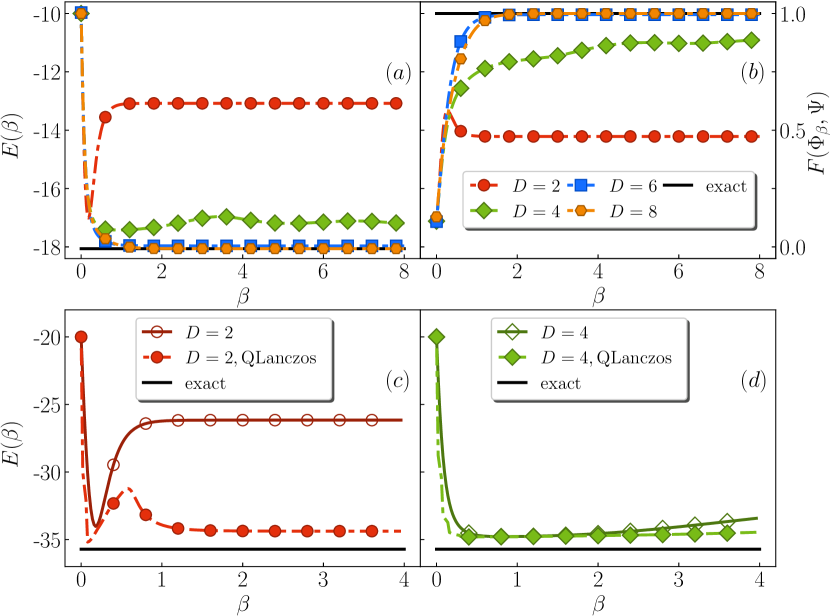
Figure 27: Energy calculations with QITE and QLanczos algorithms. Top: QITE energy $E(\beta)$ (a) and fidelity (b) between finite-time state $\Phi(\beta)$ and exact ground state $\Psi$ as function of imaginary time $\beta$, for a 1D 10-site Heisenberg model, showing the convergence with increasing unitary domains of $D=2-8$ qubits. Bottom: QITE (dashed red, dot-dashed green lines) and QLanczos (solid red, solid green lines) energies as function of imaginary time $\beta$, for a 1D Heisenberg model with $N=20$ qubits, using domains of $D=2$ (c) and $4$ qubits (d), showing improved convergence of QLanczos over QITE. Black line is the exact ground-state energy/fidelity.

Figs. 27 and 28 show the energy obtained by QITE as a function of $\beta$ and $D$ for the various models. As we increase $D$, the asymptotic ($\beta\to\infty$) energies rapidly converge to the exact ground-state. For small $D$, the inexact QITE tracks the exact QITE for a time until the correlation length exceeds $D$. Afterwards, it may go down or up. The non-monotonic behavior is strongest for small domains; in the MAXCUT example, the smallest domain $D=2$ gives an oscillating energy. In such cases, we consider a reasonable estimate of the ground-state energy to be the point at which the energy stops decreasing. In all models, increasing $D$ past a maximum value (less than $N$) no longer affects the asymptotic energy, showing that the correlations have saturated (this is true even in the MAXCUT instance).

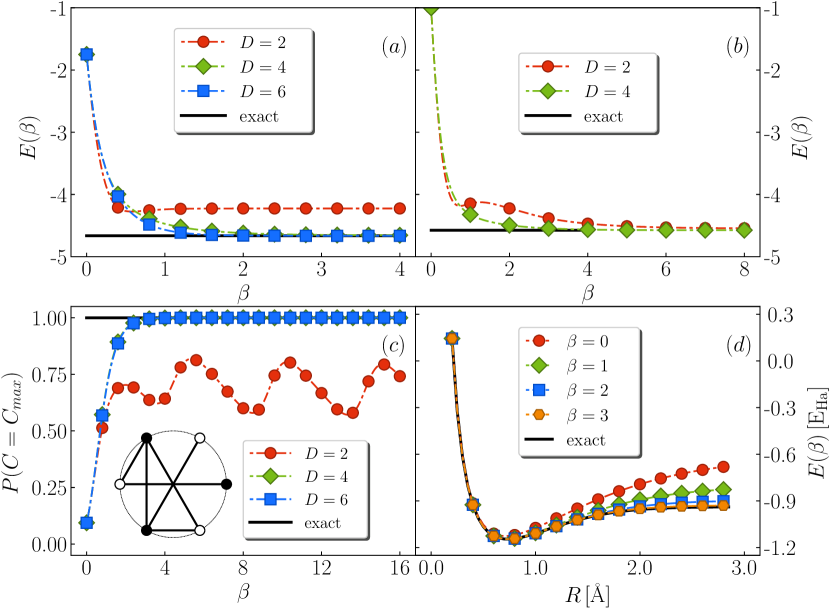
Figure 28: QITE energy evaluations. (a) QITE energy $E(\beta)$ as a function of imaginary time $\beta$ for a 6-site 1D long-range Heisenberg model, for unitary domains $D=2-6$; (b) a 4-site 1D Hubbard model with $U/t=1$, for unitary domains $D=2,4$; (d) the H₂ molecule in the STO-6G basis. (c) Probability of MAXCUT detection, $P(C=C_{max})$ as a function of imaginary time $\beta$, for the $6$-site graph in the panel. Black line is the exact ground-state energy/probability of detection.

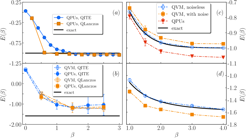
Figure 29: QITE, QLanczos, and QMETTS energies $E(\beta)$ as a function of imaginary time $\beta$ for 1-qubit field model using the QVM and QPU (qubit 14 on Aspen-1) and 2-qubit AFM transverse field Ising model using the QVM and QPU (qubit 14, 15 on Aspen-1). (a) Ground state energies for 1-qubit field model using the QVM and QPU (qubit 14 on Aspen-1); (b) ground state energies for 2-qubit AFM transverse field Ising model using the QVM and QPU (qubit 14, 15 on Aspen-1); (c) finite temperature energies for 1-qubit field model using the QVM and QPU (qubit 14 on Aspen-1) ; and (d) finite temperature energies for 2-qubit AFM transverse field Ising model using the QVM. Black lines are the exact solutions.

Figs. 29 shows the results of running the QITE algorithm on Rigetti’s QVM and Aspen-1 QPUs for 1- and 2- qubits, respectively. Encouragingly for near-term simulations, despite sampling errors and other errors such as gate, readout and incoherent errors present in the device, it is possible to converge to a ground-state energy close to the exact energy for the 1-qubit case. This result reflects a robustness that is sometimes informally observed in imaginary time evolution algorithms in which the ground state energy is approached even if the imaginary time step is not perfectly implemented. In the 2-qubit case, although the QITE energy converges, there is a systematic shift which is reproduced on the QVM using available noise parameters for readout, decoherence and depolarizing noise [170]. (Remaining discrepancies between the emulator and hardware are likely attributable to cross-talk between parallel gates not included in the noise model) . However, reducing decoherence and depolarizing errors in the QVM or using different sets of qubits with improved noise characteristics all lead to improved convergence to the exact ground-state energy.

26 Conclusions

. We have introduced quantum analogs of imaginary time evolution (QITE) and the Lanczos algorithm (QLanczos), that can be carried out without ancillae or deep circuits, and which achieve exponential reductions in space and time per iteration relative to their classical counterparts. They provide new quantum routes to approximate ground-states of Hamiltonians in both physical simulations and in optimization that avoid some of the disadvantages of phase estimation based approaches and variational algorithms. The QLanczos iteration appears especially powerful if sufficient sampling can be done, as in practice it obtains accurate estimates of ground-states from only a few iterations, and also provides an estimate of excited states. Additionally, further algorithms that use QITE and QLanczos as subroutines can be formulated, such as a quantum version of the METTS algorithm to compute thermal averages. Encouragingly, these algorithms appear useful in conjunction with near-term quantum architectures, and serve to demonstrate the power of quantum elevations of classical simulation techniques, in the continuing search for quantum supremacy.

Appendix A Appendix for Chapter 2 and Chapter 3

27 Proof of the finite temperature bath formula

Let $M$ be an arbitrary $N\times N$ full rank square matrix, and $Q_{k}$ be the $Q$ derived from the QR decomposition of the first $n$ columns of $M^{k}$, i.e., $M^{k}[:,:n]=Q_{k}R_{k}$, with $k=0,1,...,K$. Let $S$ ($|S|<N$) be a space spanned by $\{Q_{0},Q_{1},...,Q_{K}\}$, and $P$ be the projector onto $S$. The following equality holds

$$P^{\dagger}M^{l}P[:,:n]=(P^{\dagger}MP)^{l}[:,:n],\hskip 5.69046ptl\leq K+1.$$ (141)

We prove the statement by mathematical induction. First write $M$ in the following form

$$M=\begin{bmatrix}A&B\\ C&D\end{bmatrix},$$ (142)

where $A$ and $B$ are the first $n$ rows of $M$, $A$ and $C$ are the first $n$ columns of $M$. The projector has the form

$$P=\begin{bmatrix}I&0\\ 0&V\end{bmatrix},$$ (143)

where $I$ is an $n\times n$ matrix, and $V$ is an $(N-n)\times(K-1)n$ matrix with $(K-1)n<(N-n)$. The columns of $V$ are derived from the QR decomposition of $M^{k}[n:,:n]$, $k=1,...,K$ and then orthogonalized. We can write $V$ in the form

$$V=\begin{bmatrix}V_{1}&V_{2}&\cdots&V_{K}\end{bmatrix}$$ (144)

where $V_{k}$ is from the QR decomposition of $M^{k}[n:,:n]$. $\PP MP$ has the form

$$\PP MP=\begin{bmatrix}A&BV\\ \V C&\V DV\end{bmatrix}.$$ (145)

The mathematical induction consists of two parts:

(i) We start with $l=2$. The first $n$ columns of $P^{\dagger}M^{2}P$ and $(P^{\dagger}MP)^{2}$ are

$$\begin{split}P^{\dagger}M^{2}P[:,:n]&=\begin{bmatrix}A^{2}+BC\\ \V CA+\V DC\end{bmatrix}\\ (P^{\dagger}MP)^{2}[:,:n]&=\begin{bmatrix}A^{2}+BV\V C\\ \V CA+\V DV\V C\end{bmatrix}.\end{split}$$ (146)

The two are equal when

$$V\V C=V\V(VR)=VIR=VR=C$$ (147)

which is true since $V$ is the $Q_{1}$ from the QR decomposition of $C$. (Note that $\V V=I$, but $V\V\neq I$). Therefore, Eq. (141) holds for $l=2$ when $K\geq 1$.

(ii) Now let us inspect Eq. (141) for the $l$th order, assuming that Eq. (141) holds for the $(l-1)$th order, i.e. $\PP M^{l-1}P=(\PP MP)^{l-1}$. Let

$$M^{l-1}=\begin{bmatrix}W&X\\ Y&Z\\ \end{bmatrix}$$ (148)

and $M^{l}=MM^{l-1}$ has the form

$$M^{l}=\begin{bmatrix}AW+BY&AX+BZ\\ CW+DY&CX+DZ\end{bmatrix}$$ (149)

and

$$\PP M^{l-1}P=(\PP MP)^{l-1}=\begin{bmatrix}W&XV\\ \V Y&\V ZV\end{bmatrix}$$ (150)

One can prove that $CW$ and $C$ share the same $Q$ space from the QR decomposition: let $C=QR$, then $CW=QRW$, where $R$ and $W$ are square matrices; we then perform another QR decomposition of $RW$, $RW=U\tilde{R}$, where $U$ is a unitary matrix, then $CW=\tilde{Q}\tilde{R}$ with $\tilde{Q}=QU$. Therefore, $Q$ and $\tilde{Q}$ span the same space.

The first $n$ columns of $\PP M^{l}P$ and $(\PP MP)^{l}$ are

$$\PP M^{l}P[:,:n]=\begin{bmatrix}AW+BY\\ \V CW+\V DY\end{bmatrix},$$ (151)

$$\begin{split}(\PP MP)^{l}[:,:n]=&\left((\PP MP)(\PP MP)^{l-1}\right)[:,:n]\\ =&\begin{bmatrix}AW+BV\V Y\\ \V CW+\V DV\V Y\end{bmatrix}.\end{split}$$ (152)

Since $V$ contains $V_{l-1}$, which is derived from the QR decomposition of $Y$, we have $V\V Y=Y$ as in Eq. (147).

Combining (i) and (ii) we then see that Eq. (141) holds for the $l$th order with $K\geq l-1$ for $\forall l$.

28 Analytic gradient of the cost function for correlation potential fitting in DMET at finite temperature

We rewrite the gradient of the cost function Eq. (37) here

$$\frac{\mathrm{d}f}{\mathrm{d}u_{kl}}=\sum_{i,j\in\text{imp}}2(D_{ij}^{\text{low}}-D_{ij}^{\text{high}})\frac{\mathrm{d}D_{ij}^{\text{low}}}{\mathrm{d}u_{kl}},$$ (153)

where $D^{\text{low}}$ is the single-particle density matrix from the mean-field (low-level) calculations, $D^{\text{high}}$ is the high-level single partile density matrix, and $u$ is the correlation potential matrix. The key to evaluate Eq. (153) is to calculate $\frac{\mathrm{d}D_{ij}^{\text{low}}}{\mathrm{d}u_{kl}}$. For simplicity, we will drop the superscript on $D^{\text{low}}$.

At finite temperature, $D$ is given by

$$D=\frac{1}{1+e^{\beta(h-\mu+\delta u}},$$ (154)

where $h$ is the one-body Hamiltonian, $\mu$ is the chemical potential (Fermi level), and $\delta u$ is a small perturbation added to the Hamiltonian. Then $\frac{\mathrm{d}D_{ij}^{\text{low}}}{\mathrm{d}u_{kl}}$ has two parts:

$$\frac{\mathrm{d}D_{ij}(u,\mu(u))}{\mathrm{d}u_{kl}}=\frac{\partial D_{ij}}{\partial u_{kl}}\biggr{|}_{\mu}+\frac{\partial D_{ij}}{\partial\mu}\frac{\partial\mu}{\partial u_{kl}},$$ (155)

where the second part comes from the change of Fermi level due to the change of correlation potential.

The first part of Eq. (155) is evaluated by

$$\frac{\partial D_{ij}}{\partial u_{kl}}=\sum_{pq}C_{ip}C^{*}_{kp}K_{pq}C_{lq}C_{jq}^{*},$$ (156)

where $C$ is the molecular orbital (MO) coefficient matrix with $ijkl$ the site indices and $pq$ the MO indices, and

$$K_{pq}=n_{p}(1-n_{q})\frac{1-e^{\beta(\varepsilon_{p}-\varepsilon_{q})}}{\varepsilon_{p}-\varepsilon_{q}},$$ (157)

where $n_{p}$ is the occupation number on the $p$th orbital and $\varepsilon_{p}$ is the energy of $p$th orbital. Note that when $\varepsilon_{p}=\varepsilon_{q}$, both the denominator and numerator goes to zero and the value of $K_{pq}$ depends on $\beta$. When $\beta=\inf$, $\varepsilon_{p}=\varepsilon_{q}$ means $n_{p}=n_{q}=0$ or $1$, so $K_{pq}=0$ is bounded.

The second part is evaluated by

$$\begin{split}\frac{\partial D_{ij}}{\partial\mu}&=\sum_{p}\beta C_{ip}n_{p}(1-n_{p})C^{*}_{jp}\\ \frac{\partial\mu}{\partial u_{kl}}&=\frac{\sum_{p}n_{p}(1-n_{p})C_{kp}^{*}C_{lp}}{\sum_{p}n_{p}(1-n_{p})}.\end{split}$$ (158)

The contribution of this part is usually small at low temperature and becomes non-neglegible at higher temperature.

29 Davidson diagonalization

The Davidson diagonalization [18] algorithm is an efficient way to find the lowest/highest eigenvalues of a Hermitian matrix. In quantum chemistry, this method is widely used to get the ground state or low-lying excited states. This method constructs a subspace of the Hilbert space from an initial vector as the guess of the ground state, and diagonalize the Hamiltonian in this subspace. A preconditioner is used to make the algorithm more stable and converge fast. The steps to evaluate $m$ lowest eigenvectors are listed below:

1. Select initial guess vectors $\mathbf{v}^{i},i=1,...,n\geq m$ to form a subspace $\mathcal{S}$.

2. Construct the matrix representation of the Hamiltonian in the subspace $\mathcal{S}$: $\tilde{H}_{ij}=\mathbf{v}_{i}^{\dagger}\tilde{H}\mathbf{v}_{j}$.

3. Diagonalize $\tilde{H}$ to obtain the lowest $m$ eigenvalues and corresponding eigenvectors, $\tilde{H}\mathbf{x}^{p}=\lambda_{p}\mathbf{x}^{p}$. The current approximated eigenvectors are $\mathbf{c}_{p}=\sum_{i}x^{p}_{i}\mathbf{v}_{i}$.

4. Starting from the ground state ($p=1$), compute the residual vector $\mathbf{r}_{r}=\sum_{i=1}^{p}\left(H-\lambda_{i}\right)\mathbf{c}_{i}$. If $||\mathbf{r_{p}}||<\epsilon$, then move on to the next excited state ($p\rightarrow p+1$). Otherwise, compute the rescaled correction vector $\mathbf{\sigma}^{k}_{i}=\left(\lambda_{k}-A_{ii}\right)r^{k}_{i}$.

5. Orthogonalize $\mathbf{\sigma}^{k}$ with respect to $\mathcal{S}$ and normalize it. Add $\mathbf{\sigma}^{k}$ to $\mathcal{S}$. If the size of $\mathcal{S}$ exceeds the preset maximum size, discard the earlest vectors.

6. Go back to Step 2 until the algorithm converges.

The above algorithm iteratively finds the lowest $m$ eigenvectors of the Hamiltonian. Compared to other subspace methods such as Lanczos algorithm mentioned in Chapter 1, the Davidson algorithm is more accurate for both ground state and low-lying excited states. Note that when updating the excited state, the already converged ground state might be perturbed, therefore in Step 4, we recommend that one should always start from calculating the residual of the ground state. To make the algorithm faster, one could not worry about the ground state for a moment until all $m$ eigenvectors are derived, and then reexamine the residual of the ground state to make sure it is not perturbed.

Appendix B Appendix for Chapter 5

30 Representing imaginary-time evolution by unitary maps

As discussed in the main text, we map the scaled non-unitary action of $e^{-\Delta\tau\hat{h}_{m}}$ on a state $\Psi$ to that of a unitary $e^{-i\Delta\tau\hat{A}[m]}$, i.e.

$$|\Psi^{\prime}\rangle\equiv c^{-1/2}\,e^{-\Delta\tau\hat{h}_{m}}|\Psi\rangle=e^{-i\Delta\tau\hat{A}[m]}|\Psi\rangle\quad.$$ (159)

where $c=\langle\Psi|e^{-2\Delta\tau\hat{h}_{m}}|\Psi\rangle$. $\hat{h}_{m}$ acts on $k$ geometrically local qubits; $\hat{A}$ is Hermitian and acts on a domain of $D$ qubits around the support of $\hat{h}_{m}$, and is expanded as a sum of Pauli strings acting on the $D$ qubits,

$$\hat{A}[m] =\sum_{i_{1}i_{2}\ldots i_{D}}a[m]_{i_{1}i_{2}\ldots i_{D}}\sigma_{i_{1}}\sigma_{i_{2}}\ldots\sigma_{i_{D}}$$

$$=\sum_{I}a[m]_{I}\sigma_{I}$$ (160)

where $I$ denotes the index $i_{1}i_{2}\ldots i_{D}$. Define $|\Delta_{0}\rangle=\frac{|\Psi^{\prime}\rangle-|\Psi\rangle}{\Delta\tau}$ and $|\Delta\rangle=-i\hat{A}[m]|\Psi\rangle$. Our goal is to minimize the difference $||\Delta_{0}-\Delta||$. If the unitary $e^{-i\Delta\tau\hat{A}[m]}$ is defined over a sufficiently large domain $D$, then this error minimizes at $\sim 0$, for small $\Delta\tau$. Minimizing for real $a[m]$ corresponds to minimizing the quadratic function $f(a[m])$

$$f(a[m])=f_{0}+\sum_{I}b_{I}a[m]_{I}+\sum_{IJ}a[m]_{I}S_{IJ}a[m]_{J}$$ (161)

where

$$f_{0} =\langle\Delta_{0}|\Delta_{0}\rangle\quad,$$ (162)

$$S_{IJ} =\langle\Psi|\sigma^{\dagger}_{I}\sigma_{J}|\Psi\rangle\quad,$$ (163)

$$b_{I} =i\,\langle\Psi|\sigma^{\dagger}_{I}|\Delta_{0}\rangle-i\,\langle\Delta_{0}|\sigma_{I}|\Psi\rangle\quad,$$ (164)

whose minimum obtains at the solution of the linear equation

$$\left(\mathbf{S}+\mathbf{S}^{T}\right)\mathbf{a}[m]=-\mathbf{b}$$ (165)

In general, $\mathbf{S}+\mathbf{S}^{T}$ may have a non-zero null-space. Thus, we solve Eq. (165) either by applying the generalized inverse of $\mathbf{S}+\mathbf{S}^{T}$ or by an iterative algorithm such as conjugate gradient.

For fermionic Hamiltonians, we replace the Pauli operators in Eq. (160) by fermionic field operators. For a number conserving Hamiltonian, such as the fermionic Hubbard Hamiltonian treated in Fig. 3 in the main text, we write

$$\hat{A}[m] =\sum_{i_{1}i_{2}\ldots i_{D}}a[m]_{i_{1}i_{2}\ldots i_{D}}\hat{f}^{\dagger}_{i_{1}}\ldots\hat{f}^{\dagger}_{i_{D/2}}\hat{f}_{i_{D/2+1}}\ldots\hat{f}_{i_{D}}$$ (166)

where $\hat{f}^{\dagger}$, $\hat{f}$ are fermionic creation, annihilation operators respectively.

31 Proof of correctness from finite correlation Length

Here we present a more detailed analysis of the running time of the algorithm. Consider a $k$-local Hamiltonian

$$H=\sum_{l=1}^{m}h_{l}$$ (167)

acting on a $d$-dimensional lattice with $\|h_{i}\|\leq 1$, where $\|*\|$ is the operator norm. In imaginary time evolution (used e.g. in Quantum Monte-Carlo or in tensor network simulations) one typically applies Trotter formulae to approximate

$$\frac{e^{-\beta H}|\Psi_{0}\rangle}{\|e^{-\beta H}|\Psi_{0}\rangle\|}$$ (168)

for an initial state $|\Psi_{0}\rangle$ (which we assume to be a product state) by

$$\frac{\left(e^{-th_{1}/n}\ldots e^{-th_{m}/n}\right)^{n}|\Psi_{0}\rangle}{\|\left(e^{-th_{1}/l}\ldots e^{-th_{m}/n}\right)^{n}|\Psi_{0}\rangle\|}.$$ (169)

This approximation leads to an error which can be made as small as one wishes by increasing the number of time steps $n$.

Let $|\Psi_{s}\rangle$ be the state (after renormalization) obtained by applying $s$ terms $e^{-th_{i}/n}$ from $\left(e^{-th_{1}/n}\ldots e^{-th_{m}/n}\right)^{n}$; with this notation $|\Psi_{mn}\rangle$ is the state given by Eq. (169). In the QITE algorithm, instead of applying each of the operators $e^{-th_{i}/n}$ to $|\Psi_{0}\rangle$ (and renormalizing the state), one applies local unitaries $U_{s}$ which should approximate the action of the original operator. Let $|\Phi_{s}\rangle$ be the state after $s$ unitaries have been applied.

Let $C$ be an upper bound on the correlation length of $|\Psi_{s}\rangle$ for every $s$: we assume that for every $s$, and every observables $A$ and $B$ separated by $\text{dist}(A,B)$ sites,

$$\langle\Psi_{s}|A\otimes B|\Psi_{s}\rangle-\langle\Psi_{s}|A|\Psi_{s}\rangle\langle\Psi_{s}|B|\Psi_{s}\rangle\leq\|A\|\|B\|e^{-\text{dist}(A,B)/C}.$$ (170)

Theorem 1.

For every $\varepsilon>0$, there are unitaries $U_{s}$ each acting on

$$k(2C)^{d}\ln^{d}(2\sqrt{2}nm\varepsilon^{-1})$$ (171)

qubits such that

$$\left\||\Psi_{mn}\rangle-|\Phi_{mn}\rangle\right\|\leq\varepsilon$$ (172)

Proof.

We have

$$\left\||\Psi_{s}\rangle-|\Phi_{s}\rangle\right\| = \left\||\Psi_{s}\rangle-U_{s}|\Phi_{s-1}\rangle\right\|$$ (173)

$$\leq \left\||\Psi_{s}\rangle-U_{s}|\Psi_{s-1}\rangle\right\|+\left\||\Psi_{s-1}\rangle-|\Phi_{s-1}\rangle\right\|$$

To bound the first term we use our assumption that the correlation length of $|\Psi_{s-1}\rangle$ is smaller than $C$. Consider a region $R_{v}$ of all sites that are at most a distance $v$ (in the Manhattan distance on the lattice) of the sites in which $h_{i_{s}}$ acts. Let $\text{tr}_{\backslash R_{v}}(|\Psi_{s}\rangle\langle\Psi_{s}|)$ be the reduced state on $R_{v}$, obtained by partial tracing over the complement of $R_{v}$ in the lattice. Since

$$|\Psi_{s}\rangle=\frac{e^{-\beta h_{i_{s}}/n}|\Psi_{s-1}\rangle}{\|e^{-\beta h_{i_{s}}/n}|\Psi_{s-1}\rangle\|},$$ (174)

it follows from Eq. (170) and Lemma 9 of [171] that

$$\left\|\text{tr}_{\backslash R_{v}}(|\Psi_{s}\rangle\langle\Psi_{s}|)-\text{tr}_{\backslash R_{v}}(|\Psi_{s-1}\rangle\langle\Psi_{s-1}|)\right\|_{1}\leq\|e^{h_{i_{s}}/n}\|^{-1}e^{-\frac{v}{C}}\leq 2e^{-\frac{v}{C}},$$ (175)

where we used that for $n\geq 2\beta$, $\|e^{-\beta h_{i_{s}}/n}\|\geq\|I-\beta h_{i_{s}}/n\|\geq 1-\beta/n\geq 1/2$. Above $\|*\|_{1}$ is the trace norm.

The key result in our analysis is Uhlmann’s theorem (see e.g. Lemmas 11 and 12 of [171]). It says that two pure states with nearby marginals must be related by a unitary on the purifying system. In more detail, if $|\eta\rangle_{AB}$ and $|\nu\rangle_{AB}$ are two states s.t. $\|\eta_{A}-\nu_{A}\|_{1}\leq\delta$, then there exists a unitary $V$ acting on $B$ s.t.

$$\||\eta\rangle_{AB}-(I\otimes V)|\nu\rangle_{AB}\|\leq 2\sqrt{\delta}.$$ (176)

Applying Uhlmann’s theorem to $|\Psi_{s}\rangle$ and $|\Psi_{s-1}\rangle$, with $B=R_{v}$, and using Eq. (175), we find that there exists a unitary $U_{s}$ acting on $R_{v}$ s.t.

$$\left\||\Psi_{s}\rangle-U_{s}|\Psi_{s-1}\rangle\right\|\leq 2\sqrt{2}e^{-\frac{v}{2C}},$$ (177)

which by Eq. (173) implies

$$\left\||\Psi_{s}\rangle-U_{s}|\Psi_{s-1}\rangle\right\|\leq 2\sqrt{2}mne^{-\frac{v}{2C}},$$ (178)

Choosing $\nu=2C\ln(2\sqrt{2}nm\varepsilon^{-1})$ as the width of the support of the approximating unitaries, the error term above is $\varepsilon$. The support of the local unitaries is $k\nu^{d}$ qubits (as this is an upper bound on the number of qubits in $R_{d}$). Therefore each unitary $U_{s}$ acts on at most

$$k(2C)^{d}\ln^{d}(2\sqrt{2}nm\varepsilon^{-1})$$ (179)

qubits.

∎

Finding $U_{s}$: In the algorithm we claim that we can find the unitaries $U_{s}$ by solving a least-square problem. This is indeed the case if we can write them as $U_{s}=e^{iA[s]/n}$ with $A[s]$ a Hamiltonian of constant norm. Then for sufficiently large $l$, $U_{s}=I+iA[s]/n+O((1/n)^{2})$ and we can find $A[s]$ by performing tomography of the reduced state over the region where $U_{s}$ acts and solving the linear problem given in the main text. Because we apply Uhlmann’s Theorem to $|\Psi_{s-1}\rangle$ and

$$\frac{e^{-\beta h_{i_{s}}/n}|\Psi_{s-1}\rangle}{\|e^{-\beta h_{i_{s}}/n}|\Psi_{s-1}\rangle\|},$$ (180)

using $e^{-\beta h_{i_{s}}/n}=I-\beta h_{i_{s}}/n+O((1/n)^{2})$ and following the proof of the Uhlmann’s Theorem, we find that the unitary can indeed be taken to be close to the identity, i.e. $U_{s}$ can be written as $e^{iA[s]/n}$

Total Running Time: Theorem 1 gives an upper bound on the maximum support of the unitaries needed for a Trotter update, while tomography of local reduced density matrices gives a way to find the unitaries. The cost for tomography is quadratic in the dimension of the region, so it scales as $\exp(O(k(2C)^{d}\ln^{d}(2\sqrt{2}nm\varepsilon^{-1})))$. This is also the cost to solve classically the linear system which gives the associated Hamiltonian $A[s]$ and of finding a circuit decomposition of $U_{s}=e^{iA[s]/n}$ in terms of two qubit gates. As this is repeated $mn$ times, for each of the $mn$ terms of the Trotter decomposition, the total running time (of both quantum and classical parts) is

$$ml\exp(O(k(2C)^{d}\ln^{d}(2\sqrt{2}nm\varepsilon^{-1}))).$$ (181)

This is exponential in $(C)^{d}$, with $C$ the correlation length, and quasi-polynomial in $n$ (the number of Trotter steps) and $m$ (the number of local terms in the Hamiltonian. Note that typically $m=O(N)$, with $N$ the number of sites). While this an exponential improvement over the $\exp(O(N))$ scaling classically, the quasi-polynomial dependence on $m$ is still prohibitive in practice. Below we show how to improve on that.

Local Approximation: We expect in practice to substantially beat the bound on the support of the unitaries given in Theorem 1 above. Indeed, if one is only interested in a local approximation of the state (meaning that all the local marginals of $|\Phi_{nm}\rangle$ are close to the ones of $e^{-\beta H}|\Psi_{0}\rangle$, but not necessarily the global states), then we expect the support of the unitaries to be independent of the number of terms of the Hamiltonian $m$ (while for global approximation we get a polylogarithmic dependence on $m$).

The scaling with $m$ in the bound comes from the additive accumulation of error from each of the $ml$ steps (Eq. (173)). The assumption of a correlation length $C$ ensures that the errors of replacing each local term in the Trotter decomposition by a unitary do not all add up if one is interested in local observables. Indeed, the contribution of the local error for a region $S$ from the replacement of $e^{-\beta h_{j_{s}}/n}$ by $U_{s}$ is $\exp(-l/C)$, with $l$ the distance of the support of $h_{j_{s}}$ to $S$. Then we can substitute Eq. (175) by

$$\left\|\text{tr}_{\backslash S}(|\Psi_{mn}\rangle\langle\Psi_{mn}|)-\text{tr}_{\backslash S}(|\Phi_{mn}\rangle\langle\Phi_{mn}|)\right\|\leq 2\sqrt{2}n(C+|S|)e^{-\frac{v}{2C}}.$$ (182)

with $|S|$ the size of the support of $S$. This gives a bound on the size of the support of the unitaries $U_{s}$ of

$$k(2C)^{d}\ln^{d}(2\sqrt{2}n(C+|S|)\varepsilon^{-1})$$ (183)

Using this improved bound, the total running time becomes

$$ml\exp(O(k(2C)^{d}\ln^{d}(2\sqrt{2}n(C+|S|)\varepsilon^{-1}))).$$ (184)

As $m=O(N)$, we find the scaling with the number of sites $N$ to be linear.

Non-Local Terms: Suppose the Hamiltonian has a term $h_{q}$ acting on qubits which are not nearby, e.g. on two sites $i$ and $j$. Then $e^{-\beta h_{q}/n}$ can still be replaced by an unitary, which only acts on sites $i$ and $j$ and qubits in the neighborhoods of the two sites. This is the case if we assume that the state has a finite correlation length and the proof is again an application of Uhlmann’s theorem (we follow the same argument from the proof of Theorem 1 but define $R_{v}$ in that case as the union of the neighborhoods of $i$ and $j$). Note however that the assumption of a finite correlation length might be less natural for models with long range interactions.

32 Spreading of correlations

In the main text, we argued that the correlation volume $V$ of the state $e^{-\beta H}|\Psi\rangle$ is bounded for many physical Hamiltonians and saturates at the ground-state with $V\ll N$ where $N$ is the system size. To numerically measure correlations, we use the mutual information between two sites, defined as

$$I(i,j)=S(i)+S(j)-S(i,j)$$ (185)

where $S(i)$ is the von Neumann entropy of the density matrix of site $i$ ($\rho(i)$) and similarly for $S(j)$, and $S(i,j)$ is the von Neumann entropy of the two-site density matrix for sites $i$ and $j$ ($\rho(i,j)$).

To compute the mutual information in Fig. 1 in the main text, we used matrix product state (MPS) and finite projected entangled pair state (PEPS) imaginary time evolution for the spin-$1/2$ 1D and 2D FM transverse field Ising model (TFI)

$$H_{TFI}=-\sum_{\langle ij\rangle}\sigma^{z}_{i}\sigma^{z}_{j}-h\sum_{i}\sigma^{x}_{i}$$ (186)

where the sum over $\langle i,j\rangle$ pairs are over nearest neighbors. We use the parameter $h=1.25$ for the 1-D calculation and $h=3.5$ for the 2-D calculations as the ground-state is gapped in both cases. It is known that the ground-state correlation length is finite.

MPS. We performed MPS imaginary time evolution (ITE) on a 1-D spin chin with $L=50$ sites with open boundary conditions. We start from an initial state that is a random product state, and perform ITE using time evolution block decimation (TEBD) [172, 173] with a first order Trotter decomposition. In this algorithm, the Hamiltonian is separated into terms operating on even and odd bonds. The operators acting on a single bond are exponentiated exactly. One time step is given by time evolution of odd and even bonds sequentially, giving rise to a Trotter error on the order of the time step $\Delta\tau$. In our calculation, a time step of $\Delta\tau=0.001$ was used.

We carry out ITE simulations with maximum bond dimension of $D=80$, but truncate singular values less than 1.0e-8 of the maximum singular value. In the main text, the ITE results are compared against the ground state obtained via the density matrix renormalization group (DMRG)). This should be equivalent to comparing to a long-time ITE ground state. The long-time ITE ($\beta=38.352$) ground state reached an energy per site of -1.455071, while the DMRG ground-state energy per site is -1.455076. The percent error of the nearest neighbor correlations are on the order of 1.0e-4% to 1.0e-3%, and about 1.0e-2% for correlations between the middle site and the end sites (a distance of 25 sites). The error in fidelity between the two ground states was about 5.0e-4.

PEPS. We carried out finite PEPS [174, 175, 176, 177] imaginary time evolution for the two-dimensional transverse field Ising model on a lattice size of $21\times 31$. The size was chosen to be large enough to see the spread of mutual information in the bulk without significant effects from the boundary. The mutual information was calculated along the long (horizontal) axis in the center of the lattice. The standard Trotterized imaginary time evolution scheme for PEPS [178] was used with a time step $\Delta\tau=0.001$, up to imaginary time $\beta=6.0$, starting from a random product state. To reduce computational cost from the large lattice size, the PEPS was defined in a translationally invariant manner with only 2 independent tensors [179] updated via the so-called “simple update” procedure [180]. The simple update has been shown to be sufficiently accurate for capturing correlation functions (and thus $I(i,j)$) for ground states with relatively short correlation lengths (compared to criticality) [181, 182]. We chose a magnetic field value $h=3.5$ which is detuned from the critical field ($h\approx 3.044$) but still maintains a correlation length long enough to see interesting behaviour.

Accuracy: Even though the simple update procedure was used for the tensor update, we still needed to contract the $21\times 31$ PEPS at at every imaginary time step $\beta$ for a range of correlation functions, amounting to a large number of contractions. To control the computational cost, we limited our bond dimension to $D=5$ and used an optimized contraction scheme [183], with maximum allowed bond dimension of $\chi=60$ during the contraction. Based on converged PEPS ground state correlation functions with a larger bond dimension of $D=8$, our $D=5$ PEPS yields $I(i,i+r)$ (where $r$ denotes horizontal separation) at large $\beta$ with a relative error of $\approx 1\%$ for $r=1-4$, $5\%$ or less for $r=5-8$, and $10\%$ or greater for $r>8$. At smaller values of $\beta$ ($<0.5$) the errors up to $r=8$ are much smaller because the bond dimension of 5 is able to completely support the smaller correlations (see Fig. 1, main text). While error analysis on the 2D Heisenberg model [181] suggests that errors with respect to $D=\infty$ may be larger, such analysis also confirms that a $D=5$ PEPS captures the qualitative behaviour of correlation in the range $r=5-10$ (and beyond). Aside from the bond dimension error, the precision of the calculations is governed by $\chi$ and the lattice size. Using the $21\times 31$ lattice and $\chi=60$, we were able to converge entries of single-site density matrices $\rho(i)$ to a precision of $\pm 10^{-6}$ (two site density matrices $\rho(i,j)$ had higher precision). For $\beta=0.001-0.012$, the smallest eigenvalue of $\rho(i)$ fell below this precision threshold, leading to significant noise in $I(i,j)$. Thus, these values of $\beta$ are omitted from Fig. 1 (main text) and the smallest reported values of $I$ are $10^{-6}$, although with more precision we expect $I\to 0$ as $r\to\infty$.

Finally, the energy and fidelity errors were computed with respect to the PEPS ground state of the same bond dimension at $\beta=10.0$ (10000 time steps). The convergence of the these quantities shown in Fig. 1 (main text) thus isolates the convergence of the imaginary time evolution, and does not include effects of other errors that may result from deficiencies in the wavefunction ansatz.

33 Parameters used in QVM and QPUs simulations

In this section, we include the parameters used in our QPUs and QVM simulations. Note that all noisy QVM simulations (unless stated otherwise in the text) were performed with noise parameters from noise model 1.

Table 3: QPUs: 1-qubit QITE and QLanczos.

Trotter stepsize	nTrials	$\delta$	s	$\epsilon$
0.2	100000	0.01	0.75	$10^{-2}$

Table 4: QPUs: 2-qubit QITE and QLanczos.

Trotter stepsize	nTrials	$\delta$	s	$\epsilon$
0.5	100000	0.1	0.75	$10^{-2}$

Table 5: QPUs: 1-qubit METTS.

$\beta$	Trotter stepsize	nTrials	nMETTs	$\delta$
1.5	0.15	1500	70	0.01
2.0	0.20	1500	70	0.01
3.0	0.30	1500	70	0.01
4.0	0.40	1500	70	0.01

Table 6: QVM: 2-qubit QITE and QLanczos.

Trotter stepsize	nTrials	$\delta$	s	$\epsilon$
0.5	100000	0.1	0.75	$10^{-2}$

Table 7: QVM: 1-qubit METTS.

$\beta$	Trotter stepsize	nTrials	nMETTs	$\delta$
1.0	0.10	1500	70	0.01
1.5	0.15	1500	70	0.01
2.0	0.20	1500	70	0.01
3.0	0.30	1500	70	0.01
4.0	0.40	1500	70	0.01

Table 8: QVM: 2-qubit METTS.

$\beta$	Trotter stepsize	nTrials	nMETTs	$\delta$
1.0	0.10	10000	200	0.1
1.5	0.15	10000	200	0.1
2.0	0.20	10000	200	0.1
3.0	0.30	10000	200	0.1
4.0	0.40	10000	200	0.1

References

- [1] Jan Kuneš In Phys. Rev. B 83, 2011, pp. 085102
- [2] T. Maier, M. Jarrell, T. Pruschke and M.. Hettler In Rev. Mod. Phys. 77, 2005, pp. 1027
- [3] M. Jarrell, Th. Maier, C. Huscroft and S. Moukouri In Phys. Rev. B 64, 2001, pp. 195130
- [4] M. Jarrell, Th. Maier, M.. Hettler and A.. Tahvildarzadeh In Euro. Phys. Lett. 56, 2001, pp. 563
- [5] Yuan Liu, Tong Shen, Hang Zhang and Brenda Rubenstein “Unveiling the Finite Temperature Physics of Hydrogen Chains via Auxiliary Field Quantum Monte Carlo” PMID: 32456436 In Journal of Chemical Theory and Computation 16.7, 2020, pp. 4298–4314 DOI: 10.1021/acs.jctc.0c00288
- [6] Elbio Dagotto “Correlated electrons in high-temperature superconductors” In Rev. Mod. Phys. 66 American Physical Society, 1994, pp. 763–840 DOI: 10.1103/RevModPhys.66.763
- [7] Nikolay Plakida “High-Temperature Cuprate Superconductors: Experiment, Theory, and Applications” pringer Science & Business Media, 2010
- [8] Brian M. Hoffman et al. “Mechanism of Nitrogen Fixation by Nitrogenase: The Next Stage” PMID: 24467365 In Chemical Reviews 114.8, 2014, pp. 4041–4062 DOI: 10.1021/cr400641x
- [9] N. Cherkasov, A.O. Ibhadon and P. Fitzpatrick “A review of the existing and alternative methods for greener nitrogen fixation” In Chemical Engineering and Processing: Process Intensification 90, 2015, pp. 24–33 DOI: https://doi.org/10.1016/j.cep.2015.02.004
- [10] S. Englander and Leland Mayne “The nature of protein folding pathways” In Proceedings of the National Academy of Sciences 111.45 National Academy of Sciences, 2014, pp. 15873–15880 DOI: 10.1073/pnas.1411798111
- [11] Atsufumi Hirohata et al. “Review on spintronics: Principles and device applications” In Journal of Magnetism and Magnetic Materials 509, 2020, pp. 166711 DOI: https://doi.org/10.1016/j.jmmm.2020.166711
- [12] J. Hubbard and Brian Hilton Flowers “Electron correlations in narrow energy bands” In Proceedings of the Royal Society of London. Series A. Mathematical and Physical Sciences 276.1365, 1963, pp. 238–257 DOI: 10.1098/rspa.1963.0204
- [13] T.. Ladd et al. “Quantum computers” In Nature 464, 2010, pp. 45–53
- [14] M.N. Wilson “Superconducting magnets” United Kingdom: Clarendon Press, 1983
- [15] P F Chester “Superconducting magnets” In Reports on Progress in Physics 30.2 IOP Publishing, 1967, pp. 561–614 DOI: 10.1088/0034-4885/30/2/305
- [16] R.L. Comstock “Review Modern magnetic materials in data storage.” In Journal of Materials Science: Materials in Electronics 13, 2002, pp. 509–523
- [17] J. Eisert, M. Cramer and M.. Plenio “Colloquium: Area laws for the entanglement entropy” In Rev. Mod. Phys. 82 American Physical Society, 2010, pp. 277–306 DOI: 10.1103/RevModPhys.82.277
- [18] Ernest R. Davidson “The iterative calculation of a few of the lowest eigenvalues and corresponding eigenvectors of large real-symmetric matrices” In Journal of Computational Physics 17.1, 1975, pp. 87–94 DOI: https://doi.org/10.1016/0021-9991(75)90065-0
- [19] C. Lanczos “An iteration method for the solution of the eigenvalue problem of linear differential and integral operators” In ournal of Research of the National Bureau of Standards. 45, 1950, pp. 255–282
- [20] N.. Blunt, T.. Rogers, J.. Spencer and W… Foulkes “Density-matrix quantum Monte Carlo method” In Phys. Rev. B 89 American Physical Society, 2014, pp. 245124 DOI: 10.1103/PhysRevB.89.245124
- [21] Hayley R. Petras, Sai Kumar Ramadugu, Fionn D. Malone and James J. Shepherd “Using Density Matrix Quantum Monte Carlo for Calculating Exact-on-Average Energies for ab Initio Hamiltonians in a Finite Basis Set” PMID: 31944692 In Journal of Chemical Theory and Computation 16.2, 2020, pp. 1029–1038 DOI: 10.1021/acs.jctc.9b01080
- [22] B L Hammond, W A Lester and P J Reynolds “Monte Carlo Methods in Ab Initio Quantum Chemistry” WORLD SCIENTIFIC, 1994 DOI: 10.1142/1170
- [23] W… Foulkes, L. Mitas, R.. Needs and G. Rajagopal “Quantum Monte Carlo simulations of solids” In Rev. Mod. Phys. 73, 2001, pp. 33–83 DOI: 10.1103/RevModPhys.73.33
- [24] George H. Booth, Alex J.. Thom and Ali Alavi “Fermion Monte Carlo without fixed nodes: A game of life, death, and annihilation in Slater determinant space” In The Journal of Chemical Physics 131.5, 2009, pp. 054106 DOI: 10.1063/1.3193710
- [25] George H. Booth, Andreas Grüneis, Georg Kresse and Ali Alavi “Towards an exact description of electronic wavefunctions in real solids” In Nature 493, 2013, pp. 365–370 DOI: https://doi.org/10.1038/nature11770
- [26] James B. Anderson “A random-walk simulation of the Schrödinger equation: H+3” In The Journal of Chemical Physics 63.4, 1975, pp. 1499–1503 DOI: 10.1063/1.431514
- [27] James B. Anderson “Quantum chemistry by random walk.” In The Journal of Chemical Physics 65.10, 1976, pp. 4121–4127 DOI: 10.1063/1.432868
- [28] Adam H.. Palser and David E. Manolopoulos “Canonical purification of the density matrix in electronic-structure theory” In Phys. Rev. B 58 American Physical Society, 1998, pp. 12704–12711 DOI: 10.1103/PhysRevB.58.12704
- [29] Adrian E. Feiguin and Steven R. White “Finite-temperature density matrix renormalization using an enlarged Hilbert space” In Phys. Rev. B 72 American Physical Society, 2005, pp. 220401 DOI: 10.1103/PhysRevB.72.220401
- [30] F. Verstraete, J.. García-Ripoll and J.. Cirac “Matrix Product Density Operators: Simulation of Finite-Temperature and Dissipative Systems” In Phys. Rev. Lett. 93 American Physical Society, 2004, pp. 207204 DOI: 10.1103/PhysRevLett.93.207204
- [31] Guifré Vidal “Efficient Simulation of One-Dimensional Quantum Many-Body Systems” In Phys. Rev. Lett. 93 American Physical Society, 2004, pp. 040502 DOI: 10.1103/PhysRevLett.93.040502
- [32] S.. White “Minimally Entangled Typical Quantum States at Finite Temperature” In Phys. Rev. Lett. 102, 2009, pp. 190601
- [33] E.. Stoudenmire and S.. White “Minimally entangled typical thermal state algorithms” In New Journal of Physics 12, 2010, pp. 055026
- [34] R. Blankenbecler, D.. Scalapino and R.. Sugar “Monte Carlo calculations of coupled boson-fermion systems. I” In Phys. Rev. D 24 American Physical Society, 1981, pp. 2278–2286 DOI: 10.1103/PhysRevD.24.2278
- [35] Yuan Liu, Minsik Cho and Brenda Rubenstein “Ab Initio Finite Temperature Auxiliary Field Quantum Monte Carlo” PMID: 30102856 In Journal of Chemical Theory and Computation 14.9, 2018, pp. 4722–4732 DOI: 10.1021/acs.jctc.8b00569
- [36] Yuan-Yao He et al. “Finite-temperature auxiliary-field quantum Monte Carlo: Self-consistent constraint and systematic approach to low temperatures” In Phys. Rev. B 99 American Physical Society, 2019, pp. 045108 DOI: 10.1103/PhysRevB.99.045108
- [37] Antoine Georges, Gabriel Kotliar, Werner Krauth and Marcelo J. Rozenberg “Dynamical mean-field theory of strongly correlated fermion systems and the limit of infinite dimensions” In Rev. Mod. Phys. 68 American Physical Society, 1996, pp. 13–125 DOI: 10.1103/RevModPhys.68.13
- [38] G. Kotliar et al. “Electronic structure calculations with dynamical mean-field theory” In Rev. Mod. Phys. 78 American Physical Society, 2006, pp. 865–951 DOI: 10.1103/RevModPhys.78.865
- [39] Gerald Knizia and Garnet Kin-Lic Chan “Density Matrix Embedding: A Simple Alternative to Dynamical Mean-Field Theory” In Phys. Rev. Lett. 109, 2012, pp. 186404
- [40] Gerald Knizia and Garnet Kin-Lic Chan “Density Matrix Embedding: A Strong-Coupling Quantum Embedding Theory” In J. Chem. Theory Comput. 9.3, 2013, pp. 1428–1432
- [41] Bo-Xiao Zheng and Garnet Kin-Lic Chan “Ground-state phase diagram of the square lattice Hubbard model from density matrix embedding theory” In Phys. Rev. B 93, 2016, pp. 035126
- [42] Sebastian Wouters, Carlos A. Jimenez-Hoyos, Qiming Sun and Garnet K.-L. Chan “A Practical Guide to Density Matrix Embedding Theory in Quantum Chemistry” In Journal of Chemical Theory and Computation 12.6, 2016, pp. 2706–2719
- [43] Edward Farhi, Jeffrey Goldstone, Sam Gutmann and Michael Sipser “Quantum Computation by Adiabatic Evolution”, MIT-CTP-2936, 2000
- [44] Alexei Yu Kitaev “Quantum measurements and the Abelian Stabilizer Problem”, 1995 eprint: arXiv:quant-ph/9511026
- [45] Edward Farhi, Jeffrey Goldstone, Sam Gutmann and Michael Sipser “A Quantum Approximate Optimization Algorithm”, MIT-CTP-4610, 2014
- [46] J.. Otterbach et al. “Unsupervised Machine Learning on a Hybrid Quantum Computer”, 2017 eprint: arXiv:1712.05771
- [47] Nikolaj Moll et al. “Quantum optimization using variational algorithms on near-term quantum devices” In Quantum Science and Technology 3.3, 2018, pp. 030503 URL: http://stacks.iop.org/2058-9565/3/i=3/a=030503
- [48] Alberto Peruzzo et al. “A variational eigenvalue solver on a photonic quantum processor” In Nature Communications, 2014 DOI: https://doi.org/10.1038/ncomms5213
- [49] Jarrod R McClean, Jonathan Romero, Ryan Babbush and Alán Aspuru-Guzik “The theory of variational hybrid quantum-classical algorithms” In New Journal of Physics 18.2, 2016, pp. 023023 URL: http://stacks.iop.org/1367-2630/18/i=2/a=023023
- [50] Harper R Grimsley, Sophia E Economou, Edwin Barnes and Nicholas J Mayhall “ADAPT-VQE: An exact variational algorithm for fermionic simulations on a quantum computer” In arXiv preprint arXiv:1812.11173, 2018
- [51] N.. Mott “Metal-Insulator Transition” In Rev. Mod. Phys. 40, 1968, pp. 677–683
- [52] R. Bulla “Zero Temperature Metal-Insulator Transition in the Infinite-Dimensional Hubbard Model” In Phys. Rev. Lett. 83, 1999, pp. 136–139
- [53] D. Belitz and T.. Kirkpatrick “The Anderson-Mott transition” In Rev. Mod. Phys. 66, 1994, pp. 261–380
- [54] M.. Qazilbash et al. “Mott Transition in VO2 Revealed by Infrared Spectroscopy and Nano-Imaging” In Science 318.5857, 2007, pp. 1750–1753
- [55] P.. Anderson “The Resonating Valence Bond State in La2CuO4 and Superconductivity” In Science 235.4793, 1987, pp. 1196–1198
- [56] B. Lake et al. “Spins in the Vortices of a High-Temperature Superconductor” In Science 291.5509, 2001, pp. 1759–1762
- [57] B Lake et al. “Antiferromagnetic order induced by an applied magnetic field in a high-temperature superconductor” In Nature 415.6869, 2002, pp. 299–302
- [58] Qiming Sun and Garnet Kin-Lic Chan “Quantum Embedding Theories” In Accounts of Chemical Research 49.12, 2016, pp. 2705–2712
- [59] G. Kotliar et al. “Electronic structure calculations with dynamical mean-field theory” In Rev. Mod. Phys. 78, 2006, pp. 865–951
- [60] Antoine Georges, Gabriel Kotliar, Werner Krauth and Marcelo J. Rozenberg “Dynamical mean-field theory of strongly correlated fermion systems and the limit of infinite dimensions” In Rev. Mod. Phys. 68, 1996, pp. 13–125
- [61] A.. Lichtenstein, M.. Katsnelson and G. Kotliar “Finite-Temperature Magnetism of Transition Metals: An ab initio Dynamical Mean-Field Theory” In Phys. Rev. Lett. 87, 2001, pp. 067205
- [62] A.. Lichtenstein and M.. Katsnelson “Antiferromagnetism and d-wave superconductivity in cuprates: A cluster dynamical mean-field theory” In Phys. Rev. B 62, 2000, pp. R9283–R9286
- [63] Dominika Zgid and Garnet Kin-Lic Chan “Dynamical mean-field theory from a quantum chemical perspective” In The Journal of Chemical Physics 134.9, 2011, pp. 094115
- [64] Bo-Xiao Zheng et al. “Stripe order in the underdoped region of the two-dimensional Hubbard model” In Science 358.6367, 2017, pp. 1155–1160
- [65] Ireneusz W. Bulik, Gustavo E. Scuseria and Jorge Dukelsky “Density matrix embedding from broken symmetry lattice mean fields” In Phys. Rev. B 89, 2014, pp. 035140
- [66] Ireneusz W. Bulik, Weibing Chen and Gustavo E. Scuseria “Electron correlation in solids via density embedding theory” In The Journal of Chemical Physics 141.5, 2014, pp. 054113
- [67] Qiaoni Chen et al. “Intermediate and spin-liquid phase of the half-filled honeycomb Hubbard model” In Phys. Rev. B 89, 2014, pp. 165134
- [68] George H. Booth and Garnet Kin-Lic Chan “Spectral functions of strongly correlated extended systems via an exact quantum embedding” In Phys. Rev. B 91, 2015, pp. 155107
- [69] Edoardo Fertitta and George H Booth “Energy-weighted density matrix embedding of open correlated chemical fragments” In arXiv preprint arXiv:1904.08019, 2019
- [70] Adrian E. Feiguin and Steven R. White “Finite-temperature density matrix renormalization using an enlarged Hilbert space” In Phys. Rev. B 72 American Physical Society, 2005, pp. 220401
- [71] Zhi-Hao Cui, Tianyu Zhu and Garnet Kin-Lic Chan “Efficient Implementation of Ab Initio Quantum Embedding in Periodic Systems: Density Matrix Embedding Theory” In arXiv preprint arXiv:1909.08596, 2019
- [72] J. Hubbard “Electron Correlations in Narrow Energy Bands” In Proc. R. Soc. Lond. A. 276, 1963, pp. 238
- [73] Martin C. Gutzwiller “Effect of Correlation on the Ferromagnetism of Transition Metals” In Phys. Rev. Lett. 10, 1963, pp. 159–162
- [74] Xiaojie Wu et al. “Projected Density Matrix Embedding Theory with Applications to the Two-Dimensional Hubbard Model” In J. Chem. Phys. 151, 2019, pp. 064108
- [75] Minoru Takahashi and Masahiro Shiroishi “Thermodynamic Bethe ansatz equations of one-dimensional Hubbard model and high-temperature expansion” In Phys. Rev. B 65, 2002, pp. 165104
- [76] Michel Ferrero, personal communication, 2019
- [77] J… LeBlanc et al. “Solutions of the Two-Dimensional Hubbard Model: Benchmarks and Results from a Wide Range of Numerical Algorithms” In Phys. Rev. X 5, 2015, pp. 041041
- [78] E M Stoudenmire and Steven R White “Minimally entangled typical thermal state algorithms” In New Journal of Physics 12.5 IOP Publishing, 2010, pp. 055026
- [79] In ITensor Library (version 2.0.11) http://itensor.org
- [80] N.. Mermin and H. Wagner In Phys. Rev. Lett. 17, 1966, pp. 1133
- [81] Hendrik J. Monkhorst “Calculation of properties with the coupled-cluster method” In International Journal of Quantum Chemistry 12.S11, 1977, pp. 421–432 DOI: 10.1002/qua.560120850
- [82] Rodney J. Bartlett and Monika Musiał “Coupled-cluster theory in quantum chemistry” In Rev. Mod. Phys. 79 American Physical Society, 2007, pp. 291–352 DOI: 10.1103/RevModPhys.79.291
- [83] Steven R. White “Density-matrix algorithms for quantum renormalization groups” In Phys. Rev. B 48 American Physical Society, 1993, pp. 10345–10356 DOI: 10.1103/PhysRevB.48.10345
- [84] U. Schollwöck “The density-matrix renormalization group” In Rev. Mod. Phys. 77 American Physical Society, 2005, pp. 259–315 DOI: 10.1103/RevModPhys.77.259
- [85] Garnet Kin-Lic Chan and Sandeep Sharma “The Density Matrix Renormalization Group in Quantum Chemistry” PMID: 21219144 In Annual Review of Physical Chemistry 62.1, 2011, pp. 465–481 DOI: 10.1146/annurev-physchem-032210-103338
- [86] G. Evenbly and G. Vidal “Tensor Network Renormalization” In Phys. Rev. Lett. 115 American Physical Society, 2015, pp. 180405 DOI: 10.1103/PhysRevLett.115.180405
- [87] F. Verstraete, V. Murg and J.I. Cirac “Matrix product states, projected entangled pair states, and variational renormalization group methods for quantum spin systems” In Advances in Physics 57.2, 2008, pp. 143–224 DOI: 10.1080/14789940801912366
- [88] D. Ceperley, G.. Chester and M.. Kalos “Monte Carlo simulation of a many-fermion study” In Phys. Rev. B 16 American Physical Society, 1977, pp. 3081–3099 DOI: 10.1103/PhysRevB.16.3081
- [89] Paulo H. Acioli and David M. Ceperley “Generation of pseudopotentials from correlated wave functions” In The Journal of Chemical Physics 100.11, 1994, pp. 8169–8177 DOI: 10.1063/1.466811
- [90] Michio Honma, Takahiro Mizusaki and Takaharu Otsuka “Diagonalization of Hamiltonians for Many-Body Systems by Auxiliary Field Quantum Monte Carlo Technique” In Phys. Rev. Lett. 75 American Physical Society, 1995, pp. 1284–1287 DOI: 10.1103/PhysRevLett.75.1284
- [91] J. Carlson, Stefano Gandolfi, Kevin E. Schmidt and Shiwei Zhang “Auxiliary-field quantum Monte Carlo method for strongly paired fermions” In Phys. Rev. A 84 American Physical Society, 2011, pp. 061602 DOI: 10.1103/PhysRevA.84.061602
- [92] Elliott H. Lieb “Two theorems on the Hubbard model” In Phys. Rev. Lett. 62 American Physical Society, 1989, pp. 1201–1204 DOI: 10.1103/PhysRevLett.62.1201
- [93] S.. White et al. “Numerical study of the two-dimensional Hubbard model” In Phys. Rev. B 40 American Physical Society, 1989, pp. 506–516 DOI: 10.1103/PhysRevB.40.506
- [94] J… LeBlanc et al. “Solutions of the Two-Dimensional Hubbard Model: Benchmarks and Results from a Wide Range of Numerical Algorithms” In Phys. Rev. X 5 American Physical Society, 2015, pp. 041041 DOI: 10.1103/PhysRevX.5.041041
- [95] M. Ross and A.. McMahan “Comparison of theoretical models for metallic hydrogen” In Physical Review B 13.12, 1976, pp. 5154–5157 DOI: 10.1103/PhysRevB.13.5154
- [96] Lorenzo Stella, Claudio Attaccalite, Sandro Sorella and Angel Rubio “Strong electronic correlation in the hydrogen chain: A variational Monte Carlo study” In Phys. Rev. B 84 American Physical Society, 2011, pp. 245117 DOI: 10.1103/PhysRevB.84.245117
- [97] Johannes Hachmann, Wim Cardoen and Garnet Kin-Lic Chan “Multireference correlation in long molecules with the quadratic scaling density matrix renormalization group” In The Journal of Chemical Physics 125.14, 2006, pp. 144101 DOI: 10.1063/1.2345196
- [98] W.. Al-Saidi, Shiwei Zhang and Henry Krakauer “Bond breaking with auxiliary-field quantum Monte Carlo” In Journal of Chemical Physics 127.14, 2007 DOI: 10.1063/1.2770707
- [99] Anton V. Sinitskiy, Loren Greenman and David A. Mazziotti “Strong correlation in hydrogen chains and lattices using the variational two-electron reduced density matrix method” In The Journal of Chemical Physics 133.1, 2010, pp. 014104 DOI: 10.1063/1.3459059
- [100] Tran Nguyen Lan, Alexei A. Kananenka and Dominika Zgid “Rigorous Ab Initio Quantum Embedding for Quantum Chemistry Using Green’s Function Theory: Screened Interaction, Nonlocal Self-Energy Relaxation, Orbital Basis, and Chemical Accuracy” In J. Chem. Theory Comput. 12.10, 2016, pp. 4856–4870 DOI: 10.1021/acs.jctc.6b00638
- [101] Mario Motta et al. “Towards the Solution of the Many-Electron Problem in Real Materials: Equation of State of the Hydrogen Chain with State-of-the-Art Many-Body Methods” In Phys. Rev. X 7 American Physical Society, 2017, pp. 031059 DOI: 10.1103/PhysRevX.7.031059
- [102] Mario Motta et al. “Ground-state properties of the hydrogen chain: insulator-to-metal transition, dimerization, and magnetic phases”, 2019, pp. 1–8 arXiv:1911.01618
- [103] Chong Sun et al. “Finite-temperature density matrix embedding theory” In Phys. Rev. B 101 American Physical Society, 2020, pp. 075131 DOI: 10.1103/PhysRevB.101.075131
- [104] Zhi Hao Cui, Tianyu Zhu and Garnet Kin Lic Chan “Efficient Implementation of Ab Initio Quantum Embedding in Periodic Systems: Density Matrix Embedding Theory” In J. Chem. Theory Comput. 16.1 American Chemical Society, 2020, pp. 119–129 DOI: 10.1021/acs.jctc.9b00933
- [105] Clyde Edmiston and Klaus Ruedenberg “Localized Atomic and Molecular Orbitals” In Rev. Mod. Phys. 35 American Physical Society, 1963, pp. 457–464 DOI: 10.1103/RevModPhys.35.457
- [106] Per-Olov Löwdin “On the Non-Orthogonality Problem Connected with the Use of Atomic Wave Functions in the Theory of Molecules and Crystals” In The Journal of Chemical Physics 18.3, 1950, pp. 365–375 DOI: 10.1063/1.1747632
- [107] Per-Olov Löwdin and Harrison Shull “Natural Orbitals in the Quantum Theory of Two-Electron Systems” In Phys. Rev. 101 American Physical Society, 1956, pp. 1730–1739 DOI: 10.1103/PhysRev.101.1730
- [108] Alan E. Reed, Robert B. Weinstock and Frank Weinhold “Natural population analysis” In The Journal of Chemical Physics 83.2, 1985, pp. 735–746 DOI: 10.1063/1.449486
- [109] Qiming Sun et al. “PySCF: the Python-based simulations of chemistry framework” In Wiley Interdisciplinary Reviews: Computational Molecular Science 8.1, 2017, pp. e1340 DOI: 10.1002/wcms.1340
- [110] Qiming Sun et al. “Recent developments in the PySCF program package” In The Journal of Chemical Physics 153.2, 2020, pp. 024109 DOI: 10.1063/5.0006074
- [111] S Saebo and P Pulay “Local Treatment of Electron Correlation” In Annual Review of Physical Chemistry 44.1, 1993, pp. 213–236 DOI: 10.1146/annurev.pc.44.100193.001241
- [112] John G. Aiken, John A. Erdos and Jerome A. Goldstein “On Löwdin orthogonalization” In International Journal of Quantum Chemistry 18.4, 1980, pp. 1101–1108 DOI: 10.1002/qua.560180416
- [113] J.. Whitten “Coulombic potential energy integrals and approximations” In The Journal of Chemical Physics 58.10, 1973, pp. 4496–4501 DOI: 10.1063/1.1679012
- [114] Qiming Sun, Timothy C. Berkelbach, James D. McClain and Garnet Kin-Lic Chan “Gaussian and plane-wave mixed density fitting for periodic systems” In The Journal of Chemical Physics 147.16, 2017, pp. 164119 DOI: 10.1063/1.4998644
- [115] Gaurav Harsha, Thomas M. Henderson and Gustavo E. Scuseria “Thermofield Theory for Finite-Temperature Coupled Cluster” In J. Chem. Theory Comput. 15, 2019, pp. 6127–6136
- [116] N.. Ashcroft and N.. Mermin “Solid State Physics” Holt-Saunders, 1976
- [117] Charles Kittel “Introduction to Solid State Physics” Wiley, 2004
- [118] Walter Kohn “Theory of the Insulating State” In Phys. Rev. 133 American Physical Society, 1964, pp. A171–A181 DOI: 10.1103/PhysRev.133.A171
- [119] P.. Anderson “Localized Magnetic States in Metals” In Phys. Rev. 124 American Physical Society, 1961, pp. 41–53 DOI: 10.1103/PhysRev.124.41
- [120] A.. Alexandrov, A.. Bratkovsky and N.. Mott “Hall effect and resistivity of high- oxides in the bipolaron model” In Phys. Rev. Lett. 72 American Physical Society, 1994, pp. 1734–1737 DOI: 10.1103/PhysRevLett.72.1734
- [121] Masatoshi Imada, Atsushi Fujimori and Yoshinori Tokura “Metal-insulator transitions” In Rev. Mod. Phys. 70 American Physical Society, 1998, pp. 1039–1263 DOI: 10.1103/RevModPhys.70.1039
- [122] R. Resta “Theory of the electric polarization in crystals” In Ferroelectrics 136.1 Taylor & Francis, 1992, pp. 51–55 DOI: 10.1080/00150199208016065
- [123] R.. King-Smith and David Vanderbilt “Theory of polarization of crystalline solids” In Phys. Rev. B 47 American Physical Society, 1993, pp. 1651–1654 DOI: 10.1103/PhysRevB.47.1651
- [124] David Vanderbilt and R.. King-Smith “Electric polarization as a bulk quantity and its relation to surface charge” In Phys. Rev. B 48 American Physical Society, 1993, pp. 4442–4455 DOI: 10.1103/PhysRevB.48.4442
- [125] R Resta “Macroscopic Electric Polarization as a Geometric Quantum Phase” In Europhysics Letters (EPL) 22.2 IOP Publishing, 1993, pp. 133–138 DOI: 10.1209/0295-5075/22/2/010
- [126] Gerardo Ortiz and Richard M. Martin “Macroscopic polarization as a geometric quantum phase: Many-body formulation” In Phys. Rev. B 49 American Physical Society, 1994, pp. 14202–14210 DOI: 10.1103/PhysRevB.49.14202
- [127] Raffaele Resta “Macroscopic polarization in crystalline dielectrics: the geometric phase approach” In Rev. Mod. Phys. 66 American Physical Society, 1994, pp. 899–915 DOI: 10.1103/RevModPhys.66.899
- [128] Raffaele Resta “Quantum-Mechanical Position Operator in Extended Systems” In Phys. Rev. Lett. 80 American Physical Society, 1998, pp. 1800–1803 DOI: 10.1103/PhysRevLett.80.1800
- [129] Raffaele Resta “Macroscopic polarization from electronic wave functions” In International Journal of Quantum Chemistry 75.4-5, 1999, pp. 599–606 DOI: 10.1002/(SICI)1097-461X(1999)75:4/5<599::AID-QUA25>3.0.CO;2-8
- [130] Michael Victor Berry “Quantal phase factors accompanying adiabatic changes” In Proceedings of the Royal Society of London. A. Mathematical and Physical Sciences 392.1802, 1984, pp. 45–57 DOI: 10.1098/rspa.1984.0023
- [131] Raffaele Resta and Sandro Sorella “Electron Localization in the Insulating State” In Phys. Rev. Lett. 82 American Physical Society, 1999, pp. 370–373 DOI: 10.1103/PhysRevLett.82.370
- [132] Raffaele Resta “Why are insulators insulating and metals conducting?” In Journal of Physics: Condensed Matter 14.20 IOP Publishing, 2002, pp. R625–R656
- [133] Ivo Souza, Tim Wilkens and Richard M. Martin “Polarization and localization in insulators: Generating function approach” In Phys. Rev. B 62 American Physical Society, 2000, pp. 1666–1683 DOI: 10.1103/PhysRevB.62.1666
- [134] C. Aebischer, D. Baeriswyl and R.. Noack “Dielectric Catastrophe at the Mott Transition” In Phys. Rev. Lett. 86 American Physical Society, 2001, pp. 468–471 DOI: 10.1103/PhysRevLett.86.468
- [135] Ryogo Kubo “Statistical-Mechanical Theory of Irreversible Processes. I. General Theory and Simple Applications to Magnetic and Conduction Problems” In Journal of the Physical Society of Japan 12.6, 1957, pp. 570–586 DOI: 10.1143/JPSJ.12.570
- [136] H. Matsumoto et al. “Thermo Field Dynamics in Interaction Representation” In Progress of Theoretical Physics 70.2, 1983, pp. 599–602 DOI: 10.1143/PTP.70.599
- [137] G.W. Semenoff and H. Umezawa “Functional methods in thermofield dynamics: A real-time perturbation theory for quantum statistical mechanics” In Nuclear Physics B 220.2, 1983, pp. 196–212 DOI: https://doi.org/10.1016/0550-3213(83)90223-7
- [138] T.. Evans, I. Hardman, H. Umezawa and Y. Yamanaka “Heisenberg and interaction representations in thermo field dynamics” In Journal of Mathematical Physics 33.1, 1992, pp. 370–378 DOI: 10.1063/1.529915
- [139] D.J. Thouless “Stability conditions and nuclear rotations in the Hartree-Fock theory” In Nuclear Physics 21, 1960, pp. 225–232 DOI: https://doi.org/10.1016/0029-5582(60)90048-1
- [140] G. Rosensteel and D.. Rowe “Nondeterminantal Hartree-Fock theory” In Phys. Rev. A 24 American Physical Society, 1981, pp. 673–679 DOI: 10.1103/PhysRevA.24.673
- [141] W.. Al-Saidi, Shiwei Zhang and Henry Krakauer “Bond breaking with auxiliary-field quantum Monte Carlo” In The Journal of Chemical Physics 127.14, 2007, pp. 144101 DOI: 10.1063/1.2770707
- [142] Mario Motta et al. “Ground-State Properties of the Hydrogen Chain: Dimerization, Insulator-to-Metal Transition, and Magnetic Phases” In Phys. Rev. X 10 American Physical Society, 2020, pp. 031058 DOI: 10.1103/PhysRevX.10.031058
- [143] Richard P. Feynman “Simulating physics with computers” In International Journal of Theoretical Physics 21.6, 1982, pp. 467–488 DOI: 10.1007/BF02650179
- [144] Daniel S. Abrams and Seth Lloyd “Simulation of Many-Body Fermi Systems on a Universal Quantum Computer” In Phys. Rev. Lett. 79, 1997, pp. 2586–2589 DOI: 10.1103/PhysRevLett.79.2586
- [145] Daniel S. Abrams and Seth Lloyd “Quantum Algorithm Providing Exponential Speed Increase for Finding Eigenvalues and Eigenvectors” In Phys. Rev. Lett. 83, 1999, pp. 5162–5165 DOI: 10.1103/PhysRevLett.83.5162
- [146] Seth Lloyd “Universal Quantum Simulators” In Science 273.5278, 1996, pp. 1073–1078 DOI: 10.1126/science.273.5278.1073
- [147] Alán Aspuru-Guzik, Anthony D. Dutoi, Peter J. Love and Martin Head-Gordon “Simulated Quantum Computation of Molecular Energies” In Science 309.5741, 2005, pp. 1704–1707 DOI: 10.1126/science.1113479
- [148] J. Kempe, A. Kitaev and O. Regev “The Complexity of the Local Hamiltonian Problem” In SIAM Journal on Computing 35.5, 2006, pp. 1070–1097 DOI: 10.1137/S0097539704445226
- [149] Jarrod R McClean et al. “Barren plateaus in quantum neural network training landscapes” In arXiv:1803.11173, 2018
- [150] Sam McArdle et al. “Variational quantum simulation of imaginary time evolution”, 2018 eprint: arXiv:1804.03023
- [151] Cornelius Lanczos “An iteration method for the solution of the eigenvalue problem of linear differential and integral operators” In J. Res. Natl. Bur. Stand. B 45, 1950, pp. 255–282 DOI: 10.6028/jres.045.026
- [152] W.. Arnoldi “The principle of minimized iterations in the solution of the matrix eigenvalue problem” In Quart. Appl. Math. 9, 1951, pp. 17–29 DOI: https://doi.org/10.1090/qam/42792
- [153] Steven R. White “Minimally Entangled Typical Quantum States at Finite Temperature” In Phys. Rev. Lett. 102 American Physical Society, 2009, pp. 190601 DOI: 10.1103/PhysRevLett.102.190601
- [154] E M Stoudenmire and Steven R White “Minimally entangled typical thermal state algorithms” In New Journal of Physics 12.5, 2010, pp. 055026 URL: http://stacks.iop.org/1367-2630/12/i=5/a=055026
- [155] Armin Uhlmann “The “transition probability” in the state space of a-algebra” In Reports on Mathematical Physics 9.2 Elsevier, 1976, pp. 273–279
- [156] Matthew B. Hastings and Tohru Koma “Spectral Gap and Exponential Decay of Correlations” In Communications in Mathematical Physics 265.3, 2006, pp. 781–804 DOI: 10.1007/s00220-006-0030-4
- [157] Guifré Vidal “Efficient Simulation of One-Dimensional Quantum Many-Body Systems” In Phys. Rev. Lett. 93 American Physical Society, 2004, pp. 040502 DOI: 10.1103/PhysRevLett.93.040502
- [158] U. Schollwöck “The density-matrix renormalization group in the age of matrix product states” In Annals of Physics 326.1, 2011, pp. 96–192 DOI: https://doi.org/10.1016/j.aop.2010.09.012
- [159] Norbert Schuch, Michael M. Wolf, Frank Verstraete and J. Cirac “Computational Complexity of Projected Entangled Pair States” In Phys. Rev. Lett. 98, 2007, pp. 140506 DOI: 10.1103/PhysRevLett.98.140506
- [160] Jonas Haferkamp, Dominik Hangleiter, Jens Eisert and Marek Gluza “Contracting projected entangled pair states is average-case hard” In arXiv preprint arXiv:1810.00738, 2018
- [161] F Verstraete and J I Cirac “Mapping local Hamiltonians of fermions to local Hamiltonians of spins” In Journal of Statistical Mechanics: Theory and Experiment 2005.09, 2005, pp. P09012 URL: http://stacks.iop.org/1742-5468/2005/i=09/a=P09012
- [162] Barbara M. Terhal and David P. DiVincenzo “Problem of equilibration and the computation of correlation functions on a quantum computer” In Phys. Rev. A 61, 2000, pp. 022301 DOI: 10.1103/PhysRevA.61.022301
- [163] K. Temme et al. “Quantum Metropolis sampling” In Nature 471, 2011, pp. 87 URL: https://doi.org/10.1038/nature09770
- [164] H. Flyvbjerg “Error estimates on averages of correlated data” In J. Chem. Phys 91, 1989, pp. 461
- [165] P… O’Malley et al. “Scalable Quantum Simulation of Molecular Energies” In Phys. Rev. X 6 American Physical Society, 2016, pp. 031007 DOI: 10.1103/PhysRevX.6.031007
- [166] Johannes Hachmann, Wim Cardoen and Garnet Kin-Lic Chan “Multireference correlation in long molecules with the quadratic scaling density matrix renormalization group” In The Journal of chemical physics 125.14 AIP, 2006, pp. 144101
- [167] Mario Motta et al. “Towards the Solution of the Many-Electron Problem in Real Materials: Equation of State of the Hydrogen Chain with State-of-the-Art Many-Body Methods” In Phys. Rev. X 7, 2017, pp. 031059 DOI: 10.1103/PhysRevX.7.031059
- [168] A. Szabo and N.S. Ostlund “Modern Quantum Chemistry: Introduction to Advanced Electronic Structure Theory”, Dover Books on Chemistry Dover Publications, 1996
- [169] Henry Lamm and Scott Lawrence “Simulation of Nonequilibrium Dynamics on a Quantum Computer” In Phys. Rev. Lett. 121 Americal Physical Society, 2018, pp. 170501 DOI: https://doi.org/10.1103/PhysRevLett.121.170501
- [170] Rigetti Computing “Quantum Cloud Services” https://qcs.rigetti.com/dashboard, accessed 2019-01-21
- [171] Fernando GSL Brandão and Michał Horodecki “Exponential decay of correlations implies area law” In Communications in mathematical physics 333.2 Springer, 2015, pp. 761–798
- [172] G. Vidal “Efficient simulation of one-dimensional quantum many-body systems” In Phys. Rev. B 93, 2004, pp. 040502
- [173] U. Schollwoeck “The density-matrix renormalization group in the age of matrix product states” In Ann. Phys. 326, 2011, pp. 96–192
- [174] Tomotoshi Nishino and Kouichi Okunishi “Corner transfer matrix renormalization group method” In Journal of the Physical Society of Japan 65.4 The Physical Society of Japan, 1996, pp. 891–894
- [175] Frank Verstraete and J Ignacio Cirac “Renormalization algorithms for quantum-many body systems in two and higher dimensions” In arXiv preprint cond-mat/0407066, 2004
- [176] Frank Verstraete, Michael M Wolf, David Perez-Garcia and J Ignacio Cirac “Criticality, the area law, and the computational power of projected entangled pair states” In Physical review letters 96.22 APS, 2006, pp. 220601
- [177] Román Orús “A practical introduction to tensor networks: Matrix product states and projected entangled pair states” In Annals of Physics 349 Elsevier, 2014, pp. 117–158
- [178] F. Verstraete, V. Murg and J.I. Cirac “Matrix product states, projected entangled pair states, and variational renormalization group methods for quantum spin systems” In Advances in Physics 57.2 Taylor & Francis, 2008, pp. 143–224 DOI: 10.1080/14789940801912366
- [179] J. Jordan et al. “Classical Simulation of Infinite-Size Quantum Lattice Systems in Two Spatial Dimensions” In Phys. Rev. Lett. 101 American Physical Society, 2008, pp. 250602 DOI: 10.1103/PhysRevLett.101.250602
- [180] H.. Jiang, Z.. Weng and T. Xiang “Accurate Determination of Tensor Network State of Quantum Lattice Models in Two Dimensions” In Phys. Rev. Lett. 101 American Physical Society, 2008, pp. 090603 DOI: 10.1103/PhysRevLett.101.090603
- [181] Michael Lubasch, J. Cirac and Mari-Carmen Bañuls “Algorithms for finite projected entangled pair states” In Phys. Rev. B 90 American Physical Society, 2014, pp. 064425 DOI: 10.1103/PhysRevB.90.064425
- [182] Michael Lubasch, J Ignacio Cirac and Mari-Carmen Banuls “Unifying projected entangled pair state contractions” In New Journal of Physics 16.3 IOP Publishing, 2014, pp. 033014
- [183] Z.. Xie et al. “Optimized contraction scheme for tensor-network states” In Phys. Rev. B 96 American Physical Society, 2017, pp. 045128 DOI: 10.1103/PhysRevB.96.045128
- [184] Zhi-Hao Cui et al. “Ground-state phase diagram of the three-band Hubbard model from density matrix embedding theory” In Phys. Rev. Research 2 American Physical Society, 2020, pp. 043259 DOI: 10.1103/PhysRevResearch.2.043259
- [185] Mario Motta et al. “Determining eigenstates and thermal states on a quantum computer using quantum imaginary time evolution” In Nat. Phys. 16, 2020, pp. 205–210 DOI: https://doi.org/10.1038/s41567-019-0704-4
- [186] Chong Sun et al. “Finite-temperature density matrix embedding theory” In Phys. Rev. B 101, 2020, pp. 075131 DOI: 10.1103/PhysRevB.101.075131
- [187] Mario Motta et al. “Determining eigenstates and thermal states on a quantum computer using quantum imaginary time evolution” In Nat. Phys. 16, 2020, pp. 205–210 DOI: https://doi.org/10.1038/s41567-019-0704-4
- [188] Zhi-Hao Cui et al. “Ground-state phase diagram of the three-band Hubbard model from density matrix embedding theory” In Phys. Rev. Research 2 American Physical Society, 2020, pp. 043259 DOI: 10.1103/PhysRevResearch.2.043259
- [189] Chong Sun et al. “Finite-temperature density matrix embedding theory” In Phys. Rev. B 101, 2020, pp. 075131 DOI: 10.1103/PhysRevB.101.075131