GradMA: A Gradient-Memory-based Accelerated Federated Learning with Alleviated Catastrophic Forgetting

Abstract

Federated Learning (FL) has emerged as a de facto machine learning area and received rapid increasing research interests from the community. However, catastrophic forgetting caused by data heterogeneity and partial participation poses distinctive challenges for FL, which are detrimental to the performance. To tackle the problems, we propose a new FL approach (namely GradMA), which takes inspiration from continual learning to simultaneously correct the server-side and worker-side update directions as well as take full advantage of server’s rich computing and memory resources. Furthermore, we elaborate a memory reduction strategy to enable GradMA to accommodate FL with a large scale of workers. We then analyze convergence of GradMA theoretically under the smooth non-convex setting and show that its convergence rate achieves a linear speed up w.r.t the increasing number of sampled active workers. At last, our extensive experiments on various image classification tasks show that GradMA achieves significant performance gains in accuracy and communication efficiency compared to SOTA baselines. We provide our code here: https://github.com/lkyddd/GradMA.

1 Introduction

Federated Learning (FL) [26, 18] is a privacy-preserving distributed machine learning scheme in which workers jointly participate in the collaborative training of a centralized model by sharing model information (parameters or updates) rather than their private datasets. In recent years, FL has shown its potential to facilitate real-world applications, which falls broadly into two categories [10]: the cross-silo FL and the cross-device FL. The cross-silo FL corresponds to a relatively small number of reliable workers, usually organizations, such as healthcare facilities [9] and financial institutions [41], etc. In contrast, for the cross-device FL, the number of workers can be very huge and unreliable, such as mobile devices [26], IoT [27] and autonomous driving cars [22], among others. In this paper, we focus on cross-device FL.

The privacy-preserving and communication-efficient properties of the cross-device FL make it promising, but it also confronts practical challenges arising from data heterogeneity (i.e., non-iid data distribution across workers) and partial participation [20, 12, 39, 5]. Specifically, the datasets held by real-world workers are generated locally according to their individual circumstances, resulting in the distribution of data on different workers being not identical. Moreover, owing to the flexibility of worker participation in many scenarios (e.g., IoT and mobile devices), workers can join or leave the FL system at will, thus making the set of active workers random and time-varying across communication rounds. Note that we consider a worker participates or is active at round $t$ (i.e., the index of the communication round) if it is able to complete the computation task and send back model information at the end of round $t$.

The above-mentioned challenges mainly bring catastrophic forgetting (CF) [25, 30, 37] to FL. In a typical FL process, represented by FedAvg [26], a server updates the centralized model by iteratively aggregating the model information from workers that generally is trained over several steps locally before being sent to the server. On the one hand, due to data heterogeneity, the model is updated on private data in local training, which is prone to overfit the current knowledge and forget the previous experience, thus leading to CF [8]. In other words, the updates of the local models are prone to drift and diverge increasingly from the update of the centralized model [12]. This can seriously deteriorate the performance of the centralized model. To ameliorate this issue, a variety of existing efforts regularize the objectives of the local models to align the centralized optimization objective [19, 12, 1, 17, 13]. On the other hand, the server can only aggregate model information from active workers per communication round caused by partial participation. In this case, many existing works directly discard [26, 18, 12, 1, 11, 39] or implicitly utilize [7, 28], by means of momentum, the information provided by workers who have participated in the training but dropped out in the current communication round (i.e., stragglers). This results the centralized model, which tends to forget the experience of the stragglers, thus inducing CF. In doing so, the convergence of popular FL approaches (e.g., FedAvg) can be seriously slowed down by stragglers. Moreover, all above approaches solely aggregate the collected information by averaging in the server, ignoring the server’s rich computing and memory resources that could be potentially harnessed to boost the performance of FL [45].

In this paper, to alleviate CF caused by data heterogeneity and stragglers, we bring forward a new FL approach, dubbed as GradMA (Gradient-Memory-based Accelerated Federated Learning), which takes inspiration from continual learning (CL) [44, 14, 24, 4, 29] to simultaneously correct the server-side and worker-side update directions and fully utilize the rich computing and memory resources of the server. Concretely, motivated by the success of GEM [24] and OGD [4], two memory-based CL methods, we invoke quadratic programming (QP) and memorize updates to correct the update directions. On the worker side, GradMA harnesses the gradients of the local model in the previous step and the centralized model, and the parameters difference between the local model in the current step and the centralized model as constraints of QP to adaptively correct the gradient of the local model. Furthermore, we maintain a memory state to memorize accumulated update of each worker on the server side. GradMA then explicitly takes the memory state to constrain QP to augment the momentum (i.e., the update direction) of the centralized model. Here, we need the server to allocate memory space to store memory state. However, it may be not feasible in FL scenarios with a large size of workers, which can increase the storage cost and the burden of computing QP largely. Therefore, we carefully craft a memory reduction strategy to alleviate the said limitations. In addition, we theoretically analyze the convergence of GradMA in the smooth non-convex setting.

To sum up, we highlight our contributions as follows:

• We formulate a novel FL approach GradMA, which aims to simultaneously correct the server-side and worker-side update directions and fully harness the server’s rich computing and memory resources. Meanwhile, we tailor a memory reduction strategy for GradMA to reduce the scale of QP and memory cost.

• For completeness, we analyze the convergence of GradMA theoretically in the smooth non-convex setting. As a result, the convergence result of GradMA achieves the linear speed up as the number of selected active workers increases.

• We conduct extensive experiments on four commonly used image classification datasets (i.e., MNIST, CIFAR-10, CIFAR-100 and Tiny-Imagenet) to show that GradMA is highly competitive compared with other state-of-the-art baselines. Meanwhile, ablation studies demonstrate efficacy and indispensability for core modules and key parameters.

2 Related Work

FL with Data Heterogeneity. FedAvg, the classic distributed learning framework for FL, is first proposed by McMahan et al. [26]. Although FedAvg provides a practical and simple solution for aggregation, it still suffers performance deterioration when the data among workers is non-iid  [18]. Shortly thereafter, a panoply of modifications for FedAvg have been proposed to handle said issue. For example, FedProx [19] constrains local updates via adding a proximal term to the local objectives. Scaffold [12] uses control variate to augment the local updates. FedDyn [1] dynamically regularizes the objectives of workers to align global and local objectives. Moon [17] corrects the local training by conducting contrastive learning in model-level. Meanwhile, there exists another line of works to improve the global performance of FL through performing knowledge distillation [23, 42, 46, 45, 13] on the server side or worker side. FedMLB [13] architecturally regularizes the local objectives via online knowledge distillation. However, other approaches incur additional communication overhead [42, 46] or pseudo data [23, 45]. Going beyond the aforementioned approaches, FL with momentum is an effective way to tackle worker drift problem caused by data heterogeneity and accelerate the convergence. Specifically, on the server side, FedAvgM [7] maintains a momentum buffer, whereas FedADAM [28] and FedAMS [33] both adopt adaptive gradient-descent methods to speed up training. FedCM [38] keeps a state, carrying global information broadcasted by the server, on the worker side to address data heterogeneity issue. DOMO [36] and Mime [11] maintain momentum buffers on both server side and worker side to improve the training performance.

FL with Partial Participation. In addition to data heterogeneity issue, another key hurdle to FL stems from partial participation. The causes for partial participation can be roughly classified into two categories. One is the difference in the computing power and communication speed of different workers. A natural way to cope with this situation is to allow asynchronous updates [34, 2, 40]. The other is the different availability mode, in which workers can abort the training midway (i.e., stragglers) [10]. To do so, many approaches may collect information from only a subset of workers to update the centralized model [26, 18, 12, 1, 7, 11, 39]. However, the server in the mentioned approaches simply ignores and discards the information of the stragglers, which can lead to other problems such as under-utilization of computation and memory [45], slower convergence [18], and biased/unfair use of workers’ information [10]. Recently, MIFA [5] corrects the gradient bias by exploiting the memorized latest updates of all workers, which avoids excessive delays caused by inactive workers and mitigates CF to some extent.

Continual Learning. CL is a training paradigm that focuses on scenarios with a continuously changing class distribution of each task and aims at overcoming CF. Existing works for CL can be roughly divided into three branches: expansion-based methods [44, 21], regularization-based methods [14, 32] and memory-based methods [24, 4, 29]. Note that unlike CL, we focus on alleviating CF in distributed data, not sequential data. There are a handful of recent studies that consider FL with CL. For example, FedWeIT [43] focuses on sequential data. FedCurv [30] trains objectives based on all-reduce protocol. FedReg [37] and FCCL [8] require generated pseudo data and public data, respectively.

3 Preliminaries

This section defines the objective function for FL and introduces QP.

In practice, FL is designed to minimize the empirical risk over data distributed across multiple workers without compromising local data. The following optimization problem is often considered:

$$\min_{\bm{x}\in\mathbbm{R}^{d}}f(\bm{x})=\frac{1}{N}\sum_{i=1}^{N}\left[f_{i}(\bm{x})=\frac{1}{n_{i}}\sum_{r=1}^{n_{i}}F_{i}(\bm{x};\bm{\xi}_{r}^{(i)})\right],$$ (1)

where $N$ is the number of workers. Moreover, the local objective $f_{i}:\mathbbm{R}^{d}\rightarrow\mathbbm{R}$ measures the local empirical risk over data distribution $\mathcal{D}_{i}$, i.e., $\bm{\xi}_{r}^{(i)}\sim\mathcal{D}_{i}$, with $n_{i}$ samples available at $i$-th worker. Note that $\mathcal{D}_{i}$ can be different among workers. In this work, we consider the typical centralized setup where $N$ workers are connected to one central server.

Next, we introduce QP, which is a fundamental optimization problem with well-established solutions and can be widely seen in the machine learning community, to correct the server-side and work-side update directions. In this paper, we can model our goal via QP, which is posed in the following primal form:

$$\begin{split}\min_{\tilde{\bm{p}}}\frac{1}{2}\|\bm{p}-\tilde{\bm{p}}\|^{2}\quad{\rm s.t.}\ \langle\tilde{\bm{p}},\bm{M}[i]\rangle\geq 0,\forall i\in[C],\end{split}$$ (2)

where $\bm{p}\in\mathbbm{R}^{d}$ and $\bm{M}\in\mathbbm{R}^{d\times C}$  ($C\in\mathbbm{N}$). One can see that the goal of (2) is to seek a vector $\tilde{\bm{p}}$ that is positively correlated with $\bm{M}[i]\in\mathbbm{R}^{d},\forall i\in[C]$ while being close to $\bm{p}$. By discarding the constant term $\bm{p}^{\top}\bm{p}$, we rewrite (2) as:

$$\begin{split}&\min_{\tilde{\bm{p}}}\frac{1}{2}\tilde{\bm{p}}^{\top}\tilde{\bm{p}}-\bm{p}^{\top}\tilde{\bm{p}}\quad{\rm s.t.}\ \bm{M}^{\top}\tilde{\bm{p}}\succeq\bm{0}\in\mathbbm{R}^{C}.\end{split}$$ (3)

However, this is a QP problem on $d$ variables, which are updates of the model. Generally, $d$ can be enormous, resulting in $d$ being much larger than $C$. We thus solve the dual formulation of the above QP problem:

$$\begin{split}&\min_{\bm{z}}\frac{1}{2}\bm{z}^{\top}\bm{M}^{\top}\bm{M}\bm{z}+\bm{p}^{\top}\bm{Mz}\quad{\rm s.t.}\ \bm{z}\succeq\bm{0}\in\mathbbm{R}^{C}.\end{split}$$ (4)

Once we solve for the optimal dual variable $\bm{z}^{\star}$, we can recover the optimal primal solution as $\tilde{\bm{p}}=\bm{M}\bm{z}^{\star}+\bm{p}$.

4 Proposed Approach: GradMA

We now present the proposed FL approach GradMA, see Alg. 1 for complete pseudo-code. Note that the communication cost of GradMA is the same as that of FedAvg. Next, we detail core modules of GradMA, which include the memory reduction strategy (i.e., mem_red$()$), Worker_Update$()$ and Server_Update$()$ on lines 9, 12 and 16 of Alg. 1, respectively.

Algorithm 1 GradMA: A Gradient-Memory-based Accelerated Federated Learning

1:  Input: learning rates ($\eta_{l},\eta_{g}$), the number of all workers $N$, the number of sampled active workers per communication round $S$, control parameters ($\beta_{1}$, $\beta_{2}$), synchronization interval $I$ and memory size $m$ ($S\leq m\leq\min\{d,N\}$).

2:  Initial state $\bm{x}_{0}^{(i)}=\bm{x}_{0}\in\mathbbm{R}^{d}$ ($\forall i\in[N]$), $\tilde{\bm{m}}_{0}=\bm{0}$.

3:  Initial $counter=\{c(i)=0,\forall i\in[N]$}.

4:  Initial memory state $\bm{D}=\{\}$.

5:  $buf=\{\}$, $new\_buf=\{\}$.

6:  for $t=0,1,\ldots,T-1$ do

7:     On server:

8:     Server samples a subset $\mathcal{S}_{t}$ with $S$ active workers and transmits $\bm{x}_{t}$ to $\mathcal{S}_{t}$.

9:     $counter,\bm{D},buf,new\_buf\leftarrow$ mem_red $(m,\mathcal{S}_{t},$ $counter,\bm{D},buf,new\_buf)$.

10:     On workers:

11:     for $i\in\mathcal{S}_{t}$ parallel do

12:        $\bm{x}_{t+1}^{(i)}=$ Worker_Update($\bm{x}_{t}^{(i)}$, $\bm{x}_{t}$, $\eta_{l}$, $I$),

13:        sends $\bm{d}_{t+1}^{(i)}=\bm{x}_{t}-\bm{x}_{t+1}^{(i)}$ to server.

14:     end for

15:     On server:

16:     $\bm{D},\bm{x}_{t+1},\tilde{\bm{m}}_{t+1}=$ Server_Update($[\bm{d}_{t+1}^{(i)},i\in\mathcal{S}_{t}]$, $\tilde{\bm{m}}_{t}$, $\bm{D}$, $\eta_{g}$, $\beta_{1}$, $\beta_{2}$, $buf$, $new\_buf$).

17:     Sends $\bm{x}_{t+1}$ to sampled active workers in the next round.

18:     $new\_buf=\{\}$.

19:  end for

20:  Output: $\bm{x}_{T}$

4.1 Correcting gradient for the worker side

Throughout the local update, we leverage QP to perform correcting gradient directions, see Alg. 2. Here, the input of QP (marked as QP_l for distinction) is $\bm{p}\leftarrow\bm{g}_{\tau}^{(i)}$ and $\bm{M}\leftarrow\bm{G}_{\tau}^{(i)}\in\mathbbm{R}^{d\times 3}$ (line 5 of Alg. 2), and its output is the following vector $\tilde{\bm{g}}_{\tau}^{(i)}$, which is positively correlated with $\nabla f_{i}(\bm{x}_{\tau-1}^{(i)}),\nabla f_{i}(\bm{x})$ and $\bm{x}_{\tau}^{(i)}-\bm{x}_{t}$ while ensuring the minimum $\|\bm{g}_{\tau}^{(i)}-\tilde{\bm{g}}_{\tau}^{(i)}\|$:

$$\tilde{\bm{g}}_{\tau}^{(i)}=\bm{G}_{\tau}^{(i)}\bm{z}_{\tau}^{\star}+\bm{g}_{\tau}^{(i)}$$ (5)

$$=z_{\tau,1}^{\star}\nabla f_{i}(\bm{x}_{\tau-1}^{(i)})+z_{\tau,2}^{\star}\nabla f_{i}(\bm{x})+z_{\tau,3}^{\star}(\bm{x}_{\tau}^{(i)}-\bm{x}_{t})+\bm{g}_{\tau}^{(i)},$$

where $\bm{z}_{\tau}^{\star}=[z_{\tau,1}^{\star},z_{\tau,2}^{\star},z_{\tau,3}^{\star}]^{\top}$ and $\bm{z}_{\tau}^{\star}\succeq\bm{0}\in\mathbbm{R}^{3}$. Essentially, the output of QP_l is a conical combination and serves as an update direction for local training. Particularly, when $z_{\tau,1}^{\star}=0,z_{\tau,2}^{\star}=0$ and $z_{\tau,3}^{\star}>0$, Eq. (5) is equivalent to the local update of FedProx [19]. The difference is that the control parameter $\mu$ in FedProx is a hyper-parameter, while $z_{\tau,3}^{\star}$ is determined adaptively by QP_l. Specifically, when $\bm{g}_{\tau}^{(i)}$ is positively correlated with $\bm{x}_{\tau}^{(i)}-\bm{x}_{t}$, i.e., $\langle\bm{g}_{\tau}^{(i)},\bm{x}_{\tau}^{(i)}-\bm{x}_{t}\rangle\geq 0$, $z_{\tau,3}^{\star}$ is approximately equal to $0$; otherwise, $z_{\tau,3}^{\star}$ is greater than $0$. In other words, $\bm{x}_{\tau}^{(i)}-\bm{x}_{t}$ acts as a hard constraint only when $\bm{g}_{\tau}^{(i)}$ is negatively correlated with $\bm{x}_{\tau}^{(i)}-\bm{x}_{t}$, which makes $\tilde{\bm{g}}_{\tau}^{(i)}$ focus more on local information. Moreover, the calculation mechanisms for $z_{\tau,1}^{\star}$ and $z_{\tau,2}^{\star}$ are the same as that for $z_{\tau,3}^{\star}$. When $z_{\tau,1}^{\star}>0$ and $z_{\tau,2}^{\star}>0$, it indicates that the update direction $\tilde{\bm{g}}_{\tau}^{(i)}$ takes into account the previous step and global information about the model, which is inspired by CL [24, 4]. Intuitively, Eq. (5) adaptively taps previous and global knowledge, thus effectively mitigating CF caused by data heterogeneity.

Algorithm 2 Worker_Update($\bm{x}^{\prime}$, $\bm{x}$, $\eta_{l}$, $I$)

1:  Sets $\bm{x}_{-1}^{(i)}=\bm{x}^{\prime}$, $\bm{x}_{0}^{(i)}=\bm{x}$.

2:  for $\tau=0,1,\ldots,I-1$ do

3:     $\bm{g}_{\tau}^{(i)}=\nabla f_{i}(\bm{x}_{\tau}^{(i)})$,

4:     $\bm{G}_{\tau}^{(i)}=[\nabla f_{i}(\bm{x}_{\tau-1}^{(i)}),\nabla f_{i}(\bm{x}),\bm{x}_{\tau}^{(i)}-\bm{x}_{t}]$,

5:     $\tilde{\bm{g}}_{\tau}^{(i)}={\rm QP}_{l}(\bm{g}_{\tau}^{(i)},\bm{G}_{\tau}^{(i)})$,

6:     $\bm{x}_{\tau+1}^{(i)}=\bm{x}_{\tau}^{(i)}-\eta_{l}\tilde{\bm{g}}_{\tau}^{(i)}$.

7:  end for

8:  Output: $\bm{x}_{I}^{(i)}$.

4.2 Correcting update direction for the server side

Now, we describe the proposed update process of the centralized model on the server side, see Alg. 3 for details. For ease of presentation, we define the number of local updates of workers that the server can store as the memory size $m$. To elaborate, we assume that there is enough memory space on the server such that $m=N$. In this way, at communication round $t$, the update process can be streamlined, which takes the form:

$$\bm{d}_{t+1}=\frac{1}{S}\sum_{i\in\mathcal{S}_{t}}\bm{d}_{t+1}^{(i)},\bm{m}_{t+1}=\beta_{1}\tilde{\bm{m}}_{t}+\bm{d}_{t+1},$$ (6)

$$\bm{D}[i]\leftarrow\left\{\begin{array}[]{l}\beta_{2}\bm{D}[i]+\bm{d}_{t+1}^{(i)},i\in\mathcal{S}_{t}\\ \beta_{2}\bm{D}[i],i\notin\mathcal{S}_{t}\end{array}\right.,$$ (9)

$$\tilde{\bm{m}}_{t+1}={\rm QP}_{g}(\bm{m}_{t+1},\bm{D}),\bm{x}_{t+1}=\bm{x}_{t}-\eta_{g}\tilde{\bm{m}}_{t+1}.$$ (10)

As shown in Eq. (9), we propose that the server allocates memory space to maintain a memory state $\bm{D}$, which is updated in a momentum-like manner to memorize the accumulated updates of all workers. Each worker only uploads update $\bm{d}_{t+1}^{(i)}$ ($i\in[N]$) to the server, and as such the risk of data leakage is greatly reduced. By memorizing accumulated updates of inactive workers, GradMA avoids waiting for any straggler when facing heterogeneous workers with different availability, so as to effectively overcome the adverse effects caused by partial participation. This is different from the recently proposed MIFA [5] (see Alg. 6 in Appendix .1), which stores the latest updates of all workers to perform averaging. However, such a straightforward and naive implementation of integration implicitly increases statistical heterogeneity in situations where different workers have varying data distributions, which can induce bias.

Therefore, the core idea of this paper is how to leverage memorized information to overcome the above challenge effectively. To tackle the challenge, we apply QP (marked as QP_g for distinction) to seek an update direction $\tilde{\bm{m}}_{t+1}$ that is positively correlated with buffers $\bm{D}[i]\in\mathbbm{R}^{d},\forall i\in[N]$ while being close to $\bm{m}_{t+1}$. Concretely, the input of QP_g is $\bm{p}\leftarrow\bm{m}_{t+1}$ and $\bm{M}\leftarrow\bm{D}\in\mathbbm{R}^{d\times N}$, and its output is $\tilde{\bm{m}}_{t+1}$ (see Eq. (10)), which takes the form $\tilde{\bm{m}}_{t+1}=\bm{D}\bm{z}_{t+1}^{\star}+\bm{m}_{t+1}$, where $\bm{z}_{t+1}^{\star}=[z_{t+1,1}^{\star},\cdots,z_{t+1,N}^{\star}]^{\top}\succeq\bm{0}\in\mathbbm{R}^{N}$ is determined adaptively by QP_g. Inherently, QP_g takes advantage of the accumulated updates of all workers stored on $\bm{D}$ to correct the update direction $\bm{m}_{t+1}$ and circumvents the centralized model from forgetting stragglers’ knowledge, thereby alleviating CF induced by partial participation. In particular, one can easily observe that $\tilde{\bm{m}}_{t+1}=\bm{m}_{t+1}$ holds if $m=0$ (that is, $\bm{D}=\bm{0}$). The update process of Alg. 3 is then consistent with that of FedAvgM [7] on the server side. Consequently, Alg. 3 can be considered as an extension of FedAvgM in terms of augmenting updates through allocating memory.

Algorithm 3 Server_Update($[\bm{d}_{t+1}^{(i)},i\in\mathcal{S}_{t}]$, $\tilde{\bm{m}}_{t}$, $\bm{D}$, $\eta_{g}$, $\beta_{1}$, $\beta_{2}$, $buf$, $new\_buf$)

1:  $\bm{d}_{t+1}=\frac{1}{S}\sum_{i\in\mathcal{S}_{t}}\bm{d}_{t+1}^{(i)}$, $\bm{m}_{t+1}=\beta_{1}\tilde{\bm{m}}_{t}+\bm{d}_{t+1}$.

2:  for $c(i)\in buf$ do

3:     if $i\in\mathcal{S}_{t}$ then

4:        $\bm{D}[i]\leftarrow\left\{\begin{array}[]{l}\beta_{2}\bm{D}[i]+\bm{d}_{t+1}^{(i)},c(i)\notin new\_buf\\ \bm{d}_{t+1}^{(i)},c(i)\in new\_buf\end{array}\right.$.

5:     else if $i\notin\mathcal{S}_{t}$ then

6:        $\bm{D}[i]\leftarrow\beta_{2}\bm{D}[i]$.

7:     end if

8:  end for

9:  $\tilde{\bm{m}}_{t+1}={\rm QP}_{g}(\bm{m}_{t+1},\bm{D})$, $\bm{x}_{t+1}=\bm{x}_{t}-\eta_{g}\tilde{\bm{m}}_{t+1}$.

10:  Output: $\bm{D}$, $\bm{x}_{t+1}$, $\tilde{\bm{m}}_{t+1}$.

4.3 A Practical Memory Reduction Strategy

Algorithm 4 mem_red$(m,\mathcal{S},c,\bm{D},buf,new\_buf)$

1:  for $i\in\mathcal{S}$ do

2:     if $c(i)\in buf$ then

3:        $c(i)\leftarrow c(i)+1$.

4:     else if $c(i)\notin buf$ then

5:        if $Length(buf)=m$ then

6:           $old\_buf=\{\}$.

7:           for $k\in buf$ do

8:              if $k\notin\mathcal{S}$ then

9:                 $old\_buf\leftarrow old\_buf\cup\{c(k)\}$.

10:              end if

11:           end for

12:           Discarding $c(i^{\prime})$ with the smallest value from $old\_buf$ and set $c(i^{\prime})=0$.

13:           Discarding $\bm{D}[i^{\prime}]$ from memory state $\bm{D}$.

14:        end if

15:        $c(i)\leftarrow c(i)+1$.

16:        $buf\leftarrow buf\cup\{c(i)\}$.

17:        $new\_buf\leftarrow new\_buf\cup\{c(i)\}$.

18:     end if

19:  end for

20:  Output: $c,\bm{D},buf,new\_buf$

It is well known that in realistic FL scenarios, on the one hand, the number of workers may be large; the size of the model may be huge on the other hand, leading to large-scale QP as well as high memory demanding for server to store $\bm{D}$, which is infeasible and unnecessary in practice.

Therefore, we propose a memory reduction strategy to alleviate this deficiency, which ensures that the size of $\bm{D}$ does not exceed a pre-given $m$ and $S\leq m\leq\min\{d,N\}$, see Alg. 4 for details. The design ethos of the memory reduction strategy is to keep as much useful information as possible in a given $m$. Specifically, at communication round $t$, the server samples $S$ active workers and performs that $c(i)\leftarrow c(i)+1$ ($i\in\mathcal{S}$) (lines 3 and 15 of Alg. 4). When the memory used is less than the given one, $c(i)\notin buf$ of sampled active workers enter the buffers $buf$ and $new\_buf$ in turn (lines 16-17 of Alg. 4). Once the memory used is equal to the given one, $c(i^{\prime})$ with the smallest value in $old\_buf$ is discarded and set $c(i^{\prime})=0$. Also, $\bm{D}[i^{\prime}]$ is discarded from $\bm{D}$ (lines 12-13 of Alg. 4).

5 Convergence Results for GradMA

We now present a convergence analysis of GradMA in the smooth non-convex setting. And the following assumptions are considered.

Assumption 1

(Global function below bounds). Set $f^{*}=\inf_{\bm{x}\in\mathbbm{R}^{d}}f(\bm{x})$ and $f^{*}>-\infty$.

Assumption 2

($L$-smooth). $\forall i\in[N]$, the local functions $f_{i}$ are differentiable, and there exist constant $L>0$ such that for any $\bm{x},\bm{y}\in\mathbbm{R}^{d}$, $\left\|\nabla f_{i}(\bm{x})-\nabla f_{i}(\bm{y})\right\|\leq L\|\bm{x}-\bm{y}\|$.

Assumption 3

(Bounded data heterogeneity). The degree of heterogeneity of the data distribution across workers can be quantified as $\|\nabla f_{i}(\bm{x})-\nabla f(\bm{x})\|^{2}\leq\rho^{2}$, for any $i\in[N]$ and some constant $\rho\geq 0$.

Assumption 4

(Bounded optimal solution error for ${\rm QP}_{l}$). Given $\bm{g}^{(i)}=\nabla f_{i}(\bm{x})$ (see Alg. 2), then there exists $\varepsilon_{l}>0$ such that $\|\bm{g}^{(i)}-\tilde{\bm{g}}^{(i)}\|^{2}\leq\varepsilon_{l}^{2}$.

Assumption 5

(Bounded optimal solution error for ${\rm QP}_{g}$). Given $\beta_{2}\in[0,1)$ and $\bm{m}$ (see Alg. 3), then there exists $\varepsilon_{g}>0$ such that $\|\bm{m}-\tilde{\bm{m}}\|^{2}\leq\frac{\varepsilon_{g}^{2}}{1-\beta_{2}}$.

Assumptions 1 and 2 are commonly used in the analysis of distribution learning [12, 19, 35]. Assumption 3 quantifies inter-worker variances, i.e., data heterogeneity [12, 19]. Assumptions 4 and 5 are necessary for the theoretical analysis of GradMA, which constrain the upper bound on the optimal solution errors of QP_l and QP_g, respectively. Intuitively, the assumptions hold if the local updates for all worker make sense [3]. Note that the upper bound for Assumption 5 follows an intuitive observation: more accumulated updates of workers (i.e., the larger $\beta_{2}$) can provide more accumulated update information for the centralized model. Next, we state our convergence results for GradMA.

Theorem 1

Assume Assumptions 1-5 exist. Let $\eta_{l}\leq\frac{1}{160^{0.5}LI}$, $\eta_{g}\eta_{l}\leq\frac{(1-\beta_{1})^{2}S(N-1)}{IL(\beta_{1}S(N-1)+4N(S-1))}$ and $320I^{2}\eta_{l}^{2}L^{2}+\frac{64I\eta_{g}\eta_{l}L(1+40I^{2}\eta_{l}^{2}L^{2})}{(1-\beta_{1})^{2}}\frac{N-S}{S(N-1)}\leq 1$. For all $t\in[0,\cdots,T-1]$, the following relationship generated by Alg. 1 holds:

$$\frac{1}{T}\sum_{t=0}^{T-1}\mathbbm{E}\left[\left\|\nabla f(\bm{x}_{t})\right\|^{2}\right]\overset{}{\leq}\frac{8(1-\beta_{1})(f(\bm{x}_{0})-f^{\star})}{I\eta_{g}\eta_{l}T}$$

$$\quad\quad\quad\quad\quad\quad\quad\quad\quad\quad\quad\quad+C_{1}\varepsilon_{l}^{2}+C_{2}\varepsilon_{g}^{2}+C_{3}\rho^{2},$$

where the expectation $\mathbbm{E}$ is w.r.t the sampled active workers per communication round, and $C_{1}=8+320I^{2}\eta_{l}^{2}L^{2}+\frac{64I\eta_{g}\eta_{l}L(1+40I^{2}\eta_{l}^{2}L^{2})}{(1-\beta_{1})^{2}}\frac{N-S}{S(N-1)}$, $C_{2}=\frac{20\eta_{g}L}{(1-\beta_{1})^{2}(1-\beta_{2})I\eta_{l}}+\frac{8}{(1-\beta_{2})I^{2}\eta_{l}^{2}}$, $C_{3}=C_{1}-8$.

A detailed proof of Theorem 1 is presented in the Appendix .3.

Corollary 1

Assume Assumptions 1-5 exist. We set $\eta_{l}=\frac{1}{T^{0.5}LI}$, $\eta_{g}=\frac{S^{0.5}}{I^{0.5}}$, $\varepsilon_{l}=\frac{1}{T^{0.5}}$ and $\varepsilon_{g}=\frac{I^{0.25}}{T^{0.75}S^{0.25}L}$. For $T\geq\max\left\{160,\frac{(\beta_{1}S(N-1)+4N(S-1))^{2}}{I^{2}(1-\beta_{1})^{4}S(N-1)^{2}},\frac{(b+(b^{2}+1280)^{0.5})^{2}}{4}\right\}$ where $b=\frac{128(N-S)}{(1-\beta_{1})^{2}I^{0.5}S^{0.5}(N-1)}$ in Theorem 1, we have:

$$\frac{1}{T}\sum_{t=0}^{T-1}\mathbbm{E}\left[\|\nabla f(\bm{x}_{t})\|^{2}\right]=\mathcal{O}\left(\frac{I^{0.5}}{S^{0.5}T^{0.5}}+\frac{1}{T}\right).$$

An immediate observation from Corollary 1 is that GradMA can achieve the linear speed up as the number of sampled active workers $S$ increases. This convergence rate matches the well-known best result in FL approaches in literature [39] under the smooth non-convex setting.

6 Empirical Study

In this section, we empirically investigate GradMA on four datasets (MNIST [16], CIFAR-10, CIFAR-100 [15] and Tiny-Imagenet) commonly used for image classification tasks.

6.1 Experimental Setup

To gauge the effectiveness of Worker_Update$()$ and Server_Update$()$, we perform ablation study of GradMA. For this purpose, we design Alg. 7 (marked as GradMA-W) and Alg. 8 (marked as GradMA-S), as specified in Appendix .1. Meanwhile, we compare other baselines, including FedAvg [26], FedProx [19], MOON [17], FedMLB [13], Scaffold [12], FedDyn [1], MimeLite [11], MIFA [5] and slow-momentum variants of FedAvg, FedProx, MIFA, MOON and FedMLB (i.e., FedAvgM [7], FedProxM, MIFAM, MOONM and FedMLBM), in terms of test accuracy and communication efficiency in different FL scenarios. For fairness, we divide the baselines into three groups based on FedAvg’s improvements on the worker side, server side, or both. See Table 1 and Table 2 for details. Furthermore, on top of GradMA-S, we empirically study the effect of the control parameters ($\beta_{1}$, $\beta_{2}$) and verify the effectiveness of men_red$()$ by setting varying memory sizes $m$.

All our experiments are performed on a centralized network with $100$ workers. And we fix synchronization interval $I=5$. To explore the performances of the approaches, we set up multiple different scenarios w.r.t. the number of sampled active workers $S$ per communication round and data heterogeneity. Specifically, we set $S\in\{5,10,50\}$. Moreover, we use Dirichlet process $Dp(\omega)$ [1, 46] to strictly partition the training set of each dataset across $100$ workers. We set $\omega\in\{0.01,0.1,1.0\}$. A visualization of the data partitions for the four datasets at varying $\omega$ values can be found in Fig. 8 in Appendix .2. Also, the original testing set (without partitioning) of each dataset is used to evaluate the performance of the trained centralized model. For MNIST, a neural network (NN) with three linear hidden layers is implemented for each worker. We fix the total number of iterations to $2500$, i.e., $T\times I=2500$. For CIFAR-10 (CIFAR-100, Tiny-Imagenet), each worker runs a Lenet-5 [16] (VGG-11 [31], Resnet20 [6]) architecture. We fix the total number of iterations to $5000~{}(10000,10000)$, i.e., $T\times I=5000~{}(10000,10000)$. Due to the space limitation, we relegate detailed hyper-parameters tuning and full experimental results to Appendix .2.

6.2 Performance Analysis

Table 1: Top test accuracy (%) overview given different FL scenarios.

Alg.s

MNIST+NN, $S=10$

MNIST+NN, $\omega=0.01$

CIFAR-10+Lenet-5, $S=10$

CIFAR-100+VGG-11, $\omega=0.1$

Tiny-Imagenet+Resnet20, $(\omega,S)$

$\omega=1.0$

$\omega=0.1$

$\omega=0.01$

$S=5$

$S=50$

$\omega=1.0$

$\omega=0.1$

$\omega=0.01$

$S=5$

$S=10$

$S=50$

$(0.01,5)$

$(1.0,5)$

$(1.0,10)$

FedAvg

98.22$\pm$0.05

97.11$\pm$0.39

46.19$\pm$1.29

49.65$\pm$3.88

68.32$\pm$4.16

69.48$\pm$8.28

47.86$\pm$5.26

20.97$\pm$3.73

56.02$\pm$0.37

61.22$\pm$0.16

64.78$\pm$0.43

7.50$\pm$0.32

41.80$\pm$0.55

42.90$\pm$0.12

FedProx

98.16$\pm$0.09

97.19$\pm$0.31

46.82$\pm$0.96

49.89$\pm$3.67

67.97$\pm$4.27

71.58$\pm$4.66

48.63$\pm$4.92

20.40$\pm$3.85

55.94$\pm$0.71

61.25$\pm$0.09

64.69$\pm$0.27

7.51$\pm$0.46

41.82$\pm$0.29

42.58$\pm$0.69

FedMLB

98.31$\pm$0.06

97.26$\pm$0.40

54.53$\pm$0.39

57.22$\pm$3.07

68.44$\pm$3.26

69.28$\pm$6.56

48.99$\pm$4.94

20.81$\pm$3.26

53.80$\pm$0.16

59.20$\pm$0.27

64.06$\pm$0.30

7.98$\pm$0.34

42.83$\pm$0.13

43.59$\pm$0.80

MOON

98.18$\pm$0.12

97.11$\pm$0.31

46.26$\pm$1.35

50.39$\pm$5.16

68.75$\pm$4.50

71.11$\pm$7.94

48.84$\pm$5.16

19.39$\pm$3.99

55.37$\pm$0.34

60.58$\pm$0.60

64.48$\pm$0.42

7.70$\pm$0.38

41.68$\pm$0.22

42.80$\pm$0.54

Scaffold

97.63$\pm$0.37

93.94$\pm$1.18

50.86$\pm$7.46

39.97$\pm$4.88

49.54$\pm$2.28

53.33$\pm$6.63

35.91$\pm$2.14

15.55$\pm$1.33

32.22$\pm$0.92

34.72$\pm$0.80

45.70$\pm$0.76

7.20$\pm$0.33

40.96$\pm$0.23

43.02$\pm$0.30

GradMA-W

98.15$\pm$0.10

97.01$\pm$0.23

63.34$\pm$3.75

65.39$\pm$0.96

65.13$\pm$2.54

72.33$\pm$3.84

50.25$\pm$3.94

18.99$\pm$4.06

56.43$\pm$0.51

61.38$\pm$0.11

64.96$\pm$0.36

9.98$\pm$0.22

43.68$\pm$0.23

44.57$\pm$0.45

FedAvgM

98.29$\pm$0.18

97.20$\pm$0.30

53.77$\pm$0.32

57.87$\pm$3.64

67.80$\pm$5.58

71.04$\pm$7.29

51.91$\pm$4.46

21.02$\pm$3.52

55.85$\pm$0.28

61.32$\pm$0.29

64.88$\pm$0.25

16.96$\pm$1.08

41.91$\pm$0.23

42.57$\pm$0.14

MIFA

98.02$\pm$0.12

96.88$\pm$0.56

66.92$\pm$2.53

56.04$\pm$3.92

52.84$\pm$4.89

71.41$\pm$5.81

50.60$\pm$11.87

23.78$\pm$2.04

50.37$\pm$1.02

58.74$\pm$0.42

64.71$\pm$0.31

8.88$\pm$0.33

41.42$\pm$0.22

42.83$\pm$0.13

MIFAM

98.02$\pm$0.15

96.90$\pm$0.44

67.15$\pm$2.23

55.28$\pm$6.05

53.35$\pm$6.84

73.48$\pm$1.37

52.13$\pm$9.71

24.17$\pm$1.24

49.30$\pm$0.86

58.91$\pm$0.24

64.61$\pm$0.33

12.01$\pm$0.32

41.94$\pm$0.06

43.17$\pm$0.09

GradMA-S

98.38$\pm$0.09

97.35$\pm$0.28

74.52$\pm$1.71

75.93$\pm$0.97

69.09$\pm$3.83

78.76$\pm$1.96

64.60$\pm$5.87

28.41$\pm$2.43

59.08$\pm$0.43

63.23$\pm$0.22

65.63$\pm$0.35

20.93$\pm$1.49

48.83$\pm$1.06

49.65$\pm$0.72

FedProxM

98.26$\pm$0.08

97.13$\pm$0.34

54.50$\pm$0.79

58.59$\pm$4.58

69.00$\pm$4.42

78.00$\pm$1.61

51.22$\pm$5.14

21.80$\pm$3.72

55.63$\pm$0.31

63.15$\pm$0.12

64.78$\pm$0.11

18.30$\pm$0.79

37.98$\pm$0.10

45.27$\pm$0.19

FedMLBM

98.26$\pm$0.16

97.35$\pm$0.30

61.12$\pm$1.48

64.12$\pm$4.17

68.78$\pm$3.28

73.70$\pm$4.62

49.90$\pm$5.82

21.53$\pm$2.93

53.91$\pm$0.78

60.44$\pm$0.34

64.85$\pm$0.18

17.32$\pm$0.82

44.62$\pm$0.32

45.18$\pm$0.27

MOONM

98.21$\pm$0.13

97.04$\pm$0.42

62.34$\pm$8.91

57.98$\pm$5.51

68.82$\pm$4.43

73.96$\pm$4.11

50.06$\pm$6.14

20.19$\pm$3.10

56.01$\pm$0.25

62.06$\pm$0.19

65.37$\pm$0.17

16.78$\pm$0.95

42.43$\pm$0.39

42.78$\pm$0.46

Feddyn

97.92$\pm$0.12

96.03$\pm$0.46

59.39$\pm$2.29

65.36$\pm$5.20

57.68$\pm$4.30

74.94$\pm$2.48

41.93$\pm$3.22

17.94$\pm$3.52

52.95$\pm$1.63

58.48$\pm$0.18

61.71$\pm$0.25

17.89$\pm$0.95

44.37$\pm$0.57

44.86$\pm$0.15

MimeLite

98.19$\pm$0.07

97.10$\pm$0.31

54.86$\pm$13.36

51.04$\pm$4.15

69.41$\pm$4.15

77.98$\pm$1.48

53.27$\pm$1.69

20.73$\pm$3.33

58.00$\pm$0.51

63.29$\pm$0.49

64.68$\pm$0.33

8.29$\pm$0.29

41.05$\pm$0.21

41.56$\pm$0.18

GradMA

98.39$\pm$0.04

97.34$\pm$0.35

77.97$\pm$1.28

75.51$\pm$1.94

66.68$\pm$3.03

79.92$\pm$0.59

65.91$\pm$5.10

30.81$\pm$1.78

59.47$\pm$0.58

63.49$\pm$0.47

65.68$\pm$0.25

23.52$\pm$1.32

49.29$\pm$0.86

50.54$\pm$0.56

Table 2: Communication rounds to reach given test accuracy $ac$ under different FL scenarios. Note that since Scaffold and MimeLite have twice as much communication load per communication round as the other approaches, we use $2\times$ to show the distinction.

Alg.s	MNIST, $S=10$			MNIST, $\omega=0.01$		CIFAR-10, $S=10$			CIFAR-100, $\omega=1.0$			Tiny_Imagenet+Resnet20, $(\omega,S)$
	$w=1.0$	$w=0.1$	$w=0.01$	$S=5$	$S=50$	$w=1.0$	$w=0.1$	$w=0.01$	$S=5$	$S=10$	$S=50$	$(0.01,5)$	$(1.0,5)$	$(1.0,10)$
	$ac=95\%$	$ac=95\%$	$ac=45\%$	$ac=40\%$	$ac=50\%$	$ac=55\%$	$ac=45\%$	$ac=15\%$	$ac=30\%$	$ac=40\%$	$ac=60\%$	$ac=5\%$	$ac=30\%$	$ac=35\%$
FedAvg	25	115	493	299	117	177	882	106	437	435	1,071	986	906	1,116
FedProx	25	120	478	283	117	141	766	197	429	435	1,081	986	906	1,091
FedMLB	22	115	280	203	78	245	694	63	511	548	1,404	791	806	966
MOON	25	116	493	283	117	96	616	247	475	458	1,088	986	906	1,116
Scaffold (2$\times$)	26	–	60	–	–	–	–	–	806	–	–	971	971	1,181
GradMA-W	30	111	125	78	172	168	582	136	389	420	1,027	821	841	936
FedAvgM	19	116	280	138	79	175	605	73	429	397	654	286	821	991
MIFA	42	85	67	62	89	156	393	54	631	567	1,075	716	1,021	1,151
MIFAM	39	80	60	62	80	152	325	25	677	547	883	656	956	1,076
GradMA-S	16	43	38	38	56	83	101	14	297	266	579	131	231	251
FedProxM	22	115	280	138	96	97	631	67	468	397	665	291	821	611
FedMLBM	16	87	191	113	77	185	653	69	522	522	922	296	681	796
MOONM	19	115	186	210	95	78	766	85	461	417	697	291	821	991
Feddyn	19	73	136	128	96	66	–	83	441	356	736	371	396	406
MimeLite (2$\times$)	32	115	277	284	113	92	385	134	355	329	675	1,016	871	1,071
GradMA	18	49	37	29	105	49	130	11	274	253	559	146	231	231

Effects of data heterogeneity. From Table 1, one can see that the performances of all approaches degrade severely with decreasing $\omega$ on MNIST, CIFAR-10 and Tiny-Imagenet, with GradMA being the only approach that is robust while surpasses other baselines with an overwhelming margin against most scenarios. In particular, the higher data heterogeneity, the more superior performance for GradMA. Also, as shown in Table 2 and Fig. 3, GradMA requires much less communication rounds to reach a given test accuracy compared to baselines against most scenarios. These results validate our idea in the sense that the advantage of GradMA comes from the effective adaptive utilization of workers’ information on both the worker side and server side, which alleviates negative impacts caused by the discrepancy of data distributions among workers.

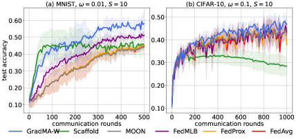
Figure 1: Test accuracy curves selected of GradMA-W as well as baselines over MNIST and CIFAR-10.

Impacts of stragglers. We explore the impacts of different $S$ on MNIST, CIFAR-100 and Tiny-Imagenet. A higher $S$ means more active workers upload updates per communication round. From Table 1, we can clearly see that the performance of all approaches improves uniformly with increasing $S$ on CIFAR-100 and Tiny-Imagenet, where GradMA consistently dominates other baselines in terms of test accuracy. Meanwhile, Fig. 3 shows that the learning efficiency of GradMA consistently outperforms other baselines (see Appendix .2 for more results). However, for MNIST, the test accuracy for most of the approaches does not intuitively improve with increasing $S$. We conjecture that for simple classification tasks and models, the more active workers participating in training, the more prone the centralized model is to overfitting.

Figure 2: Test accuracy curves selected of GradMA-S as well as baselines over CIFAR-100 and Tiny-Imagenet.

Comments on GradMA-W and GradMA-S. We now discuss the empirical performances of GradMA-W and GradMA-S and observe that GradMA-S beats GradMA-W by a significant margin in different FL scenarios, and even slightly outperforms GradMA in a few cases (see Table 1 and Table 2). To put it differently, GradMA leads GradMA-S in most FL scenarios, suggesting that the combination of Worker_Update$()$ and Server_Update$()$ can have a positive effect and thus improve performance. Meanwhile, GradMA-W trumps baselines in most cases, which suggests that Worker_Update$()$ can mitigate the issue of CF and thus augment the centralized model. In addition, we can draw an empirical conclusion that correcting the update direction of the centralized model on the server can greatly boost accuracy compared to correcting that of the local model for each worker. Selected learning curves shown in Fig. 1 and Fig. 4 verify the above statements.

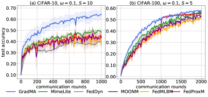
Figure 3: Test accuracy curves selected of GradMA as well as baselines over CIFAR-10 and CIFAR-100.

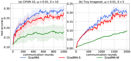
Figure 4: Test accuracy curves selected of GradMA, GradMA-S and GradMA-W over CIFAR-10 and Tiny-Imagenet.

Next, we further explore effects of ($\beta_{1}$, $\beta_{2}$) and $m$ on the performance of GradMA-S on MNIST and CIFAR-10.

Varying control parameters ($\beta_{1}$, $\beta_{2}$). In order to explore effects of ($\beta_{1}$, $\beta_{2}$) in more detail, we set $\beta_{1},\beta_{2}\in\{0.0,0.1,0.3,0.5,0.7,0.9\}$. And we fix $m=100$ and $S=10$. Notice that some similarities exist between GradMA-S and MIFA (MIFAM) when $\beta_{1}=0.0$ and $\beta_{2}=0.0$ ($\beta_{1}=0.0$ and $\beta_{2}>0.0$), i.e., they both memorize the latest updates of stragglers at the server side. From Table 1 and Fig. 5 (refer to Appendix .2 for more results), we can see that GradMA-S with $\beta_{2}=0.0$ considerably beats MIFA and MIFAM regardless of value of $\beta_{1}$. Furthermore, we observe that GradMA-S with $\beta_{2}>0.0$ outperforms GradMA-S with $\beta_{2}=0.0$ in most cases, and the best test accuracy is located in the region of $\beta_{2}>0.0$. This indicates that the accumulated updates of stragglers can provide more effective update information for the centralized model to refine the performance of GradMA-S compared to the latest updates of stragglers.

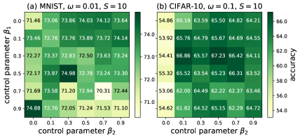
Figure 5: Top test accuracy (%) overview for GradMA-S with varying control parameters ($\beta_{1}$, $\beta_{2}$) on MNIST and CIFAR-10.

Varying memory sizes $m$.

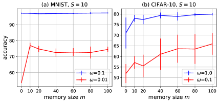
Figure 6: Top test accuracy (%) overview for GradMA-S with varying memory sizes $m$ on MNIST and CIFAR-10.

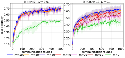
Figure 7: Test accuracy curves selected of GradMA-S with varying memory sizes $m$ on MNIST and CIFAR-10.

In a real-world FL scenario, the memory space on the server side determines the value of the tunable parameter $m$ for GradMA-S. Here, we fix $S=10$ and set $m\in\{0,10,20,40,60,80,100\}$ to carefully look into the performance of GradMA-S with varying $m$. Notably, GradMA-S with $m=0$ is equivalent to FedAvgM. From Fig. 6, FedAvgM performs comparably to GradMA-S with $m>0$ for MNIST under moderate data heterogeneity setting (i.e., $\omega=0.1$). In contrast, the performance of FedAvgM sharply degrades and is seriously worse than that of GradMA-S with $m>0$ under high data heterogeneity setting (i.e., $\omega=0.01$). Meanwhile, for CIFAR-10, GradMA-S with $m>0$ consistently surpasses FedAvgM, even under mild data heterogeneity setting (i.e., $\omega=1.0$). Besides, we can see that the performance of GradMA-S does not intuitively and monotonically improve with increasing $m$. This indicates that the quality of the memory reduction strategy is an essential ingredient affecting the performance of GradMA-S for a given $m$. Therefore, how to tailor a more effective memory reduction strategy is one of our future works. From Fig. 7, the learning curves selected also echo the said statements (see Appendix .2 for more results).

7 Conclusions

In this paper, we propose a novel FL approach GradMA, which corrects the update directions of the server and workers simultaneously. Specifically, on the worker side, GradMA utilizes the gradients of the local model in the previous step and the centralized model, and the parameters difference between the local model in the current round and the centralized model as constraints of QP to adaptively correct the update direction of the local model. On the server side, GradMA takes the memorized accumulated gradients of all workers as constraints of QP to augment the update direction of the centralized model. Meanwhile, we provide the convergence analysis theoretically of GradMA in the smooth non-convex setting. Also, we conduct extensive experiments to verify the superiority of GradMA.

8 Acknowledgments

This work has been supported by the National Natural Science Foundation of China under Grant No.U1911203, and the National Natural Science Foundation of China under Grant No.61977025.

Appendix

.1  Pseudocodes

Algorithm 5 FedAvgM (FedProxM)

1:  Input: learning rates ($\eta_{l}$, $\eta_{g}$), control parameters $\mu$ and $\beta_{1}$, synchronization interval $I$ and the number of workers $N$.

2:  Initial state $\bm{x}_{0}^{(i)}=\bm{x}_{0}\in\mathbb{R}^{d}$, $\forall i\in[N]$ and $\bm{m}_{0}=\bm{0}$.

3:  for $t=0,1,\ldots,T-1$ do

4:     On server:

5:     Server samples a subset $\mathcal{S}_{t}$ with $S$ active workers from $[N]$ and transmits $\bm{x}_{t}$ to $\mathcal{S}_{t}$.

6:     On workers:

7:     for $i\in\mathcal{S}_{t}$ parallel do

8:        Sets $\bm{x}_{t,0}^{(i)}=\bm{x}_{t}$.

9:        for $\tau=0,1,\ldots,I-1$ do

10:           $\bm{x}_{t,\tau+1}^{(i)}=\bm{x}_{t,\tau}^{(i)}-\eta_{l}\nabla f_{i}(\bm{x}_{t,\tau}^{(i)})$. (FedAvgM)

11:           $\bm{x}_{t,\tau+1}^{(i)}=\bm{x}_{t,\tau}^{(i)}-\eta_{l}(\nabla f_{i}(\bm{x}_{t,\tau}^{(i)})+\mu(\bm{x}_{t,\tau}^{(i)}-\bm{x}_{t}))$. (FedProxM)

12:        end for

13:        Sends $\bm{d}_{t+1}^{(i)}=\bm{x}_{t}-\bm{x}_{t,I}^{(i)}$ to server.

14:     end for

15:     On server:

16:     $\bm{d}_{t+1}=\frac{1}{S}\sum_{i\in\mathcal{S}_{t}}\bm{d}_{t+1}^{(i)}$, $\bm{m}_{t+1}=\beta_{1}\bm{m}_{t}+\bm{d}_{t+1}$.

17:     $\bm{x}_{t+1}=\bm{x}_{t}-\eta_{g}\bm{m}_{t+1}$.

18:     Sends $\bm{x}_{t+1}$ to sampled active workers in the next round.

19:  end for

20:  Output: $\bm{x}_{T}$

Algorithm 6 MIFAM (MIFA, i.e., MIFAM with $\beta_{1}=0.0$)

1:  Input: learning rates ($\eta_{l}$, $\eta_{g}$), control parameter $\beta_{1}$, synchronization interval $I$ and the number of workers $N$.

2:  Initial state $\bm{x}_{0}^{(i)}=\bm{x}_{0}\in\mathbb{R}^{d}$, $\bm{g}_{old}^{(i)}=\bm{0}$, $\forall i\in[N]$, $\bm{d}_{0}=\frac{1}{N}\sum_{i=1}^{N}\bm{g}_{old}^{(i)}$ and $\bm{m}_{0}=\bm{0}$.

3:  for $t=0,1,\ldots,T-1$ do

4:     On server:

5:     Server samples a subset $\mathcal{S}_{t}$ with $S$ active workers from $[N]$ and transmits $\bm{x}_{t}$ to $\mathcal{S}_{t}$.

6:     On workers:

7:     for $i\in S_{t}$ parallel do

8:        Sets $\bm{x}_{t,0}^{(i)}=\bm{x}_{t}$.

9:        for $\tau=0,1,\ldots,I-1$ do

10:           $\bm{x}_{t,\tau+1}^{(i)}=\bm{x}_{t,\tau}^{(i)}-\eta_{l}\nabla f_{i}(\bm{x}_{t,\tau}^{(i)})$.

11:        end for

12:        Computes $\bm{g}_{t+1}^{(i)}=\bm{x}_{t}-\bm{x}_{t,I}^{(i)}$.

13:        Sends $\bm{d}_{t+1}^{(i)}=\bm{g}_{t+1}^{(i)}-\bm{g}_{old}^{(i)}$ to Server.

14:        Sets $\bm{g}_{old}^{(i)}=\bm{g}_{t+1}^{(i)}$.

15:     end for

16:     On server:

17:     $\bm{d}_{t+1}=\bm{d}_{t}+\frac{1}{N}\sum_{i\in\mathcal{S}_{t}}\bm{d}_{t+1}^{(i)}$, $\bm{m}_{t+1}=\beta_{1}\bm{m}_{t}+\bm{d}_{t+1}$.

18:     $\bm{x}_{t+1}=\bm{x}_{t}-\eta_{g}\bm{m}_{t+1}$.

19:     Sends $\bm{x}_{t+1}$ to sampled active workers in the next round.

20:  end for

21:  Output: $\bm{x}_{T}$

Algorithm 7 GradMA-W

1:  Input: learning rates ($\eta_{l},\eta_{g}$), the number of all workers $N$, the number of active workers each round $S$ and synchronization interval $I$.

2:  Initial state $\bm{x}_{0}^{(i)}=\bm{x}_{0}\in\mathbbm{R}^{d}$, $\forall i\in[N]$.

3:  for $t=0,1,\ldots,T-1$ do

4:     On server:

5:     Server samples a subset $\mathcal{S}_{t}$ with $S$ active workers and transmits $\bm{x}_{t}$ to $\mathcal{S}_{t}$.

6:     On workers:

7:     for $i\in\mathcal{S}_{t}$ parallel do

8:        $\bm{x}_{t+1}^{(i)}=$ Worker_Update($\bm{x}_{t}^{(i)}$, $\bm{x}_{t}$, $\eta_{l}$, $I$),

9:        sends $\bm{d}_{t+1}^{(i)}=\bm{x}_{t}-\bm{x}_{t+1}^{(i)}$ to server.

10:     end for

11:     On server:

12:     $\bm{d}_{t+1}=\frac{1}{S}\sum_{i\in\mathcal{S}_{t}}\bm{d}_{t+1}^{(i)}$, $\bm{x}_{t+1}=\bm{x}_{t}-\eta_{g}\bm{d}_{t+1}$.

13:     Sends $\bm{x}_{t+1}$ to sampled active workers in the next round.

14:  end for

15:  Output: $\bm{x}_{T}$

Algorithm 8 GradMA-S

1:  Input: learning rates ($\eta_{l},\eta_{g}$), the number of all workers $N$, the number of sampled active workers per communication round $S$, control parameters ($\beta_{1}$, $\beta_{2}$), synchronization interval $I$ and memory size $m$ ($S\leq m\leq\min\{d,N\}$).

2:  Initial state $\bm{x}_{0}^{(i)}=\bm{x}_{0}\in\mathbbm{R}^{d}$, $\forall i\in[N]$, $\tilde{\bm{m}}_{0}=\bm{0}$.

3:  Initial $counter=\{c(i)=0\},\forall i\in[N]$.

4:  Initial memory state $\bm{D}=\{\}$.

5:  $buf=\{\}$, $new\_buf=\{\}$.

6:  for $t=0,1,\ldots,T-1$ do

7:     On server:

8:     Server samples a subset $\mathcal{S}_{t}$ with $S$ active workers and transmits $\bm{x}_{t}$ to $\mathcal{S}_{t}$.

9:     $counter,\bm{D},buf,new\_buf\leftarrow$ mem_red $(m,\mathcal{S}_{t},$ $counter,\bm{D},buf,new\_buf)$.

10:     On workers:

11:     for $i\in\mathcal{S}_{t}$ parallel do

12:        Sets $\bm{x}_{t,0}^{(i)}=\bm{x}_{t}$.

13:        for $\tau=0,1,\ldots,I-1$ do

14:           $\bm{x}_{t,\tau+1}^{(i)}=\bm{x}_{t,\tau}^{(i)}-\eta_{l}\nabla f_{i}(\bm{x}_{t,\tau}^{(i)})$.

15:        end for

16:        Sends $\bm{d}_{t+1}^{(i)}=\bm{x}_{t}-\bm{x}_{t,I}^{(i)}$ to server.

17:     end for

18:     On server:

19:     $\bm{D},\bm{x}_{t+1},\tilde{\bm{m}}_{t+1}=$ Server_Update($[\bm{d}_{t+1}^{(i)},i\in\mathcal{S}_{t}]$, $\tilde{\bm{m}}_{t}$, $\bm{D}$, $\eta_{g}$, $\beta_{1}$, $\beta_{2}$, $buf$, $new\_buf$).

20:     Sends $\bm{x}_{t+1}$ to sampled active workers in the next round.

21:     $new\_buf=\{\}$.

22:  end for

23:  Output: $\bm{x}_{T}$

.2 Complete Empirical Study

.2.1 Experimental Setup

To gauge the effectiveness of Worker_Update$()$ and Server_Update$()$, we perform ablation study of GradMA. For this purpose, we design Alg. 7 (marked as GradMA-W) and Alg. 8 (marked as GradMA-S), as specified in Appendix .1. Meanwhile, we compare other baselines, including FedAvg [26], FedProx [19], MOON [17], FedMLB [13], Scaffold [12], FedDyn [1], MimeLite [11], MIFA [5] and slow-momentum variants of FedAvg, FedProx, MIFA, MOON and FedMLB (i.e., FedAvgM [7], FedProxM, MIFAM, MOONM and FedMLBM), in terms of test accuracy and communication efficiency in different FL scenarios. For fairness, we divide the baselines into three groups based on FedAvg’s improvements on the worker side, server side, or both. Furthermore, on top of GradMA-S, we empirically study the effect of the control parameters ($\beta_{1}$, $\beta_{2}$) and verify the effectiveness of men_red$()$ by setting varying memory sizes $m$.

All our experiments are performed on a centralized network with $100$ workers. And fix synchronization interval $I=5$. To explore the performances of the approaches, we set up multiple different scenarios w.r.t. the number of sampled active workers $S$ per communication round and data heterogeneity. Specifically, we set $S\in\{5,10,50\}$. Furthermore, we use Dirichlet process $Dp(\omega)$ [1, 46] to strictly partition the training set of each dataset across $100$ workers, where the scaling parameter $\omega$ controls the degree of data heterogeneity across workers. Notably, a smaller $\omega$ corresponds to higher data heterogeneity. We set $\omega\in\{0.01,0.1,1.0\}$. A visualization of the data partitions for the four datasets at varying $\omega$ values can be found in Fig. 8. Also, the original testing set (without partitioning) of each dataset is used to evaluate the performance of the trained centralized model. For MNIST, a neural network (NN) with three linear hidden layers is implemented for each worker. We fix the total number of iterations to $2500$, i.e., $T\times I=2500$. For CIFAR-10 (CIFAR-100, Tiny-Imagenet), each worker implements a Lenet-5 [16] (VGG-11 [31], Resnet20 [6]) architecture. We fix the total number of iterations to $5000~{}(10000,10000)$, i.e., $T\times I=5000~{}(10000,10000)$.

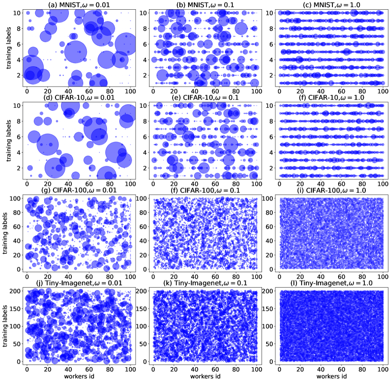
Figure 8: Data heterogeneity among workers is visualized on four datasets (MNIST, CIFAR-10, CIFAR-100 and Tiny-Imagenet), where the $x$-axis represents the workers id, the $y$-axis represents the class labels on the training set, and the size of scattered points represents the number of training samples with available labels for that worker.

We perform careful hyper-parameters tuning of all approaches. We set the local learning rate $\eta_{l}$ for each worker to $\eta_{l}\in\{0.001,0.01,0.1\}$ and the global learning rate $\eta_{g}$ for server to $\eta_{g}\in\{0.1,1.0,10.0\}$. The control parameter $\mu$ for FedProx (FedProxM) and $\alpha$ for FedDyn are fine-tuned within $\{0.001,0.01,0.1\}$. For control parameters ($\beta_{1}$, $\beta_{2}$), we set $\beta_{1},\beta_{2}\in\{0.1,0.5,0.9\}$ unless otherwise specified. Also, we fix memory size $m=100$ unless otherwise specified. For the remaining tunable hyper-parameters of MOON (MOONM) and FedMLB (FedMLBM), we follow the settings of [17] and [13], respectively. For fairness, the popular SGD procedure is employed to perform local update steps for each worker. For all experiments, we fix batch size to $64$ for all datasets. To ensure reliability, we report the average for each experiment over $3$ random seeds.

.2.2 Full Experimental Results

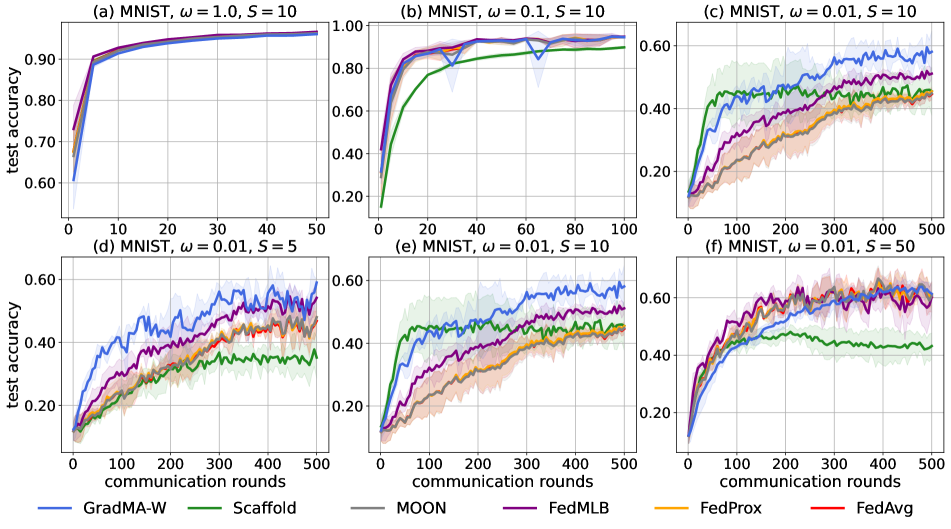
Figure 9: Full test accuracy curves for GradMA-W as well as baselines on MNIST.

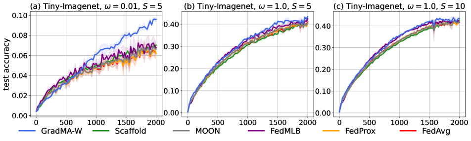
Figure 10: Full test accuracy curves for GradMA-W as well as baselines on Tiny-Imagenet.

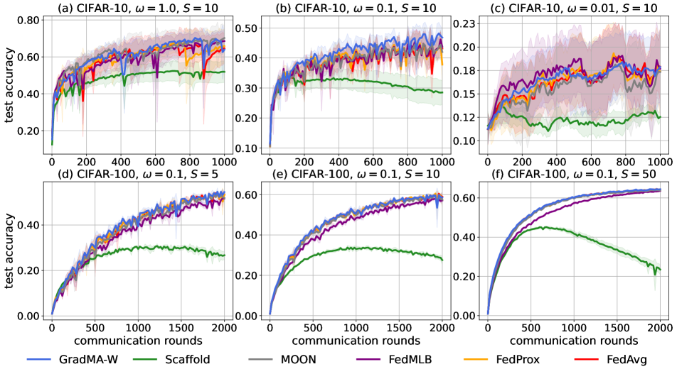
Figure 11: Full test accuracy curves for GradMA-W as well as baselines on CIFAR-10 and CIFAR-100.

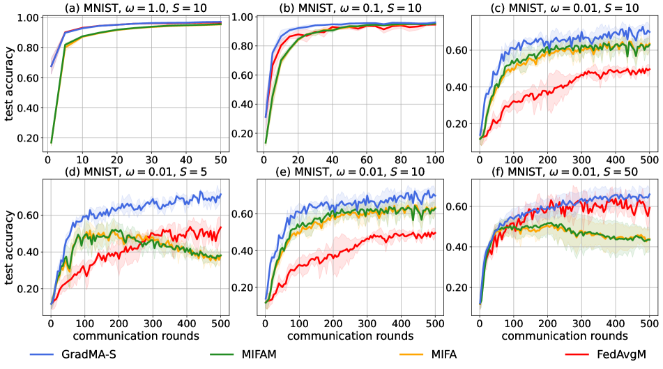
Figure 12: Full test accuracy curves for GradMA-S as well as baselines on MNIST.

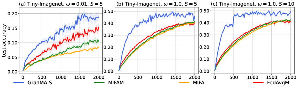
Figure 13: Full test accuracy curves for GradMA-S as well as baselines on Tiny-Imagenet.

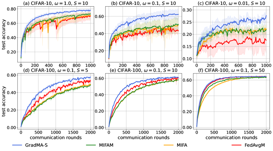
Figure 14: Full test accuracy curves for GradMA-S as well as baselines on CIFAR-10 and CIFAR-100.

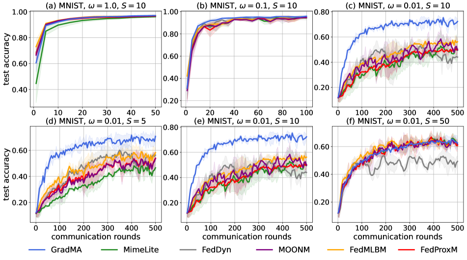
Figure 15: Full test accuracy curves for GradMA as well as baselines on MNIST.

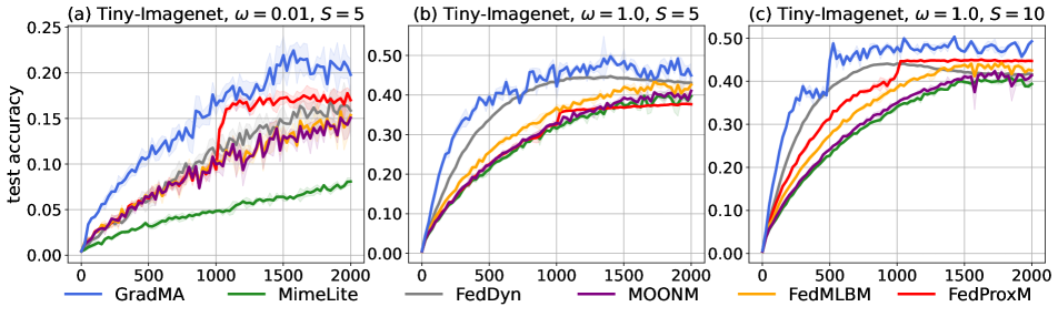
Figure 16: Full test accuracy curves for GradMA as well as baselines on Tiny-Imagenet.

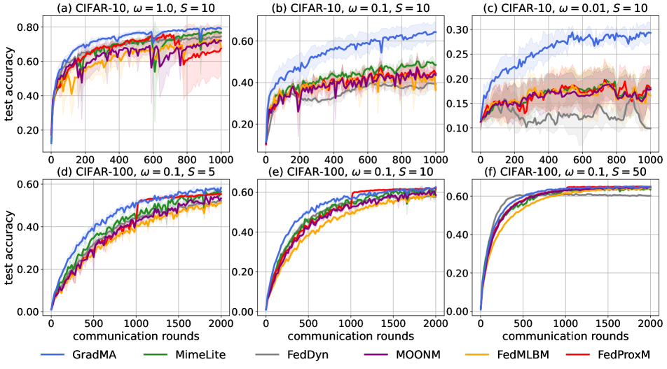
Figure 17: Full test accuracy curves for GradMA as well as baselines on CIFAR-10 and CIFAR-100.

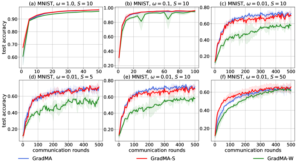
Figure 18: Full test accuracy curves for GradMA, GradMA-S and GradMA-W on MNIST.

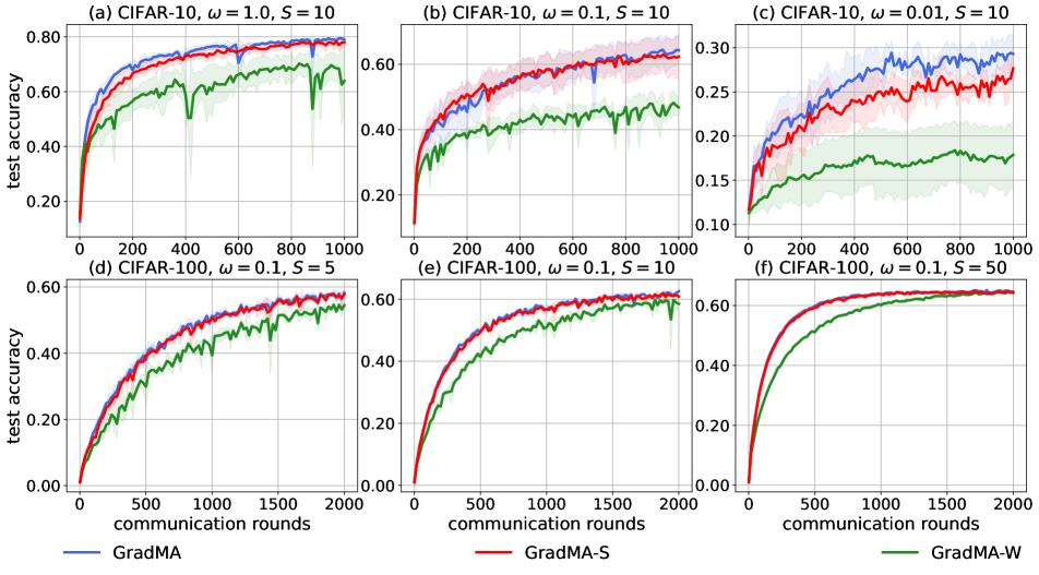
Figure 19: Full test accuracy curves for GradMA, GradMA-S and GradMA-W on CIFAR-10 and CIFAR-100.

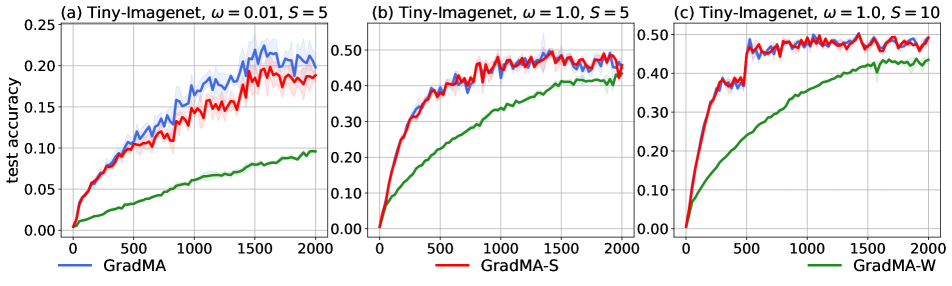
Figure 20: Full test accuracy curves for GradMA, GradMA-S and GradMA-W on Tiny-Imagenet.

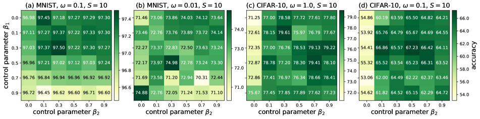
Figure 21: Top test accuracy (%) overview for varying control parameters ($\beta_{1}$,$\beta_{2}$) on MNIST and CIFAR-10.

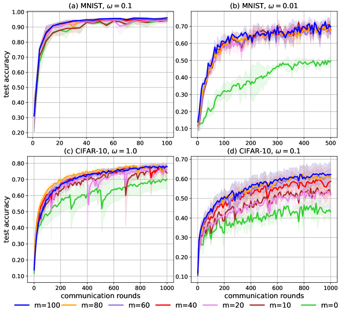
Figure 22: Full test accuracy curves for varying memory sizes $m$ on MNIST and CIFAR-10.

.3  Convergence Proof of GradMA

In this section, we provide the complete theoretical proof for convergence result of GranMA.

We first review the rule for $i$-th ($i\in[N]$) worker to update local model in Alg. 1 and Alg. 2, as follows:

$$\bm{g}_{t,\tau}^{(i)}=\nabla f_{i}(\bm{x}_{t,\tau}^{(i)}),$$ (11)

$$\bm{G}_{t,\tau}^{(i)}=[\nabla f_{i}(\bm{x}_{t,\tau-1}^{(i)}),\nabla f_{i}(\bm{x}_{t}),\bm{x}_{t,\tau}^{(i)}-\bm{x}_{t}],$$ (12)

$$\tilde{\bm{g}}_{t,\tau}^{(i)}={\rm QP}_{l}(\bm{g}_{t,\tau}^{(i)},\bm{G}_{t,\tau}^{(i)}),$$ (13)

$$\bm{x}_{t,\tau+1}^{(i)}=\bm{x}_{t,\tau}^{(i)}-\eta_{l}\tilde{\bm{g}}_{t,\tau}^{(i)},$$ (14)

where $\tau\in[0,\dots,I-1]$ and $\bm{x}_{0,-1}^{(i)}=\bm{x}_{0}^{(i)}=\bm{x}_{0}$, $\bm{x}_{t,-1}^{(i)}=\bm{x}_{t}^{(i)},\bm{x}_{t,0}^{(i)}=\bm{x}_{t}$ ($t>0$).

After receiving update directions sent by active workers, the server updates the centralized model according to the following update rule (see Alg. 1 and Alg. 3):

$$\bm{d}_{t+1}=\frac{1}{S}\sum_{i\in\mathcal{S}_{t}}\bm{d}_{t+1}^{(i)}=\frac{\eta_{l}}{S}\sum_{i\in\mathcal{S}_{t}}\sum_{\tau=0}^{I-1}\tilde{\bm{g}}_{t,\tau}^{(i)},$$ (15)

$$\bm{m}_{t+1}=\beta_{1}\tilde{\bm{m}}_{t}+\bm{d}_{t+1},$$ (16)

$$\tilde{\bm{m}}_{t+1}={\rm QP}_{g}(\bm{m}_{t+1},\bm{D}),$$ (17)

$$\bm{x}_{t+1}=\bm{x}_{t}-\eta_{g}\tilde{\bm{m}}_{t+1},$$ (18)

where $t\in[0,\cdots,T-1]$ and $\tilde{\bm{m}}_{0}=\bm{0}$. Here, we omit the update rule of $\bm{D}$ in that Assumption 5 holds as long as the information contained in $\bm{D}$ is meaningful, without needing to focus on the specific content of $\bm{D}$.

Furthermore, we set $\tilde{\bm{d}}_{t+1}=\bm{d}_{t+1}+\tilde{\bm{m}}_{t+1}-\bm{m}_{t+1}$ yields:

$$\tilde{\bm{m}}_{t+1}=\beta_{1}\tilde{\bm{m}}_{t}+\tilde{\bm{d}}_{t+1},$$ (19)

$$\bm{x}_{t+1}=\bm{x}_{t}-\eta_{g}\tilde{\bm{m}}_{t+1}.$$ (20)

Now, we define an auxiliary sequence such that

$$\bm{u}_{t}=\frac{1}{1-\beta_{1}}\bm{x}_{t}-\frac{\beta_{1}}{1-\beta_{1}}\bm{x}_{t-1},$$ (21)

where $t>0$. If $t=0$ then $\bm{u}_{t}=\bm{x}_{t}$.

Lemma .1

Define the sequence $\{\bm{u}_{t}\}_{t\geq 0}$ as in Eq. (21). According to Alg. 1, we have the following relationship

$$\bm{u}_{t+1}-\bm{u}_{t}=-\frac{\eta_{g}}{1-\beta_{1}}\tilde{\bm{d}}_{t+1}.$$

Proof.  Using mathematical induction on Eq. (21), we get:

case $t=0$,

$$\bm{u}_{t+1}-\bm{u}_{t} =\bm{u}_{1}-\bm{u}_{0}$$

$$=\frac{1}{1-\beta_{1}}\bm{x}_{1}-\frac{\beta_{1}}{1-\beta_{1}}\bm{x}_{0}-\bm{x}_{0}=\frac{1}{1-\beta_{1}}(\bm{x}_{1}-\bm{x}_{0})$$

$$=-\frac{\eta_{g}}{1-\beta_{1}}\tilde{\bm{m}}_{1}=-\frac{\eta_{g}}{1-\beta_{1}}\tilde{\bm{d}}_{1},$$

and case $t>0$,

$$\bm{u}_{t+1}-\bm{u}_{t} =\frac{1}{1-\beta_{1}}\bm{x}_{t+1}-\frac{\beta_{1}}{1-\beta_{1}}\bm{x}_{t}-\frac{1}{1-\beta_{1}}\bm{x}_{t}+\frac{\beta_{1}}{1-\beta_{1}}\bm{x}_{t-1}$$

$$=\frac{1}{1-\beta_{1}}\left((\bm{x}_{t+1}-\bm{x}_{t})-\beta_{1}(\bm{x}_{t}-\bm{x}_{t-1})\right)$$

$$=-\frac{\eta_{g}}{1-\beta_{1}}\left(\bm{m}_{t+1}-\beta_{1}\bm{m}_{t}\right)=-\frac{\eta_{g}}{1-\beta_{1}}\tilde{\bm{d}}_{t+1}.$$

Hence, the lemma is proved.

End Proof.

Lemma .2

Under Assumptions 2-4, then the following relationship generated according to Alg. 1 holds with $\eta_{l}\leq\frac{1}{4\sqrt{10}LI}$: for any $t\in[0,\cdots,T-1]$ and $\tau\in[0,\cdots,I-1]$,

$$\frac{1}{N}\sum_{i\in[N]}\mathbbm{E}\left[\left\|\bm{x}_{t,\tau}^{(i)}-\bm{x}_{t}\right\|^{2}\right]\overset{}{\leq}40I^{2}\eta_{l}^{2}\varepsilon_{l}^{2}+40I^{2}\eta_{l}^{2}\rho^{2}+40I^{2}\eta_{l}^{2}\mathbbm{E}\left[\|\nabla f(\bm{x}_{t})\|^{2}\right],$$

where the expectation $\mathbbm{E}$ is w.r.t the sampled active workers per communication round.

Proof.  For any worker $i\in[N]$ and $\tau\in[1,\cdots,I-1]$, we have:

$$\mathbbm{E} \left[\left\|\bm{x}_{t,\tau}^{(i)}-\bm{x}_{t}\right\|^{2}\right]$$

$$\overset{(a)}{=}\mathbbm{E}\left[\left\|\bm{x}_{t,\tau-1}^{(i)}-\bm{x}_{t}-\eta_{l}\tilde{\bm{g}}_{t,\tau-1}^{(i)}\right\|^{2}\right]$$

$$\overset{}{=}\mathbbm{E}\left[\left\|\bm{x}_{t,\tau-1}^{(i)}-\bm{x}_{t}-\eta_{l}\left(\tilde{\bm{g}}_{t,\tau-1}^{(i)}-\bm{g}_{t,\tau-1}^{(i)}+\nabla f_{i}(\bm{x}_{t,\tau-1}^{(i)})-\nabla f_{i}(\bm{x}_{t})+\nabla f_{i}(\bm{x}_{t})-\nabla f(\bm{x}_{t})+\nabla f(\bm{x}_{t})\right)\right\|^{2}\right]$$

$$\overset{(b)}{\leq}\left(1+\frac{1}{2I-1}\right)\mathbbm{E}\left[\|\bm{x}_{t,\tau-1}^{(i)}-\bm{x}_{t}\|^{2}\right]+8I\eta_{l}^{2}\bigg{[}\mathbbm{E}\left[\|\tilde{\bm{g}}_{t,\tau-1}^{(i)}-\bm{g}_{t,\tau-1}^{(i)}\|^{2}\right]+\mathbbm{E}\left[\|\nabla f_{i}(\bm{x}_{t,\tau-1}^{(i)})-\nabla f_{i}(\bm{x}_{t})\|^{2}\right]$$

$$\quad+\mathbbm{E}\left[\|\nabla f_{i}(\bm{x}_{t})-\nabla f(\bm{x}_{t})\|^{2}\right]+\mathbbm{E}\left[\|\nabla f(\bm{x}_{t})\|^{2}\right]\bigg{]}$$

$$\overset{}{\leq}\left(1+\frac{1}{2I-1}+8I\eta_{l}^{2}L^{2}\right)\mathbbm{E}\left[\|\bm{x}_{t,\tau-1}^{(i)}-\bm{x}_{t}\|^{2}\right]+8I\eta_{l}^{2}\varepsilon_{l}^{2}+8I\eta_{l}^{2}\rho^{2}+8I\eta_{l}^{2}\mathbbm{E}\left[\|\nabla f(\bm{x}_{t})\|^{2}\right]$$

$$\overset{(c)}{\leq}\left(1+\frac{1}{I-1}\right)\mathbbm{E}\left[\|\bm{x}_{t,\tau-1}^{(i)}-\bm{x}_{t}\|^{2}\right]+8I\eta_{l}^{2}\varepsilon_{l}^{2}+8I\eta_{l}^{2}\rho^{2}+8I\eta_{l}^{2}\mathbbm{E}\left[\|\nabla f(\bm{x}_{t})\|^{2}\right],$$ (22)

where ($a$) holds by using the Eq. (14), ($b$) follows from the inequalities $\|\bm{x}\pm\bm{y}\|^{2}\leq(1+\frac{1}{2I-1})\|\bm{x}\|^{2}+2I\|\bm{y}\|^{2},\bm{x},\bm{y}\in\mathbbm{R}^{d}$ and $\left\|\sum_{i=1}^{N}\bm{x}_{i}\right\|^{2}\leq N\sum_{i=1}^{N}\|\bm{x}_{i}\|^{2},\bm{x}_{i}\in\mathbbm{R}^{d}$, and ($c$) holds by using the fact that $\frac{1}{I-1}\geq\frac{1}{2I-1}+8I\eta_{l}^{2}L^{2}$ holds if $\eta_{l}\leq\frac{1}{4\sqrt{10}LI}$.

Then, recursively unrolling inequality (22), we get:

$$\frac{1}{N}\sum_{i\in[N]}\mathbbm{E}\left[\left\|\bm{x}_{t,\tau}^{(i)}-\bm{x}_{t}\right\|^{2}\right] \overset{}{\leq}\sum_{k=0}^{\tau-1}\left(1+\frac{1}{I-1}\right)^{k}\left[8I\eta_{l}^{2}\varepsilon_{l}^{2}+8I\eta_{l}^{2}\rho^{2}+8I\eta_{l}^{2}\mathbbm{E}\left[\|\nabla f(\bm{x}_{t})\|^{2}\right]\right]$$

$$\overset{}{\leq}(I-1)\left[\left(1+\frac{1}{I-1}\right)^{I}-1\right]\left[8I\eta_{l}^{2}\varepsilon_{l}^{2}+8I\eta_{l}^{2}\rho^{2}+8I\eta_{l}^{2}\mathbbm{E}\left[\|\nabla f(\bm{x}_{t})\|^{2}\right]\right]$$

$$\overset{(a)}{\leq}5I\left[8I\eta_{l}^{2}\varepsilon_{l}^{2}+8I\eta_{l}^{2}\rho^{2}+8I\eta_{l}^{2}\mathbbm{E}\left[\|\nabla f(\bm{x}_{t})\|^{2}\right]\right]$$

$$\overset{}{\leq}40I^{2}\eta_{l}^{2}\varepsilon_{l}^{2}+40I^{2}\eta_{l}^{2}\rho^{2}+40I^{2}\eta_{l}^{2}\mathbbm{E}\left[\|\nabla f(\bm{x}_{t})\|^{2}\right],$$

where ($a$) holds by using $\sum_{k=0}^{\tau-1}\left(1+\frac{1}{I-1}\right)^{k}=\frac{1-\left(1+\frac{1}{I-1}\right)^{\tau}}{1-\left(1+\frac{1}{I-1}\right)}=(I-1)\left(\left(1+\frac{1}{I-1}\right)^{\tau}-1\right)\leq(I-1)\left(\left(1+\frac{1}{I-1}\right)^{I}-1\right)\leq 5I$.

So far, we complete the proof.

End Proof.

Lemma .3

Under Assumptions 2-4, then the following relationship generated according to Alg. 1 holds: for any $t\in[0,\cdots,T-1]$,

$$\frac{1}{N}\sum_{i\in[N]}\mathbbm{E}\left[\left\|\sum_{\tau=0}^{I-1}\tilde{\bm{g}}_{t,\tau}^{(i)}\right\|^{2}\right]\overset{}{\leq}4I^{2}(\varepsilon_{l}^{2}+\rho^{2})(1+40I^{2}\eta_{l}^{2}L^{2})+4I^{2}(1+40I^{2}\eta_{l}^{2}L^{2})\mathbbm{E}\left[\left\|\nabla f(\bm{x}_{t})\right\|^{2}\right],$$

where the expectation $\mathbbm{E}$ is w.r.t the sampled active workers per communication round.

Proof.

$$\frac{1}{N}\sum_{i\in[N]} \mathbbm{E}\left[\left\|\sum_{\tau=0}^{I-1}\tilde{\bm{g}}_{t,\tau}^{(i)}\right\|^{2}\right]$$

$$\overset{(a)}{\leq}I\frac{1}{N}\sum_{i\in[N]}\sum_{\tau=0}^{I-1}\mathbbm{E}\left[\left\|\tilde{\bm{g}}_{t,\tau}^{(i)}\right\|^{2}\right]$$

$$\overset{}{\leq}I\frac{1}{N}\sum_{i\in[N]}\sum_{\tau=0}^{I-1}\mathbbm{E}\left[\left\|\tilde{\bm{g}}_{t,\tau}^{(i)}-\bm{g}_{t,\tau}^{(i)}+\nabla f_{i}(\bm{x}_{t,\tau}^{(i)})-\nabla f_{i}(\bm{x}_{t})+\nabla f_{i}(\bm{x}_{t})-\nabla f(\bm{x}_{t})+\nabla f(\bm{x}_{t})\right\|^{2}\right]$$

$$\overset{(b)}{\leq}4I\frac{1}{N}\sum_{i\in[N]}\sum_{\tau=0}^{I-1}\left[\left\|\tilde{\bm{g}}_{t,\tau}^{(i)}-\bm{g}_{t,\tau}^{(i)}\right\|^{2}+\mathbbm{E}\left[\left\|\nabla f_{i}(\bm{x}_{t,\tau}^{(i)})-\nabla f_{i}(\bm{x}_{t})\right\|^{2}\right]+\left\|\nabla f_{i}(\bm{x}_{t})-\nabla f(\bm{x}_{t})\right\|^{2}+\mathbbm{E}\left[\left\|\nabla f(\bm{x}_{t})\right\|^{2}\right]\right]$$

$$\overset{}{\leq}4I\frac{1}{N}\sum_{i\in[N]}\sum_{\tau=0}^{I-1}\left[\varepsilon_{l}^{2}+L^{2}\mathbbm{E}\left[\left\|\bm{x}_{t,\tau}^{(i)}-\bm{x}_{t}\right\|^{2}\right]+\rho^{2}+\mathbbm{E}\left[\left\|\nabla f(\bm{x}_{t})\right\|^{2}\right]\right]$$

$$\overset{}{\leq}4I^{2}\left(\varepsilon_{l}^{2}+\rho^{2}+\mathbbm{E}\left[\left\|\nabla f(\bm{x}_{t})\right\|^{2}\right]\right)+4IL^{2}\frac{1}{N}\sum_{i\in[N]}\sum_{\tau=0}^{I-1}\mathbbm{E}\left[\left\|\bm{x}_{t,\tau}^{(i)}-\bm{x}_{t}\right\|^{2}\right]$$

$$\overset{(c)}{\leq}4I^{2}\left(\varepsilon_{l}^{2}+\rho^{2}+\mathbbm{E}\left[\left\|\nabla f(\bm{x}_{t})\right\|^{2}\right]\right)+4I^{2}L^{2}\left(40I^{2}\eta_{l}^{2}\varepsilon_{l}^{2}+40I^{2}\eta_{l}^{2}\rho^{2}+40I^{2}\eta_{l}^{2}\mathbbm{E}\left[\|\nabla f(\bm{x}_{t})\|^{2}\right]\right)$$

$$\overset{}{\leq}4I^{2}(\varepsilon_{l}^{2}+\rho^{2})(1+40I^{2}\eta_{l}^{2}L^{2})+4I^{2}(1+40I^{2}\eta_{l}^{2}L^{2})\mathbbm{E}\left[\left\|\nabla f(\bm{x}_{t})\right\|^{2}\right]$$

where ($a$) and ($b$) result from the fact that $\left\|\sum_{i=1}^{N}\bm{x}_{i}\right\|^{2}\leq N\sum_{i=1}^{N}\|\bm{x}_{i}\|^{2},\bm{x}_{i}\in\mathbbm{R}^{d}$, and ($c$) uses the statement from Lemma .2.

So far, the lemma is proved.

End Proof.

Lemma .4

Under Assumption 5, then the following relationship generated according to Alg. 1 holds: for any $t\in[0,\cdots,T-1]$,

$$\mathbbm{E}\left[\left\|\tilde{\bm{d}}_{t+1}\right\|^{2}\right]\overset{}{\leq}\frac{2\eta_{l}^{2}}{S^{2}}\mathbbm{E}\left[\left\|\sum_{i\in[N]}\mathbbm{I}\{i\in\mathcal{S}_{t}\}\sum_{\tau=0}^{I-1}\tilde{\bm{g}}_{t,\tau}^{(i)}\right\|^{2}\right]+\frac{2\varepsilon_{g}^{2}}{1-\beta_{2}},$$

where the expectation $\mathbbm{E}$ is w.r.t the sampled active workers per communication round.

Proof.

$$\mathbbm{E}\left[\left\|\tilde{\bm{d}}_{t+1}\right\|^{2}\right] \overset{(a)}{\leq}\mathbbm{E}\left[\left\|\bm{d}_{t+1}+\tilde{\bm{m}}_{t+1}-\bm{m}_{t+1}\right\|^{2}\right]$$

$$\overset{}{\leq}2\mathbbm{E}\left[\left\|\bm{d}_{t+1}\right\|^{2}\right]+2\mathbbm{E}\left[\left\|\tilde{\bm{m}}_{t+1}-\bm{m}_{t+1}\right\|^{2}\right]$$

$$\overset{(b)}{\leq}2\mathbbm{E}\left[\left\|\frac{1}{S}\sum_{i\in\mathcal{S}_{t}}\bm{d}_{t+1}^{(i)}\right\|^{2}\right]+\frac{2\varepsilon_{g}^{2}}{1-\beta_{2}}$$

$$\overset{}{=}\frac{2\eta_{l}^{2}}{S^{2}}\mathbbm{E}\left[\left\|\sum_{i\in[N]}\mathbbm{I}\{i\in\mathcal{S}_{t}\}\sum_{\tau=0}^{I-1}\tilde{\bm{g}}_{t,\tau}^{(i)}\right\|^{2}\right]+\frac{2\varepsilon_{g}^{2}}{1-\beta_{2}},$$

where ($a$) uses the fact that $\tilde{\bm{d}}_{t+1}=\bm{d}_{t+1}+\tilde{\bm{m}}_{t+1}-\bm{m}_{t+1}$, and ($b$) results from the Eq. (15). Hence, the lemma is proved.

End Proof.

Lemma .5

Define the sequence $\{\bm{u}_{t}\}_{t\geq 0}$ as in Eq. (21), the following relationship generated according to Alg. 1 holds: for any $t\in[0,\cdots,T-1]$,

$$\sum_{t=0}^{T-1}\mathbbm{E}\left[\left\|\bm{u}_{t}-\bm{x}_{t}\right\|^{2}\right] \overset{}{\leq}\frac{2\beta_{1}^{2}\eta_{g}^{2}\eta_{l}^{2}}{(1-\beta_{1})^{4}S^{2}}\sum_{t=0}^{T-1}\mathbbm{E}\left[\left\|\sum_{i\in[N]}\mathbbm{I}\{i\in\mathcal{S}_{t}\}\sum_{\tau=0}^{I-1}\tilde{\bm{g}}_{t,\tau}^{(i)}\right\|^{2}\right]+\frac{2\beta_{1}^{2}\eta_{g}^{2}\varepsilon_{g}^{2}T}{(1-\beta_{1})^{4}(1-\beta_{2})},$$

where the expectation $\mathbbm{E}$ is w.r.t the sampled active workers per communication round.

Proof.  Recursively applying Eq. (19) to achieve the update rule for $\tilde{\bm{m}}_{t}$ yields:

$$\tilde{\bm{m}}_{t} \overset{(a)}{=}\sum_{k=1}^{t}\beta_{1}^{t-k}\tilde{\bm{d}}_{k},\forall t\geq 1,$$ (23)

where ($a$) holds by $\tilde{\bm{m}}_{0}=\bm{0}$. Furthermore, building on equations (21) and (23), we get:

$$\bm{u}_{t}-\bm{x}_{t} =\frac{\beta_{1}}{1-\beta_{1}}\left(\bm{x}_{t}-\bm{x}_{t-1}\right)=-\frac{\beta_{1}\eta_{g}}{1-\beta_{1}}\tilde{\bm{m}}_{t}=-\frac{\beta_{1}\eta_{g}}{1-\beta_{1}}\sum_{k=1}^{t}\beta_{1}^{t-k}\tilde{\bm{d}}_{k}.$$ (24)

Now, we define $z_{t}=\sum_{k=1}^{t}\beta_{1}^{t-k}=\frac{1-\beta_{1}^{t}}{1-\beta_{1}},\forall t\geq 1$. Using Eq. (24) we obtain:

$$\mathbbm{E}\left[\left\|\bm{u}_{t}-\bm{x}_{t}\right\|^{2}\right] \overset{}{=}\frac{\beta_{1}^{2}\eta_{g}^{2}}{(1-\beta_{1})^{2}}z_{t}^{2}\mathbbm{E}\left[\left\|\sum_{k=1}^{t}\frac{\beta_{1}^{t-k}}{z_{t}}\tilde{\bm{d}}_{k}\right\|^{2}\right]$$

$$\overset{(a)}{\leq}\frac{\beta_{1}^{2}\eta_{g}^{2}}{(1-\beta_{1})^{2}}z_{t}\sum_{k=1}^{t}\beta_{1}^{t-k}\mathbbm{E}\left[\left\|\tilde{\bm{d}}_{k}\right\|^{2}\right]$$

$$\overset{(b)}{\leq}\frac{\beta_{1}^{2}\eta_{g}^{2}}{(1-\beta_{1})^{3}}\sum_{k=1}^{t}\beta_{1}^{t-k}\mathbbm{E}\left[\left\|\tilde{\bm{d}}_{k}\right\|^{2}\right],$$ (25)

where ($a$) follows from the fact that $\|\sum_{k=1}^{T}\frac{c_{k}}{c}\bm{a}_{k}\|^{2}\leq\sum_{k=1}^{T}\frac{c_{i}}{c}\|\bm{a}_{k}\|^{2}(\bm{a}_{k}\in\mathbbm{R}^{d})$ holds if $c=\sum_{k=1}^{T}c_{k}$, and ($b$) results from $1-\beta^{t}\leq 1$.

Next, summing Eq. (25) over $t\in\{0,\cdots,T-1\}(T\geq 1)$, we have:

$$\sum_{t=0}^{T-1}\mathbbm{E}\left[\left\|\bm{u}_{t}-\bm{x}_{t}\right\|^{2}\right] \overset{(a)}{\leq}\frac{\beta_{1}^{2}\eta_{g}^{2}}{(1-\beta_{1})^{3}}\sum_{t=1}^{T-1}\sum_{k=1}^{t}\beta_{1}^{t-k}\mathbbm{E}\left[\left\|\tilde{\bm{d}}_{k}\right\|^{2}\right]$$

$$\overset{}{=}\frac{\beta_{1}^{2}\eta_{g}^{2}}{(1-\beta_{1})^{3}}\left(\sum_{t=k}^{T-1}\beta_{1}^{t-k}\right)\sum_{k=1}^{T-1}\mathbbm{E}\left[\left\|\tilde{\bm{d}}_{k}\right\|^{2}\right]$$

$$\overset{(b)}{\leq}\frac{\beta_{1}^{2}\eta_{g}^{2}}{(1-\beta_{1})^{4}}\sum_{t=1}^{T-1}\mathbbm{E}\left[\left\|\tilde{\bm{d}}_{t}\right\|^{2}\right]$$

$$\overset{(c)}{\leq}\frac{2\beta_{1}^{2}\eta_{g}^{2}\eta_{l}^{2}}{(1-\beta_{1})^{4}S^{2}}\sum_{t=0}^{T-1}\mathbbm{E}\left[\left\|\sum_{i\in[N]}\mathbbm{I}\{i\in\mathcal{S}_{t}\}\sum_{\tau=0}^{I-1}\tilde{\bm{g}}_{t,\tau}^{(i)}\right\|^{2}\right]+\frac{2\beta_{1}^{2}\eta_{g}^{2}\varepsilon_{g}^{2}T}{(1-\beta_{1})^{4}(1-\beta_{2})},$$ (26)

where ($a$) uses $\bm{u}_{0}=\bm{x}_{0}$, ($b$) holds by using the inequality $\sum_{t=k}^{T-1}\beta_{1}^{t-k}=\frac{1-\beta_{1}^{t}}{1-\beta_{1}}\leq\frac{1}{1-\beta_{1}}$, and ($c$) follows from the statement of Lemma .4.

Hence, the lemma is proved.

End Proof.

Lemma .6

According to Assumptions 1-5 and setting $\eta_{l}\leq\frac{1}{4\sqrt{10}LI}$, $\eta_{g}\eta_{l}\leq\frac{(1-\beta_{1})^{2}S(N-1)}{IL(\beta_{1}S(N-1)+4N(S-1))}$ and $320I^{2}\eta_{l}^{2}L^{2}+\frac{64I\eta_{g}\eta_{l}L(1+40I^{2}\eta_{l}^{2}L^{2})}{(1-\beta_{1})^{2}}\frac{N-S}{S(N-1)}\leq 1$, then the iterates generated by Alg. 1 satisfy: for all $t\in[0,\cdots,T-1]$,

$$\frac{1}{T}\sum_{t=0}^{T-1}\mathbbm{E}\left[\left\|\nabla f(\bm{x}_{t})\right\|^{2}\right] \overset{}{\leq}\frac{8(1-\beta_{1})(f(\bm{x}_{0})-f^{\star})}{I\eta_{g}\eta_{l}T}+8\varepsilon_{l}^{2}+320I^{2}\eta_{l}^{2}L^{2}\varepsilon_{l}^{2}+\frac{64I\eta_{g}\eta_{l}L\varepsilon_{l}^{2}(1+40I^{2}\eta_{l}^{2}L^{2})}{(1-\beta_{1})^{2}}\frac{N-S}{S(N-1)}$$

$$+\frac{20\eta_{g}L\varepsilon_{g}^{2}}{(1-\beta_{1})^{2}(1-\beta_{2})I\eta_{l}}+\frac{8\varepsilon_{g}^{2}}{(1-\beta_{2})I^{2}\eta_{l}^{2}}+320I^{2}\eta_{l}^{2}L^{2}\rho^{2}+\frac{64I\eta_{g}\eta_{l}L\rho^{2}(1+40I^{2}\eta_{l}^{2}L^{2})}{(1-\beta_{1})^{2}}\frac{N-S}{S(N-1)},$$

where the expectation $\mathbbm{E}$ is w.r.t the sampled active workers per communication round.

Proof.  Based on $L$-smooth of $f$ and expectation w.r.t. the sampled active workers per communication round, we have:

$$\mathbbm{E}[f(\bm{u}_{t+1})] \overset{}{\leq}\mathbbm{E}[f(\bm{u}_{t})]+\mathbbm{E}\left[\left\langle\nabla f(\bm{u}_{t}),\bm{u}_{t+1}-\bm{u}_{t}\right\rangle\right]+\frac{L}{2}\mathbbm{E}\left[\left\|\bm{u}_{t+1}-\bm{u}_{t}\right\|^{2}\right]$$

$$\overset{(a)}{=}\mathbbm{E}[f(\bm{u}_{t})]-\frac{\eta_{g}}{1-\beta_{1}}\mathbbm{E}\left[\left\langle\nabla f(\bm{u}_{t}),\tilde{\bm{d}}_{t+1}\right\rangle\right]+\frac{L\eta_{g}^{2}}{2(1-\beta_{1})^{2}}\mathbbm{E}\left[\left\|\tilde{\bm{d}}_{t+1}\right\|^{2}\right]$$

$$\overset{}{=}\mathbbm{E}[f(\bm{u}_{t})]\underbrace{-\frac{\eta_{g}}{1-\beta_{1}}\mathbbm{E}\left[\left\langle\nabla f(\bm{u}_{t})-\nabla f(\bm{x}_{t}),\tilde{\bm{d}}_{t+1}\right\rangle\right]}_{T_{1}}\underbrace{-\frac{\eta_{g}}{1-\beta_{1}}\mathbbm{E}\left[\left\langle\nabla f(\bm{x}_{t}),\tilde{\bm{d}}_{t+1}\right\rangle\right]}_{T_{2}}+\underbrace{\frac{L\eta_{g}^{2}}{2(1-\beta_{1})^{2}}\mathbbm{E}\left[\left\|\tilde{\bm{d}}_{t+1}\right\|^{2}\right]}_{T_{3}},$$ (27)

where ($a$) holds because of the statement of Lemma .1.

Firstly, we note that

$$T_{1} =-\frac{\eta_{g}}{1-\beta_{1}}\mathbbm{E}\left[\left\langle\nabla f(\bm{u}_{t})-\nabla f(\bm{x}_{t}),\tilde{\bm{d}}_{t+1}\right\rangle\right]$$

$$\overset{}{=}-\frac{\eta_{g}}{1-\beta_{1}}\mathbbm{E}\left[\left\langle\nabla f(\bm{u}_{t})-\nabla f(\bm{x}_{t}),\frac{1}{S}\sum_{i\in\mathcal{S}_{t}}\bm{d}_{t+1}^{(i)}\right\rangle\right]-\frac{\eta_{g}}{1-\beta_{1}}\mathbbm{E}\left[\left\langle\nabla f(\bm{u}_{t})-\nabla f(\bm{x}_{t}),\tilde{\bm{m}}_{t+1}-\bm{m}_{t+1}\right\rangle\right]$$

$$\overset{}{=}\underbrace{-\frac{\eta_{g}}{1-\beta_{1}}\mathbbm{E}\left[\left\langle\nabla f(\bm{u}_{t})-\nabla f(\bm{x}_{t}),\frac{1}{N}\sum_{i\in[N]}\bm{d}_{t+1}^{(i)}\right\rangle\right]}_{T_{1,1}}\underbrace{-\frac{\eta_{g}}{1-\beta_{1}}\mathbbm{E}\left[\left\langle\nabla f(\bm{u}_{t})-\nabla f(\bm{x}_{t}),\tilde{\bm{m}}_{t+1}-\bm{m}_{t+1}\right\rangle\right]}_{T_{1,2}}.$$

We proceed by analysis $T_{1,1}$,

$$T_{1,1} \overset{}{=}-\frac{\eta_{g}}{1-\beta_{1}}\mathbbm{E}\left[\left\langle\nabla f(\bm{u}_{t})-\nabla f(\bm{x}_{t}),\frac{1}{N}\sum_{i\in[N]}\bm{d}_{t+1}^{(i)}\right\rangle\right]$$

$$\overset{(a)}{=}-\frac{\eta_{g}}{1-\beta_{1}}\mathbbm{E}\left[\left\langle\nabla f(\bm{u}_{t})-\nabla f(\bm{x}_{t}),\frac{\eta_{l}}{N}\sum_{i\in[N]}\sum_{\tau=0}^{I-1}\tilde{\bm{g}}_{t,\tau}^{(i)}\right\rangle\right]$$

$$\overset{(b)}{\leq}\frac{1-\beta_{1}}{2\beta_{1}L}\mathbbm{E}\left[\|\nabla f(\bm{u}_{t})-\nabla f(\bm{x}_{t})\|^{2}\right]+\frac{\beta_{1}L\eta_{g}^{2}\eta_{l}^{2}}{2(1-\beta_{1})^{3}}\mathbbm{E}\left[\left\|\frac{1}{N}\sum_{i\in[N]}\sum_{\tau=0}^{I-1}\tilde{\bm{g}}_{t,\tau}^{(i)}\right\|^{2}\right]$$

$$\overset{}{\leq}\frac{(1-\beta_{1})L}{2\beta_{1}}\mathbbm{E}\left[\|\bm{u}_{t}-\bm{x}_{t}\|^{2}\right]+\frac{\beta_{1}L\eta_{g}^{2}\eta_{l}^{2}}{2(1-\beta_{1})^{3}N^{2}}\mathbbm{E}\left[\left\|\sum_{i\in[N]}\sum_{\tau=0}^{I-1}\tilde{\bm{g}}_{t,\tau}^{(i)}\right\|^{2}\right],$$

where ($a$) follows by using Eq. (15), and ($b$) holds because of the fact that $\pm\langle\bm{a},\bm{b}\rangle\leq\frac{1}{2}\|\bm{a}\|^{2}+\frac{1}{2}\|\bm{a}\|^{2}~{}(\bm{a},\bm{b}\in\mathbbm{R}^{d})$ where $\bm{a}=-\frac{\sqrt{1-\beta_{1}}}{\sqrt{\beta_{1}L}}(\nabla f(\bm{u}_{t})-\nabla f(\bm{x}_{t}))$ and $\bm{b}=\frac{\sqrt{\beta_{1}L}\eta_{g}\eta_{l}}{(1-\beta_{1})^{3/2}}\frac{1}{N}\sum_{i\in[N]}\sum_{\tau=0}^{I-1}\tilde{\bm{g}}_{t,\tau}^{(i)}$. And we proceed by analysis $T_{1,2}$,

$$T_{1,2} \overset{}{=}-\frac{\eta_{g}}{1-\beta_{1}}\mathbbm{E}\left[\left\langle\nabla f(\bm{u}_{t})-\nabla f(\bm{x}_{t}),\tilde{\bm{m}}_{t+1}-\bm{m}_{t+1}\right\rangle\right]$$

$$\overset{(a)}{\leq}\frac{1-\beta_{1}}{2\beta_{1}L}\mathbbm{E}\left[\left\|\nabla f(\bm{u}_{t})-\nabla f(\bm{x}_{t})\right\|^{2}\right]+\frac{\beta_{1}L\eta_{g}^{2}}{2(1-\beta_{1})^{3}}\mathbbm{E}\left[\left\|\tilde{\bm{m}}_{t+1}-\bm{m}_{t+1}\right\|^{2}\right]$$

$$\overset{}{\leq}\frac{(1-\beta_{1})L}{2\beta_{1}}\mathbbm{E}\left[\left\|\bm{u}_{t}-\bm{x}_{t}\right\|^{2}\right]+\frac{\beta_{1}L\eta_{g}^{2}\varepsilon_{g}^{2}}{2(1-\beta_{1})^{3}(1-\beta_{2})},$$

where ($a$) results from the fact that $\pm\langle\bm{a},\bm{b}\rangle\leq\frac{1}{2}\|\bm{a}\|^{2}+\frac{1}{2}\|\bm{b}\|^{2}~{}(\bm{a},\bm{b}\in\mathbbm{R}^{d})$ where $\bm{a}=-\frac{\sqrt{1-\beta_{1}}}{\sqrt{\beta_{1}L}}(\nabla f(\bm{u}_{t})-\nabla f(\bm{x}_{t}))$ and $\bm{b}=\frac{\sqrt{\beta_{1}L}\eta_{g}}{(1-\beta_{1})^{3/2}}\left(\tilde{\bm{m}}_{t+1}-\bm{m}_{t+1}\right)$.

Secondly, we observe that

$$T_{2} \overset{}{=}-\frac{\eta_{g}}{1-\beta_{1}}\mathbbm{E}\left[\left\langle\nabla f(\bm{x}_{t}),\tilde{\bm{d}}_{t+1}\right\rangle\right]$$

$$\overset{}{=}\underbrace{-\frac{\eta_{g}}{1-\beta_{1}}\mathbbm{E}\left[\left\langle\nabla f(\bm{x}_{t}),\bm{d}_{t+1}\right\rangle\right]}_{T_{2,1}}\underbrace{-\frac{\eta_{g}}{1-\beta_{1}}\mathbbm{E}\left[\left\langle\nabla f(\bm{x}_{t}),\tilde{\bm{m}}_{t+1}-\bm{m}_{t+1}\right\rangle\right]}_{T_{2,2}}.$$

We proceed by analysis $T_{2,1}$,

$$T_{2,1} \overset{}{=}-\frac{\eta_{g}}{1-\beta_{1}}\mathbbm{E}\left[\left\langle\nabla f(\bm{x}_{t}),\bm{d}_{t+1}\right\rangle\right]$$

$$\overset{}{=}-\frac{\eta_{g}}{1-\beta_{1}}\mathbbm{E}\left[\left\langle\nabla f(\bm{x}_{t}),\frac{\eta_{l}}{N}\sum_{i\in[N]}\sum_{\tau=0}^{I-1}\tilde{\bm{g}}_{t,\tau}^{(i)}\right\rangle\right]$$

$$\overset{}{=}-\frac{\eta_{g}}{1-\beta_{1}}\mathbbm{E}\left[\left\langle\nabla f(\bm{x}_{t}),\frac{\eta_{l}}{N}\sum_{i\in[N]}\sum_{\tau=0}^{I-1}\tilde{\bm{g}}_{t,\tau}^{(i)}+\eta_{l}I\nabla f(\bm{x}_{t})-\eta_{l}I\nabla f(\bm{x}_{t})\right\rangle\right]$$

$$\overset{}{=}-\frac{I\eta_{g}\eta_{l}}{1-\beta_{1}}\mathbbm{E}\left[\left\|\nabla f(\bm{x}_{t})\right\|^{2}\right]+\frac{\eta_{g}}{1-\beta_{1}}\mathbbm{E}\left[\left\langle-\sqrt{\eta_{l}I}\nabla f(\bm{x}_{t}),\frac{\sqrt{\eta_{l}}}{\sqrt{I}N}\sum_{i\in[N]}\sum_{\tau=0}^{I-1}\left(\tilde{\bm{g}}_{t,\tau}^{(i)}-\nabla f_{i}(\bm{x}_{t})\right)\right\rangle\right]$$

$$\overset{(a)}{=}-\frac{I\eta_{g}\eta_{l}}{1-\beta_{1}}\mathbbm{E}\left[\left\|\nabla f(\bm{x}_{t})\right\|^{2}\right]+\frac{\eta_{g}}{1-\beta_{1}}\mathbbm{E}\bigg{[}\frac{\eta_{l}I}{2}\|\nabla f(\bm{x}_{t})\|^{2}+\frac{\eta_{l}}{2IN^{2}}\left\|\sum_{i\in[N]}\sum_{\tau=0}^{I-1}\left(\tilde{\bm{g}}_{t,\tau}^{(i)}-\nabla f_{i}(\bm{x}_{t})\right)\right\|^{2}$$

$$\quad\quad\quad\quad\quad\quad\quad\quad\quad\quad\quad\quad\quad\quad\quad\quad\quad\quad\quad\quad\quad\quad\quad\quad\quad\quad\quad\quad\quad\quad\quad-\frac{\eta_{l}}{2IN^{2}}\left\|\sum_{i\in[N]}\sum_{\tau=0}^{I-1}\tilde{\bm{g}}_{t,\tau}^{(i)}\right\|^{2}\bigg{]}$$

$$\overset{}{=}-\frac{I\eta_{g}\eta_{l}}{2(1-\beta_{1})}\mathbbm{E}\left[\left\|\nabla f(\bm{x}_{t})\right\|^{2}\right]+\frac{\eta_{g}\eta_{l}}{2I(1-\beta_{1})N^{2}}\mathbbm{E}\left\|\sum_{i\in[N]}\sum_{\tau=0}^{I-1}\left(\tilde{\bm{g}}_{t,\tau}^{(i)}-\bm{g}_{t,\tau}^{(i)}+\nabla f_{i}(\bm{x}_{t,\tau}^{(i)})-\nabla f_{i}(\bm{x}_{t})\right)\right\|^{2}$$

$$\quad\quad\quad\quad\quad\quad\quad\quad\quad\quad\quad\quad\quad\quad\quad\quad\quad\quad\quad\quad\quad\quad\quad\quad\quad\quad\quad\quad-\frac{\eta_{g}\eta_{l}}{2I(1-\beta_{1})N^{2}}\mathbbm{E}\left\|\sum_{i\in[N]}\sum_{\tau=0}^{I-1}\tilde{\bm{g}}_{t,\tau}^{(i)}\right\|^{2}$$

$$\overset{(b)}{\leq}-\frac{I\eta_{g}\eta_{l}}{2(1-\beta_{1})}\mathbbm{E}\left[\left\|\nabla f(\bm{x}_{t})\right\|^{2}\right]+\frac{\eta_{g}\eta_{l}}{(1-\beta_{1})N}\sum_{i\in[N]}\sum_{\tau=0}^{I-1}\left[\mathbbm{E}\left\|\tilde{\bm{g}}_{t,\tau}^{(i)}-\bm{g}_{t,\tau}^{(i)}\right\|^{2}+\mathbbm{E}\left\|\nabla f_{i}(\bm{x}_{t,\tau}^{(i)})-\nabla f_{i}(\bm{x}_{t})\right\|^{2}\right]$$

$$\quad\quad\quad\quad\quad\quad\quad\quad\quad\quad\quad\quad\quad\quad\quad\quad\quad\quad\quad\quad\quad\quad\quad\quad\quad\quad\quad\quad-\frac{\eta_{g}\eta_{l}}{2I(1-\beta_{1})N^{2}}\mathbbm{E}\left\|\sum_{i\in[N]}\sum_{\tau=0}^{I-1}\tilde{\bm{g}}_{t,\tau}^{(i)}\right\|^{2}$$

$$\overset{}{\leq}-\frac{I\eta_{g}\eta_{l}}{2(1-\beta_{1})}\mathbbm{E}\left[\left\|\nabla f(\bm{x}_{t})\right\|^{2}\right]+\frac{I\eta_{g}\eta_{l}\varepsilon_{l}^{2}}{(1-\beta_{1})}+\frac{\eta_{g}\eta_{l}L^{2}}{(1-\beta_{1})N}\sum_{i\in[N]}\sum_{\tau=0}^{I-1}\mathbbm{E}\left[\left\|\bm{x}_{t,\tau}^{(i)}-\bm{x}_{t}\right\|^{2}\right]$$

$$\quad\quad\quad\quad\quad\quad\quad\quad\quad\quad\quad\quad\quad\quad\quad\quad\quad\quad\quad\quad\quad\quad\quad\quad\quad\quad\quad\quad-\frac{\eta_{g}\eta_{l}}{2I(1-\beta_{1})N^{2}}\mathbbm{E}\left\|\sum_{i\in[N]}\sum_{\tau=0}^{I-1}\tilde{\bm{g}}_{t,\tau}^{(i)}\right\|^{2},$$

where ($a$) follows from the fact that $\pm\langle\bm{a},\bm{b}\rangle=\frac{1}{2}(\|\bm{a}\|^{2}+\|\bm{b}\|^{2}-\|\bm{a}-\bm{b}\|^{2})$, and ($b$) uses the inequality $\left\|\sum_{i=1}^{N}\bm{x}_{i}\right\|^{2}\leq N\sum_{i=1}^{N}\|\bm{x}_{i}\|^{2},\bm{x}_{i}\in\mathbbm{R}^{d}$. And we proceed by analysis $T_{2,2}$,

$$T_{2,2} \overset{}{=}-\frac{\eta_{g}}{1-\beta_{1}}\mathbbm{E}\left[\left\langle\nabla f(\bm{x}_{t}),\tilde{\bm{m}}_{t+1}-\bm{m}_{t+1}\right\rangle\right]$$

$$\overset{(a)}{\leq}\frac{I\eta_{g}\eta_{l}}{4(1-\beta_{1})}\mathbbm{E}\left[\|\nabla f(\bm{x}_{t})\|^{2}\right]+\frac{\eta_{g}}{(1-\beta_{1})I\eta_{l}}\mathbbm{E}\left[\|\tilde{\bm{m}}_{t+1}-\bm{m}_{t+1}\|^{2}\right]$$

$$\overset{}{\leq}\frac{I\eta_{g}\eta_{l}}{4(1-\beta_{1})}\mathbbm{E}\left[\|\nabla f(\bm{x}_{t})\|^{2}\right]+\frac{\eta_{g}\varepsilon_{g}^{2}}{(1-\beta_{1})(1-\beta_{2})I\eta_{l}},$$

where ($a$) using the fact that $\pm\langle\bm{a},\bm{b}\rangle\leq\frac{1}{2}\|\bm{a}\|^{2}+\frac{1}{2}\|\bm{b}\|^{2}~{}(\bm{a},\bm{b}\in\mathbbm{R}^{d})$ where $\bm{a}=-\frac{\sqrt{I\eta_{l}}}{\sqrt{2}}\nabla f(\bm{x}_{t})$ and $\bm{b}=\frac{\sqrt{2}}{\sqrt{I\eta_{l}}}\left(\tilde{\bm{m}}_{t+1}-\bm{m}_{t+1}\right)$.

Next, we utilize the statement of Lemma .4 to derive the following upper bound of $T_{3}$,

$$T_{3} \overset{}{=}\frac{L\eta_{g}^{2}}{2(1-\beta_{1})^{2}}\mathbbm{E}\left[\left\|\tilde{\bm{d}}_{t+1}\right\|^{2}\right]\overset{}{\leq}\frac{L\eta_{g}^{2}\eta_{l}^{2}}{(1-\beta_{1})^{2}S^{2}}\mathbbm{E}\left[\left\|\sum_{i\in[N]}\mathbbm{I}\{i\in\mathcal{S}_{t}\}\sum_{\tau=0}^{I-1}\tilde{\bm{g}}_{t,\tau}^{(i)}\right\|^{2}\right]+\frac{L\eta_{g}^{2}\varepsilon_{g}^{2}}{(1-\beta_{1})^{2}(1-\beta_{2})}.$$

Substituting the upper bounds of $T_{1,1}$, $T_{1,2}$ into $T_{1}$ and $T_{2,1}$, $T_{2,2}$ into $T_{2}$ and $T_{1}$, $T_{2}$, $T_{3}$ into (.3) yields:

$$\mathbbm{E}[f(\bm{u}_{t+1})]$$

$$\leq\mathbbm{E}[f(\bm{u}_{t})]\underbrace{-\frac{\eta_{g}}{1-\beta_{1}}\mathbbm{E}\left[\left\langle\nabla f(\bm{u}_{t})-\nabla f(\bm{x}_{t}),\tilde{\bm{d}}_{t+1}\right\rangle\right]}_{T_{1}}\underbrace{-\frac{\eta_{g}}{1-\beta_{1}}\mathbbm{E}\left[\left\langle\nabla f(\bm{x}_{t}),\tilde{\bm{d}}_{t+1}\right\rangle\right]}_{T_{2}}+\underbrace{\frac{L\eta_{g}^{2}}{2(1-\beta_{1})^{2}}\mathbbm{E}\left[\left\|\tilde{\bm{d}}_{t+1}\right\|^{2}\right]}_{T_{3}}$$

$$\overset{}{\leq}\mathbbm{E}[f(\bm{u}_{t})]-\frac{I\eta_{g}\eta_{l}}{(1-\beta_{1})}\left(\frac{1}{4}-40I^{2}\eta_{l}^{2}L^{2}\right)\mathbbm{E}\left[\left\|\nabla f(\bm{x}_{t})\right\|^{2}\right]+\frac{(1-\beta_{1})L}{\beta_{1}}\mathbbm{E}\left[\|\bm{u}_{t}-\bm{x}_{t}\|^{2}\right]+\frac{\beta_{1}L\eta_{g}^{2}\varepsilon_{g}^{2}}{2(1-\beta_{1})^{3}(1-\beta_{2})}$$

$$+\frac{I\eta_{g}\eta_{l}\varepsilon_{l}^{2}}{(1-\beta_{1})}+\frac{\eta_{g}\varepsilon_{g}^{2}}{(1-\beta_{1})(1-\beta_{2})I\eta_{l}}+\frac{40I^{3}\eta_{g}\eta_{l}^{3}L^{2}\varepsilon_{l}^{2}}{(1-\beta_{1})}+\frac{40I^{3}\eta_{g}\eta_{l}^{3}L^{2}\rho^{2}}{(1-\beta_{1})}+\frac{L\eta_{g}^{2}\varepsilon_{g}^{2}}{(1-\beta_{1})^{2}(1-\beta_{2})}$$

$$-\frac{\eta_{g}\eta_{l}}{2I(1-\beta_{1})N^{2}}\left(1-\frac{\beta_{1}I\eta_{g}\eta_{l}L}{(1-\beta_{1})^{2}}\right)\mathbbm{E}\left[\left\|\sum_{i\in[N]}\sum_{\tau=0}^{I-1}\tilde{\bm{g}}_{t,\tau}^{(i)}\right\|^{2}\right]+\frac{L\eta_{g}^{2}\eta_{l}^{2}}{(1-\beta_{1})^{2}S^{2}}\mathbbm{E}\left[\left\|\sum_{i\in[N]}\mathbbm{I}\{i\in\mathcal{S}_{t}\}\sum_{\tau=0}^{I-1}\tilde{\bm{g}}_{t,\tau}^{(i)}\right\|^{2}\right].$$ (28)

Using the inequality (28), making a simple arrangement and doing the summation operation from $t=0$ to $T-1$, we get:

$$\mathbbm{E}[f(\bm{u}_{T})]-\mathbbm{E}[f(\bm{u}_{0})]$$

$$\overset{}{\leq}-\frac{I\eta_{g}\eta_{l}}{(1-\beta_{1})}\left(\frac{1}{4}-40I^{2}\eta_{l}^{2}L^{2}\right)\sum_{t=0}^{T-1}\mathbbm{E}\left[\left\|\nabla f(\bm{x}_{t})\right\|^{2}\right]+\frac{(1-\beta_{1})L}{\beta_{1}}\sum_{t=0}^{T-1}\mathbbm{E}\left[\|\bm{u}_{t}-\bm{x}_{t}\|^{2}\right]+\frac{\beta_{1}L\eta_{g}^{2}\varepsilon_{g}^{2}T}{2(1-\beta_{1})^{3}(1-\beta_{2})}$$

$$\quad\quad\quad\quad\quad\quad\quad\quad+\frac{I\eta_{g}\eta_{l}\varepsilon_{l}^{2}T}{(1-\beta_{1})}+\frac{\eta_{g}\varepsilon_{g}^{2}T}{(1-\beta_{1})(1-\beta_{2})I\eta_{l}}+\frac{40I^{3}\eta_{g}\eta_{l}^{3}L^{2}\varepsilon_{l}^{2}T}{(1-\beta_{1})}+\frac{40I^{3}\eta_{g}\eta_{l}^{3}L^{2}\rho^{2}T}{(1-\beta_{1})}+\frac{L\eta_{g}^{2}\varepsilon_{g}^{2}T}{(1-\beta_{1})^{2}(1-\beta_{2})}$$

$$\quad-\frac{\eta_{g}\eta_{l}}{2I(1-\beta_{1})N^{2}}\left(1-\frac{\beta_{1}I\eta_{g}\eta_{l}L}{(1-\beta_{1})^{2}}\right)\sum_{t=0}^{T-1}\mathbbm{E}\left[\left\|\sum_{i\in[N]}\sum_{\tau=0}^{I-1}\tilde{\bm{g}}_{t,\tau}^{(i)}\right\|^{2}\right]+\frac{L\eta_{g}^{2}\eta_{l}^{2}}{(1-\beta_{1})^{2}S^{2}}\sum_{t=0}^{T-1}\mathbbm{E}\left[\left\|\sum_{i\in[N]}\mathbbm{I}\{i\in\mathcal{S}_{t}\}\sum_{\tau=0}^{I-1}\tilde{\bm{g}}_{t,\tau}^{(i)}\right\|^{2}\right]$$

$$\overset{(a)}{\leq}-\frac{I\eta_{g}\eta_{l}}{(1-\beta_{1})}\left(\frac{1}{4}-40I^{2}\eta_{l}^{2}L^{2}\right)\sum_{t=0}^{T-1}\mathbbm{E}\left[\left\|\nabla f(\bm{x}_{t})\right\|^{2}\right]+\frac{5\beta_{1}\eta_{g}^{2}L\varepsilon_{g}^{2}T}{2(1-\beta_{1})^{3}(1-\beta_{2})}$$

$$\quad\quad\quad\quad\quad\quad\quad\quad+\frac{I\eta_{g}\eta_{l}\varepsilon_{l}^{2}T}{(1-\beta_{1})}+\frac{\eta_{g}\varepsilon_{g}^{2}T}{(1-\beta_{1})(1-\beta_{2})I\eta_{l}}+\frac{40I^{3}\eta_{g}\eta_{l}^{3}L^{2}\varepsilon_{l}^{2}T}{(1-\beta_{1})}+\frac{40I^{3}\eta_{g}\eta_{l}^{3}L^{2}\rho^{2}T}{(1-\beta_{1})}+\frac{\eta_{g}^{2}L\varepsilon_{g}^{2}T}{(1-\beta_{1})^{2}(1-\beta_{2})}$$

$$\quad\underbrace{-\frac{\eta_{g}\eta_{l}}{2I(1-\beta_{1})N^{2}}\left(1-\frac{\beta_{1}I\eta_{g}\eta_{l}L}{(1-\beta_{1})^{2}}\right)\sum_{t=0}^{T-1}\mathbbm{E}\left[\left\|\sum_{i\in[N]}\sum_{\tau=0}^{I-1}\tilde{\bm{g}}_{t,\tau}^{(i)}\right\|^{2}\right]+\frac{2\eta_{g}^{2}\eta_{l}^{2}L}{(1-\beta_{1})^{3}S^{2}}\sum_{t=0}^{T-1}\mathbbm{E}\left[\left\|\sum_{i\in[N]}\mathbbm{I}\{i\in\mathcal{S}_{t}\}\sum_{\tau=0}^{I-1}\tilde{\bm{g}}_{t,\tau}^{(i)}\right\|^{2}\right]}_{T_{4}},$$ (29)

where ($a$) holds by using the statement of Lemma .5. Next, we derive the upper bound for $T_{4}$. To simplify the proof process, we set $\bm{q}_{t,i}=\sum_{\tau=0}^{I-1}\tilde{\bm{g}}_{t,\tau}^{(i)}$ yields:

$$\mathbbm{E}\left[\left\|\sum_{i\in[N]}\sum_{\tau=0}^{I-1}\tilde{\bm{g}}_{t,\tau}^{(i)}\right\|^{2}\right] \overset{}{=}\mathbbm{E}\left[\left\|\sum_{i\in[N]}\bm{q}_{t,i}\right\|^{2}\right]$$

$$\overset{}{=}\sum_{i\in[N]}\mathbbm{E}\left[\left\|\bm{q}_{t,i}\right\|^{2}\right]+\sum_{i\neq j}\mathbbm{E}\left[\langle\bm{q}_{t,i},\bm{q}_{t,j}\rangle\right]$$

$$\overset{}{=}\sum_{i\in[N]}N\mathbbm{E}\left[\left\|\bm{q}_{t,i}\right\|^{2}\right]-\frac{1}{2}\sum_{i\neq j}\mathbbm{E}\left[\|\bm{q}_{t,i}-\bm{q}_{t,j}\|^{2}\right],$$ (30)

and

$$\mathbbm{E}\left[\left\|\sum_{i\in[N]}\mathbbm{I}\{i\in\mathcal{S}_{t}\}\sum_{\tau=0}^{I-1}\tilde{\bm{g}}_{t,\tau}^{(i)}\right\|^{2}\right] \overset{}{=}\mathbbm{E}\left[\left\|\sum_{i\in[N]}\mathbbm{P}\{i\in\mathcal{S}_{t}\}\bm{q}_{t,i}\right\|^{2}\right]$$

$$\overset{}{=}\sum_{i\in[N]}\mathbbm{P}\{i\in\mathcal{S}_{t}\}\mathbbm{E}\left[\left\|\bm{q}_{t,i}\right\|^{2}\right]+\sum_{i\neq j}\mathbbm{P}\{i,j\in\mathcal{S}_{t}\}\mathbbm{E}\left[\langle\bm{q}_{t,i},\bm{q}_{t,j}\rangle\right]$$

$$\overset{}{=}\frac{S}{N}\sum_{i\in[N]}\mathbbm{E}\left[\left\|\bm{q}_{t,i}\right\|^{2}\right]+\frac{S(S-1)}{N(N-1)}\sum_{i\neq j}\mathbbm{E}\left[\langle\bm{q}_{t,i},\bm{q}_{t,j}\rangle\right]$$

$$\overset{}{=}\frac{S^{2}}{N}\sum_{i\in[N]}\mathbbm{E}\left[\left\|\bm{q}_{t,i}\right\|^{2}\right]-\frac{S(S-1)}{2N(N-1)}\sum_{i\neq j}\mathbbm{E}\left[\|\bm{q}_{t,i}-\bm{q}_{t,j}\|^{2}\right],$$ (31)

where $\mathbbm{P}\{i\in\mathcal{S}_{t}\}=\frac{S}{N}$.

Substituting equalities (30) and (31) into $T_{4}$ yields:

$$T_{4} \overset{}{=}-\frac{\eta_{g}\eta_{l}}{2I(1-\beta_{1})N^{2}}\left(1-\frac{\beta_{1}I\eta_{g}\eta_{l}L}{(1-\beta_{1})^{2}}\right)\sum_{t=0}^{T-1}\mathbbm{E}\left[\left\|\sum_{i\in[N]}\sum_{\tau=0}^{I-1}\tilde{\bm{g}}_{t,\tau}^{(i)}\right\|^{2}\right]+\frac{2\eta_{g}^{2}\eta_{l}^{2}L}{(1-\beta_{1})^{3}S^{2}}\sum_{t=0}^{T-1}\mathbbm{E}\left[\left\|\sum_{i\in[N]}\mathbbm{I}\{i\in\mathcal{S}_{t}\}\sum_{\tau=0}^{I-1}\tilde{\bm{g}}_{t,\tau}^{(i)}\right\|^{2}\right]$$

$$\overset{}{=}-\frac{\eta_{g}\eta_{l}}{2I(1-\beta_{1})N^{2}}\left(1-\frac{\beta_{1}I\eta_{g}\eta_{l}L}{(1-\beta_{1})^{2}}\right)\sum_{t=0}^{T-1}\left[\sum_{i\in[N]}N\mathbbm{E}\left[\left\|\bm{q}_{t,i}\right\|^{2}\right]-\frac{1}{2}\sum_{i\neq j}\mathbbm{E}\left[\|\bm{q}_{t,i}-\bm{q}_{t,j}\|^{2}\right]\right]$$

$$\quad\quad\quad\quad\quad\quad\quad\quad\quad\quad\quad\quad\quad\quad\quad+\frac{2\eta_{g}^{2}\eta_{l}^{2}L}{(1-\beta_{1})^{3}S^{2}}\sum_{t=0}^{T-1}\left[\frac{S^{2}}{N}\sum_{i\in[N]}\mathbbm{E}\left[\left\|\bm{q}_{t,i}\right\|^{2}\right]-\frac{S(S-1)}{2N(N-1)}\sum_{i\neq j}\mathbbm{E}\left[\|\bm{q}_{t,i}-\bm{q}_{t,j}\|^{2}\right]\right]$$

$$\overset{}{=}-\frac{\eta_{g}\eta_{l}}{2I(1-\beta_{1})N}\left(1-\frac{\beta_{1}I\eta_{g}\eta_{l}L}{(1-\beta_{1})^{2}}-\frac{4I\eta_{g}\eta_{l}L}{(1-\beta_{1})^{2}}\right)\sum_{t=0}^{T-1}\sum_{i\in[N]}\mathbbm{E}\left[\left\|\bm{q}_{t,i}\right\|^{2}\right]$$

$$\quad\quad\quad\quad\quad\quad\quad\quad\quad\quad\quad\quad+\frac{\eta_{g}\eta_{l}}{4I(1-\beta_{1})N^{2}}\left(1-\frac{\beta_{1}I\eta_{g}\eta_{l}L}{(1-\beta_{1})^{2}}-\frac{4I\eta_{g}\eta_{l}L}{(1-\beta_{1})^{2}}\frac{N(S-1)}{S(N-1)}\right)\sum_{t=0}^{T-1}\sum_{i\neq j}\mathbbm{E}\left[\|\bm{q}_{t,i}-\bm{q}_{t,j}\|^{2}\right]$$

$$\overset{(a)}{=}-\frac{\eta_{g}\eta_{l}}{2I(1-\beta_{1})N}\left(1-\frac{\beta_{1}I\eta_{g}\eta_{l}L}{(1-\beta_{1})^{2}}-\frac{4I\eta_{g}\eta_{l}L}{(1-\beta_{1})^{2}}\right)\sum_{t=0}^{T-1}\sum_{i\in[N]}\mathbbm{E}\left[\left\|\bm{q}_{t,i}\right\|^{2}\right]$$

$$\quad\quad+\frac{\eta_{g}\eta_{l}}{4I(1-\beta_{1})N^{2}}\left(1-\frac{\beta_{1}I\eta_{g}\eta_{l}L}{(1-\beta_{1})^{2}}-\frac{4I\eta_{g}\eta_{l}L}{(1-\beta_{1})^{2}}\frac{N(S-1)}{S(N-1)}\right)\sum_{t=0}^{T-1}\left[2N\sum_{i\in[N]}\mathbbm{E}\left[\|\bm{q}_{t,i}\|^{2}\right]-2\mathbbm{E}\left[\|\sum_{i\in[N]}\bm{q}_{t,i}\|^{2}\right]\right]$$

$$\overset{}{=}\frac{2\eta_{g}^{2}\eta_{l}^{2}L}{N(1-\beta_{1})^{3}}\left(1-\frac{N(S-1)}{S(N-1)}\right)\sum_{t=0}^{T-1}\sum_{i\in[N]}\mathbbm{E}\left[\left\|\bm{q}_{t,i}\right\|^{2}\right]$$

$$\quad\quad\quad\quad\quad\quad\quad\quad\quad\quad\quad\quad\quad\quad-\frac{\eta_{g}\eta_{l}}{2I(1-\beta_{1})N^{2}}\left(1-\frac{\beta_{1}I\eta_{g}\eta_{l}L}{(1-\beta_{1})^{2}}-\frac{4I\eta_{g}\eta_{l}L}{(1-\beta_{1})^{2}}\frac{N(S-1)}{S(N-1)}\right)\sum_{t=0}^{T-1}\mathbbm{E}\left[\|\sum_{i\in[N]}\bm{q}_{t,i}\|^{2}\right]$$

$$\overset{}{=}\frac{2\eta_{g}^{2}\eta_{l}^{2}L}{(1-\beta_{1})^{3}}\frac{N-S}{NS(N-1)}\sum_{t=0}^{T-1}\sum_{i\in[N]}\mathbbm{E}\left[\left\|\bm{q}_{t,i}\right\|^{2}\right]$$

$$\quad\quad\quad\quad\quad\quad\quad\quad\quad\quad\quad\quad\quad\quad-\frac{\eta_{g}\eta_{l}}{2I(1-\beta_{1})N^{2}}\left(1-\frac{\beta_{1}I\eta_{g}\eta_{l}L}{(1-\beta_{1})^{2}}-\frac{4I\eta_{g}\eta_{l}L}{(1-\beta_{1})^{2}}\frac{N(S-1)}{S(N-1)}\right)\sum_{t=0}^{T-1}\mathbbm{E}\left[\|\sum_{i\in[N]}\bm{q}_{t,i}\|^{2}\right]$$

$$\overset{(b)}{\leq}\frac{2\eta_{g}^{2}\eta_{l}^{2}L}{(1-\beta_{1})^{3}}\frac{N-S}{NS(N-1)}\sum_{t=0}^{T-1}\sum_{i\in[N]}\mathbbm{E}\left[\left\|\bm{q}_{t,i}\right\|^{2}\right]$$

$$\overset{(c)}{\leq}\frac{2\eta_{g}^{2}\eta_{l}^{2}L}{(1-\beta_{1})^{3}}\frac{N-S}{S(N-1)}\left[4I^{2}(\varepsilon_{l}^{2}+\rho^{2})(1+40I^{2}\eta_{l}^{2}L^{2})T+4I^{2}(1+40I^{2}\eta_{l}^{2}L^{2})\sum_{t=0}^{T-1}\mathbbm{E}\left[\left\|\nabla f(\bm{x}_{t})\right\|^{2}\right]\right]$$

$$\overset{}{=}\frac{8I^{2}\eta_{g}^{2}\eta_{l}^{2}L(\varepsilon_{l}^{2}+\rho^{2})(1+40I^{2}\eta_{l}^{2}L^{2})T}{(1-\beta_{1})^{3}}\frac{N-S}{S(N-1)}+\frac{8I^{2}\eta_{g}^{2}\eta_{l}^{2}L(1+40I^{2}\eta_{l}^{2}L^{2})}{(1-\beta_{1})^{3}}\frac{N-S}{S(N-1)}\sum_{t=0}^{T-1}\mathbbm{E}\left[\left\|\nabla f(\bm{x}_{t})\right\|^{2}\right],$$

where ($a$) holds by using $\sum_{i\neq j}\mathbbm{E}\left[\|\bm{q}_{t,i}-\bm{q}_{t,j}\|^{2}\right]=2N\sum_{i\in[N]}\mathbbm{E}\left[\|\bm{q}_{t,i}\|^{2}\right]-2\mathbbm{E}\left[\|\sum_{i\in[N]}\bm{q}_{t,i}\|^{2}\right]$, ($b$) results from the fact that $1-\frac{\beta_{1}I\eta_{g}\eta_{l}L}{(1-\beta_{1})^{2}}-\frac{4I\eta_{g}\eta_{l}L}{(1-\beta_{1})^{2}}\frac{N(S-1)}{S(N-1)}\geq 0$ holds if $\eta_{g}\eta_{l}\leq\frac{(1-\beta_{1})^{2}S(N-1)}{IL(\beta_{1}S(N-1)+4N(S-1))}$, and ($c$) follows from the statement of Lemma .3.

Furthermore, substituting the upper bound of $T_{4}$ into (29), we get:

$$\mathbbm{E}[f(\bm{u}_{T})]-\mathbbm{E}[f(\bm{u}_{0})]$$

$$\overset{}{\leq}-\frac{I\eta_{g}\eta_{l}}{(1-\beta_{1})}\left(\frac{1}{4}-40I^{2}\eta_{l}^{2}L^{2}\right)\sum_{t=0}^{T-1}\mathbbm{E}\left[\left\|\nabla f(\bm{x}_{t})\right\|^{2}\right]+\frac{5\beta_{1}\eta_{g}^{2}L\varepsilon_{g}^{2}T}{2(1-\beta_{1})^{3}(1-\beta_{2})}$$

$$\quad\quad\quad\quad\quad\quad\quad\quad+\frac{I\eta_{g}\eta_{l}\varepsilon_{l}^{2}T}{(1-\beta_{1})}+\frac{\eta_{g}\varepsilon_{g}^{2}T}{(1-\beta_{1})(1-\beta_{2})I\eta_{l}}+\frac{40I^{3}\eta_{g}\eta_{l}^{3}L^{2}\varepsilon_{l}^{2}T}{(1-\beta_{1})}+\frac{40I^{3}\eta_{g}\eta_{l}^{3}L^{2}\rho^{2}T}{(1-\beta_{1})}+\frac{\eta_{g}^{2}L\varepsilon_{g}^{2}T}{(1-\beta_{1})^{2}(1-\beta_{2})}$$

$$\quad\underbrace{-\frac{\eta_{g}\eta_{l}}{2I(1-\beta_{1})N^{2}}\left(1-\frac{\beta_{1}I\eta_{g}\eta_{l}L}{(1-\beta_{1})^{2}}\right)\sum_{t=0}^{T-1}\mathbbm{E}\left[\left\|\sum_{i\in[N]}\sum_{\tau=0}^{I-1}\tilde{\bm{g}}_{t,\tau}^{(i)}\right\|^{2}\right]+\frac{2\eta_{g}^{2}\eta_{l}^{2}L}{(1-\beta_{1})^{3}S^{2}}\sum_{t=0}^{T-1}\mathbbm{E}\left[\left\|\sum_{i\in[N]}\mathbbm{I}\{i\in\mathcal{S}_{t}\}\sum_{\tau=0}^{I-1}\tilde{\bm{g}}_{t,\tau}^{(i)}\right\|^{2}\right]}_{T_{4}}$$

$$\overset{}{\leq}-\frac{I\eta_{g}\eta_{l}}{(1-\beta_{1})}\left(\frac{1}{4}-40I^{2}\eta_{l}^{2}L^{2}\right)\sum_{t=0}^{T-1}\mathbbm{E}\left[\left\|\nabla f(\bm{x}_{t})\right\|^{2}\right]+\frac{5\beta_{1}\eta_{g}^{2}L\varepsilon_{g}^{2}T}{2(1-\beta_{1})^{3}(1-\beta_{2})}$$

$$\quad\quad\quad\quad\quad\quad\quad\quad+\frac{I\eta_{g}\eta_{l}\varepsilon_{l}^{2}T}{(1-\beta_{1})}+\frac{\eta_{g}\varepsilon_{g}^{2}T}{(1-\beta_{1})(1-\beta_{2})I\eta_{l}}+\frac{40I^{3}\eta_{g}\eta_{l}^{3}L^{2}\varepsilon_{l}^{2}T}{(1-\beta_{1})}+\frac{40I^{3}\eta_{g}\eta_{l}^{3}L^{2}\rho^{2}T}{(1-\beta_{1})}+\frac{\eta_{g}^{2}L\varepsilon_{g}^{2}T}{(1-\beta_{1})^{2}(1-\beta_{2})}$$

$$\quad+\frac{8I^{2}\eta_{g}^{2}\eta_{l}^{2}L(\varepsilon_{l}^{2}+\rho^{2})(1+40I^{2}\eta_{l}^{2}L^{2})T}{(1-\beta_{1})^{3}}\frac{N-S}{S(N-1)}+\frac{8I^{2}\eta_{g}^{2}\eta_{l}^{2}L(1+40I^{2}\eta_{l}^{2}L^{2})}{(1-\beta_{1})^{3}}\frac{N-S}{S(N-1)}\sum_{t=0}^{T-1}\mathbbm{E}\left[\left\|\nabla f(\bm{x}_{t})\right\|^{2}\right]$$

$$\overset{}{=}-\frac{I\eta_{g}\eta_{l}}{(1-\beta_{1})}\left(\frac{1}{4}-40I^{2}\eta_{l}^{2}L^{2}-\frac{8I\eta_{g}\eta_{l}L(1+40I^{2}\eta_{l}^{2}L^{2})}{(1-\beta_{1})^{2}}\frac{N-S}{S(N-1)}\right)\sum_{t=0}^{T-1}\mathbbm{E}\left[\left\|\nabla f(\bm{x}_{t})\right\|^{2}\right]+\frac{5\beta_{1}\eta_{g}^{2}L\varepsilon_{g}^{2}T}{2(1-\beta_{1})^{3}(1-\beta_{2})}$$

$$\quad\quad\quad\quad\quad\quad\quad\quad+\frac{I\eta_{g}\eta_{l}\varepsilon_{l}^{2}T}{(1-\beta_{1})}+\frac{\eta_{g}\varepsilon_{g}^{2}T}{(1-\beta_{1})(1-\beta_{2})I\eta_{l}}+\frac{40I^{3}\eta_{g}\eta_{l}^{3}L^{2}\varepsilon_{l}^{2}T}{(1-\beta_{1})}+\frac{40I^{3}\eta_{g}\eta_{l}^{3}L^{2}\rho^{2}T}{(1-\beta_{1})}+\frac{\eta_{g}^{2}L\varepsilon_{g}^{2}T}{(1-\beta_{1})^{2}(1-\beta_{2})}$$

$$\quad\quad\quad\quad\quad\quad\quad\quad\quad\quad\quad\quad\quad\quad\quad\quad\quad\quad\quad\quad\quad\quad\quad\quad\quad\quad\quad+\frac{8I^{2}\eta_{g}^{2}\eta_{l}^{2}L(\varepsilon_{l}^{2}+\rho^{2})(1+40I^{2}\eta_{l}^{2}L^{2})T}{(1-\beta_{1})^{3}}\frac{N-S}{S(N-1)}$$

$$\overset{(a)}{\leq}-\frac{I\eta_{g}\eta_{l}}{8(1-\beta_{1})}\sum_{t=0}^{T-1}\mathbbm{E}\left[\left\|\nabla f(\bm{x}_{t})\right\|^{2}\right]+\frac{5\beta_{1}\eta_{g}^{2}L\varepsilon_{g}^{2}T}{2(1-\beta_{1})^{3}(1-\beta_{2})}+\frac{I\eta_{g}\eta_{l}\varepsilon_{l}^{2}T}{(1-\beta_{1})}+\frac{\eta_{g}\varepsilon_{g}^{2}T}{(1-\beta_{1})(1-\beta_{2})I\eta_{l}}+\frac{40I^{3}\eta_{g}\eta_{l}^{3}L^{2}\varepsilon_{l}^{2}T}{(1-\beta_{1})}$$

$$\quad\quad\quad\quad\quad\quad\quad\quad\quad\quad+\frac{40I^{3}\eta_{g}\eta_{l}^{3}L^{2}\rho^{2}T}{(1-\beta_{1})}+\frac{\eta_{g}^{2}L\varepsilon_{g}^{2}T}{(1-\beta_{1})^{2}(1-\beta_{2})}+\frac{8I^{2}\eta_{g}^{2}\eta_{l}^{2}L(\varepsilon_{l}^{2}+\rho^{2})(1+40I^{2}\eta_{l}^{2}L^{2})T}{(1-\beta_{1})^{3}}\frac{N-S}{S(N-1)},$$ (32)

where ($a$) results from the fact that $\frac{1}{4}-40I^{2}\eta_{l}^{2}L^{2}-\frac{8I\eta_{g}\eta_{l}L(1+40I^{2}\eta_{l}^{2}L^{2})}{(1-\beta_{1})^{2}}\frac{N-S}{S(N-1)}\geq\frac{1}{8}$ holds if $320I^{2}\eta_{l}^{2}L^{2}+\frac{64I\eta_{g}\eta_{l}L(1+40I^{2}\eta_{l}^{2}L^{2})}{(1-\beta_{1})^{2}}\frac{N-S}{S(N-1)}\leq 1$. Now, we use the statement of Assumption 1 yields:

$$f^{\star}-\mathbbm{E}[f(\bm{x}_{0})]\overset{}{\leq}\mathbbm{E}[f(\bm{u}_{T})]-\mathbbm{E}[f(\bm{u}_{0})].$$ (33)

This holds as $\bm{u}_{0}=\bm{x}_{0}$. Finally, the proof of the lemma is completed by substituting inequality (33) into inequality (32) and making a simple arrangement.

End Proof.

References

- [1] Durmus Alp Emre Acar, Yue Zhao, Ramon Matas Navarro, Matthew Mattina, Paul N. Whatmough, and Venkatesh Saligrama. Federated learning based on dynamic regularization. In ICLR, 2021.
- [2] Dmitrii Avdiukhin and Shiva Kasiviswanathan. Federated learning under arbitrary communication patterns. In International Conference on Machine Learning, pages 425–435, 2021.
- [3] Yasaman Esfandiari, Sin Yong Tan, Zhanhong Jiang, Aditya Balu, Ethan Herron, Chinmay Hegde, and Soumik Sarkar. Cross-gradient aggregation for decentralized learning from non-iid data. In International Conference on Machine Learning, pages 3036–3046. PMLR, 2021.
- [4] Mehrdad Farajtabar, Navid Azizan, Alex Mott, and Ang Li. Orthogonal gradient descent for continual learning. In International Conference on Artificial Intelligence and Statistics, pages 3762–3773, 2020.
- [5] Xinran Gu, Kaixuan Huang, Jingzhao Zhang, and Longbo Huang. Fast federated learning in the presence of arbitrary device unavailability. Advances in Neural Information Processing Systems, 34:12052–12064, 2021.
- [6] Kaiming He, Xiangyu Zhang, Shaoqing Ren, and Jian Sun. Deep residual learning for image recognition. In Proceedings of the IEEE conference on computer vision and pattern recognition, pages 770–778, 2016.
- [7] Tzu-Ming Harry Hsu, Hang Qi, and Matthew Brown. Measuring the effects of non-identical data distribution for federated visual classification. arXiv preprint arXiv:1909.06335, 2019.
- [8] Wenke Huang, Mang Ye, and Bo Du. Learn from others and be yourself in heterogeneous federated learning. In CVPR, pages 10143–10153, 2022.
- [9] Meirui Jiang, Zirui Wang, and Qi Dou. Harmofl: Harmonizing local and global drifts in federated learning on heterogeneous medical images. In Proceedings of the AAAI Conference on Artificial Intelligence, volume 36, pages 1087–1095, 2022.
- [10] Peter Kairouz, H Brendan McMahan, Brendan Avent, Aurélien Bellet, Mehdi Bennis, Arjun Nitin Bhagoji, Kallista Bonawitz, Zachary Charles, Graham Cormode, Rachel Cummings, et al. Advances and open problems in federated learning. Foundations and Trends® in Machine Learning, 14(1–2):1–210, 2021.
- [11] Sai Praneeth Karimireddy, Martin Jaggi, Satyen Kale, Mehryar Mohri, Sashank J Reddi, Sebastian U Stich, and Ananda Theertha Suresh. Mime: Mimicking centralized stochastic algorithms in federated learning. arXiv preprint arXiv:2008.03606, 2020.
- [12] Sai Praneeth Karimireddy, Satyen Kale, Mehryar Mohri, Sashank Reddi, Sebastian Stich, and Ananda Theertha Suresh. Scaffold: Stochastic controlled averaging for federated learning. In ICML, pages 5132–5143, 2020.
- [13] Jinkyu Kim, Geeho Kim, and Bohyung Han. Multi-level branched regularization for federated learning. In International Conference on Machine Learning, pages 11058–11073, 2022.
- [14] James Kirkpatrick, Razvan Pascanu, Neil Rabinowitz, Joel Veness, Guillaume Desjardins, Andrei A Rusu, Kieran Milan, John Quan, Tiago Ramalho, Agnieszka Grabska-Barwinska, et al. Overcoming catastrophic forgetting in neural networks. Proceedings of the national academy of sciences, 114(13):3521–3526, 2017.
- [15] A Krizhevsky. Learning multiple layers of features from tiny images. Master’s thesis, University of Tront, 2009.
- [16] Yann LeCun, Léon Bottou, Yoshua Bengio, and Patrick Haffner. Gradient-based learning applied to document recognition. Proceedings of the IEEE, 86(11):2278–2324, 1998.
- [17] Qinbin Li, Bingsheng He, and Dawn Song. Model-contrastive federated learning. In Proceedings of the IEEE/CVF Conference on Computer Vision and Pattern Recognition, pages 10713–10722, 2021.
- [18] Tian Li, Anit Kumar Sahu, Ameet Talwalkar, and Virginia Smith. Federated learning: Challenges, methods, and future directions. IEEE Signal Processing Magazine, 37(3):50–60, 2020.
- [19] Tian Li, Anit Kumar Sahu, Manzil Zaheer, Maziar Sanjabi, Ameet Talwalkar, and Virginia Smith. Federated optimization in heterogeneous networks. Proceedings of Machine Learning and Systems, 2:429–450, 2020.
- [20] Xiang Li, Kaixuan Huang, Wenhao Yang, Shusen Wang, and Zhihua Zhang. On the convergence of fedavg on non-iid data. arXiv preprint arXiv:1907.02189, 2019.
- [21] Xilai Li, Yingbo Zhou, Tianfu Wu, Richard Socher, and Caiming Xiong. Learn to grow: A continual structure learning framework for overcoming catastrophic forgetting. In ICML, pages 3925–3934. PMLR, 2019.
- [22] Yijing Li, Xiaofeng Tao, Xuefei Zhang, Junjie Liu, and Jin Xu. Privacy-preserved federated learning for autonomous driving. IEEE Transactions on Intelligent Transportation Systems, 2021.
- [23] Tao Lin, Lingjing Kong, Sebastian U Stich, and Martin Jaggi. Ensemble distillation for robust model fusion in federated learning. NIPS, 33:2351–2363, 2020.
- [24] David Lopez-Paz and Marc’Aurelio Ranzato. Gradient episodic memory for continual learning. NIPS, 30, 2017.
- [25] Michael McCloskey and Neal J Cohen. Catastrophic interference in connectionist networks: The sequential learning problem. In Psychology of learning and motivation, volume 24, pages 109–165. Elsevier, 1989.
- [26] Brendan McMahan, Eider Moore, Daniel Ramage, Seth Hampson, and Blaise Aguera y Arcas. Communication-efficient learning of deep networks from decentralized data. In International Conference on Artificial Intelligence and Statistics, pages 1273–1282, 2017.
- [27] Dinh C Nguyen, Ming Ding, Pubudu N Pathirana, Aruna Seneviratne, Jun Li, and H Vincent Poor. Federated learning for internet of things: A comprehensive survey. IEEE Communications Surveys & Tutorials, 23(3):1622–1658, 2021.
- [28] Sashank Reddi, Zachary Charles, Manzil Zaheer, Zachary Garrett, Keith Rush, Jakub Konečnỳ, Sanjiv Kumar, and H Brendan McMahan. Adaptive federated optimization. arXiv preprint arXiv:2003.00295, 2020.
- [29] Gobinda Saha, Isha Garg, and Kaushik Roy. Gradient projection memory for continual learning. ICLR, 2021.
- [30] Neta Shoham, Tomer Avidor, Aviv Keren, Nadav Israel, Daniel Benditkis, Liron Mor-Yosef, and Itai Zeitak. Overcoming forgetting in federated learning on non-iid data. NIPS, 2019.
- [31] Karen Simonyan and Andrew Zisserman. Very deep convolutional networks for large-scale image recognition. arXiv preprint arXiv:1409.1556, 2014.
- [32] Shipeng Wang, Xiaorong Li, Jian Sun, and Zongben Xu. Training networks in null space of feature covariance for continual learning. In CVPR, pages 184–193, 2021.
- [33] Yujia Wang, Lu Lin, and Jinghui Chen. Communication-efficient adaptive federated learning. arXiv preprint arXiv:2205.02719, 2022.
- [34] Cong Xie, Sanmi Koyejo, and Indranil Gupta. Asynchronous federated optimization. arXiv preprint arXiv:1903.03934, 2019.
- [35] Ran Xin, Usman Khan, and Soummya Kar. A hybrid variance-reduced method for decentralized stochastic non-convex optimization. In ICML, pages 11459–11469, 2021.
- [36] An Xu and Heng Huang. Coordinating momenta for cross-silo federated learning. AAAI, 36:8735–8743, 2022.
- [37] Chencheng Xu, Zhiwei Hong, Minlie Huang, and Tao Jiang. Acceleration of federated learning with alleviated forgetting in local training. ICLR, 2022.
- [38] Jing Xu, Sen Wang, Liwei Wang, and Andrew Chi-Chih Yao. Fedcm: Federated learning with client-level momentum. arXiv preprint arXiv:2106.10874, 2021.
- [39] Haibo Yang, Minghong Fang, and Jia Liu. Achieving linear speedup with partial worker participation in non-iid federated learning. In ICLR, 2021.
- [40] Haibo Yang, Xin Zhang, Prashant Khanduri, and Jia Liu. Anarchic federated learning. In ICML, pages 25331–25363, 2022.
- [41] Wensi Yang, Yuhang Zhang, Kejiang Ye, Li Li, and Cheng-Zhong Xu. Ffd: A federated learning based method for credit card fraud detection. In International conference on big data, pages 18–32, 2019.
- [42] Dezhong Yao, Wanning Pan, Yutong Dai, Yao Wan, Xiaofeng Ding, Hai Jin, Zheng Xu, and Lichao Sun. Local-global knowledge distillation in heterogeneous federated learning with non-iid data. arXiv preprint arXiv:2107.00051, 2021.
- [43] Jaehong Yoon, Wonyong Jeong, Giwoong Lee, Eunho Yang, and Sung Ju Hwang. Federated continual learning with weighted inter-client transfer. In ICML, pages 12073–12086, 2021.
- [44] Jaehong Yoon, Saehoon Kim, Eunho Yang, and Sung Ju Hwang. Scalable and order-robust continual learning with additive parameter decomposition. arXiv preprint arXiv:1902.09432, 2019.
- [45] Lin Zhang, Li Shen, Liang Ding, Dacheng Tao, and Ling-Yu Duan. Fine-tuning global model via data-free knowledge distillation for non-iid federated learning. In CVPR, pages 10174–10183, 2022.
- [46] Zhuangdi Zhu, Junyuan Hong, and Jiayu Zhou. Data-free knowledge distillation for heterogeneous federated learning. In ICML, pages 12878–12889, 2021.