Multi-Layer Attention-Based Explainability via Transformers for Tabular Data

Abstract

We propose a graph-oriented attention-based explainability method for tabular data. Tasks involving tabular data have been solved mostly using traditional tree-based machine learning models which have the challenges of feature selection and engineering. With that in mind, we consider a transformer architecture for tabular data, which is amenable to explainability, and present a novel way to leverage self-attention mechanism to provide explanations by taking into account the attention matrices of all layers as a whole. The matrices are mapped to a graph structure where groups of features correspond to nodes and attention values to arcs. By finding the maximum probability paths in the graph, we identify groups of features providing larger contributions to explain the model’s predictions. To assess the quality of multi-layer attention-based explanations, we compare them with popular attention-, gradient-, and perturbation-based explanability methods.

1 Introduction

Tabular data (TD) is the most prevalent data modality in real world applications. It is widely used in critical daily-life fields such as medicine, transportation, insurance and finance, many times in combination with additional unstructured data modalities like images, videos, and text. Due to its ubiquity and relevance, it is becoming increasingly common to allow automated systems to use this data as input to models trained to propose or even directly make decisions. Nonetheless, the models are often used without a clear understanding of how and why model decisions come about [9, 33]. Given the nature of the application areas, these decisions may have significant impact and consequences in human lives, highlighting an accentuated need for interpretable and explainable machine learning models. Understanding the rationale behind the decision making of intelligent systems remains the most pertinent factor towards building trust in Artificial Intelligence and further enabling its usage [10, 14].

The huge advances of modern deep learning (DL) models have focused mostly on unstructured data sources [12, 24], as have most of the efforts made towards generating better prediction explanations and interpretable models. For TD, traditional machine learning models such as boosting and random forests continue to be de-facto choices [33]. Yet, despite their good performance, models based on tree ensembles are usually not as interpretable as some simpler -but less successful- models like logistic regression or single decision trees [7]. In this sense, improving DL models for TD would allow both single- and multi-modal problems with TD to benefit from more widely explored explainable models. Additionally, DL models leverage gradient descent learning, which is not supported by tree-based models. This type of optimization decreases the need for feature selection and engineering and facilitates joint training of models taking inputs from multiple data sources with mixed modalities [2, 13].

In particular, a set of models that have shown promising results at pushing the boundaries of DL for TD are transformers [2, 13, 17, 30, 31]. Unlike other DL models, transformers have not only obtained great success in diverse tasks, but also possess a built-in capability to provide explanations for its results via attention [34]. Following this lead, we propose multi-layer attention-based explainability via transformers for TD, a novel method that leverages attention mechanism and combines it with graph concepts to enable a better understanding of how groups of tabular features influence the transformer’s decisions. To this end, a transformer model is trained on a classification task using TD as input. In tabular inputs, it is common to have several features that represent similar underlying concepts. As the number of features increases, their collective importance might end up being diluted across the relative importance of a large number of single features, making it hard to pinpoint relevant explanations at a conceptual level. To account for this, instead of assigning importance or relevance to each individual feature, meaningful groups of features are created a priori. A transformer model is trained with these groups as inputs and the most relevant concepts for the classification task are identified by the model at the conceptual or group level. We train transformers on three datasets and generate multi-layer attention-based explanations for their prediction, i.e., we identify groups of features that have the largest impact on the model’s decision. For a transformer with a single head, prior work considers attention only at the last layer, which disregards information of all preceding layers. Our methodology considers all layers. To cope with the assumption of a single head, we use the student-teacher paradigm to train a single-head but multi-layer transformer based on a trained multi-head transformer and apply graph-based explainability on the student. We further compare our explanations with those provided by other widely known explainability methods.

In summary, the contributions of this work are as follows.

1. We investigate explainable models based on transformers for tabular data.

2. We propose a graph-oriented attention-based explainability method via transformers for tabular data.

3. We compare this approach to attention-, gradient-, and perturbation-based explainability methods.

The rest of this paper is organized as follows. In Section 2, the related work is discussed. Section 3 describes the proposed model: the conceptual transformer model for TD in Section 3.1 and the explainability method used to identify relevant concepts in Section 3.2. Section 4 provides the computational study, experimental details, results, and visualizations. Conclusions are given in Section 5.

2 Related work

2.1 Explainability for Deep Learning

The field of explainable Artificial Intelligence (XAI) has received increasing interest over the past decade. Surveys, reviews, and articles such as [9, 10, 18, 25, 33, 36, 37, 39] have synthesized its main motivations, approaches, and challenges.

In a broad sense, XAI algorithms for DL can be organized into three major groups: perturbation-based, gradient-based, and, more recently, attention-based. Within the most famous perturbation-based methods, we find LIME [23], which generates a local approximation for a given model around a specific prediction, and SHAP [22], which measures a feature’s importance as the change in the expected prediction when conditioning on it. These methods are model agnostic, but have often been applied in DL settings. On the other hand, gradient-based algorithms have focused on DL algorithms, as they leverage gradient information to assess the relevance of the model’s inputs to make its decision. The classic gradient-based methods are saliency maps [28], used for explaining the predictions of convolutional neural networks. In saliency maps, the gradients of the predictor function with respect to the input are computed and used to identify parts of the image that contribute the most either to the final decision or to a specific layer in the network. Another example is Grad-CAM [26], in which gradients are used to compute an importance score that allows class-specific neuron activity visualization in images (referred to as activation maps). A more general gradient-based method is layer-wise relevance propagation [3], while other well known methods falling under this category are Deeplift [27] and SmoothGrad [29].

Attention-based explanations gained relevance along with the success of transformer models [34] in a variety of application areas such as natural language processing, computer vision, and speech processing [20]. Transformers possess a built-in XAI method: the attention mechanism, which generates probability distributions over features and further interprets them as feature importances or contributions. Attention has been further combined with other attributes to generate explanations. For instance, in [38], layer-wise relevance propagation is applied to transformers, and [8] builds on that idea by including gradient information into the explanations. Transformers were initially introduced for machine translation, but have been extended and customized for diverse tasks such as object detection [6] and, more recently to multimodal settings [21, 32]. However, these have focused on vision and language tasks.

2.2 Transformers for Tabular Data

Following the success on unstructured data, transformers have also proven to have good performance on TD. One of the first models to leverage transformers for TD is TabNet [2], which adopts transformer blocks to mimic the structure of decision trees and incorporates sequential attention to select which features to focus on at each step. Similarily, SAINT [30] combines self-attention with inter-sample attention to attend both rows and columns in the TD. TabTransformer [17] uses self-attention transformers to map categorical features to conceptual embeddings. Continuous features are not passed through the transformer architecture, but concatenated with its output for further processing. FT-Transformer [13] introduces a feature tokenizer to adapt the transformer architecture to TD. While all of these methods use attentive transformers on TD, none of them consider multiple layers for explainability of attention or incorporate a priori conceptual information to the architecture. Graphs do come into consideration in graph attention networks [35], neural network architectures that operate on graph-structured data. However, to the best of our knowledge, no work has been done on leveraging graphs for attention matrices.

3 Proposed Model

In this section, we introduce multi-layer attention-based explainability leveraging transformers for TD. We propose the following process. First, a multi-head transformer (teacher) is trained. Then, a single-head (student) transformer is trained based on the output predictions of the teacher. Single-head transformers are more amenable to explanations. Finally, explanations are extracted from the student by using attention values from all layers. In the following subsections, we describe how the transformer architecture is adapted to account for the specific structure of TD and incorporate a priori conceptual information. Next, we describe how we map the underlying self-attention mechanism into attention graphs.

3.1 Conceptual Transformer Encoder for TD

The original transformer model was designed for sequence transduction tasks on text data. TD and text have inherently different structures and as such, their feature engineering strategies differ as well. For instance, preprocessing raw text data is usually done by tokenization, whereas for TD, it is common to normalize numerical features and one-hot-encode categorical.

To account for these differences, two main changes are made to the transformer architecture. First, groups of features representing conceptual information are manually defined before training. Hence, for the TD case, instead of having attention matrices where each word’s projection attends every other word’s projection, we have conceptual groups of features that attend other groups of features. Second, given that TD does not provide sequential information, positional encoding is disabled. The adapted transformer architecture is trained for the classification task at hand.

Let $x_{1}\in\mathcal{R}^{k_{1}}$, $x_{2}\in\mathcal{R}^{k_{2}}$, …, $x_{m}\in\mathcal{R}^{k_{m}}$ be the concept groups of features. We project $x_{i}$ into latent space $\mathcal{R}^{d}$ by defining: $\tilde{x_{i}}=D_{i}x_{i}\in\mathcal{R}^{d}$, with $D_{i}\in\mathcal{R}^{d\times k_{i}}$ trainable. Then, $X=[\tilde{x_{1}},...,\tilde{x_{m}}]^{T}\in\mathcal{R}^{m\times d}$. Following [34], we obtain attention coefficients $a_{i,j}$ by defining $V=XW^{V}$, $K=XW^{K}$, $Q=XW^{Q}$, with $W^{V},W^{K},W^{Q}\in\mathcal{R}^{d\times d}$ trainable matrices, and $V,K,Q\in\mathcal{R}^{m\times d}$. We have that $\frac{QK^{T}}{\sqrt{d}}\in\mathcal{R}^{m\times m}$ and $A=[a_{i,j}]=softmax(\frac{QK^{T}}{\sqrt{d}}V)\in\mathcal{R}^{m\times d}$.

The above-mentioned transformer encoder will then have $N\times h$ attention matrices, where $N$ is the number of encoder layers and $h$ is the number of attention heads. While $N$ and $h$ are tunable hyperparameters, for optimal results they are almost always larger than 1. For XAI purposes, as $N$ and $h$ increase, multi-head attention becomes harder to interpret. To leverage the strengths of multi-head attention while simultaneously prioritizing explainability, we use knowledge distillation [16] as a means to learn a simplified, single-head transformer model (referred to as the student transformer) that can generalize in a similar fashion as the original model (the teacher transformer). The student architecture has $h=1$ and $M$ encoder layers, where $M$ typically meets $M>N$. Furthermore, to improve the entropy of the attention matrices, a penalization term is added to the student’s cross entropy loss function, yielding:

$L=-\sum\limits_{i=1}^{n}y_{i}log(\hat{y}_{i})+\lambda\sum\limits_{l=1}^{M}\sum\limits_{j,k=1}^{m}a^{l}_{j,k}log(a^{l}_{j,k})$

where $n$ is the number of training samples, $\lambda$ is the penalization term hyperparameter, $a^{l}_{j,k}$ is the value in the $j^{th}$ row and $k^{th}$ column of attention matrix $A^{l}$ corresponding to the $l^{th}$ encoder layer, and $y_{i}$ and $\hat{y}_{i}$ are the predictions of the multi-head teacher and the predicted value of the student for sample $i$, respectively.

3.2 Multi-Layer Attention-Based Explainability

Multi-layer attention-based explainability for TD (MLA) leverages the conceptual transformer encoder’s attention mechanism described in Section 3.1 and maps the attention matrices across encoder layers into a directed acyclic graph (DAG). In the DAG, the vertices correspond to concept groups of features and the arcs to attention values. We further identify the concept group with the largest contribution to the prediction, that is, the best concept group to explain the output, as the input group corresponding to the path of the maximum probability in the DAG.

For a given conceptual transformer, we have a collection of attention matrices $A^{l}=(a^{l}_{j,k})$ with $l\in\{1,...,M\}$, and $j,k\in\{1,...,m\}$ as described above. We define $D=(V,A)$ a weighted DAG as follows. Let $V=\bigcup_{l=0}^{M}\{v^{l}_{c}\}$ and $(v^{l-1}_{\hat{c}},v^{l}_{\tilde{c}})\in A$ , where arc $(v^{l-1}_{\hat{c}},v^{l}_{\tilde{c}})$ has weight $a^{l}_{\hat{c},\tilde{c}}$, subscripts $\hat{c}$, $\tilde{c}\in\{1,...,m\}$ correspond to concept groups, superscript $l$ corresponds to encoder layers, and $l=0$ is a special case corresponding to the student’s input layer. In Figure 1, we present a visualization of the construction of $D$.

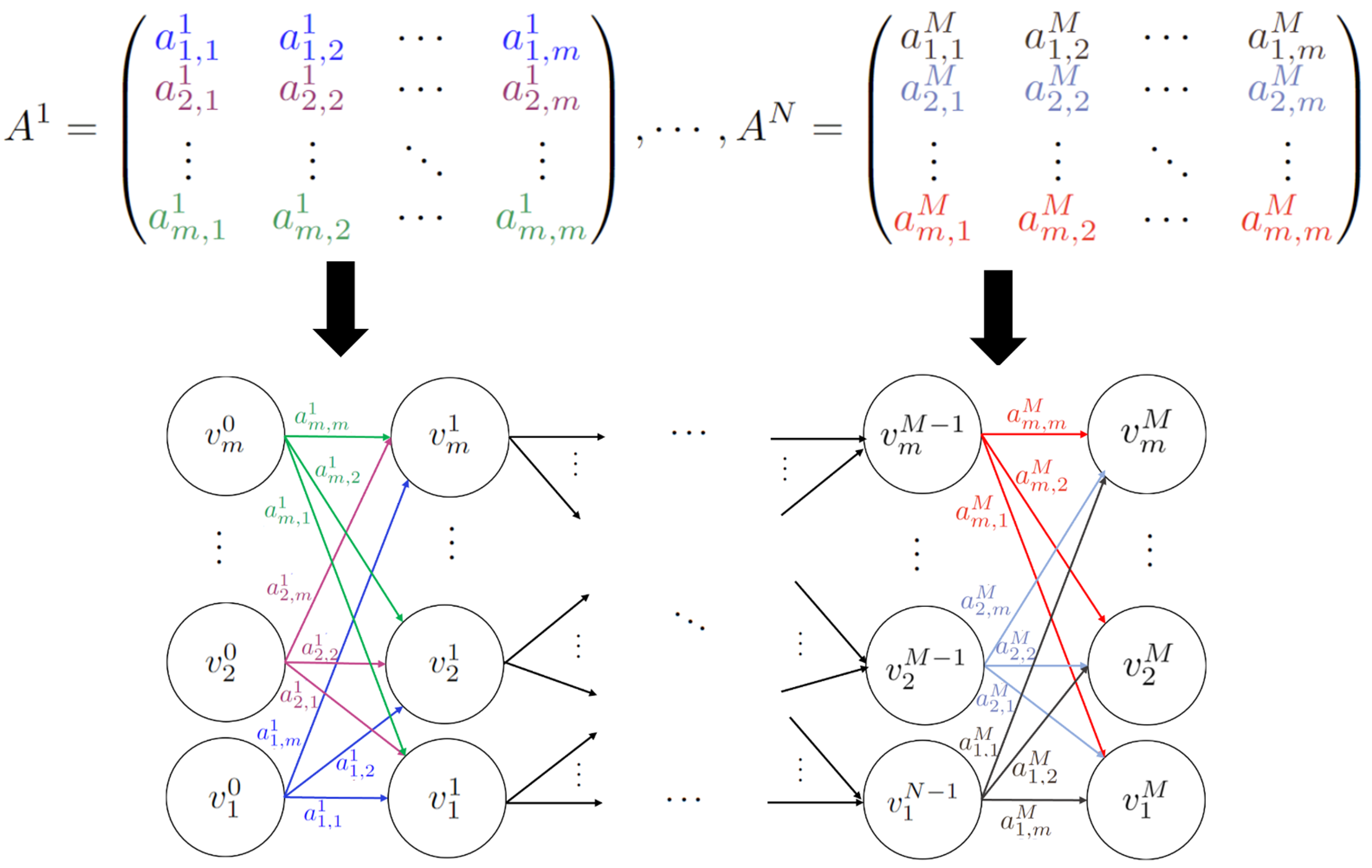
Figure 1: Graph $D=(V,A)$

The maximum probability path $p$ is found using Dijkstra’s algorithm [11], and is of the form $p=\{v^{0}_{i_{0}},v^{1}_{i_{1}},...,v^{M}_{i_{M}}\}$ with arc cost of $-log(a^{l}_{j,k})$ for $a^{l}_{j,k}>0$, yielding path cost $-log\Big{(}\prod_{l=1}^{M}a^{l}_{i_{l-1},i_{l}}\Big{)}$. Since we are particularly interested in the concept group corresponding to the most relevant input for the prediction, we focus on group $c=i_{0}$ corresponding to $v^{0}_{i_{0}}$.

Thus, we provide explanations to the student’s predictions by finding the most relevant concept for the classification task, the best concept group, defined as the concept group $c=i_{0}$ corresponding to the first vertex $v^{0}_{i_{0}}$ of the maximum probability path $p$ in graph $D$. Note that not always does a single concept group provide all the relevant information to make a prediction. To account for this, we rank additional concept groups iteratively. In each iteration we eliminate from the graph the starting point $v^{0}_{i_{0}}$ of the previously found highest probability path and then search for the respective next highest probability path in $D$. In our experiments, we use at most two best concept groups to explain predictions.

4 Computational study

4.1 Datasets

The proposed explainability model is tested on three datasets: UCI Forest CoverType [4], KDD’99 Network Intrusion dataset [15], and a real-world proprietary dataset as described below. These where selected due to their relatively large number of features (with a fair mix of numerical and categorical) and samples, allowing adequate conceptual aggregation.

Forest CoverType Dataset (CT)

In CT, the goal is to predict the most common cover type for each 30m by 30m patch of forest. We use the three most represented classes, resulting in approximately 425,000 training and 53,000 validation samples. The dataset consists of 10 quantitative features and two qualitative features, which were organized into the following five concept groups:

1. Generals: Elevation, aspect, and slope of the patch

2. Distances: Horizontal and vertical distances to hydrology, horizontal distances to roadways and fire points

3. Hillshades: Shades at 9am, noon, and 3pm

4. Wild areas: 4 different wilderness areas

5. Soil types: 40 different types of soil

Network Intrusion Dataset (NI)

In NI, the classification task is to distinguishing between "bad" connections (intrusions or attacks) and "good" connections. Approximately 1,000,000 samples were used for training and almost 75,000 for validation, with each sample consisting of 53 features. The concept groups are defined following [1]:

1. Basic: 20 features regarding individual TCP connections

2. Content: 14 features regarding the connection suggested by domain knowledge

3. Traffic: 9 features computed using a two-second time window

4. Host: 10 features designed to assess attacks which last for more than two seconds

Real-World Dataset (RW)

The proprietary real-world dataset constitutes a binary classification problem. Tens of thousands of samples were used for training and validation. Each sample has approximately 100 features, which were subsequently arranged into 8 concept groups.

4.2 Implementation and hyperparameters

The experiments were implemented in Python and ran using GeForce RTX 2080 Ti GPU and Intel(R) Xeon(R) Silver 4214 CPU @ 2.20GHz for all datasets except RW, for which Tesla V100 GPU and Intel Xeon CPU E5-2697 v4 @2.30Hz were used.

The same hyperparameters were used for all teacher networks: $N=2$, $h=4$, $d=64$ and $128$ neurons in the internal layer. These parameters are standard choices for transformer encoders for TD; on the lower end for $N$ and $h$, and on the higher end for $d$ and neurons. The student’s architecture is identical, but with $M=4$ and $h=1$. For training, we chose a dropout rate of $0.1$ to prevent overfitting while avoiding a large reduction of network’s capacity. Additionally, we used a temperature of $2$, which provided a balance between producing reliable soft targets and avoiding to overly flatten the underlying probability distribution. A constant batch size of $128$ and the adam [19] optimizer were employed. Between six and ten lambdas were tested for each dataset’s training loss. The lambda corresponding to the highest F1 (for CT and NI) and accuracy (for RW) was selected for the final results, yielding $\lambda_{CT}=0.005$, $\lambda_{NI}=0.01$, and $\lambda_{RW}=0.9$. To account for minibatch randomization, each experiment was repeated five times for each CT and NI student and ten times for each RW student, after which variance is already low (see Table 1). In such cases, the best concept group per method was defined as the mode of these experiments. However, the distributions of all repetitions are also presented in the pairwise method comparisons detailed in Section 4.3.

In order to assess the quality of multi-layer attention-based explanations, we first evaluate the performance of the conceptual transformer encoder for TD presented in Section 3.1. The model is compared against two go-to TD methods: LightGBM and XGBoost, with 1,000 base learners each. Other DL and transformer approaches for TD were not considered in this comparison due to their higher computational requirements and similar (if not slightly worse) performance when compared to boosting methods (as reported in [5, 13]). For CT and NI, the aggregated results for five repetitions of each model are shown in Table 1. The conceptual transformer’s performance follows the same patterns previously discussed, comparable but not necessarily better metrics than boosting models.

Table 1: Validation F1

	CT		NI
Models	Mean	Std Dev	Mean	Std Dev
Conceptual Transformer	0.96856	0.00055	0.88715	0.01537
LightGBM	0.96208	0.00063	0.88875	0.00064
XGBoost	0.97268	N/A	0.89226	N/A

Conceptual transformers might not be the top-ranked classifier for all TD cases, but are able to provide explanations for their predictions. As for RW, the conceptual transformer yielded a mean value of $0.88689$ with a standard deviation of $0.00234$. Having validated that its performance is satisfactory, the multi-layer attention-based explanations are extracted as discussed in Section 3.2 and compared to those generated using the most popular method from each XAI group: attention-based, gradient-based and perturbation-based.

Attention-based: Last-layer explainability (LL)

We consider attention mechanism as presented in [34]. More specifically, the last layer’s self-attention head of the student’s encoder. The best concept group to explain a given prediction is defined as that which corresponds to the highest attention value.

Gradient-based: Saliency explainability (SA)

In the same fashion as [28], but in the context of TD, the gradients of the loss function with respect to the input (concept groups) are computed. The best concept group to explain a given prediction is defined as that which yields the largest mean absolute value.

Perturbation-based: Shapley additive explanations (SH)

The SHAP [22] value of each feature is computed. The best concept group is defined as that with the largest mean absolute SHAP value.

4.3 Results

Explanation Distributions

We analyze explanations at an aggregate level in Figure 2, where the distributions of the best concept group per method over the whole validation sets for CT and NI datasets are shown. For each type of explanation, we show the proportion of samples that deemed each concept group as best. In general, we do not distinguish between correctly and wrongly classified samples, unless explicitly stated. For each dataset, the number of incorrectly classified samples is less than $5\%$, which has no impact in the overall distributions (see Appendix B).

(a)

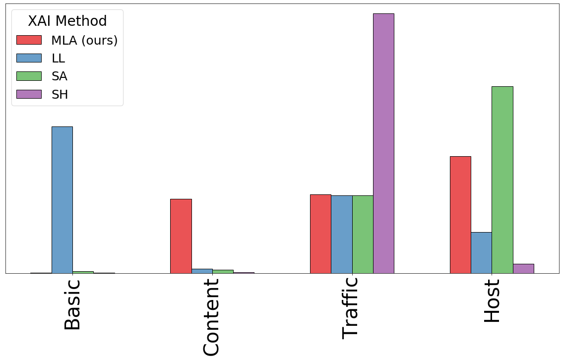
(b)

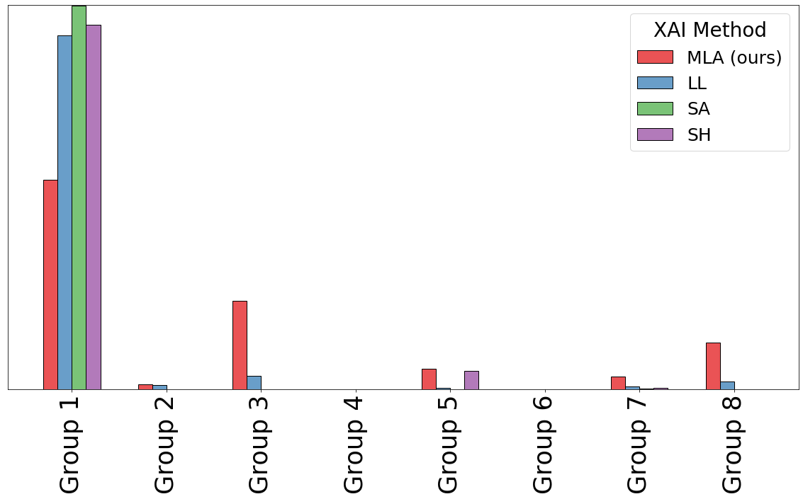
(c)

Figure 2: Best concept group distribution per method

In Figure 2, we observe that SA and SH tend to focus on one or two concept groups to assign predictions, whereas LL and MLA appear to take more groups into account when identifying differences among samples. This behavior is consistent across all datasets. In Figure 3, we zoom in and observe the above-mentioned distributions for CT and NI, but segmented by predicted class.

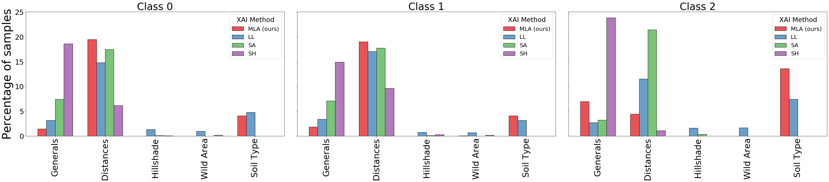
(a) CT

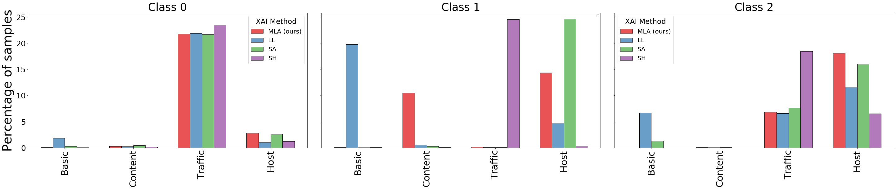
(b) NI

Figure 3: Best group of features per method by class

For CT, a consistent focus on Generals and Distances is observed across all classes. However, LL and MLA seem to also assign large explainability values to Soil Type. A specific focus towards one concept group for a certain class is only observed by SA and SH for the second class. In contrast, the methods show a stronger focus on specific groups for a given class for NI (see Figure 3b). All methods coincide in assigning the largest explainability value to Traffic for class $0$. Interestingly, MLA points at Content and Host as explanations to predict class $1$, whereas LL points at Basic and Host, SA at Host, and SH at Traffic. Additionally, Host and Traffic are consistently referred to as the best concept groups for class $2$ by all groups (with some explanation value assigned to Basic by LL as well).

In summary, we observe large consistency across methods on their best concept group selection for CT, with a particularly strong aligment between LL and MLA. For NI, consistency is notable for classes $0$ and $2$, with LL showing some misaligned samples across all classes.

An Exploratory Data Analysis (EDA) was conducted on CT and NI as a means to validate which features are most relevant for each class. Notably, in Figure 4a, we observe that CT’s features corresponding to concept group Distances do not seem to be particularly distinctive among classes according to their distributions. Perhaps their predictive power is better in conjunction with other groups. In contrast, Figure 4b shows that Soil Type does provide a clear differentiation between classes. All samples from class $2$ have soil types in $\{0,...,9\}$, whereas samples from class $0$ do not have soil types lower than $9$. Even though the EDA clearly shows Soil Type concept group’s relevance for the classification task, only LL and MLA methods capture this information.

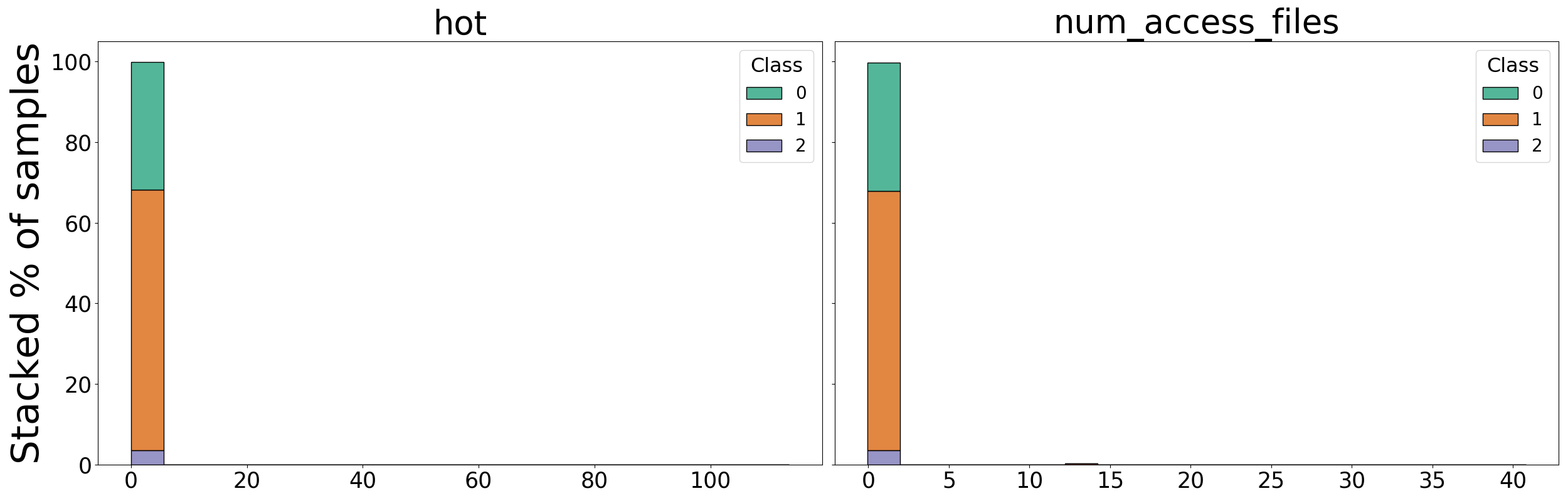
(a)

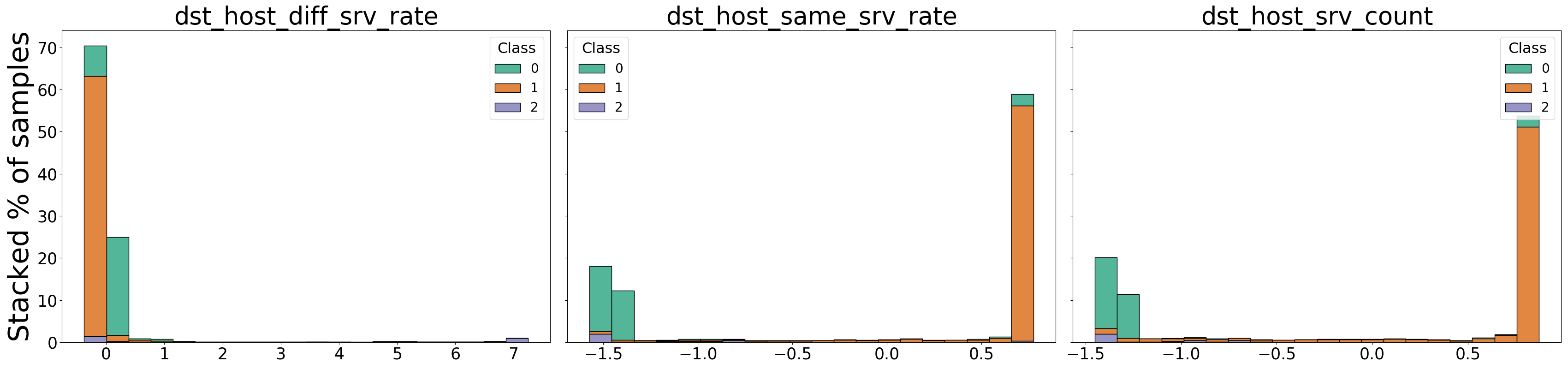
(b)

(a) Density of Content and Host features

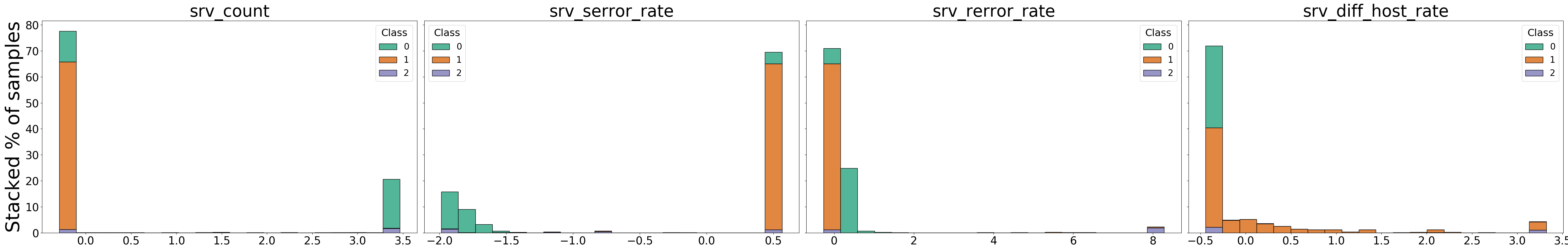
(b) Density of Traffic features

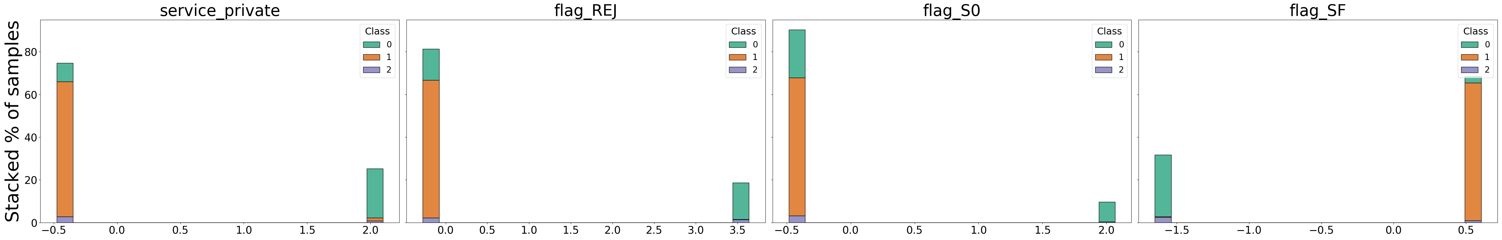
(c) Density of Basic features

Figure 11: NI EDA

In the NI dataset most features are continuous. Hence, only a small subset of them are presented and shown in Figure 11 in the Appendix. Through a similar EDA, we observe that Host and Traffic are indicative of all classes, which is consistent with most of the distributions shown in Figure 3b. However, for several samples of class $1$, LL assigns Basic and MLA assigns Content as the best concept groups, while these correspondences are less clear in the EDA.

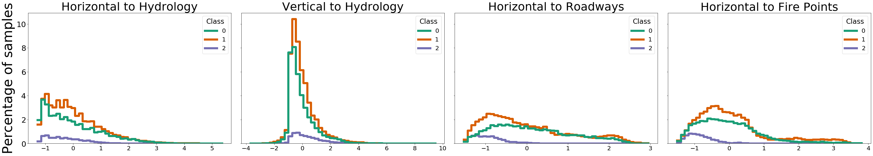
(a) Density of relevant distances features

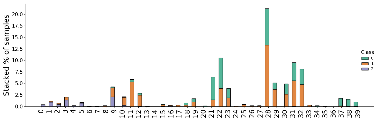
(b) Number of samples per Soil Type

Figure 4: CT EDA

We conclude that LL and MLA are better aligned with the findings of the EDA. For classes $0$ and $1$, both methods show similar correspondences -and disagreements- with it. However, for the least represented class in each dataset (class $2$), MLA’s aligment to the EDA appears better than LL’s, as it focuses on the groups highlighted by the EDA for a larger number of samples.

Explanation Visualizations

To get a visual representation of the explanations for a given sample, each of the compared methods’ explainability values for each concept group are plotted in the heatmaps below. In the 2D heatmaps, for $j,k\in{1,...,m}$, the values for MLA to the the probability of the maximum probability path $p$ between $v^{0}_{j}$ and $v^{M}_{k}$, whereas the values for LL correspond to $a^{M}_{j,k}$. Lighter color tones correspond to lower explainability values. For comparability across methods, values have been scaled to $[0,1]$ and only correctly classified samples were considered.

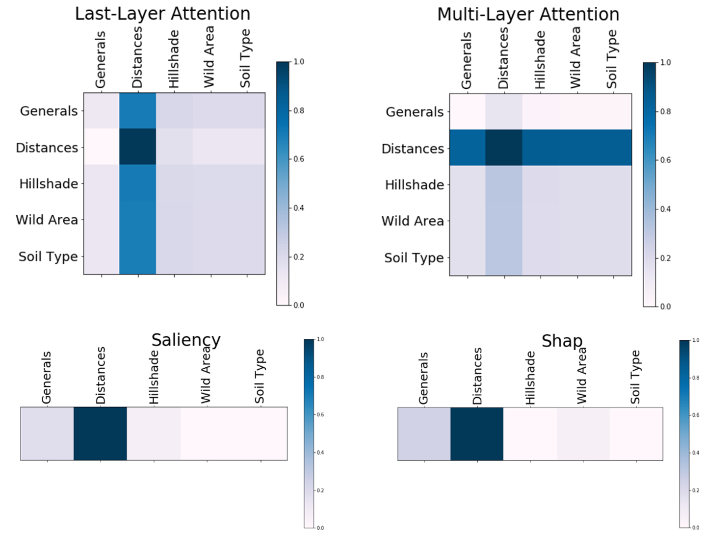
(a)

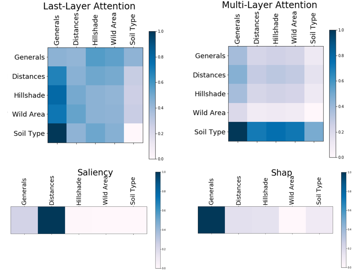
(b)

Figure 5: CT Concept groups explainability coefficients

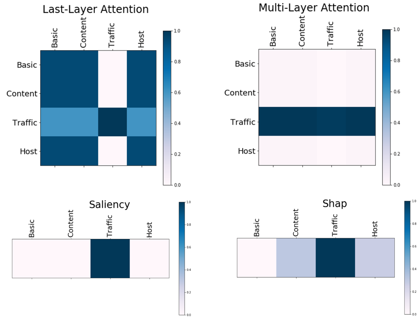
(a)

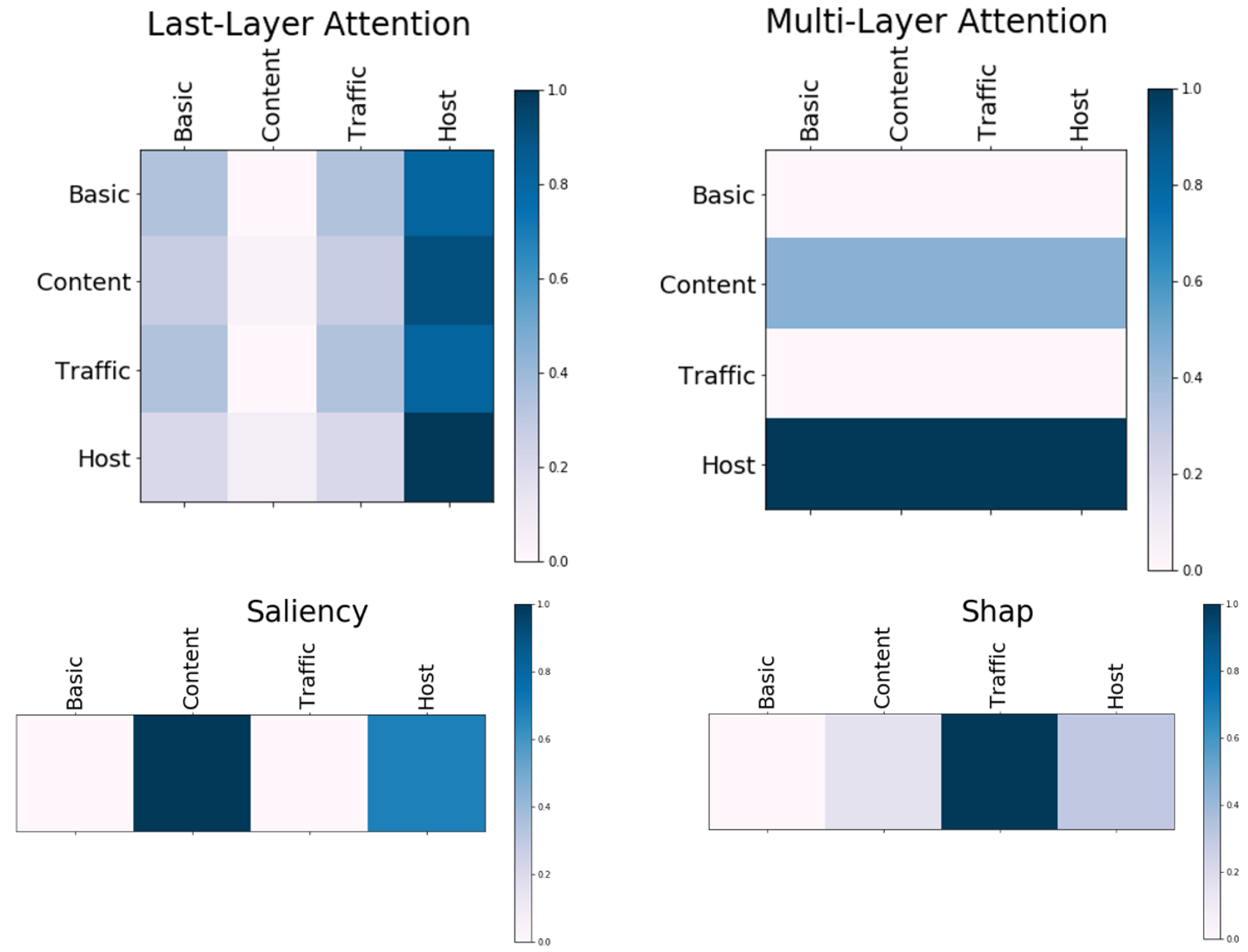
(b)

Figure 6: NI Concept groups explainability coefficients

Figures 5 and 6 show explanations corresponding to a couple of correctly classified samples from datasets CT and NI. Figure 5a shows a sample of CT where all methods identified Distances as the best concept group. This implies that the information obtained from the distances to hydrology, roadways, and fire points was identified by all methods as the most relevant for the model to conclude that the correct class was $1$. In contrast, in Figure 5b we observe a sample of class $2$ for which methods LL and MLA identified Soil Type as the best concept group, whereas SA and SH assigned larger explainability values to Distances and Generals, respectively. Similarly, two NI samples are presented in Figure 6. In Figure 6a, we observe that features related to Traffic were given larger values by all methods, yet in Figure 6b there is a lack of agreement among methods again but the two attention methods coincide.

Pairwise Method Comparison

We now contrast the results provided per method by conducting pairwise comparisons among them. To do so, we quantify the number of samples for which the selected best concept group is the same for two methods, i.e., for what percentage of the samples do two methods choose the same best concept group. The distributions of such values across the various runs are presented in Figure 7. On average, the pairwise comparisons with MLA are higher for CT and NI. As seen in Figure 7c, MLA seems to provide very different explanations to the ones generated by other methods for RW. The red square in each boxplot corresponds to the percentage of samples that chose the same best concept group when defined as the mode across all repetitions. We expected MLA and LL to have high agreement, however, this is not the case.

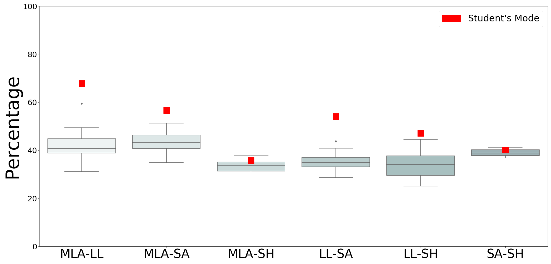
(a)

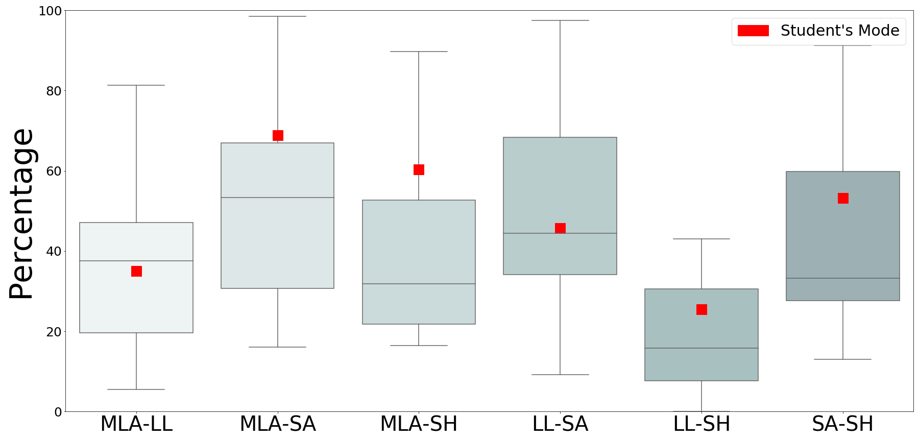
(b)

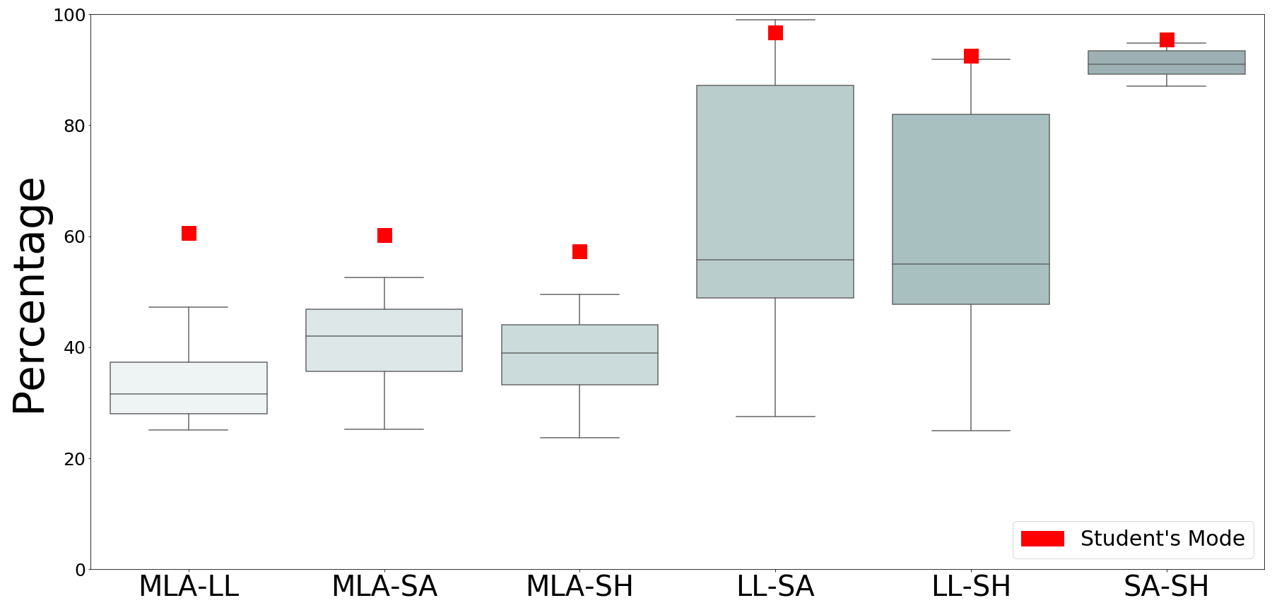
(c)

Figure 7: Best concept group pairwise comparison

As noted in the EDA, not always does a single group provide all the relevant information for a model to predict a class for a give sample. To account for this, we consider to identify the two best concept groups per method and quantify the percentage of samples where at least one of those two are the same for each pair of methods. The resulting distributions, means, and modes per pairwise comparison are reported in Figure 8.

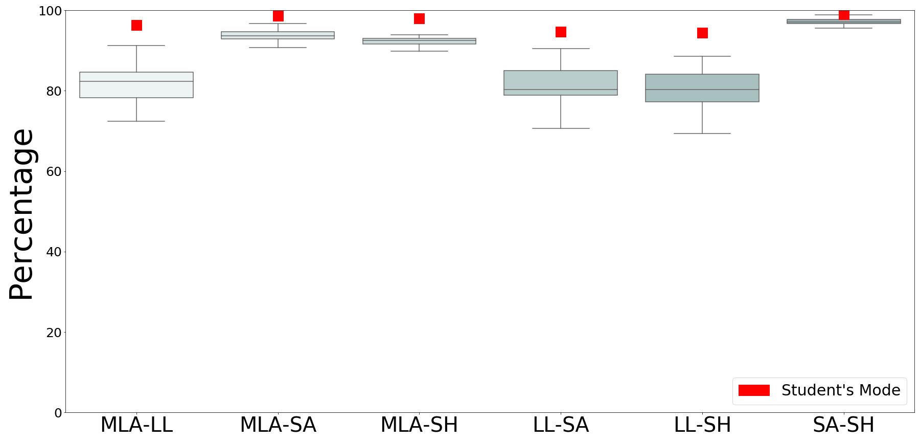
(a)

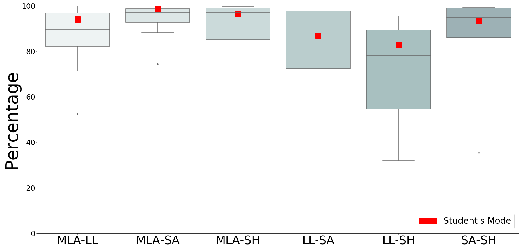
(b)

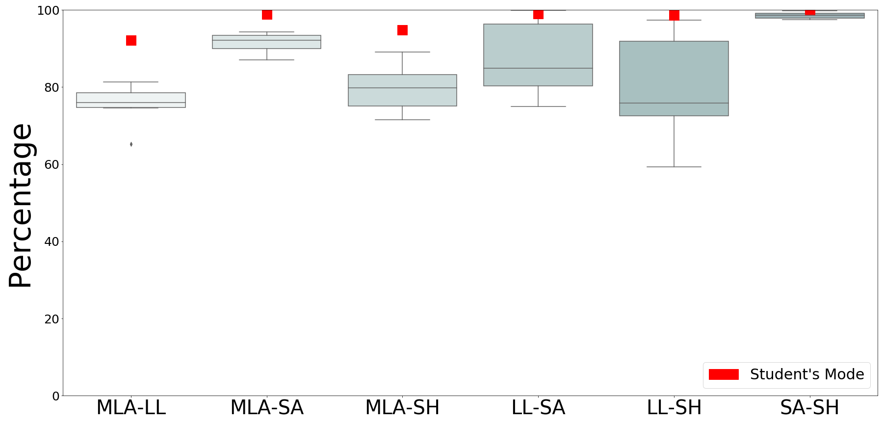
(c)

Figure 8: Two best concept groups pairwise comparison

When considering the two best concept groups, we observe very high pairwise agreement across methods. For MLA, all mean and mode pairwise overlaps are above $75\%$ and $92\%$, respectively. MLA, SA, and SH consistently show large pairwise agreements across datasets, and LL yields the smallest number of coinciding explanations.

In general, MLA shares similarities with LL, considering that MLA is also itself an attention-based method. However, across all methods, LL shows the largest variability. This seems to be improved by MLA through acknowledging attention graphs as a whole. Additionally, MLA shows better pairwise results with SA and SH than LL. On the other hand, our experiments show that gradient- and perturbation-based methods (SA and SH) are more similar to each other than to the attention-based methods. They produce similar explanations and focus mostly on a reduced number of groups (which are not necessarily different across classes) to generate explanations for predictions.

4.3.1 Stability Analysis

The stability of the explanations is analyzed by quantifying the percentage of distinct runs that agree on the same explanation for each sample. Given the previously discussed observation that SA and SH tend to steadily choose the same groups even across different samples, we focus on methods MLA and LL for this analysis. Figure 9 shows the boxplots for the best (1B) and two best (2B) concept groups per dataset.

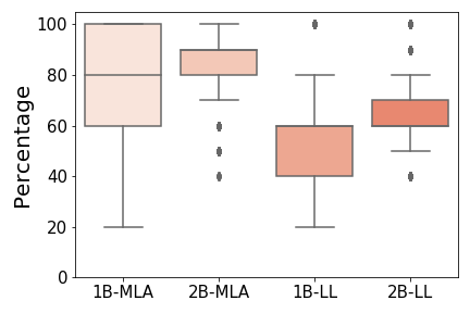
(a)

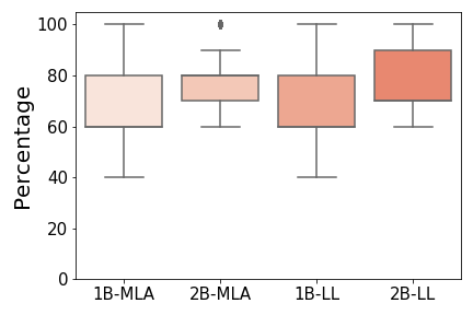
(b)

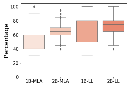
(c)

Figure 9: Percentage of runs that agree on the best (1B) and two best (2B) concept groups per method

For these datasets, the 1B concept groups comparison of MLA and LL appears inconclusive. For CT, we observe a better performance of MLA but larger variability than LL. On the other hand, the exact opposite can be said for RW, whereas both distributions seem to be identical for NI. For the 2B concept groups case, both models appear to be quite stable with averages of over $60\%$ of agreement across runs. Again, the model-to-model comparison seems to be dataset-dependant, however, MLA shows lower variability than LL. It is important to note that correlation between concept groups could have a major impact in the 1B results. In the extreme case in which the data has perfectly correlated groups, the methods are free to choose one group over the other at random. Identifying the two best concept groups helps to mitigate this issue.

5 Conclusion

In this paper, we present a novel explainability method for TD that leverages transformer models and incorporates knowledge from the graph structure of attention matrices. Combining these two, we propose a way of identifying the concept groups of input features that provide the model with the most relevant information to make a prediction. We compare our method with well-known gradient-, attention-, and perturbation-based explanations and highlight the similarities and dissimilarities observed in our experiments.

Appendix

A) Network Intrusion - Exploratory Data Analysis

B) Best Context Group Distributions by Sample Classification Output

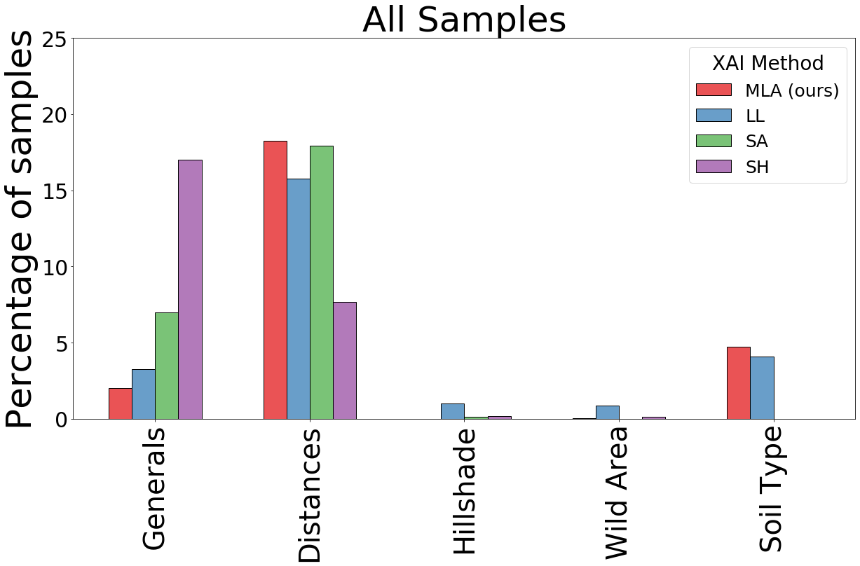
(a)

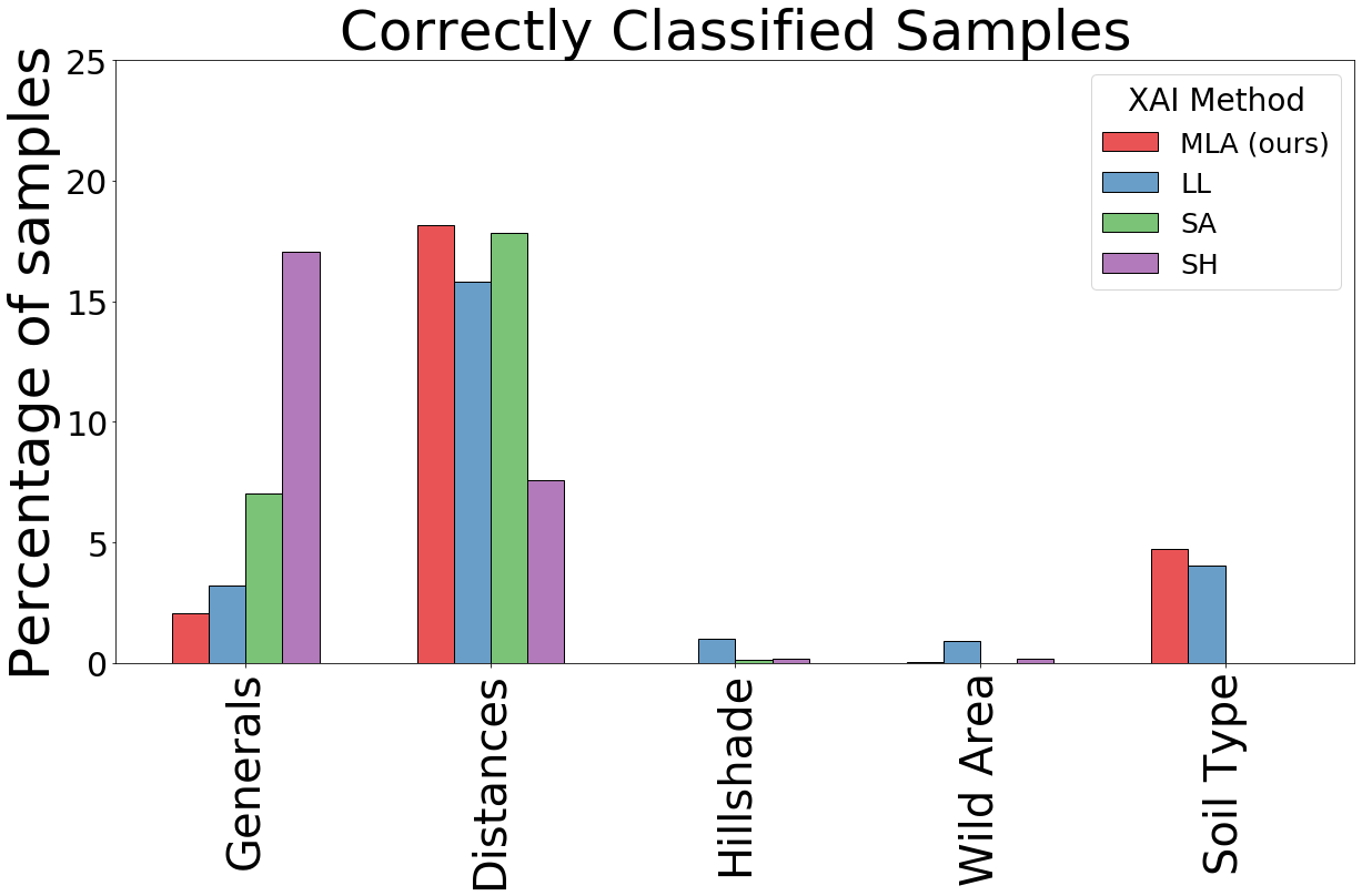
(b)

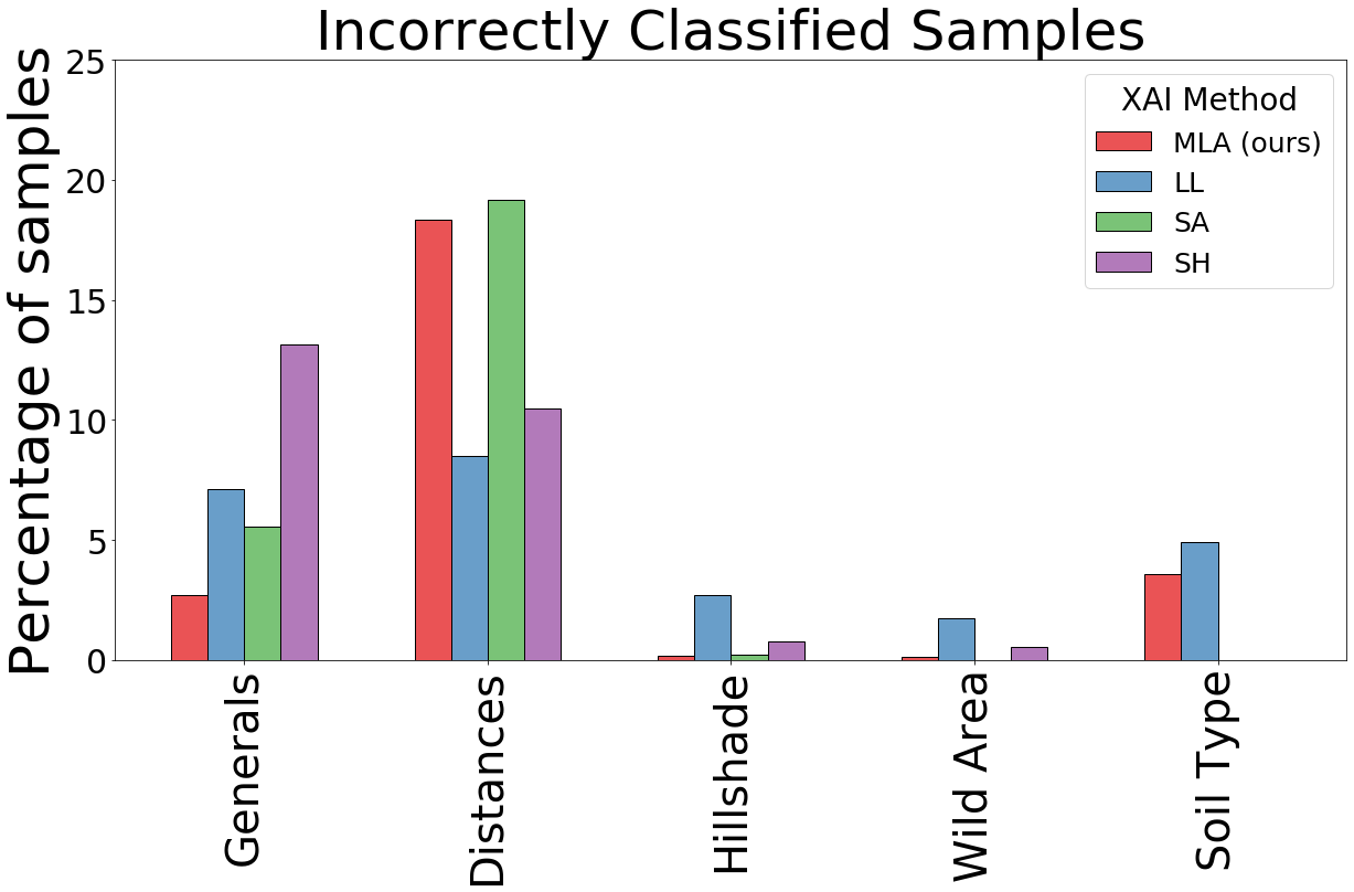
(c)

Figure 12: CT

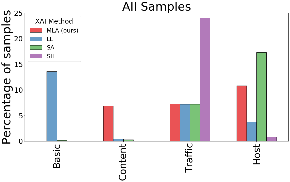
(a)

(b)

(c)

Figure 13: NI

References

- [1] P. Aggarwal and S. K. Sharma. Analysis of KDD dataset attributes - Class wise for intrusion detection. Procedia Computer Science. International Conference on Recent Trends in Computing, 2015.
- [2] S. O. Arik and T. Pfister. Tabnet: Attentive interpretable tabular learning. In Proceedings of the AAAI Conference on Artificial Intelligence, 2021.
- [3] S. Bach, A. Binder, G. Montavon, F. Klauschen, K.-R. Müller, and W. Samek. On pixel-wise explanations for non-linear classifier decisions by layer-wise relevance propagation. PLOS ONE, 2015.
- [4] J. A. Blackard. UCI Machine Learning Repository, 1999. https://archive.ics.uci.edu/ml/machine-learning-databases/covtype/covtype.info.
- [5] V. Borisov, T. Leemann, K. Seßler, J. Haug, M. Pawelczyk, and G. Kasneci. Deep neural networks and tabular data: A survey. arXiv preprint arXiv:2110.01889, 2021.
- [6] N. Carion, F. Massa, G. Synnaeve, N. Usunier, A. Kirillov, and S. Zagoruyko. End-to-end object detection with transformers. In European Conference on Computer Vision, 2020.
- [7] R. Caruana, Y. Lou, J. Gehrke, P. Koch, M. Sturm, and N. Elhadad. Intelligible models for healthcare: Predicting pneumonia risk and hospital 30-day readmission. In Proceedings of the International Conference on Knowledge Discovery and Data Mining, 2015.
- [8] H. Chefer, S. Gur, and L. Wolf. Transformer interpretability beyond attention visualization. In IEEE Conference on Computer Vision and Pattern Recognition, 2021.
- [9] R. Confalonieri, L. Coba, B. Wagner, and T. Besold. A historical perspective of explainable artificial intelligence. Wiley Interdisciplinary Reviews: Data Mining and Knowledge Discovery, 2021.
- [10] A. Das and P. Rad. Opportunities and challenges in explainable artificial intelligence (XAI): A survey. arXiv preprint arXiv:2006.11371, 2020.
- [11] E. W. Dijkstra. A note on two problems in connexion with graphs. Numerische mathematik, 1959.
- [12] I. Goodfellow, Y. Bengio, and A. Courville. Deep Learning. MIT Press, 2016. http://www.deeplearningbook.org.
- [13] Y. Gorishniy, I. Rubachev, V. Khrulkov, and A. Babenko. Revisiting deep learning models for tabular data. In Proceedings of the International Conference on Advances in Neural Information Processing Systems, 2021.
- [14] D. Gunning, M. Stefik, J. Choi, T. Miller, S. Stumpf, and G.-Z. Yang. XAI—Explainable artificial intelligence. Science Robotics, 2019.
- [15] S. Hettich and S. D. Bay. UCI KDD Archive, 1999. http://kdd.ics.uci.edu/databases/kddcup99/kddcup99.html.
- [16] G. Hinton, O. Vinyals, and J. Dean. Distilling the knowledge in a neural network. International Conference on Advances in Neural Information Processing Systems - Deep Learning and Representation Learning Workshop, 2014.
- [17] X. Huang, A. Khetan, M. Cvitkovic, and Z. S. Karnin. Tabular data modeling using contextual embeddings. 9th International Conference on Learning Representations - Workshop on Weakly Supervised Learning, 2021.
- [18] S. R. Islam, W. Eberle, S. K. Ghafoor, and M. Ahmed. Explainable artificial intelligence approaches: A survey. arXiv preprint arXiv:2101.09429, 2021.
- [19] D. P. Kingma and J. Ba. Adam: A method for stochastic optimization. 3rd International Conference for Learning Representations, 2015.
- [20] T. Lin, Y. Wang, X. Liu, and X. Qiu. A survey of transformers. AI Open, 2022.
- [21] J. Lu, D. Batra, D. Parikh, and S. Lee. ViLBERT: Pretraining task-agnostic visiolinguistic representations for vision-and-language tasks. In Proceedings of the International Conference on Advances in Neural Information Processing Systems, 2019.
- [22] S. M. Lundberg and S. I. Lee. A unified approach to interpreting model predictions. In Proceedings of the International Conference on Advances in Neural Information Processing Systems, 2017.
- [23] M. Ribeiro, S. Singh, and C. Guestrin. “Why should I trust you?”: Explaining the predictions of any classifier. In Proceedings of the Conference of the North American Chapter of the Association for Computational Linguistics: Demonstrations, 2016.
- [24] S. Roy, V. Balas, P. Samui, and S. D. Handbook of Deep Learning applications. Springer, 2019.
- [25] W. Samek, G. Montavon, A. Vedaldi, L. Hansen, and K. Müller. Explainable AI: Interpreting, explaining and visualizing Deep Learning. Lecture Notes in Computer Science. Springer, 2019.
- [26] R. R. Selvaraju, M. Cogswell, A. Das, R. Vedantam, D. Parikh, and D. Batra. Grad-cam: Visual explanations from deep networks via gradient-based localization. In IEEE International Conference on Computer Vision, 2017.
- [27] A. Shrikumar, P. Greenside, and A. Kundaje. Learning important features through propagating activation differences. In Proceedings of the International Conference on Machine Learning, 2017.
- [28] K. Simonyan, A. Vedaldi, and A. Zisserman. Deep inside convolutional networks: Visualising image classification models and saliency maps. Workshop at International Conference on Learning Representations, 2014.
- [29] D. Smilkov, N. Thorat, B. Kim, F. B. Viégas, and M. Wattenberg. SmoothGrad: Removing noise by adding noise. International Conference on Machine Learning - Workshop on Visualization for Deep Learning, 2017.
- [30] G. Somepalli, M. Goldblum, A. Schwarzschild, C. B. Bruss, and T. Goldstein. SAINT: Improved neural networks for tabular data via row attention and contrastive pre-training. arXiv preprint arXiv:2106.01342, 2021.
- [31] W. Song, C. Shi, Z. Xiao, Z. Duan, Y. Xu, M. Zhang, and J. Tang. Autoint: Automatic feature interaction learning via self-attentive neural networks. In Proceedings of the ACM International Conference on Information and Knowledge Management, 2019.
- [32] H. Tan and M. Bansal. LXMERT: Learning cross-modality encoder representations from transformers. In Proceedings of the Conference on Empirical Methods in Natural Language Processing and the 9th International Joint Conference on Natural Language Processing, 2019.
- [33] E. Tjoa and C. Guan. A survey on explainable artificial intelligence (XAI): Towards medical XAI. IEEE Transactions on Neural Networks and Learning Systems, 2021.
- [34] A. Vaswani, N. Shazeer, N. Parmar, J. Uszkoreit, L. Jones, A. N. Gomez, L. u. Kaiser, and I. Polosukhin. Attention is all you need. In Proceedings of the International Conference on Advances in Neural Information Processing Systems, 2017.
- [35] P. Veličković, G. Cucurull, A. Casanova, A. Romero, P. Liò, and Y. Bengio. Graph attention networks. International Conference on Learning Representations, 2018.
- [36] G. Vilone and L. Longo. Explainable artificial intelligence: A systematic review. arXiv preprint arXiv:2006.00093, 2020.
- [37] G. Vilone and L. Longo. Notions of explainability and evaluation approaches for explainable artificial intelligence. Information Fusion, 2021.
- [38] E. Voita, D. Talbot, F. Moiseev, R. Sennrich, and I. Titov. Analyzing multi-head self-attention: Specialized heads do the heavy lifting, the rest can be pruned. In Proceedings of the Annual Meeting of the Association for Computational Linguistics, 2019.
- [39] Q. Zhang and S. Zhu. Visual interpretability for deep learning: A survey. Frontiers of Information Technology & Electronic Engineering, 2018.