QP Chaser: Polynomial Trajectory Generation for Autonomous Aerial Tracking

Abstract

Maintaining the visibility of the targets is one of the major objectives of aerial tracking applications. This paper proposes QP Chaser, a trajectory planning pipeline that can enhance the visibility of single- and dual-target in both static and dynamic environments. As the name suggests, the proposed planner generates a target-visible trajectory via quadratic programming problems. First, the predictor forecasts the reachable sets of moving objects with a sample-and-check strategy considering obstacles. Subsequently, the trajectory planner reinforces the visibility of targets with consideration of 1) path topology and 2) reachable sets of targets and obstacles. We define a target-visible region (TVR) with topology analysis of not only static obstacles but also dynamic obstacles, and it reflects reachable sets of moving targets and obstacles to maintain the whole body of the target within the camera image robustly and ceaselessly. The online performance of the proposed planner is validated in multiple scenarios, including high-fidelity simulations and real-world experiments.

Note to Practitioners

This paper proposes an aerial target tracking framework that can be adopted in single- and dual-target scenarios. Existing approaches to keep visibility in tracking missions rarely reflect dynamic objects except for a single target. This paper suggests the prediction of the reachable area of moving objects and the generation of a target-visible trajectory, which are computed in real-time. Since the proposed planner considers the possible reach area of moving objects, generated trajectory of the drone is robust to the inaccuracy of prediction in terms of the visibility of the target. Also, the planning scheme can be extended to multiple-target scenarios.

I Introduction

Multi-rotors aided by vision sensors are widely employed in both academia [1, 2, 3, 4] and industry [5, 6, 7], due to high maneuverability and compactness of platform. The main applications of vision-aided multi-rotors are surveillance [8] and cinematography [9], and autonomous target chasing is essential in such tasks. In target-chasing missions, various situations exist in which a single drone has to handle both single- and multi-target scenarios without occlusion. For example, in filming shooting, there are scenes in that one or several actors are shot in one take, without being visually disturbed by structures in the shooting set. Moreover, the occlusion of main actors by background actors is generally prohibited. Therefore, a tracking strategy that can handle both single- and multi-target among static and dynamic obstacles can benefit various scenarios in chasing tasks.

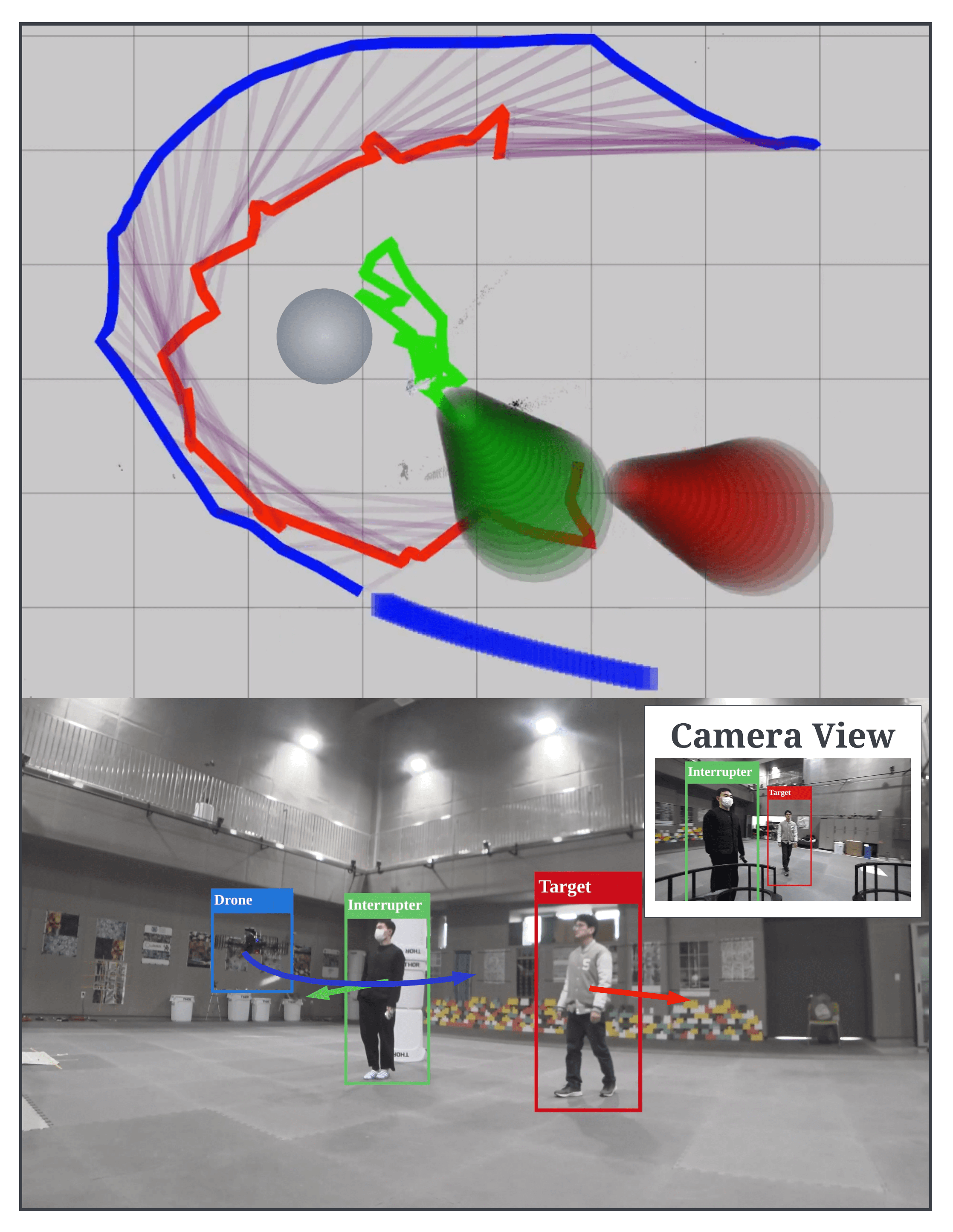
(a) Single-target tracking

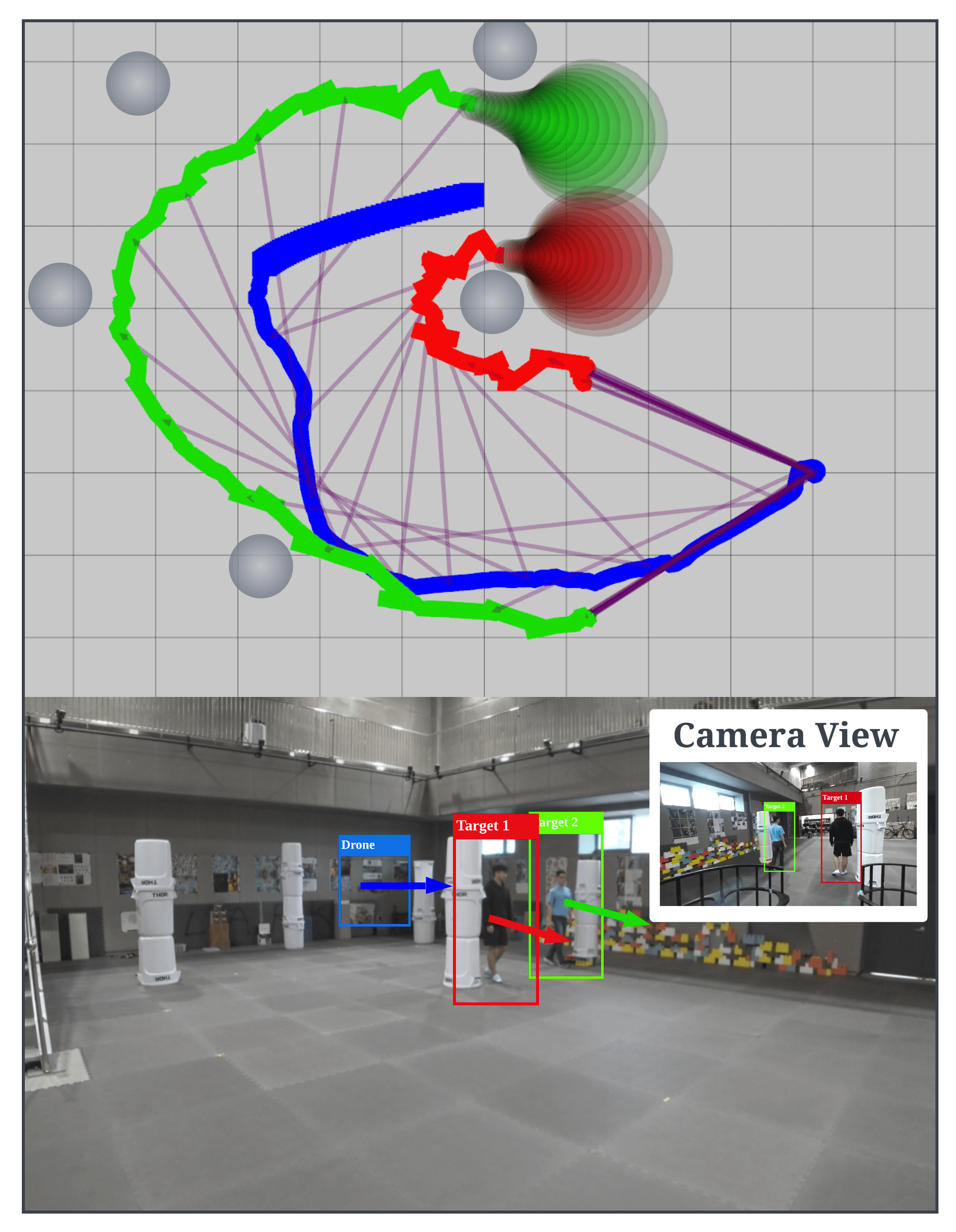
(b) Dual-target tracking

Figure 1: Target tracking mission in a realistic situation. (a): A target (red) moves in an indoor arena, and a dynamic obstacle (green) interrupts the visibility of the target. (b): Two targets (red and green) move among stacked bins (grey). A chaser drone (blue) generates a trajectory keeping the target within the camera view consistently.

Despite great attention in aerial chasing works during the recent decade, aerial target tracking remains a challenging task. First, it is difficult to forecast accurate future paths of dynamic objects due to perceptual errors from sensors and unreliable estimation of intentions of multiple moving objects in obstacle environments. Also, a motion generator in the chasing system ought to address the visibility of targets, collision avoidance against obstacles, and dynamic limits of the drone simultaneously, and should be executed in real-time.

In order to solve the problem, this paper proposes a target-chasing strategy that enhances the visibility of single- and dual-target in both static and dynamic environments. The proposed method consists of two parts: Prediction problem and Chasing problem. In the former problem, to cope with an uncertain future trajectory of the targets, the computation of reachable sets of moving objects that they can reach considering obstacle configuration is proposed. In the latter problem, we propose robustly target-visible trajectory generation that considers safety from obstacles and dynamical feasibility. The key idea of the proposed trajectory planning is a target-visible region (TVR), a time-dependent set spatial set that keeps the visibility of targets. Two-stage visibility consideration in TVR improves target visibility. First, TVR is defined based on analysis of the topology of the targets’ path to explicitly avoid inevitable target occlusion. Second, the TVR takes into account path prediction error of not only target but also dynamic obstacles. Also, to see dual-target simultaneously, the camera field of view (FOV) is additionally considered when defining TVR. In order to acquire real-time performance with the guarantee of global optimality, we formulate a chasing problem as a single quadratic programming (QP). Our main contributions are summarized as follows.

• A real-time trajectory planning framework that can handle both single and dual target-chasing missions in dynamic environments.

• A fast reachable set prediction of moving objects considering static and dynamic obstacles.

• Target-visible region (TVR) considering path topology and reachable sets of moving objects, which robustly keeps the visibility of the target.

The remainder of this paper is arranged as follows. We review the relevant references in Section II, and the relationship between visibility and topology is studied in Section III. The problem statement and a pipeline of the proposed system are presented in Section IV, and Section V describes the prediction of a reachable set of moving objects. Section VI describes TVR and design reference chasing trajectory and complete QP formulation. The validation of the proposed pipeline is demonstrated with high-fidelity simulations and real-world experiments in Section VII.

II Related Works

II-A Target Visibility among Obstacles

There have been various studies that take visibility into account in single-target chasing in static environments. [9, 10, 11] utilize nonlinear programming (NLP) to generate the chasing motion. They propose a term to penalize target occlusion in the cost function for optimization. The cost function combining multiple conflicting objectives such as actuation efficiency, collision avoidance desired shooting distance between a drone and a target, and occlusion avoidance can yield a sub-optimal solution and ruin pure tracking motion; therefore, visibility of the target is not ensured. Another line of works [12, 13] employs a cascaded structure. First, a series of safe view-points is obtained using a visibility metric that reflects Euclidean signed distance field (ESDF). Then in a subsequent module, the view-points are smoothly interpolated. However, this framework does not ensure the visibility of the target while moving between the view-points.

On the other hand, there are works that explicitly consider visibility constraints in optimization. The authors of [14, 15, 16] propose various visibility constraints and convert their problem to unconstrained optimization to generate the chasing trajectory. [14] defines visible regions and uses them in spatial-temporal trajectory optimization. [15, 16] apply a concept of path topology to enhance the robustness of visibility as in [17]. However, the above works only think of the visibility of the center of a target, not the whole body of it; hence, partial occlusion may occur while chasing the target.

Also, existing methods on target path prediction [18, 19] may generate erroneous prediction results caused by the dynamic movement of sensors and insufficient consideration of obstacles; the paths conflict with obstacles. With inaccurate target path prediction, chasing planners may not produce effective chasing paths and fail to chase a target without occlusion. Meanwhile, our framework predicts the movement of the target with consideration of obstacle configuration and generates a target-visible trajectory that is robust to prediction error.

II-B Trajectory Planning in Dynamic Environments

To the best knowledge of the authors, there are few studies considering target visibility as vital importance in dynamic environments. The approach in [20] makes a bunch of polynomial motion primitives and select the best paths that satisfy safety and visibility constraints, and it can be applied to dynamic environments. However, as target occlusion is imminent, the planner of [20] may alter the chasing path to a region with path topology, where inevitable occlusion occurred. Also, [21] designed visibility cost to address occlusion by dynamic obstacles. Since the method softly deals with occlusion, it allows the target to be hidden. On the other hand, our method directly applies concepts of the path topology to avoid inescapable occlusion and enforce strict target visibility, as in our previous work [17].

II-C Multiple Target Scenarios

Multi-target tracking frameworks with a single drone also have been discussed. The approaches in [22, 23] minimize the change in the position of the target projected on the camera image; however, they do not consider obstacle environments. A work [24] designs dual visibility score field to deal with the visibility of both targets in obstacle environments with a camera field-of-view (FOV) limit. Nevertheless, due to the fact that the designed field is made in a heuristic way; hence, the success rate of tracking missions highly depends on parameter settings. In contrast, the proposed planner considers limited camera FOV with hard constraints to ensure the simultaneous observation of the target.

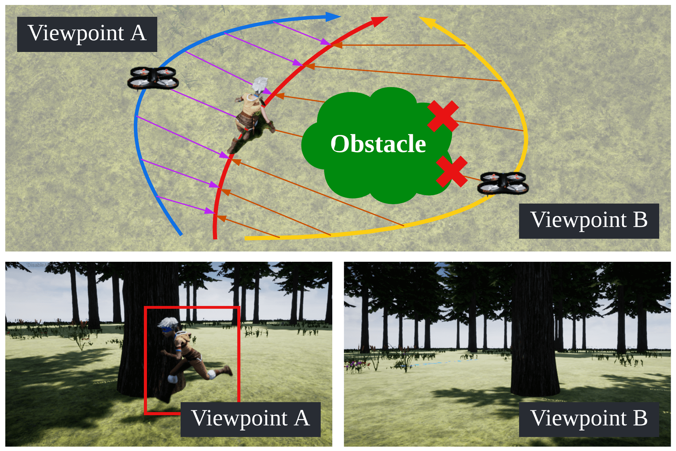
Figure 2: Comparison between two view-points. Viewpoint A can observe the target, and the path of a drone is path homotopic to the path of a target. On the contrary, the target is occluded by an obstacle at Viewpoint B, and the topology classes of the two paths are different.

III Preliminary

This section presents the relationship between target occlusion and path topology. In an obstacle environment, there exist multiple path topology classes [25]. As shown in Fig. 2, the visibility of the target is closely related to path topology. We analyzed the relation between them and reflect on the relation in generating the chasing trajectory.

As stated in [26], the definition of path homotopy is presented as the following:

Definition 1.

Paths $\sigma_{1},\sigma_{2}:I\to X\subset\mathbb{R}^{3}$ are path-homotopic if there is a continuous map $F:I\times I\to X$ such that

$$F(s,0)=\sigma_{1}(s)\ \text{and}\ F(s,1)=\sigma_{2}(s),$$ (1)

where $I$ is unit interval $[0,1]$.

In this paper, Line-of-Sight is of interest, whose definition is:

Definition 2.

Line-of-Sight is a segment connecting two objects $\textbf{x}_{1},\textbf{x}_{2}:[0,\infty)\to\mathbb{R}^{3}$.

$$L(\textbf{x}_{1}(t),\textbf{x}_{2}(t))=(1-\epsilon)\textbf{x}_{1}(t)+\epsilon\textbf{x}_{2}(t),\quad^{\forall}\epsilon\in I$$ (2)

where $t$ represents time.

Based on the definitions above, we derive a relation between the path topology and visibility between two objects.

Theorem 1.

When two objects are reciprocally visible, the paths of objects are path-homotopic.

Proof.

Suppose that two objects $\textbf{x}_{1}(t),\textbf{x}_{2}(t)$ move along paths $\sigma_{1},\sigma_{2}$ in free space $\mathcal{F}\in\mathbb{R}^{3}$ during time interval $T=[t_{0},t_{f}]$, respectively. i.e. $\sigma_{1}=\textbf{x}_{1}\circ\xi$, $\sigma_{2}=\textbf{x}_{2}\circ\xi$, where $\xi:I\to T$ is the time mapping function such that $t=\xi(s)$. If visibility between $x_{1}$ and $x_{2}$ is maintained, the Line-of-Sight does not collide with obstacles: $L(\textbf{x}_{1}(t),\textbf{x}_{2}(t))\subset\mathcal{F}$ for ${}^{\forall}t\in T$. Then, by definition, $L(\sigma_{1}(s),\sigma_{2}(s))=(1-\epsilon)\sigma_{1}(s)+\epsilon\sigma_{2}(s)\in\mathcal{F}$ for ${}^{\forall}\epsilon,s\in I$. Since such a condition satisfies the definition of continuous mapping in Definition 1, the two paths are homotopic. ∎

From Theorem 1, when the drone chooses a path with a different topology class from the target path, target occlusion inevitably occurs. Therefore, we explicitly consider path-homotopy when planning a chasing trajectory.

IV Overview

TABLE I: Nomenclature

Name	Definition
$\textbf{c}(t)$	A trajectory of the drone. $\textbf{c}(t)\in\mathbb{R}^{2}$
$\underline{\textbf{c}}$	An optimization variable that consists of Bernstein coefficients representing $\textbf{c}(t)$.
$n_{c}$	The degree of a polynomial trajectory $\textbf{c}(t)$.
$T$	Planning horizon
$\theta_{f}$	FOV of the camera built on the drone.
$v_{\text{max}},a_{\text{max}}$	The maximum speed and acceleration of the drone.
$\boldsymbol{\mathcal{O}},\mathcal{O}_{i}$	A set of obstacles. An $i$-th obstacle in $\mathcal{O}$
$N_{o},N_{samp}$	The number of elements of $\mathcal{O}$ and samples of end-points in the prediction.
$\mathcal{R}_{q_{i}}(t),\hat{\textbf{q}}_{i}(t),r_{q_{i}}(t)$	A reachable set of an $i$-th target. A predicted center trajectory and radius of $\mathcal{R}_{q_{i}}(t)$. We omit a subscript $i$ to handle an arbitrary target.
$\mathcal{R}_{o_{i}}(t),\hat{\textbf{o}}_{i}(t),r_{o_{i}}(t)$	A reachable set of an $i$-th obstacle. A predict center trajectory and radius of $\mathcal{R}_{o_{i}}(t)$. We omit a subscript $i$ to handle an arbitrary target.
$L(\textbf{x}_{1},\textbf{x}_{2})$	Line-of-Sight between $\textbf{x}_{1}$ and $\textbf{x}_{2}$.
$\mathcal{V}_{O}(t),\mathcal{V}_{F}(t)$	Target visible region (TVR) against an obstacle and considering camera FOV.
${}_{\textbf{x}_{2}}\textbf{x}_{1}(t)$	Relative position between $\textbf{x}_{1}(t)$ and $\textbf{x}_{2}(t)$. $\textbf{x}_{1}(t)-\textbf{x}_{2}(t)$.
$\|\textbf{x}\|_{p},{\textbf{x}}^{(i)}(t)$	$L_{p}$ norm of x. $i$-th time derivative of $\textbf{x}(t)$.
$\textbf{x}_{x},\textbf{x}_{y}$	$x$- and $y$-components of x.
$\begin{pmatrix}n\\ k\end{pmatrix}$	Binomial coefficients, the number of $k$-combinations from a set of $n$ elements.
$\textbf{0}_{m\times n}$	An $m\times n$ matrix with all-zero elements.
$I_{m\times m}$	An identity matrix with rank $m$.
$\text{det}(\cdot)$	Determinant of a matrix.
$\mathcal{B}(\textbf{x},r)$	A ball with center at x and radius $r$.
$\partial\mathcal{A}$	A boundary of a closed set $\mathcal{A}$.
$\overline{AB}$, $\angle{ABC}$	Segment connecting points $A$ and $B$. Angle between $\overline{BA}$ and $\overline{BC}$.

IV-A Problem Setup

In this section, we formulate the trajectory planning problem for a tracking drone with firmly attached camera sensors having limited FOV $\theta_{f}\in(0,\pi)$ [rad]. Our goal is to generate a trajectory of the drone that can see the single- and dual-target ceaselessly in an obstacle environment $\mathcal{W}$ over the time horizon $[0,T]$. To achieve the goal, the drone has to predict the future motions of moving objects like the target and dynamic obstacles, and the planner generates a continuous-time trajectory of the drone that keeps the visibility of the target while satisfying dynamical feasibility and avoiding a collision. To accomplish the missions, we set up two problems: 1) Prediction problem and 2) Chasing problem.

We assume that the environment $\mathcal{W}$ consists of separate cylindrical static and dynamic obstacles, and a set of obstacles is denoted as $\mathcal{O}$. In addition, flying at a higher altitude may provide a simple solution for target tracking missions, but we set the flying height of the drone to a fixed level for the acquisition of consistent images of the target. From the problem settings, we focus on the design of chasing trajectory in the $x-y$ plane.

Throughout this article, we use the notation in Table I. The bold small letters represent a vector, calligraphic capital letters denote a set, and italic small letters mean scalar value.

IV-A1 Prediction problem

The prediction module forecasts reachable sets of moving objects such as targets and dynamic obstacles, over a time horizon $t\in[0,T]$. The reachable set $\mathcal{R}_{\textbf{p}}(t)$ is a set that moving objects can reach and has to be set considering an obstacle set $\mathcal{O}$ as well as estimation error. The goal is to calculate $\mathcal{R}_{\textbf{p}}(t)$ enveloping the possible future position of the moving objects $\textbf{p}(t)$. In this paper, using q and o instead of p represent information of reachable sets of the target and obstacles, respectively. Specifically, we represent the $i$-th target ,$i=1,2$, and $j$-th obstacle $j=\{1,\ldots,N_{o}:=|\mathcal{O}|\}$, as $\textbf{q}_{i}$, $\textbf{o}_{j}$ respectively.

IV-A2 Chasing problem

Given the reachable sets of the target and the obstacles obtained by the prediction module, we generate a trajectory of the drone $\textbf{c}(t)$ that keeps the visibility of the target (3b), does not collide with obstacles (3c), and satisfies dynamical limits (3d), (3e). For the smoothness of the trajectory and high visibility, the cost function (3a) consists of terms penalizing jerky motion $J_{j}$ and tracking error to designed reference trajectory $J_{e}$. We formulate a tracking problem as

$$\underset{\textbf{c}(t)}{\text{min}} J=w_{j}J_{j}+w_{e}J_{e}$$ (3a)

s.t. $$L(\textbf{c}(t),\mathcal{R}_{\textbf{q}}(t))\subset\mathcal{F}\setminus\mathcal{R}_{\textbf{o}}(t)$$ (3b)

$$\mathcal{B}(\textbf{c}(t),r_{c})\subset\mathcal{F}\setminus\big{\{}\bigcup_{i=1}^{N_{o}}\mathcal{R}_{\textbf{o}_{i}}(t)\cup\mathcal{R}_{\textbf{q}}(t)\big{\}}$$ (3c)

$$\textbf{c}^{(i)}(0)=\textbf{c}^{(i)}_{0},\ i=0,1$$ (3d)

$$\|\textbf{c}^{(1)}(t)\|_{2}\leq v_{\text{max}},\ \|\textbf{c}^{(2)}(t)\|_{2}\leq a_{\text{max}}$$ (3e)

where $w_{j}$ and $w_{e}$ are weight factors of the costs, $r_{c}$ is radius of the drone, and $\textbf{c}^{(i)}_{0},i=0,1$ are current position and velocity of the drone.

IV-A3 Assumptions

The stated problems are to be solved along with the below assumptions. For the Prediction Problem, we assume that P1) the moving objects do not collide with obstacles, and P2) they do not move in a jerky way. In the Chasing Problem, we assume that C1) the maximum velocity $v_{\text{max}}$ and the maximum acceleration $a_{\text{max}}$ are higher than the target and obstacles, and C2) the current state of drone does not violate (3b)-(3e). Furthermore, based on Theorem 1, when the targets move along paths with different path topology, occlusion unavoidably occurs, so we assume that C3) all targets move along homotopic paths against obstacles.

IV-A4 Trajectory representation

Due to the virtue of differential flatness of quadrotor dynamics [27], the trajectory of multi-rotors can be expressed with a polynomial function of time $t$. In this paper, Bernstein basis is deployed to express polynomials. Bernstein bases of $n$-th order polynomial for time interval $[t_{a},t_{b}]$ are defined as follows:

$$B_{k,n}(t,t_{a},t_{b})=\begin{pmatrix}n\\ k\end{pmatrix}\frac{(t_{b}-t)^{n-k}(t-t_{a})^{k}}{(t_{b}-t_{a})^{n}},\ 0\leq k\leq n$$ (4)

Since the bases defined above are non-negative in the time interval $[t_{a},t_{b}]$, a linear combination with non-negative coefficients makes the total value become non-negative. We utilize this property in the following sections.

The trajectory of the chasing drone, $\textbf{c}(t)=[c_{x}(t),c_{y}(t)]^{T}\in\mathbb{R}^{2}$, is represented as an $M$-segment piecewise Bernstein polynomial:

$$\textbf{c}(t)=\begin{cases}&\textbf{C}_{1}^{T}\textbf{B}_{n_{c},1}(t)\ \ \ \ \ t\in[T_{0},T_{1}]\\ &\textbf{C}_{2}^{T}\textbf{B}_{n_{c},2}(t)\ \ \ \ \ t\in[T_{1},T_{2}]\\ &\ldots\\ &\textbf{C}_{M}^{T}\textbf{B}_{n_{c},M}(t)\ \ \ t\in[T_{M-1},T_{M}]\\ \end{cases}$$ (5)

where $T_{0}=0$ (current time), $T_{M}=T$, $n_{c}$ is the degree of polynomial, $\textbf{C}_{i}=[\textbf{c}_{i(x)},\textbf{c}_{i(y)}]\in\mathbb{R}^{(n_{c}+1)\times 2}$ and $\textbf{B}_{n_{c},i}(t)=[B_{0,n_{c}}(t,T_{0},T_{1}),\ldots,B_{n_{c},n_{c}}(t,T_{M-1},T_{M})]^{T}$ are control points and the corresponding basis vector of the $i$-th segment, respectively. An array of control points in the $i$-th segment is defined as $\textbf{c}_{i}=[\textbf{c}_{i(x)}^{T},\textbf{c}_{i(y)}^{T}]^{T}\in\mathbb{R}^{2(n_{c}+1)}$, and a concatenated vector of all control points $\underline{\textbf{c}}=[\textbf{c}_{1}^{T},\ldots,\textbf{c}_{M}^{T}]^{T}\in\mathbb{R}^{2M(n_{c}+1)}$ is a decision vector of the polynomial trajectory optimization.

IV-A5 Objectives

For the Prediction Problem, the prediction module forecasts moving objects’ reachable set $\mathcal{R}_{\textbf{p}}(t)$. Then, for the Chasing Problem, the chasing module formulates a QP problem with respect to $\underline{\textbf{c}}$ and finds an optimal $\underline{\textbf{c}}$ so that the drone chases the target without occlusion and collision while satisfying dynamical limits.

IV-B Pipeline

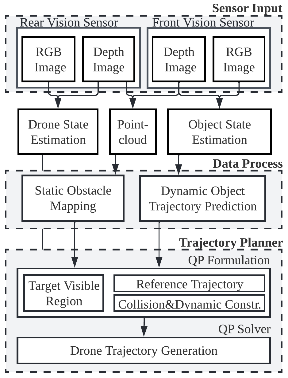
Figure 3: Pipeline of the proposed chasing system.

The proposed overall architecture of QP Chaser is shown in Fig. 3. From camera sensors, RGB and depth images are acquired, and point cloud and information of target poses are extracted from the images. Then, locations and dimensions of static obstacles are estimated from the point cloud to build an obstacle map, and the reachable sets of the target and dynamic obstacles are predicted based on observed poses of the dynamic obstacles and the targets. Based on the static obstacle map and prediction results, the chasing trajectory generation is executed.

V Object Trajectory Prediction

From the observation by camera sensors, position, velocity, and their estimation error covariance, and dimension (radius) of moving objects are acquired as $\hat{\textbf{p}}_{0}$, $\hat{\textbf{p}}^{(1)}_{0}$, $P_{0}$, and $r_{p0}$ at current time $t=0$, respectively. We first sample the position that can be reached with the current dynamical state at $t=T$ and generate motion primitives which can represent the possible trajectory of the moving objects. Then, we filter out the primitives that collide with obstacles and define a reachable set $\mathcal{R}_{\textbf{p}}(t)$ that encloses the non-conflicting primitives.

V-A Candidate for Future Trajectory of Moving Object

V-A1 End point sampling

We first estimate the position of a moving object at time $t=T$. Moving object dynamics can be modeled as a constant velocity model with disturbance and is represented as

$$\begin{bmatrix}\textbf{p}^{(1)}(t)\\ \textbf{p}^{(2)}(t)\end{bmatrix}=F_{p}\begin{bmatrix}\textbf{p}(t)\\ \textbf{p}^{(1)}(t)\end{bmatrix}+G_{p}\textbf{w},\quad\textbf{w}\sim(0,Q),$$ (6)

$$F_{p}=\begin{bmatrix}\textbf{0}_{2\times 2}&\textbf{I}_{2\times 2}\\ \textbf{0}_{2\times 2}&\textbf{0}_{2\times 2}\end{bmatrix},\quad G_{p}=\begin{bmatrix}\textbf{0}_{2\times 2}\\ \textbf{I}_{2\times 2}\end{bmatrix}$$

where $\textbf{p}(t)$ is position of the moving object, and $\textbf{w}\in\mathbb{R}^{2}$ is white noise with covariance $Q$. Then prediction error covariance $P(t)$ propagates along with time and is represented as

$$P^{(1)}(t)=F_{p}(t)P(t)+P(t)F_{p}^{T}(t)+G_{p}QG_{p}^{T}$$ (7)

(7) is differential Ricatti equation and error propagation matrix $P(t)$ can be calculated algebraically.
We sample $N_{samp}$ points from a 2-dimensional gaussian distribution $\mathcal{N}(\int_{0}^{T}e^{-F_{p}(T-\tau)}[\hat{\textbf{p}}_{0}^{T},\hat{\textbf{p}}_{0}^{(1)T}]^{T}d\tau,P(T))$ and call a set of the samples End Point Set and represent it as

$$\mathcal{S}_{p}=\{\textbf{s}_{p,i}\in\mathbb{R}^{2}|i=1,\ldots,N_{samp}\}$$ (8)

V-A2 Primitive generation

Given the initial position, velocity, and end positions, we design trajectory candidates for moving objects. Under the assumption P2) that moving objects do not move in a jerky way, we establish the following problem.

$$\underset{\hat{\textbf{p}}(t)}{\text{min}} \int_{0}^{T}\|\hat{\textbf{p}}^{(3)}(t)\|^{2}_{2}dt$$ (9)

s.t. $$\hat{\textbf{p}}(0)=\hat{\textbf{p}}_{0},\ \hat{\textbf{p}}^{(1)}(0)=\hat{\textbf{p}}^{(1)}_{0},\ \hat{\textbf{p}}(T)\in\mathcal{S}_{p}$$

Recalling that the trajectory is represented with Bernstein polynomial, we write an $i$-th candidate trajectory, that satisfies $\hat{\textbf{p}}(T)=\textbf{s}_{p,i}$, as $\hat{\textbf{p}}_{i}(t)=\textbf{P}^{T}_{i}\boldsymbol{B}_{n_{p}}(t)$, $i=1,\ldots,N_{samp}$ where $\textbf{P}_{i}=[\textbf{p}_{i(x)},\textbf{p}_{i(y)}]\in\mathbb{R}^{(n_{p}+1)\times 2}$ and $\boldsymbol{B}_{n_{p}}(t)=[B_{0,n_{p}}(t,0,T),\ldots,B_{n_{p},n_{p}}(t,0,T)]^{T}$. By defining $\textbf{p}_{i}:=[\textbf{p}_{i(x)}^{T},\textbf{p}_{i(y)}^{T}]^{T}$ as an optimization variable, (9) become a QP problem as

$$\underset{\textbf{p}_{i}}{\text{min}} \frac{1}{2}\textbf{p}_{i}^{T}Q_{p}\textbf{p}_{i}$$ (10)

s.t. $$A_{p}\textbf{p}_{i}=\textbf{b}_{p,i}$$

where $Q_{p}$ is a positive semi-define matrix, $A_{p}$ is a $6$ by $(n_{p}+1)$ matrix, and $\textbf{b}_{p,i}$ is a vector composed of $\hat{\textbf{p}}_{0}$, $\hat{\textbf{p}}^{(1)}_{0}$, and $\textbf{s}_{p,i}$. (10) can be converted into unconstrained QP, and the optimal $\textbf{p}_{i}$ is a closed solution as follows.

$$\begin{bmatrix}\textbf{p}_{i}\\ \boldsymbol{\lambda}\end{bmatrix}=\begin{bmatrix}Q_{p}&A_{p}^{T}\\ A_{p}&\textbf{0}_{6\times 6}\end{bmatrix}^{-1}\begin{bmatrix}\textbf{0}_{2(n_{p}+1)\times 1}\\ \textbf{b}_{p,i}\end{bmatrix}$$ (11)

where $\boldsymbol{\lambda}$ is a lagrange multiplier. A set of candidate trajectories of the moving object is defined as follows

$$\mathcal{P}_{p}=\{\hat{\textbf{p}}_{i}(t)|\hat{\textbf{p}}_{i}(t)=\textbf{P}^{T}_{i}\boldsymbol{B}_{n_{p}}(t),\ i=1,\ldots,N_{samp}\}$$ (12)

V-B Collision Check

Under the assumption P1) that moving objects do not collide, trajectory candidates $\hat{\textbf{p}}_{i}(t)\in\mathcal{P}_{p}$ that violate the condition $\|\hat{\textbf{p}}_{i}(t)-\textbf{o}_{j}(t)\|_{2}^{2}-(r_{p0}+r_{o_{j}}(t))^{2}\geq 0,$ $(\forall t\in[0,T])$ are filtered out. Due to the fact that all terms in the non-colliding condition are represented in polynomials, and Bernstein bases are non-negative in the time period $[0,T]$, whole non-negative coefficients make the left-hand side non-negative. We examine all coefficients of each basis of $\forall\hat{\textbf{p}}_{i}(t)\in\mathcal{P}_{p}$ and select the primitives which have all non-negative coefficients. For details, see Appendix.A. A set of primitives that pass the test is defined as $\mathcal{P}_{s}$.

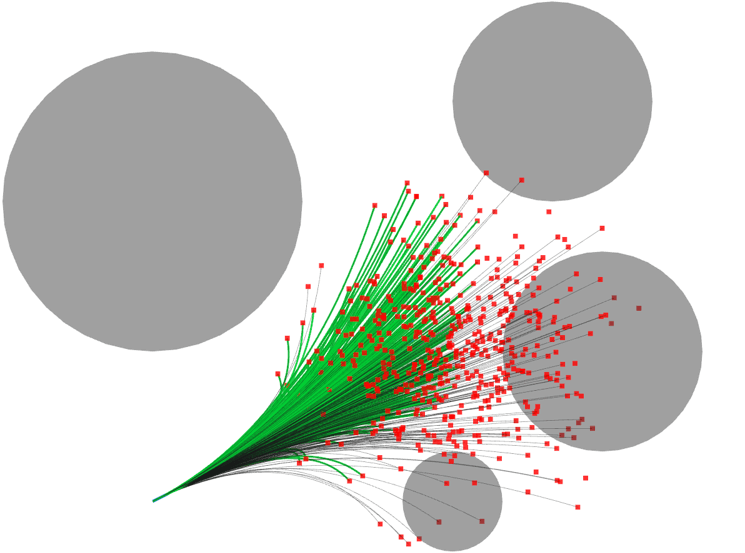
(a)

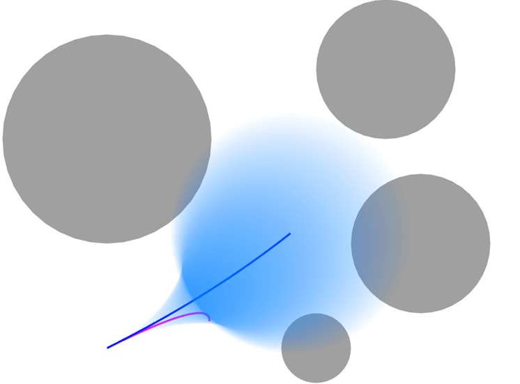
(b)

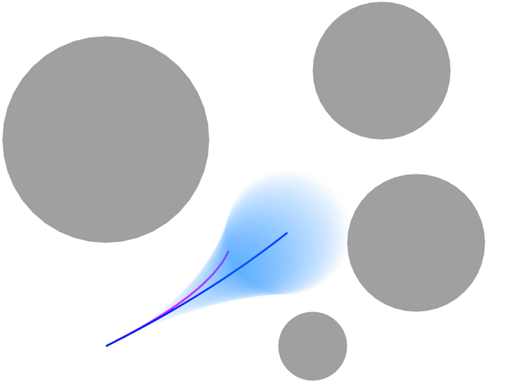
(c)

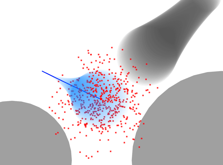
(d)

Figure 4: (a): Sampled endpoints (red), primitives $\mathcal{P}_{p}$ (black), and safe primitives $\mathcal{P}_{s}$ (green) among obstacles (grey). (b): The best primitive $\hat{\textbf{p}}(t)$ (blue), reachable set $\mathcal{R}_{\textbf{p}}(t)$ (light blue), and the farthest primitive $\hat{\textbf{p}}^{\prime}(t)$ (magenta) for moving objects. (c): The prediction with $\epsilon_{p}=0.2$. (d): The prediction in a dynamic environment.

TABLE II: Computation time in Prediction Process

$(N_{samp},N_{o})$	(500,2)	(500,4)	(2000,2)	(2000,4)
Sampling End Points & Primitive Generation [$\mu$s]	43.97	47.23	168.3	184.1
Collision Check [$\mu$s]	146.3	185.3	487.9	750.7
Reachable Set Computation [ms]	0.245	0.172	2.921	2.073
Total Time [ms]	0.435	0.405	3.577	3.008

V-C Prediction with Error Bounds

With the set of non-colliding primitives $\mathcal{P}_{s}$, the reachable set $\mathcal{R}_{\textbf{p}}(t)$ with the following representation is defined.

$$\mathcal{R}_{\textbf{p}}(t)=\mathcal{B}(\hat{\textbf{p}}(t),r_{p}(t))$$ (13)

We determine the primitive having the smallest sum of distance with the other primitives as a center trajectory $\hat{\textbf{p}}(t)$, which is expressed as follows.

$$\hat{\textbf{p}}(t)=\underset{\hat{\textbf{p}}_{i}(t)\in\mathcal{P}_{s}}{\text{argmin}}\sum_{j\neq i}\int_{0}^{T}\|\hat{\textbf{p}}_{i}(t)-\hat{\textbf{p}}_{j}(t)\|_{2}dt$$ (14)

Proposition 1.

The optimization problem (14) is equivalent to the following problem.

$$\hat{\textbf{p}}(t)=\hat{\textbf{p}}_{i^{*}}(t),\ i^{*}=\underset{i}{\text{argmin}}\sum_{j=0}^{|\mathcal{P}_{p}|}\|\textbf{s}_{p,i}-\textbf{s}_{p,j}\|_{2},$$ (15)

$$\text{where}\ i\neq j\in\{1,\ldots,|\mathcal{P}_{p}|\}\ \wedge\ \hat{\textbf{p}}_{i}(t),\hat{\textbf{p}}_{j}(t)\in\mathcal{P}_{s}$$

Proof.

See Appendix B. ∎

From Proposition 1, $\hat{\textbf{p}}(t)$ is determined by simple arithmetic operations and a min algorithm with time complexity $O(|\mathcal{P}_{s}|^{2})$ and $O(|\mathcal{P}_{s}|)$, respectively. Then we define $r_{p}(t)$ so that $\mathcal{R}_{\textbf{p}}(t)$ encloses all primitives in $\mathcal{P}_{s}$ for $\forall{t}\in[0,T]$.

$$r_{p}(t)=\|\hat{\textbf{p}}(t)-\hat{\textbf{p}}^{\prime}(t)\|_{2}+r_{p0},$$ (16)

$$\text{where}\ \hat{\textbf{p}}{{}^{\prime}}(t)=\underset{\hat{\textbf{p}}_{i}(t)\in\mathcal{P}_{s}}{\text{argmax}}\int_{0}^{T}\|\hat{\textbf{p}}(t)-\hat{\textbf{p}}_{i}(t)\|_{2}^{2}dt$$

V-D Evaluation

Fig. 4 visualizes the prediction process among multiple obstacles. We set $n_{p}$ as a minimum degree 3 and test 1000 times for different scenarios $(N_{samp},N_{o})$ $=(500,2),(500,4),(2000,2),(2000,4)$. The prediction module is computed on a laptop with Intel i7 CPU, with a single thread implementation, and execution time is summarized in Table. II. During the entire test, $\textbf{p}(t)\in\mathcal{R}_{\textbf{p}}(t)$, $\forall t\in[0,T]$ was satisfied with a empirical probability 0.988.

VI Chasing Trajectory Generation

In the previous section, we focused on the prediction of the reachable set of moving objects: the target $\mathcal{R}_{\textbf{q}}(t)=\mathcal{B}(\hat{\textbf{q}}(t),r_{q}(t))$, and obstacles $\mathcal{R}_{\textbf{o}}(t)=\mathcal{B}(\hat{\textbf{o}}(t),r_{o}(t))$. This section formulates a QP problem with respect to optimization variable $\underline{\textbf{c}}$, that represents Chasing Problem.

VI-A Topology Check

In 2-dimensional space, there exist two classes of path topology against a single obstacle as shown in Fig. 2, and as stated in Theorem 1, the drone should move along a homotopic path with the target path to avoid occlusion. Based on the relative position between the drone and the obstacle, ${}_{\hat{\textbf{o}}}\textbf{c}(t)=\textbf{c}(t)-\hat{\textbf{o}}(t)$, and the relative position between the target and the obstacle, ${}_{\hat{\textbf{o}}}\hat{\textbf{q}}(t)=\hat{\textbf{q}}(t)-\hat{\textbf{o}}(t)$, at the current time $t=0$, the topology class of chasing path is determined as follows.

$$\begin{cases}&\textit{Class O1}\ (\text{if}\ \det\begin{bmatrix}{}_{\hat{\textbf{o}}}\textbf{c}^{T}(0)\\ {}_{\hat{\textbf{o}}}\hat{\textbf{q}}^{T}(0)\end{bmatrix}\geq 0)\\ &\textit{Class O2}\ (\text{if}\ \det\begin{bmatrix}{}_{\hat{\textbf{o}}}\textbf{c}^{T}(0)\\ {}_{\hat{\textbf{o}}}\hat{\textbf{q}}^{T}(0)\end{bmatrix}<0)\\ \end{cases}$$ (17)

Based on the topology check above, the visibility constraint and reference chasing trajectory are defined.

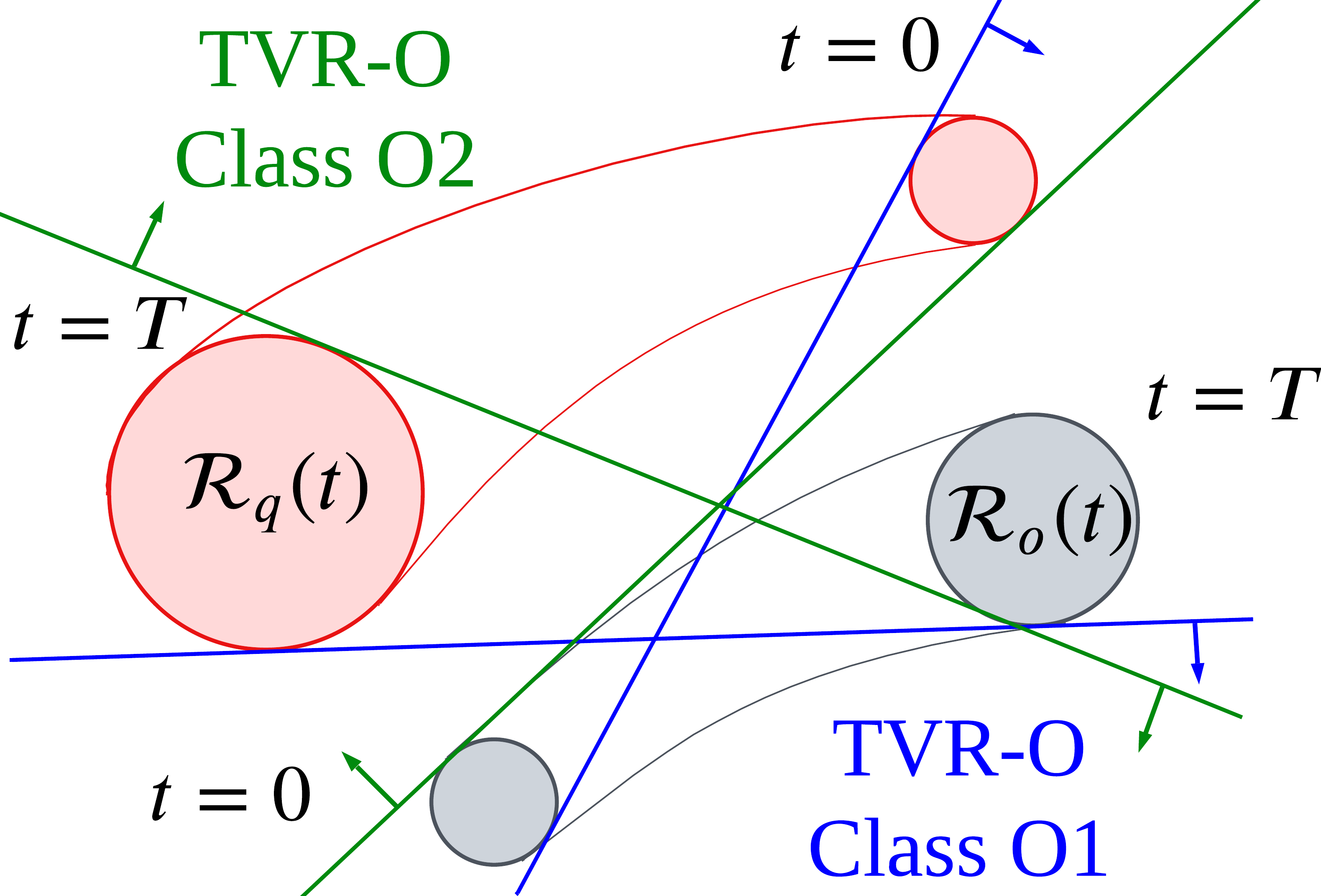
(a)

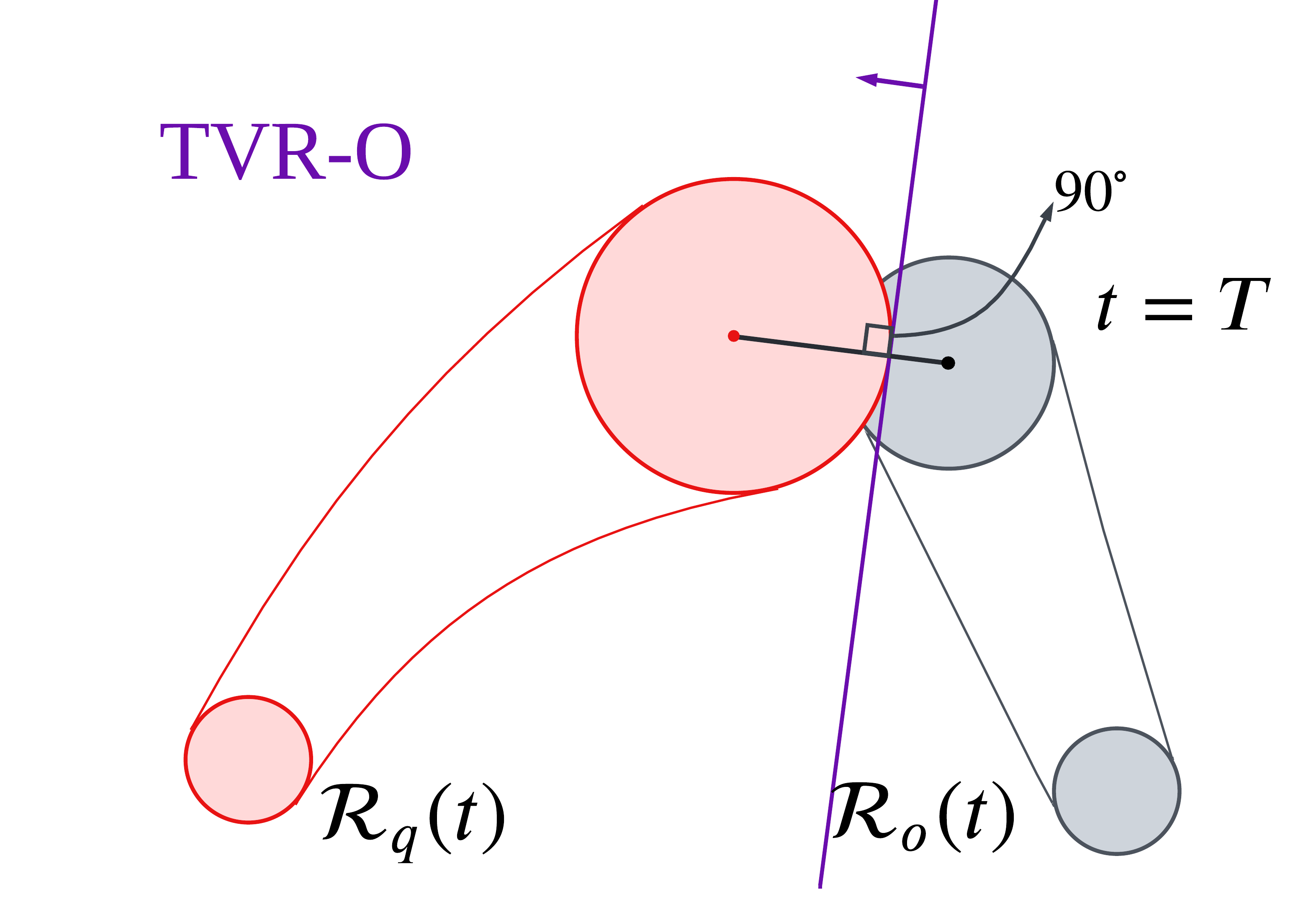
(b)

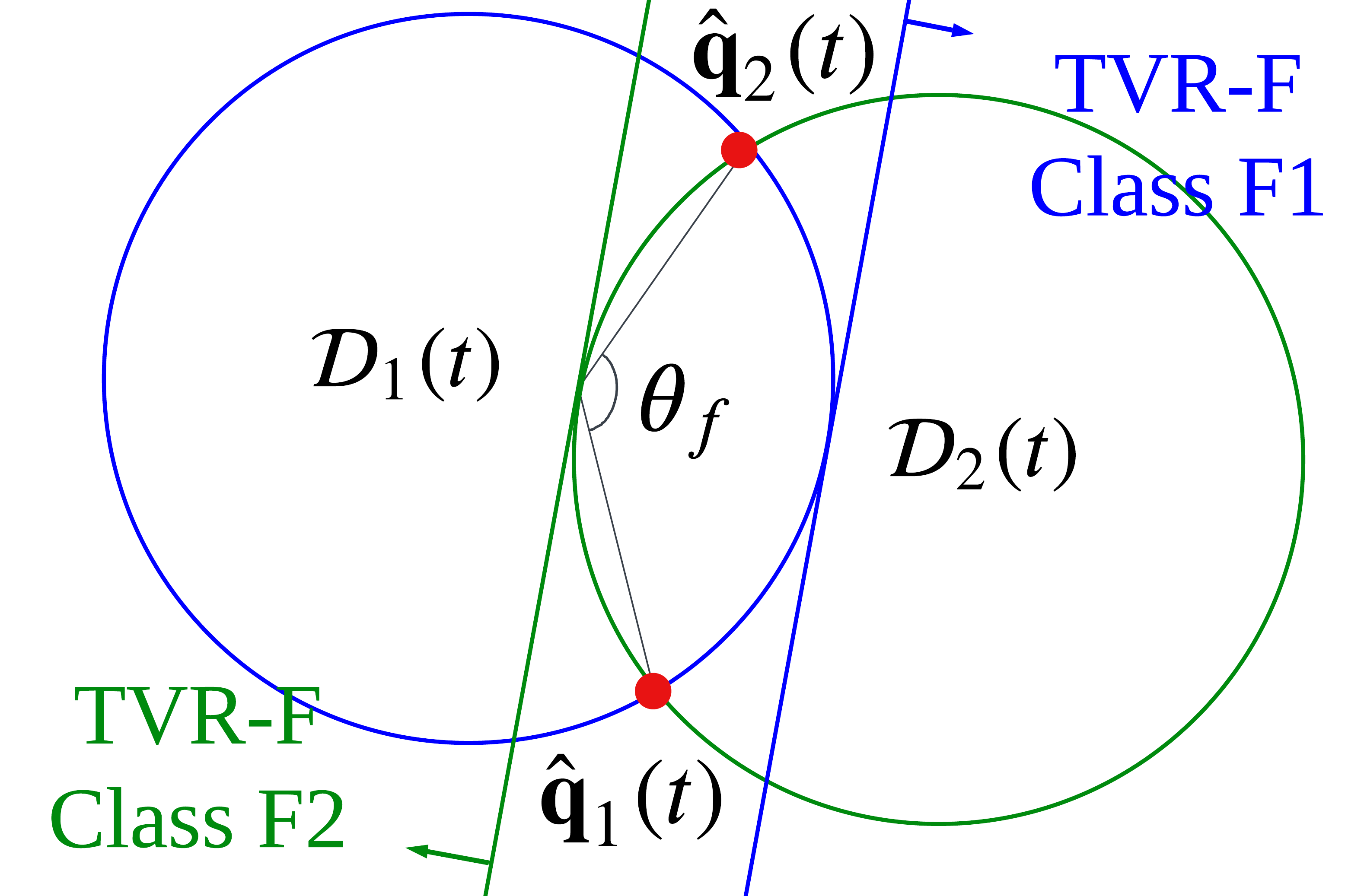
(c)

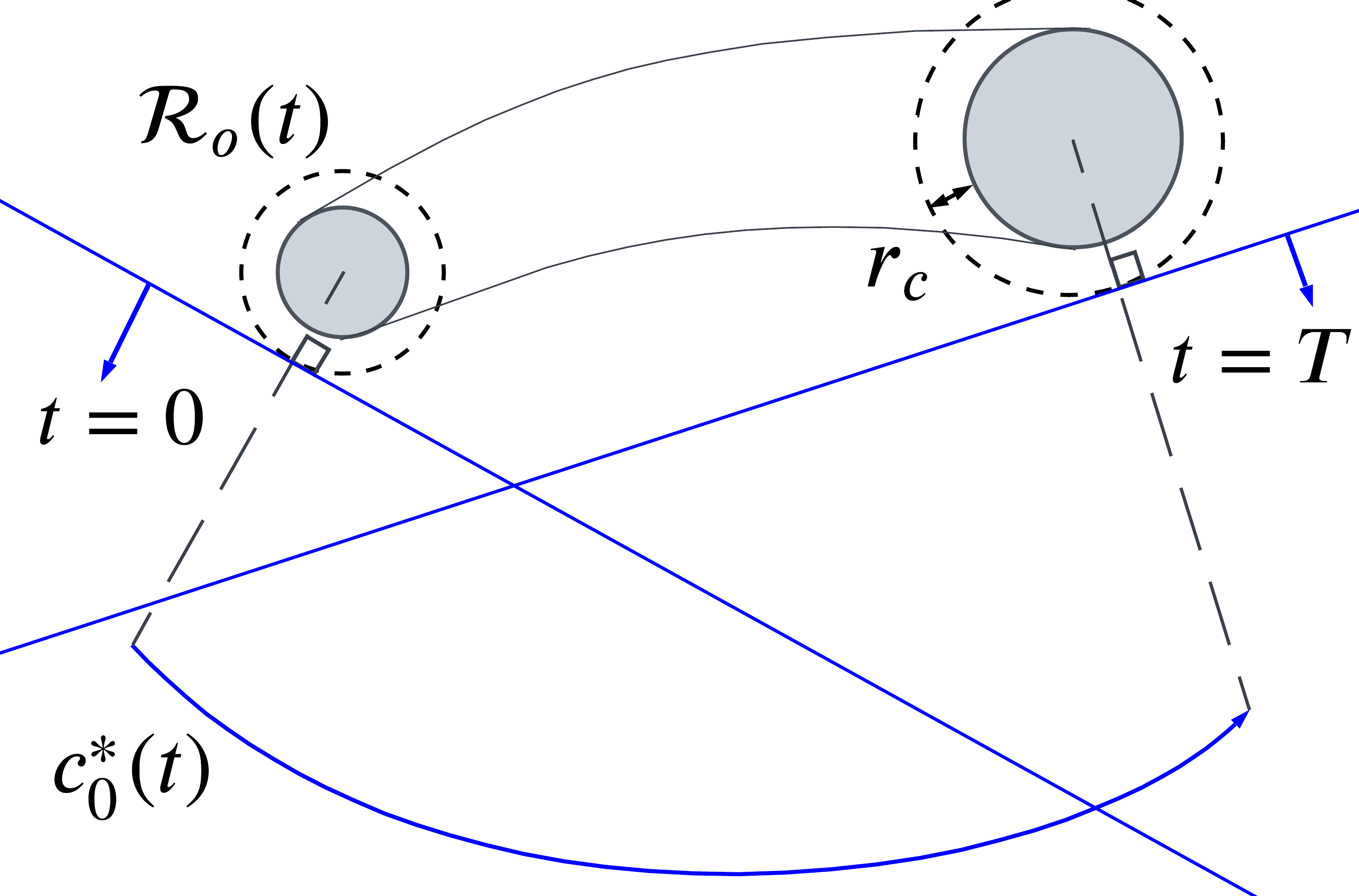
(d)

Figure 5: (a) TVR-O (blue: Class O1, green: Class O2) when the reachable sets of the target (red) and obstacles (grey) are distant from each other. (b) TVR-O (purple) when the reachable sets of the target (red) and obstacles (grey) overlap. (c) TVR-F (blue: Class F1, green: Class F2). (d): Collision-free region (blue) against an obstacle (grey).

VI-B Target Visible Region

To robustly maintain the visibility of the target against prediction error, the target visible region TVR is defined considering the reachable sets of the moving objects: $\mathcal{R}_{\textbf{q}}(t)$ and $\mathcal{R}_{\textbf{o}}(t)$.

VI-B1 Target visibility against obstacles

We define the target visible region against an obstacle (TVR-O), for each obstacle. In order to maximize a visible area of the targets’ reachable set that is not occluded by the reachable set of obstacles, TVR-O is set to a half-space so that it includes $\mathcal{R}_{\textbf{q}}(t)$ and minimizes the area that overlaps with $\mathcal{R}_{\textbf{o}}(t)$.

In the case where the reachable sets of the target and obstacles do not overlap, we define $\mathcal{V}_{O}(t)$ as a half-space made by a tangential line between $\mathcal{R}_{\textbf{q}}(t)$ and $\mathcal{R}_{\textbf{o}}(t)$ as shown in Fig. 5(a), and TVR-O is represented as the following:

$$\mathcal{V}_{O}(t)=\Big{\{}\textbf{x}(t)\in\mathbb{R}^{2}|\ {}_{\hat{\textbf{o}}}\hat{\textbf{q}}^{T}(t)\begin{bmatrix}r_{qo}(t)&\mp d_{2}(t)\\ \pm d_{2}(t)&r_{qo}(t)\end{bmatrix}{}_{\hat{\textbf{o}}}\textbf{x}(t)$$ (18)

$$-r_{o}(t)d_{1}^{2}(t)\geq 0\Big{\}}$$

where $r_{qo}(t)=r_{q}(t)+r_{o}(t)$, $d_{1}(t)=\|{}_{\textbf{o}}\hat{\textbf{q}}(t)\|_{2}$, and $d_{2}(t)=(d_{1}^{2}(t)-r_{qo}^{2}(t))^{\frac{1}{2}}$. The double signs in (18) are in the same order, where the lower and upper signs are for Class O1 and Class O2, respectively.

Lemma 1.

If $\textbf{c}(t)\in\mathcal{V}_{O}(t)$, $L(\textbf{c}(t),\mathcal{R}_{q}(t))\subset\mathcal{F}\setminus\mathcal{R}_{\textbf{o}}(t)$ is satisfied.

Proof.

$\mathcal{V}_{O}(t)$ is a half-space which is convex, and both $\textbf{c}(t)$ and $\mathcal{R}_{\textbf{q}}(t)$ belongs to $\mathcal{V}_{O}(t)$. By the definition of convexity, all Line-of-Sight connecting the drone $\textbf{c}(t)$ and all points in the reachable set of the target $\mathcal{R}_{\textbf{q}}(t)$ are included in $\mathcal{V}_{O}(t)$. Since the TVR-O defined in (18) are disjoint with $\mathcal{R}_{\textbf{o}}(t)$, $L(\textbf{c}(t),\mathcal{R}_{q}(t))\subset\mathcal{F}\setminus\mathcal{R}_{\textbf{o}}(t)$. ∎

Remark 1.

In dual-target scenarios, in order to avoid the occlusion of a target by another target, (18) is further defined by considering one of the targets as an obstacle.

For the case where the reachable sets overlap, TVR-O becomes a half-space made by a tangential line to the $\mathcal{R}_{o}(t)$ which is perpendicular to a line segment connecting centers of the target $\hat{\textbf{q}}(t)$ and the obstacles $\hat{\textbf{o}}(t)$, illustrated as straight lines in Fig. 5(b). Then the TVR-O is represented as

$$\mathcal{V}_{O}(t)=\{\textbf{x}(t)\in\mathbb{R}^{2}|{}_{\hat{\textbf{o}}}\hat{\textbf{q}}^{T}(t){}_{\hat{\textbf{q}}}\textbf{x}(t)-r_{q}(t)d_{1}(t)\geq 0\}$$ (19)

All terms in (18)-(19) are polynomials except $d_{1}(t)$ and $d_{2}(t)$. We convert $d_{1}(t),d_{2}(t)$ into Bernstein polynomials with a numerical technique that origins from Lagrange interpolation with standard polynomial representation [28].
For the time interval $[T_{m},T_{m+1}]$, $d_{i}(t),i=1,2$ are approximately represented as $\tilde{d}_{i}(t)=\sum_{j=0}^{\tilde{n}_{i}}\tilde{d}_{i,m,j}B_{j,\tilde{n}_{i}}(t,T_{m},T_{m+1})$. $\tilde{n}_{i}$ is the degree of $\tilde{d}_{i}(t)$, and control points $\tilde{\textbf{d}}_{i}=[\tilde{d}_{i,m,0},\ldots,\tilde{d}_{i,m,\tilde{n}_{i}}]^{T}$ can be acquired as follows:

$$\tilde{\textbf{d}}_{i}=B_{\tilde{n}_{i}}^{-1}\textbf{d}_{i}^{\prime}$$ (20)

where $B_{\tilde{n}_{i}}=\{b_{j,k}\}\in\mathbb{R}^{(\tilde{n}_{i}+1)\times(\tilde{n}_{i}+1)}$ is a Bernstein-Vandermonde matrix [29] with elements given by $b_{j,k}=\begin{pmatrix}\tilde{n}_{i}\\ k\end{pmatrix}$ ${\Big{(}\dfrac{j}{\tilde{n}_{i}}\Big{)}}^{k}{\Big{(}\dfrac{\tilde{n}_{i}-j}{\tilde{n}_{i}}\Big{)}}^{\tilde{n}_{i}-k},\ j,k=0,\ldots,\tilde{n}_{i}$, and $\textbf{d}_{i}^{\prime}\in\mathbb{R}^{\tilde{n}_{i}+1}$ consists of $\tilde{n}_{i}+1$ sequential samples $d_{i}\big{(}(1-\frac{l}{\tilde{n}_{i}})T_{m}+\frac{l}{\tilde{n}_{i}}T_{m+1}\big{)},\ l=0,\ldots,\tilde{n}_{i}$.
With the approximated terms $\tilde{d}_{1}(t),\tilde{d}_{2}(t)$, we represent the target visibility constraint as the following:

$$\text{Case 1}:\ t\in[T_{i},T_{i+1}],\ \text{s.t. }\mathcal{R}_{q}(t)\cap\mathcal{R}_{o}(t)=\emptyset:$$ (21a)

$$\quad\quad{}_{\hat{\textbf{o}}}\hat{\textbf{q}}^{T}(t)\begin{bmatrix}r_{qo}(t)&\mp\tilde{d}_{2}(t)\\ \pm\tilde{d}_{2}(t)&r_{qo}(t)\end{bmatrix}{}_{\hat{\textbf{o}}}\textbf{c}(t)-r_{o}(t){d}_{1}^{2}(t)\geq 0$$

$$\text{Case 2}:\ t\in[T_{i},T_{i+1}],\ \text{s.t. }\mathcal{R}_{q}(t)\cap\mathcal{R}_{o}(t)\neq\emptyset:$$ (21b)

$$\quad\quad{}_{\hat{\textbf{o}}}\hat{\textbf{q}}^{T}(t){}_{\hat{\textbf{q}}}\textbf{c}(t)-r_{q}(t)\tilde{d}_{1}(t)\geq 0$$

VI-B2 FOV constraints

In addition to (21), FOV limit should be considered in the case where the drone follows dual-target. Circles, whose inscribed angle of an arc tracing points $Q_{1}$ and $Q_{2}$ at $\hat{\textbf{q}}_{1}(t)$, $\hat{\textbf{q}}_{2}(t)$ equals to $\theta_{f}$, are uniquely defined and represented as follows.

$$\mathcal{D}_{i}(t)=\mathcal{B}(\textbf{f}_{i}(t),r_{f}(t)),\ i=1,2\ ,$$ (22)

$$\textbf{f}_{i}(t)=\frac{1}{2}\begin{bmatrix}1&(-1)^{i+1}\cot{\theta_{f}}\\ (-1)^{i}\cot{\theta_{f}}&1\end{bmatrix}{}_{\hat{\textbf{q}}_{1}}\hat{\textbf{q}}_{2}(t)+\hat{\textbf{q}}_{1}(t),$$

$$r_{f}(t)=\frac{1}{2\sin{\theta_{f}}}\|{}_{\hat{\textbf{q}}_{1}}\hat{\textbf{q}}_{2}(t)\|_{2},\ {}_{\hat{\textbf{q}}_{1}}\hat{\textbf{q}}_{2}(t)=\hat{\textbf{q}}_{2}(t)-\hat{\textbf{q}}_{1}(t)$$

According to a geometric property of an inscribed angle, $\angle Q_{1}XQ_{2}>\theta_{f}$, $\angle Q_{1}YQ_{2}<\theta_{f}$ for $\forall X\in\mathcal{D}_{z}(t)\setminus\partial\mathcal{D}_{z}(t)$, $\forall Y\notin\mathcal{D}_{z}(t)$, where $D_{z}(t)$ is represented as follows.

$$\mathcal{D}_{z}(t)=\begin{cases}&\mathcal{D}_{1}(t)\cap\mathcal{D}_{2}(t)\quad(\text{if}\ \theta_{f}\geq\frac{\pi}{2})\\ &\mathcal{D}_{1}(t)\cup\mathcal{D}_{2}(t)\quad(\text{if}\ \theta_{f}<\frac{\pi}{2})\end{cases}$$ (23)

Since the camera FOV is $\theta_{f}$, the drone inside $D_{z}(t)$ misses at least one target in the camera image inevitably, and the drone outside of $\mathcal{D}_{z}(t)$ is able to see both targets.

We define the target visible region considering camera FOV (TVR-F) as a half-space that does not include $\mathcal{D}_{z}(t)$ and is tangential to $\mathcal{D}_{z}(t)$ as shown in Fig. 5(c). It is represented as follows.

$$\mathcal{V}_{F}(t)=\{\textbf{x}(t)|\pm\text{det}(\begin{bmatrix}{}_{\hat{\textbf{q}}_{1}}\textbf{x}^{T}(t)\\ {}_{\hat{\textbf{q}}_{1}}\hat{\textbf{q}}_{2}^{T}(t)\end{bmatrix}-\frac{1+\cos{\theta_{f}}}{2\sin{\theta_{f}}}\|{}_{\hat{\textbf{q}}_{1}}\hat{\textbf{q}}_{2}(t)\|_{2}^{2}\geq 0\}$$ (24)

Upper and lower signs are for Class F1 and Class F2, respectively, where the class is defined as

$$\begin{cases}&\textit{Class F1}\ (\text{if}\ \det\begin{bmatrix}{}_{\hat{\textbf{q}}_{1}}\textbf{c}^{T}(0)\\ {}_{\hat{\textbf{q}}_{1}}\hat{\textbf{q}}_{2}^{T}(0)\end{bmatrix}\geq 0)\\ &\textit{Class F2}\ (\text{if}\ \det\begin{bmatrix}{}_{\hat{\textbf{q}}_{1}}\textbf{c}^{T}(0)\\ {}_{\hat{\textbf{q}}_{1}}\hat{\textbf{q}}_{2}^{T}(0)\end{bmatrix}<0)\\ \end{cases}$$ (25)

We make the drone satisfy $\textbf{c}(t)\in\mathcal{V}_{F}(t)$ to see the both targets.

VI-C Collision Avoidance

To avoid collision with obstacles, we define a collision-free area as a half-space made by a tangential line to a set inflated by $r_{c}$ from $\mathcal{R}_{o}(t)$ considering $\textbf{c}_{0}^{*}(t)$, a planning result in the previous step. It is shown in Fig.5(d) and can be represented as the following.

$$\mathcal{F}_{c}(t)=\{\textbf{x}(t)\in\mathbb{R}^{2}|{}_{\hat{\textbf{o}}}\textbf{c}_{0}^{*T}(t){}_{\hat{\textbf{o}}}\textbf{x}(t)\geq(r_{o}(t)+r_{c})\|{}_{\hat{\textbf{o}}}\textbf{c}_{0}^{*}(t)\|_{2}\}$$ (26)

${}_{\hat{\textbf{o}}}\textbf{c}_{0}^{*}(t):=\textbf{c}_{0}^{*}(t)-\hat{\textbf{o}}(t)$. As in (20), we approximate a non-polynomial term $\|{}_{\hat{\textbf{o}}}\textbf{c}_{0}^{*}(t)\|_{2}$ to a polynomial $\tilde{d}_{3}(t)$. With the approximated the term $\tilde{d}_{3}(t)$, the collision constraint is defined as follows:

$${}_{\hat{\textbf{o}}}\textbf{c}_{0}^{*T}(t){}_{\hat{\textbf{o}}}\textbf{c}(t)-(r_{o}(t)+r_{c})\tilde{d}_{3}(t)\geq 0$$ (27)

Due to the fact that the multiplication of Bernstein polynomials is also a Bernstein polynomial, the left-hand side of the (21), (24), (27) can be represented in a Bernstein polynomial form. With the non-negativeness property of Bernstein basis, we make coefficients of each basis non-negative in order to keep the left-hand side non-negative, and (21), (24), (27) turn into affine constraints with the decision vector $\underline{\textbf{c}}$. The constraints can be written as follows, and we omit details.

$$A_{\text{TVR-O}}\underline{\textbf{c}} \geq\textbf{b}_{\text{TVR-O}},$$ (28)

$$A_{\text{TVR-F}}\underline{\textbf{c}} \geq\textbf{b}_{\text{TVR-F}},$$

$$A_{\text{Colli}}\underline{\textbf{c}} \geq\textbf{b}_{\text{Colli}}$$

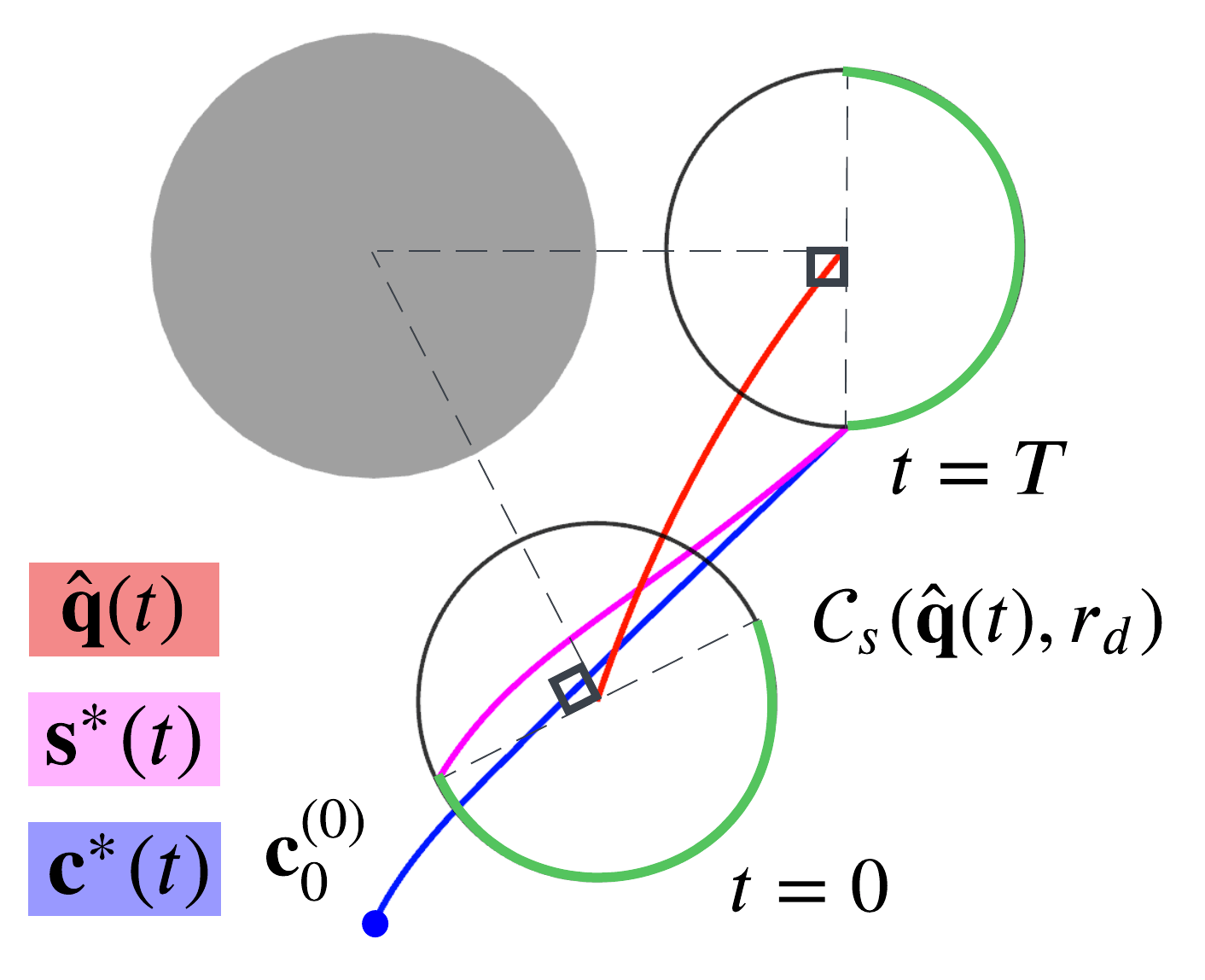
(a)

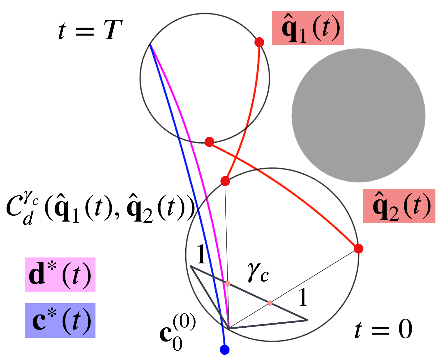
(b)

Figure 6: Reference trajectory design in single- and dual-target (red) among obstacles (grey). (a): The points having the maximum visibility score $\psi$ in $\mathcal{C}_{s}(\hat{\textbf{q}}(t),r_{d})$ (green), a trajectory with the maximum $\psi$, $\textbf{s}^{*}(t)$ (magenta), and the reference trajectory $\textbf{c}^{*}(t)$ (blue line) considering current position of the drone (blue dot). (b): $\mathcal{C}_{d}^{\gamma_{c}}(\hat{\textbf{q}}_{1}(t),\hat{\textbf{q}}_{2}(t))$ (black circle). The trajectory with high $\psi$, $\textbf{d}^{*}(t)$ (magenta), and the reference trajectory $\textbf{c}^{*}(t)$ (blue line) considering current position of the drone (blue dot).

VI-D Reference Trajectory for Target Tracking

In this section, we propose a reference trajectory for target chasing that enhances the visibility of the targets.

VI-D1 Single target

Referring to [12], the visibility score is taken using Euclidean Distance Field (EDF) $\phi(\cdot)$ [30] in designing the reference trajectory. Definition of the visibility score is the closest distance between all points in an $i$-th obstacle, $\mathcal{O}_{i}$, and the Line-of-Sight connecting the target and the drone, and it is represented as

$$\psi(\textbf{c}(t);\hat{\textbf{q}}(t),\mathcal{O}_{i})=\min_{L(\textbf{c}(t),\hat{\textbf{q}}(t))}\phi(\textbf{c}(t),\mathcal{O}_{i})$$ (29)

In order to keep the dimension of the target, that is projected to the camera image, we set the desired shooting distance $r_{d}$. With the desired shooting distance $r_{d}$, a viewpoint candidate set can be defined as $\mathcal{C}_{s}(\hat{\textbf{q}}(t),r_{d})$ $=\partial\mathcal{B}(\hat{\textbf{q}}(t),r_{d})$. Under the assumption that the environment consists of cylindrical obstacles, half-circumference of $\mathcal{C}_{s}(\hat{\textbf{q}}(t),r_{d})$ acquires the maximum visibility score as illustrated in green in Fig. 6(a). Therefore, the following trajectory maintains the maximum $\psi$ against the $\mathcal{O}_{i}$.

$$\textbf{s}_{i}(t)=\textbf{q}(t)+r_{d}[\cos{\delta_{i}(t)},\sin{\delta_{i}(t)}]^{T}$$ (30)

where $\delta_{i}(t)=\tan^{-1}({}_{\hat{\textbf{o}}_{i}}\hat{\textbf{q}}_{y}(t))/{}_{\hat{\textbf{o}}_{i}}\hat{\textbf{q}}_{x}(t))\mp\frac{\pi}{2}$. The upper and lower signs are for Class O1 and Class O2, respectively. We define the reference trajectory as a weighted sum of $\textbf{s}_{i}(t)$.

$$\textbf{s}^{*}(t)=\Big{(}\sum_{i=1}^{N_{o}}w_{i}\Big{)}^{-1}\sum_{i=1}^{N_{o}}w_{i}\textbf{s}_{i}(t)$$ (31)

$w_{i}$s are weight functions that are inverse proportion to the current distance between the target and each obstacle.

VI-D2 Dual target

In order to make aesthetically pleasing scenes, we place two targets in a ratio of $1:\gamma_{c}:1$ on the camera image. To do so, the drone must exist in a set $\mathcal{C}_{d}^{\gamma_{c}}(\hat{\textbf{q}}_{1}(t),\hat{\textbf{q}}_{2}(t))$, which is defined as follows and is illustrated as a black circle in Fig. 6(b).

$$\mathcal{C}_{d}^{\gamma_{c}}(\hat{\textbf{q}}_{1}(t),\hat{\textbf{q}}_{2}(t))=\partial\mathcal{B}(\textbf{f}_{c}(t),r_{f,c}(t)),$$ (32)

$$\textbf{f}_{c}(t)=\frac{1}{2}(\hat{\textbf{q}}_{1}(t)+\hat{\textbf{q}}_{2}(t))\pm$$

$$\quad\frac{\gamma_{c}+2}{4\gamma_{c}}\cot{\frac{\theta_{f}}{2}}\Big{(}1-\frac{\gamma_{c}^{2}}{(\gamma_{c}+2)^{2}}\tan^{2}{\frac{\theta_{f}}{2}}\Big{)}\begin{bmatrix}0&1\\ -1&0\end{bmatrix}{}_{\hat{\textbf{q}}_{1}}\hat{\textbf{q}}_{2}(t),$$

$$r_{f,c}(t)=\frac{\gamma_{c}+2}{4\gamma_{c}}\cot{\frac{\theta_{f}}{2}}\Big{(}1+\frac{\gamma_{c}^{2}}{(\gamma_{c}+2)^{2}}\tan^{2}{\frac{\theta_{f}}{2}}\Big{)}\|{}_{\hat{\textbf{q}}_{1}}\hat{\textbf{q}}_{2}(t)\|_{2}$$

where the upper and lower signs are for Class F1 and Class F2. We define the reference trajectory to acquire high visibility score $\psi$ while maintaining the ratio.

$$\textbf{d}^{*}(t)=\textbf{f}_{c}(t)+r_{f,c}(t)[\cos{\delta_{d}}(t),\sin{\delta_{d}(t)}]^{T},$$ (33)

$$\delta_{d}(t)=\tan^{-1}{\frac{\sum_{i=1}^{2N_{o}}w_{i}\sin{\delta_{i}(t)}+w_{m}\sin{\delta_{m}(t)}}{\sum_{i=1}^{2N_{o}}w_{i}\cos{\delta_{i}(t)}+w_{m}\cos{\delta_{m}(t)}}}$$

where $\delta_{m}(t)=\tan^{-1}({}_{\hat{\textbf{q}}_{1}}\hat{\textbf{q}}_{2y}(t))/{}_{\hat{\textbf{q}}_{1}}\hat{\textbf{q}}_{2x}(t))\mp\frac{\pi}{2}$, and $w_{i}$ and $\delta_{i}(t)$ are defined as in (30), for two targets. The upper and lower signs are for Class F1 and Class F2, respectively. $\delta_{m}(t)$ is defined as the furthest direction from the two targets to maximize a metric, $\psi(\textbf{c}(t);\hat{\textbf{q}}_{1}(t),\hat{\textbf{q}}_{2}(t))$ + $\psi(\textbf{c}(t);\hat{\textbf{q}}_{2}(t),\hat{\textbf{q}}_{1}(t))$, which can represent the visibility score between two targets. For numerical stability in the QP solver, the reference trajectory is redefined by the interpolation between $\boldsymbol{\mu}^{*}(t)$, $\boldsymbol{\mu}=\textbf{s},\textbf{d}$ and the current position of the drone $\textbf{c}^{(0)}_{0}$. With a non-decreasing polynomial function $\alpha(t)$ such that $\alpha(0)=0$, $\alpha(T)=1$, the reference trajectory is defined as follows.

$$\textbf{c}^{*}(t)=\big{(}1-\alpha(t)\big{)}\textbf{c}^{(0)}_{0}+\alpha(t)\boldsymbol{\mu}^{*}(t)$$ (34)

Since trigonometric terms in (31),(33) are non-polynomial, the Lagrange interpolation is used as (20). The approximated $\textbf{c}^{*}(t)$ is denoted as $\tilde{\textbf{c}}^{*}(t)$. Based on the construction of reference trajectory and target visibility constraints, we formulate the trajectory optimization problem as a QP problem.

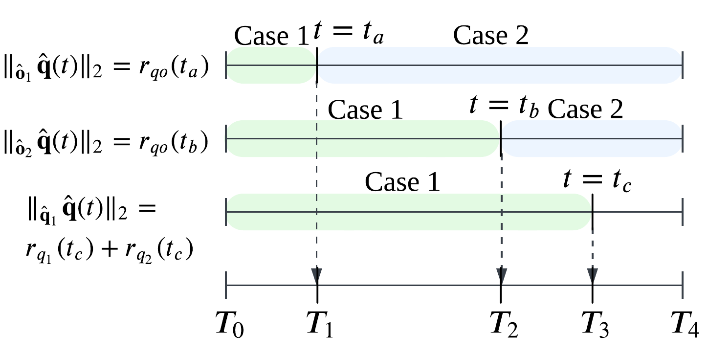
Figure 7: Time segmentation. Green and blue regions are time intervals when the (21a) and (21b) are adopted as visibility constraints, respectively.

VI-E QP Formulation

VI-E1 Trajectory segmentation

The constraint (21) is divided into the cases, when the reachable sets are separated and when they overlap. To apply (21) according to the situation, the roots of equations $\|{}_{\hat{\textbf{o}}}\hat{\textbf{q}}(t)\|_{2}=r_{qo}(t)$ and $\|{}_{\hat{\textbf{q}}_{1}}\hat{\textbf{q}}_{2}(t)\|_{2}=r_{q1}(t)+r_{q2}(t)$. should be investigated for $t\in(0,T)$. $[T_{0},\ldots,T_{M}]$ is defined through root finding, and we set $M$ polynomial segments to optimize, as stated in (5). Fig. 7 visualizes the above process.
Due to the virtue of De Casteljau’s algorithm [31], the single Bernstein polynomial such as $\hat{\textbf{q}}(t),r_{q}(t)$ can be divided into $M$ Bernstein polynomials. With the information with $M$-segment-polynomial representation, we formulate a QP problem.

TABLE III: Computation time in QP solver

	Computation		$n_{c}=4$					$n_{c}=5$					$n_{c}=6$
	time [ms]		# polynomial segment $(M)$					# polynomial segment $(M)$					# polynomial segment $(M)$
			1	2	3	4	5	1	2	3	4	5	1	2	3	4	5
Single	# obstacle	1	$0.17$	$0.54$	$\cdot$	$\cdot$	$\cdot$	$0.19$	$0.77$	$\cdot$	$\cdot$	$\cdot$	$0.21$	$1.16$	$\cdot$	$\cdot$	$\cdot$
	$(N_{o})$	2	$0.18$	$0.71$	$2.07$	$\cdot$	$\cdot$	$0.22$	$1.12$	$2.95$	$\cdot$	$\cdot$	$0.24$	$1.66$	$4.45$	$\cdot$	$\cdot$
		3	$0.29$	$0.98$	$2.91$	$6.05$	$\cdot$	$0.34$	$1.23$	$4.58$	$8.05$	$\cdot$	$0.43$	$1.82$	$5.62$	$12.3$	$\cdot$
		4	$0.32$	$1.01$	$2.75$	$7.81$	$12.2$	$0.39$	$1.38$	$4.24$	$12.6$	$18.8$	$0.55$	$1.88$	$6.81$	$16.8$	$24.8$
Dual	# obstacle	1	$0.18$	$0.66$	$1.94$	$5.34$	$\cdot$	$0.20$	$0.91$	$2.95$	$7.61$	$\cdot$	$0.26$	$1.38$	$4.46$	$10.5$	$\cdot$
	$(N_{o})$	2	$0.21$	$1.21$	$3.94$	$5.82$	$13.6$	$0.46$	$1.72$	$6.78$	$9.48$	$21.4$	$0.55$	$2.41$	$10.8$	$17.8$	$36.3$
		3	$0.43$	$1.67$	$3.86$	$8.54$	$17.8$	$0.78$	$2.51$	$5.62$	$13.5$	$28.6$	$0.81$	$3.72$	$8.91$	$21.8$	$43.6$

VI-E2 Constraints

We set up affine constraints with respect to $\underline{\textbf{c}}$ to keep dynamic feasibility and the visibility of the target and avoid collision. Dynamic constraints consist of constraints regarding an initial state, limits of velocity and acceleration, and continuity between consecutive polynomial segments. For the details, see Appendix C-A. Then, for the visibility of the target and the safety of the drone, the constraints in (28) are applied.

VI-E3 Costs

We minimized jerky motion and reference tracking errors.

$$J=\int_{0}^{T}\|\textbf{c}^{(3)}(t)\|_{2}^{2}+w_{e}\|\textbf{c}(t)-\tilde{\textbf{c}}^{*}(t)\|_{2}^{2}dt$$ (35)

$w_{e}$ is a weight factor of tracking cost. The designed cost is quadratic with the decision vector $\underline{\textbf{c}}$. For the details, see Appendix. C-B.

Since all the constraints are affine, and the cost is quadratic with respect to $\underline{\textbf{c}}$, the Chasing Problem (3) is reformulated as a QP problem.

$$\underset{\underline{\textbf{c}}}{\text{min}} \underline{\textbf{c}}^{T}Q_{c}\underline{\textbf{c}}+\textbf{g}_{c}^{T}\underline{\textbf{c}}$$ (36)

s.t. $$A_{c}\underline{\textbf{c}}\geq\textbf{b}_{c}$$

VI-F Evaluation

We set $n_{c}$ as 4, 5, 6 and test 5000 times for different scenarios $N_{o}$ $=1,2,3,4$. qpOASES [32] is utilized as a QP solver, and the execution time to solve a QP problem is summarized in Table. III. As you can see in the table, the computation time increases as the number of segments and obstacles increases. To satisfy real-time criteria (10Hz), as $N_{o}$ increases, we reduce $r_{q}(t)$ by defining $\epsilon_{p}|\mathcal{P}_{s}|$ furthest primitives as outliers and removing them from $\mathcal{P}_{s}$ and recalculate $\mathcal{R}_{\textbf{q}}(t)$. It is visualized in Fig. 4(c) and can lower the number of segments $M$. With this strategy, real-time planning is possible even in complex and dense environments.

VII Chasing Scenario Validation

VII-A Implementation Details

We perform AirSim [33] simulation for a benchmark test of our method and [20], [24]. In real-world experiments, stereo cameras ZED2 [34] are mounted on the drone, and intel NUC and Jetson Xavier NX are equipped as onboard computers. As a flight controller, Pixhawk4 is used. In addition to the odometry function in the camera, we utilize 3D human pose estimation, and humans are distinguished by color as in [24]. An algorithm in [35] is used to build a static obstacle map.

In scenarios involving multiple moving objects, visual odometry suffers from dynamic objects in a camera image. We install two ZED2 cameras facing the opposite direction. The front-view sensor is for object detection and tracking, and the rear-view one is for the localization of the robot. Since the rear-view sensor does not contain multiple moving objects in the camera image, the localization system is free from visual interference by dynamic objects, which can prevent degradation of localization performance.

In both simulations and experiments, two actors move in environments: one is a target and the other is considered a dynamic obstacle (interrupter) in single-target scenarios whereas two actors are both targets in dual-target scenarios. For consistent acquisition of positional and scale data of the target and the interrupter, the drone looks between them. Besides, the drone adjusts its altitude to the height of the target. The parameters used in validations are summarized in Table. IV.

TABLE IV: Problem Settings

Scenario Settings
Name	Single Target	Dual Target
drone radius ($r_{c}$) [m]	0.4	0.4
camera FOV $(\theta_{f})$ $[{}^{\circ}]$	120	120
Prediction Parameters
Name	Single Target	Dual Target
time horizon ($T$) [s]	1.5	1.5
$\#$ sampled points ($N_{samp}$)	1000	1000
Planning Parameters
Name	Single Target	Dual Target
polynomial degree $(n_{c})$	6	6
max velocity ($v_{\text{max}}$) [m/s]	4.0	4.0
max acceleration ($a_{\text{max}}$) [$\text{m}/\text{s}^{2}$]	5.0	5.0
shooting distance ($r_{d}$) [m]	$4.0$	$\cdot$
screen ratio ($\gamma_{c}$)	$\cdot$	1.0
tracking weight ($w_{e}$)	10.0	10.0
jerk weight ($w_{j}$)	1.0	1.0

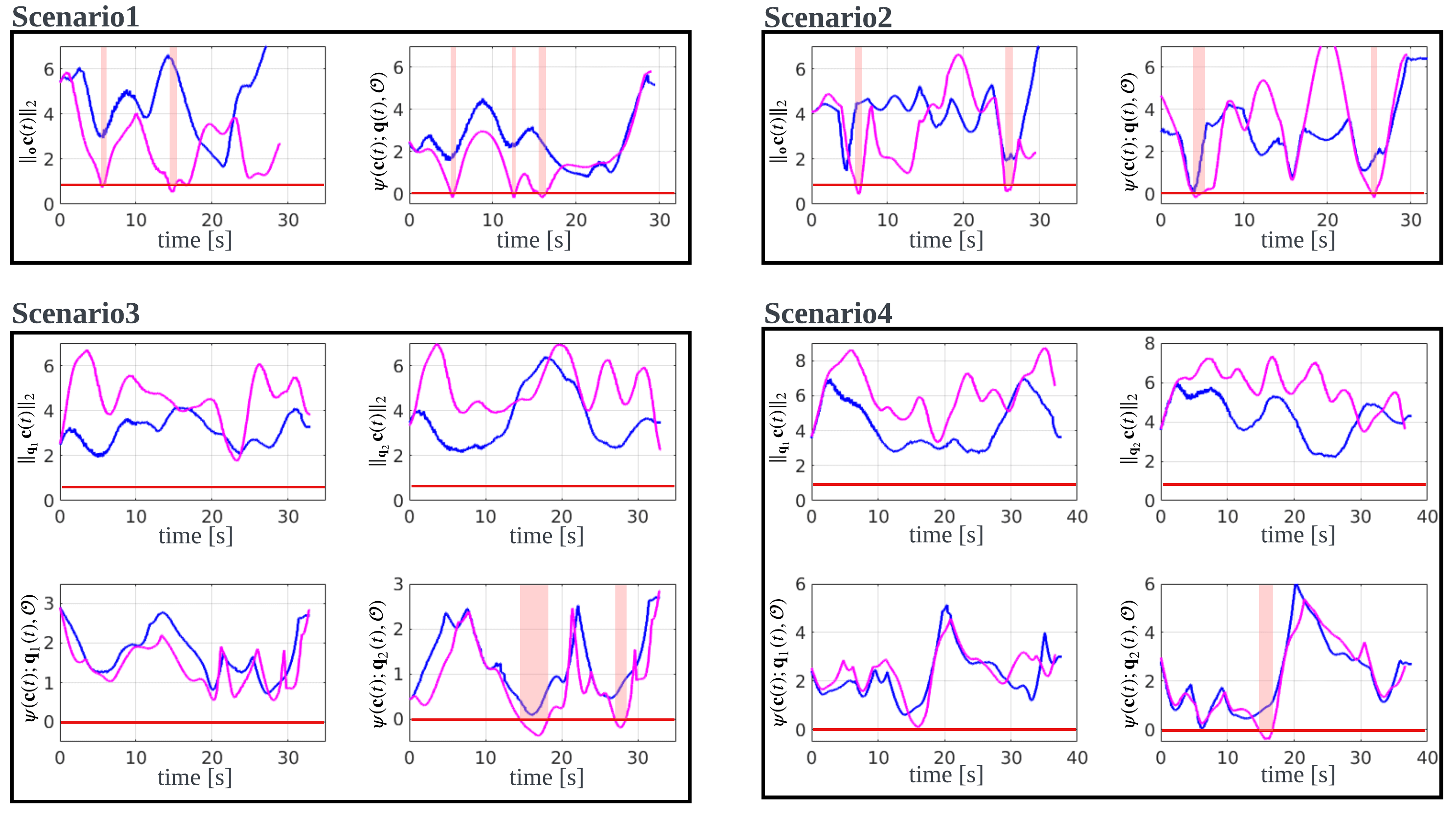
Figure 8: Comparison between the proposed planner (blue) and baselines (magenta) [20],[24]. Scenarios 1-2 and Scenarios 3-4 represent single-target and dual-target scenarios, respectively. In the plots regarding distance, areas below the red lines mean collision, and in the plots regarding visibility score, areas below the red lines mean target occlusion. Red-shaded regions represent the situation when the drone moved by baselines comes into collisions and occlusions.

VII-B Simulations

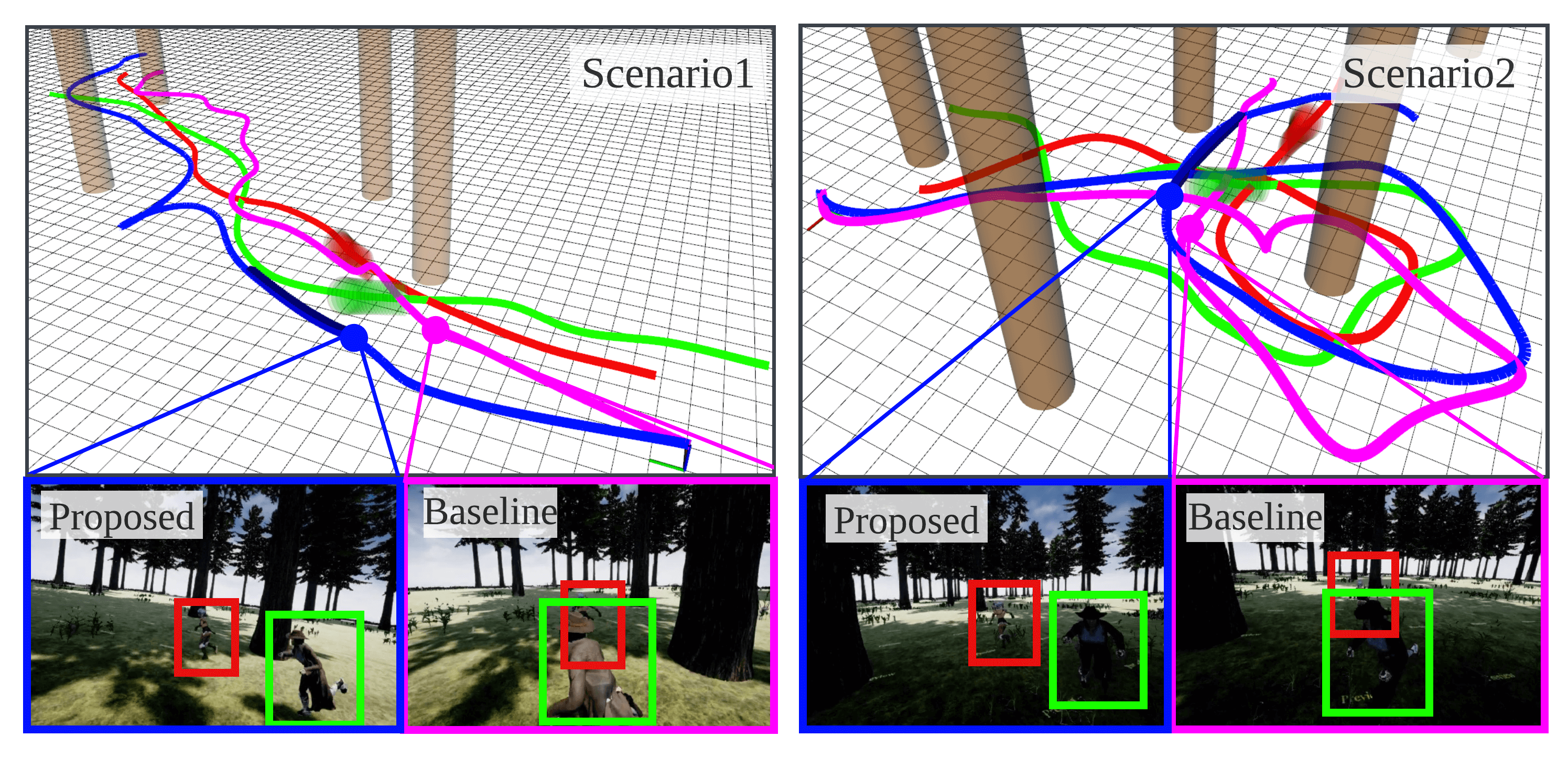
Figure 9: Single-target scenarios. The red and green lines represent the overall paths of the target and the dynamic obstacle respectively. Our planner produces the path for the chasing drone to move along the blue path. The magenta paths are generated by the baseline [20]. The bottom figures are snapshots of the camera images when the interrupter intersects the target’s path and tries to conceal the target’s body.

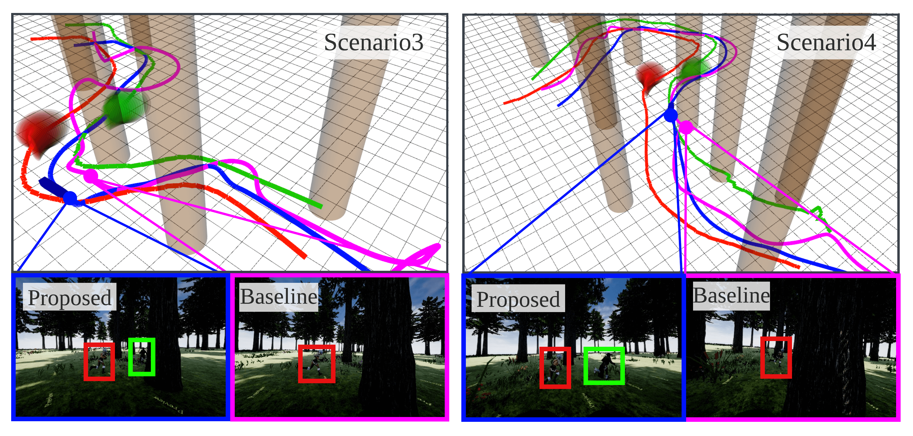
Figure 10: Dual-target scenarios. Two targets move along the red and green paths among obstacles (brown). Snapshots capture the moment when the drone moving by [24] (magenta) misses one of the targets in camera images. Blue paths are generated by our planner and they ensure the drone sees two targets without any occlusion.

We test the proposed planner with four scenarios where two actors run in the forest. The first two scenarios are cases where the first actor is a target, and the other is regarded as an interrupter, while the two remaining scenarios are situations where two actors are both targets. Of the many flight tests, we extract and report 30-40 seconds flights in this paper. In spite of the requirement of heavy computation resources from the physics engine, the planning pipeline is executed within 30 milliseconds.

In the simulation, we compare the proposed planner with the other state-of-the-art planners [20] in single-target chasing scenarios and [24] in dual-target chasing scenarios. We measure the distances between the drone and targets $\|{}_{\textbf{q}}\textbf{c}(t)\|_{2}$, the minimum distance between the drone and obstacles $\|{}_{\textbf{o}}\textbf{c}(t)\|_{2}:=\min(\|{}_{\textbf{o}_{1}}\textbf{c}(t)\|_{2},\ldots,\|{}_{\textbf{o}_{N_{o}}}\textbf{c}(t)\|_{2})$, and a visibility score that is defined as follows:

$$\underset{\mathcal{O}_{i}\in\mathcal{O}}{\min}\psi(\textbf{c}(t);\textbf{q}(t),\mathcal{O}_{i})$$ (37)

As shown in Fig. 8, Fig. 9, and Fig. 10, the proposed approach makes the drone follow the target while maintaining target-visibility safely, whereas collision with obstacles and target-occlusion by the interrupter occur several times when the drone flies by the baseline [20, 24]. Furthermore, in contrast to baselines, the proposed planner adjusts the chasing path so that the drone does not move too far away from the targets. This motion can prevent the degradation of visual object detection and tracking performance.

VII-C Experiments

To validate our chasing strategy, real-world experiments with four and three scenarios are executed for single-target and dual-target tracking, respectively. Two actors move in $8\times 11$ [m²] indoor space with stacked bins. As in the simulations, one actor moves and the other tries to block the target in the drone’s camera view in single-target scenarios, while two actors are both targets in dual-target scenarios.

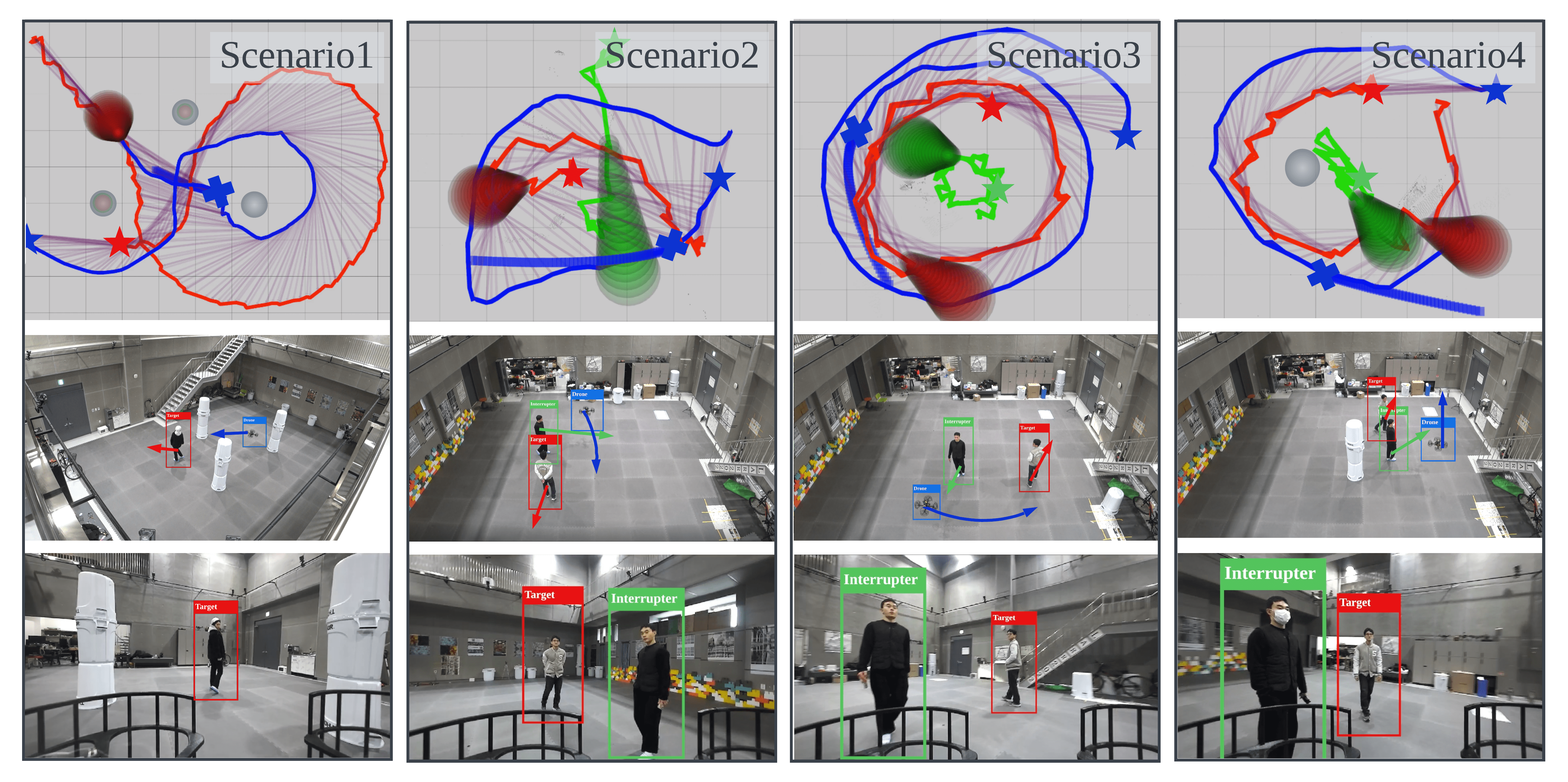
Figure 11: Autonomous aerial tracking in an indoor environment with single-target scenarios. Scenario1: The target (red) moves among white cylindrical obstacles, and the drone (blue) follows the target. Scenario2: The target moves away from the drone, and the interrupter (green) cuts in between the target and the drone. Scenario3: The target moves all over the space, and the interrupter consistently disturbs the target’s tracking. Scenario4: The interrupter intentionally hides behind bins and appears abruptly to obstruct the camera’s view. Stars are the start points of moving objects, blue crosses mean the position of the drone at captured moments, and purple segments represent line-of-sight between the target and the drone.

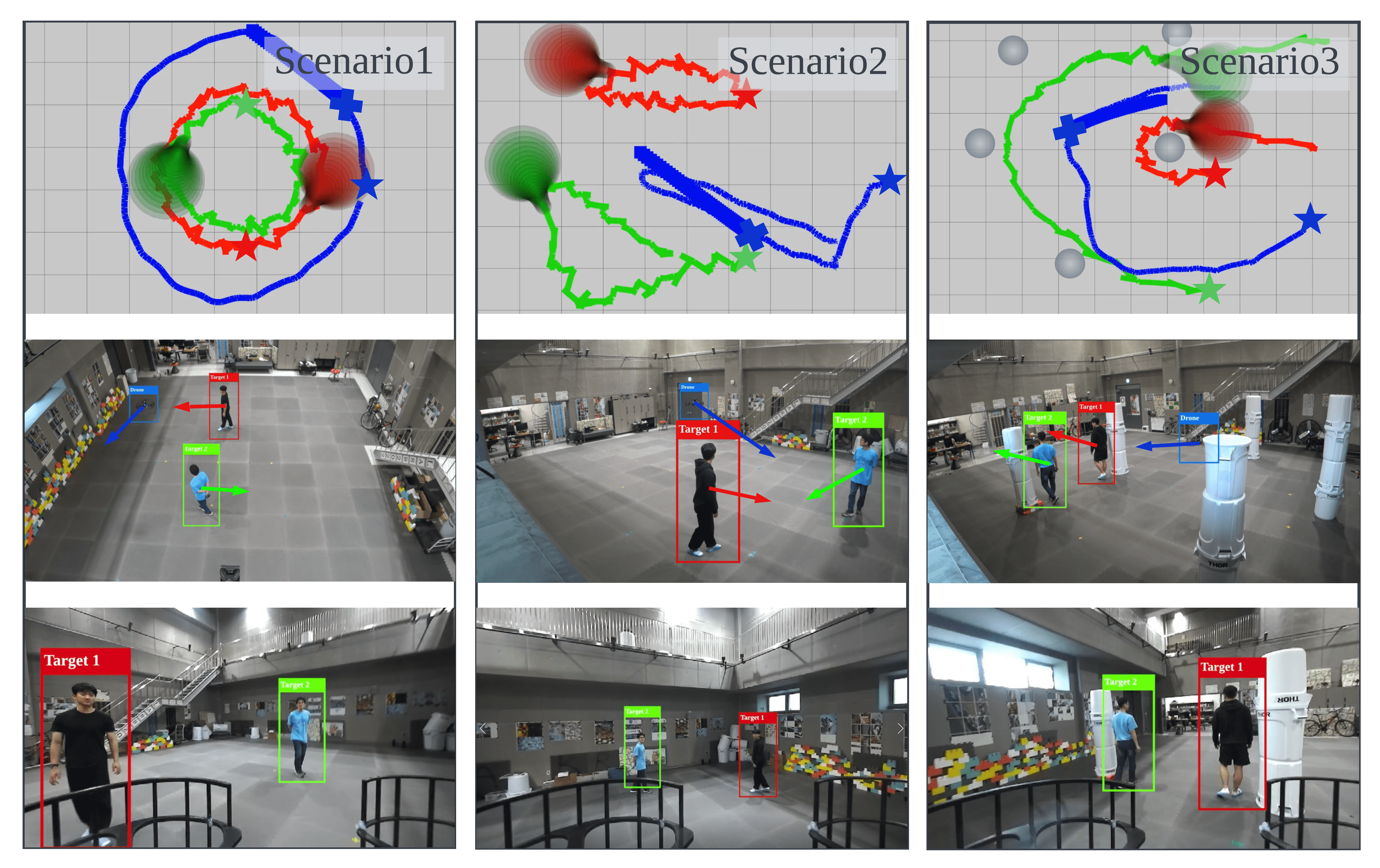
Figure 12: Autonomous aerial tracking in an indoor environment with dual-target scenarios. Scenario1: The targets (red, green) move in a circular motion. Scenario2: The targets move while repeatedly widening and narrowing their relative distance. Scenario3: The targets move among stacked bins (grey). The drone follows targets along blue paths, stars are the start points of moving objects, and blue crosses mean the position of the drone at captured moments.

We update the chasing trajectory at 10Hz, but the actual computation of the entire pipeline takes less than 25 milliseconds. Fig. 11 shows the situations where the drone generates the target-visible path considering the interrupter’s interference and obstacles, and Fig. 12 shows the situations where the drone follows two targets along trajectories considering camera FOV and obstacles. From Fig. 13, we can confirm that the chasing drone’s path is free from collision and occlusion.

To record the camera images in limited computer storage and to transfer images between computers, we use compressed RGB and depth images in the pipeline. Since the compressed data is acquired at a slow rate, information about moving objects is updated slowly; therefore trajectories of moving objects drawn in Fig. 11 and Fig. 12 seem jerky. Nevertheless, the drone succeeds at keeping the visibility of the target and its own safety by quickly updating the chasing trajectory.

VIII Conclusion

We propose a real-time target chasing planner among static and dynamic obstacles. First, we calculate the reachable sets of moving objects in obstacle environments, with Bernstein polynomial primitives. Then, to prevent target occlusion, we define continuous-time target-visible region (TVR) based on the concept of path homotopy, while considering the camera field-of-view limit. The reference trajectory for target tracking is designed and utilized with TVR to formulate trajectory optimization as a single QP problem. The proposed QP formulation can generate dynamically feasible, collision-free, and occlusion-free chasing trajectories in real-time. We extensively demonstrate the effectiveness of the proposed planner through challenging scenaios, including realistic simulations and indoor experiments. In future work, we plan to extend our work to chase multiple targets in dynamic environments.

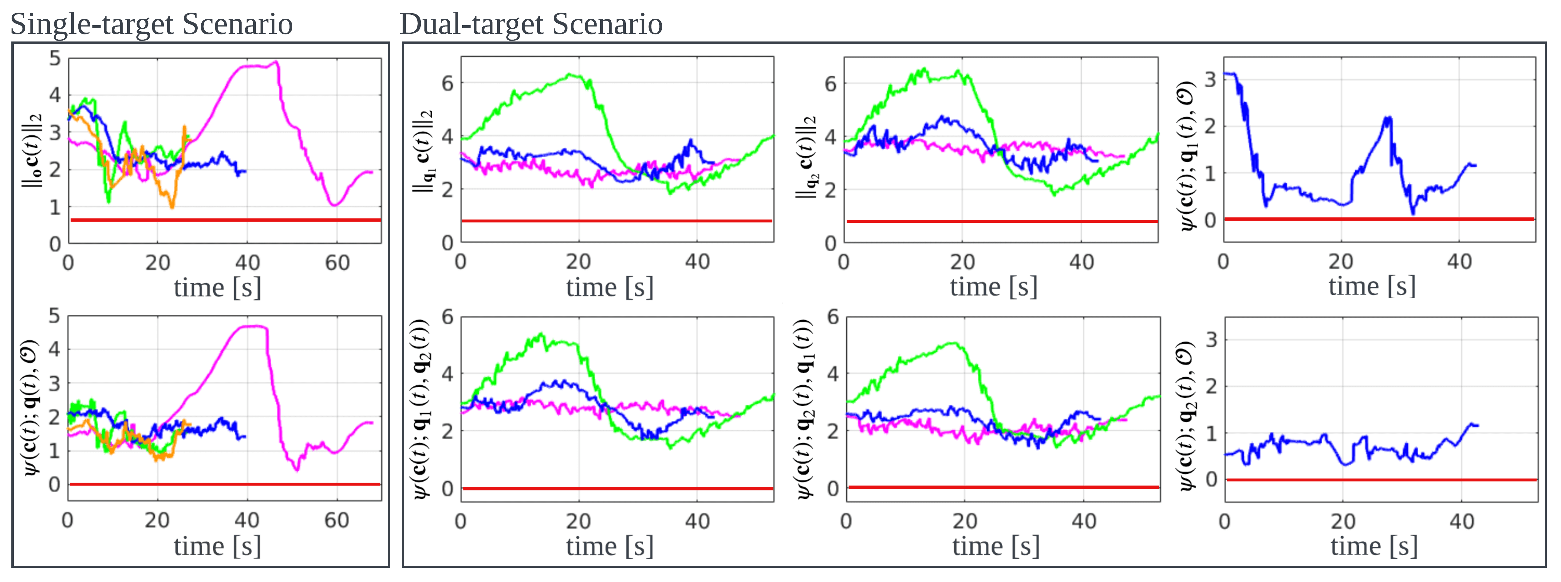
Figure 13: Distance between the drone and objects: obstacles, the targets, and visibility score (29), that are reported in experiments. In the distance plots, areas below the red lines mean collision, and in the visibility score plots, areas below the red lines mean target occlusion. Single-target scenarios {1,2,3,4} match with {magenta, green, blue, orange}, while dual-target scenarios {1,2,3} match with {magenta, green, blue}.

Appendix A Implementation of Collision Check

$$\|\hat{\textbf{p}}_{i}(t)-\textbf{o}_{j}(t)\|_{2}^{2}-(r_{p0}+r_{o_{j}}(t))^{2}\geq 0\Longleftrightarrow$$ (38)

$$\sum_{k=0}^{2n_{p}}\begin{pmatrix}2n_{p}\\ k\end{pmatrix}^{-1}{}^{ij}C_{k}B_{k,2n_{p}}(t,0,T)\geq 0,\ {}^{\forall}j\in\{1,\ldots,|\mathcal{O}|\},$$

where

$${}^{ij}C_{k}\ =\ \ \sum_{l=\max(0,k-n_{p})}^{\min(k,n_{p})}\begin{pmatrix}n_{p}\\ l\end{pmatrix}\begin{pmatrix}n_{p}\\ k-l\end{pmatrix}\Big{(}{}^{ij}_{o}\textbf{p}_{x}[l]\ {}^{ij}_{o}\textbf{p}_{x}[k-l]$$

$$\quad\quad\quad\quad\quad\quad\quad\quad+{}^{ij}_{o}\textbf{p}_{y}[l]\ {}^{ij}_{o}\textbf{p}_{y}[k-l]-{}^{ij}_{o}\textbf{r}[l]\ {}^{ij}_{o}\textbf{r}[k-l]\Big{)},$$

$${}^{ij}_{o}\textbf{p}_{x}=\textbf{p}_{i(x)}-\textbf{o}_{j(x)},\ {}^{ij}_{o}\textbf{p}_{y}=\textbf{p}_{i(y)}-\textbf{o}_{j(y)},\ {}^{ij}_{o}\textbf{r}=\textbf{r}_{o_{j}}+r_{p0}$$

$[l]$ represents $l$-th elements of a vector. The condition ${}^{ij}C_{k}\geq 0,\ k=0,\ldots,2n_{p}$ makes the moving objects do not collide with obstacles during $[0,T]$.

Appendix B Proof of the Proposition1

Motion primitives for object prediction derived from (9) are represented as follows.

$$\hat{\textbf{p}}_{i}(t)=\textbf{P}_{n_{p}}^{T}\textbf{B}_{n_{p}}(t,T)$$ (39)

$$\text{where}\ \textbf{P}_{n_{p}}=E_{3,n_{p}}^{T}\textbf{P}_{3}^{*},$$

$$\textbf{P}_{3}^{*}=[\hat{\textbf{p}}_{0},\hat{\textbf{p}}_{0}+\frac{1}{3}\hat{\textbf{p}}^{(1)}_{0}T,\frac{2}{3}\hat{\textbf{p}}_{0}+\frac{1}{3}\textbf{s}_{p,i}+\frac{1}{3}\hat{\textbf{p}}^{(1)}_{0}T,\textbf{s}_{p,i}]^{T},$$

$$\textbf{B}_{n_{p}}(t,T)=[B_{0,n_{p}}(t,0,T),\ldots,B_{n_{p},n_{p}}(t,0,T)]^{T},\ n_{p}\geq 3,$$

$$E_{m,n}=\{e_{j,k}\}\in\mathbb{R}^{(n+1)\times(m+1)},\ m\geq n,$$

$$e_{j,j+k}=\frac{\begin{pmatrix}n\\ j\end{pmatrix}\begin{pmatrix}m-n\\ k\end{pmatrix}}{\begin{pmatrix}m\\ j+k\end{pmatrix}}$$

The difference between $\hat{\textbf{p}}_{i}(t)$ and $\hat{\textbf{p}}_{j}(t)$, $\|\hat{\textbf{p}}_{i}(t)-\hat{\textbf{p}}_{j}(t)\|=\|\textbf{s}_{p,i}-\textbf{s}_{p,j}\|\frac{t^{2}}{T^{2}}$. Therefore, in order to minimize distance sum in (14), it is sufficient to investigate sampled endpoints.

Appendix C QP Implementation Details

C-A Dynamic Feasibility Constraints

Dynamic constraints in Section VI-E are formulated as follows. First, the trajectory is made to satisfy an initial condition, position and velocity as in (40a),(40b). $\mathcal{C}_{2}$ continuity between consecutive segments is achieved by (40c),(40). Velocity and acceleration are limited by (40),(40).

$$\begin{bmatrix}\textbf{c}_{1(x)}[0]\\ \textbf{c}_{1(y)}[0]\end{bmatrix}=\textbf{c}_{0}^{(0)}$$ (40a)

$$\frac{n_{c}}{(T_{1}-T_{0})}\begin{bmatrix}\textbf{c}_{1(x)}[1]-\textbf{c}_{1(x)}[0]\\ \textbf{c}_{1(y)}[1]-\textbf{c}_{1(y)}[0]\end{bmatrix}=\textbf{c}^{(1)}_{0}$$ (40b)

$$\textbf{c}_{m(\mu)}[n_{c}]=\textbf{c}_{m+1(\mu)}[0],\mu=x,y,\ m=1,\ldots,M-1$$ (40c)

$$\sum_{j=0}^{k}(-1)^{j}\bigg{\{}\frac{\textbf{c}_{m(\mu)}[n_{c}-j]-\textbf{c}_{m(\mu)}[n_{c}-j-1]}{(T_{m}-T_{m-1})^{k+1}}$$

$$-\frac{\textbf{c}_{m+1(\mu)}[j+1]-\textbf{c}_{m+1(\mu)}[j]}{(T_{m+1}-T_{m})^{k+1}}\bigg{\}}=0,$$

$$\mu=x,y,\ k=0,1,\ m=1,\ldots,M-1,$$ (40d)

$$\frac{n_{c}}{T_{m}-T_{m-1}}\big{|}\textbf{c}_{m(\mu)}[j+1]-\textbf{c}_{m(\mu)}[j]\big{|}\leq\frac{1}{\sqrt{2}}v_{\text{max}},$$

$$\mu=x,y,\ m=1,\ldots,M,\ j=0,\ldots,n_{c}-1$$ (40e)

$$\frac{n_{c}(n_{c}-1)}{(T_{m}-T_{m-1})^{2}}\big{|}\textbf{c}_{m(\mu)}[j+2]-2\textbf{c}_{m(\mu)}[j+1]+\textbf{c}_{m(\mu)}[j]\big{|}$$

$$\leq\frac{1}{\sqrt{2}}a_{\text{max}},\ \ \mu=x,y,\ m=1,\ldots,M,\ j=0,\ldots,n_{c}-2$$ (40f)

C-B Costs

The cost (35) is represented as follows:

$$J=\underline{\textbf{c}}^{T}Q\underline{\textbf{c}}+H\underline{\textbf{c}},$$

$$\text{where}\ Q=\begin{bmatrix}Q_{1}&&\boldsymbol{0}\\ &\ddots&\\ \boldsymbol{0}&&Q_{M}\end{bmatrix},H=[H_{1},\ldots,H_{M}],$$ (41a)

$$Q_{i}=w_{j}D_{jerk,i}^{T}B_{jerk,i}^{\int}D_{jerk,i}+w_{e}B_{track,i}^{\int},$$ (41b)

$$H_{i}=-2w_{e}\tilde{\textbf{c}}_{i}^{*T}B_{track,i}^{\int},$$ (41c)

$$D_{jerk,i}=E_{n_{c}-2,i}E_{n_{c}-1,i}E_{n_{c},i},$$ (41d)

$$E_{m,i}=\frac{m}{T_{i}-T_{i-1}}\begin{bmatrix}-1&1&0&\dotsi&0\\ 0&\ddots&\ddots&\ddots&\vdots\\ \vdots&\ddots&\ddots&\ddots&0\\ 0&\dotsi&0&-1&1\end{bmatrix}\in\mathbb{R}^{m\times(m+1)}$$ (41e)

$$B_{jerk,i}^{\int}=\frac{T_{i}-T_{i-1}}{(2n_{c}-5)}B_{jerk},$$ (41f)

$$B_{track,i}^{\int}=\frac{T_{i}-T_{i-1}}{2n_{c}+1}B_{track},$$ (41g)

$$B_{jerk}=\{a_{k,l}\},\ B_{track}=\{b_{k,l}\}\in\mathbb{R}^{(n_{c}+1)\times(n_{c}+1)},$$ (41h)

$$a_{k,l}=\frac{\begin{pmatrix}n_{c}-3\\ k\end{pmatrix}\begin{pmatrix}n_{c}-3\\ l\end{pmatrix}}{\begin{pmatrix}2n_{c}-6\\ k+l\end{pmatrix}},\ b_{k,l}=\frac{\begin{pmatrix}n_{c}\\ k\end{pmatrix}\begin{pmatrix}n_{c}\\ l\end{pmatrix}}{\begin{pmatrix}2n_{c}\\ k+l\end{pmatrix}}$$ (41i)

Yunwoo Lee received the B.S. degree in electrical and computer engineering in 2019 from Seoul National University, Seoul, South Korea, where he is currently working toward the integrated M.S./Ph.D. degree in mechanical and aerospace engineering. His current research interests include aerial tracking and vision-based planning and control of unmanned vehicle systems.

Jungwon Park received the B.S. degree in Electrical and Computer engineering in 2018 and M.S. in Mechanical and Aerospace engineering in 2020 from Seoul National University, Seoul, South Korea. He is currently working toward a Ph.D. degree in Aerospace engineering as a member of the Lab for Autonomous Robotics Research under the supervision of H. Jin Kim. His current research interests include multi-agent path planning for UAVs in unknown environments. His work was a finalist for the Best Paper Award on Multi-Robot Systems in ICRA 2020.

Seungwoo Jung received the B.S. degree in Mechanical engineering and Artificial Intelligence in 2021 from Korea University, Seoul, South Korea. He is currently pursuing the intergrated M.S./PH.D. degree in Aerospace engineering as member of the Lab for Autonomous Robotics Research under the supervision of H. Jin Kim. His current research interests include learning-based planning and control of unmanned vehicle systems.

Boseong Jeon received the B.S. degree in mechanical engineering and Ph.D. degrees in aerospace engineering from Seoul National University, Seoul, South Korea, in 2017, and 2022 respectively. He is currently a Researcher with Samsung Research, Seoul, South Korea. His research interests include planning.

Dahyun Oh received a B.S. in Mechanical Engineering in 2021 from Korea University, Seoul, South Korea. He is currently working on an M.S. degree in Aerospace engineering as a member of the Lab for Autonomous Robotics Research under the supervision of H. Jin Kim. His current research interests include reinforcement learning for multi-agents.

H. Jin Kim received the B.S. degree from the Korean Advanced Institute of Technology, Daejeon, South Korea, in 1995, and the M.S. and Ph.D. degrees from the University of California, Berkeley, Berkeley, CA, USA, in 1999 and 2001, respectively, all in mechanical engineering. From 2002 to 2004, she was a Postdoctoral Researcher with the Department of Electrical Engineering and Computer Science, University of California, Berkeley. In 2004, she joined the School of Mechanical and Aerospace Engineering, Seoul National University, Seoul, South Korea, where she is currently a Professor. Her research interests include navigation and motion planning of autonomous robotic systems.

References

- [1] B. Penin, P. R. Giordano, and F. Chaumette, “Vision-based reactive planning for aggressive target tracking while avoiding collisions and occlusions,” IEEE Robotics and Automation Letters, vol. 3, no. 4, pp. 3725–3732, 2018.
- [2] M. Aranda, G. López-Nicolás, C. Sagüés, and Y. Mezouar, “Formation control of mobile robots using multiple aerial cameras,” IEEE Transactions on Robotics, vol. 31, no. 4, pp. 1064–1071, 2015.
- [3] A. Alcántara, J. Capitán, R. Cunha, and A. Ollero, “Optimal trajectory planning for cinematography with multiple unmanned aerial vehicles,” Robotics and Autonomous Systems, vol. 140, p. 103778, 2021.
- [4] W. Zhang, K. Song, X. Rong, and Y. Li, “Coarse-to-fine uav target tracking with deep reinforcement learning,” IEEE Transactions on Automation Science and Engineering, vol. 16, no. 4, pp. 1522–1530, 2019.
- [5] DJI, “Dij air 2s,” Available at https://dl.djicdn.com/downloads/DJI_Air_2S/DJI_Air_2S_User_Manual_v1.0_en1.pdf (2021/04/12).
- [6] Skydio, “skydio autonomy,” Available at https://www.skydio.com/skydio-autonomy (2019).
- [7] Parrot, “Anafi anytime.anywhere,” Available at https://www.parrot.com/assets/s3fs-public/2021-09/anafi-user-guide.pdf (2021).
- [8] H. Huang, A. V. Savkin, and W. Ni, “Online uav trajectory planning for covert video surveillance of mobile targets,” IEEE Transactions on Automation Science and Engineering, vol. 19, no. 2, pp. 735–746, 2022.
- [9] R. Bonatti, W. Wang, C. Ho, A. Ahuja, M. Gschwindt, E. Camci, E. Kayacan, S. Choudhury, and S. Scherer, “Autonomous aerial cinematography in unstructured environments with learned artistic decision‐making,” Journal of Field Robotics, vol. 37, no. 4, pp. 606 – 641, June 2020.
- [10] R. Bonatti, C. Ho, W. Wang, S. Choudhury, and S. Scherer, “Towards a robust aerial cinematography platform: Localizing and tracking moving targets in unstructured environments,” in 2019 IEEE/RSJ International Conference on Intelligent Robots and Systems (IROS), 2019, pp. 229–236.
- [11] B. Penin, P. R. Giordano, and F. Chaumette, “Vision-based reactive planning for aggressive target tracking while avoiding collisions and occlusions,” IEEE Robotics and Automation Letters, vol. 3, no. 4, pp. 3725–3732, 2018.
- [12] B. F. Jeon and H. J. Kim, “Online trajectory generation of a mav for chasing a moving target in 3d dense environments,” in 2019 IEEE/RSJ International Conference on Intelligent Robots and Systems (IROS), 2019, pp. 1115–1121.
- [13] B. Jeon, Y. Lee, and H. J. Kim, “Integrated motion planner for real-time aerial videography with a drone in a dense environment,” in 2020 IEEE International Conference on Robotics and Automation (ICRA), 2020, pp. 1243–1249.
- [14] J. Ji, N. Pan, C. Xu, and F. Gao, “Elastic tracker: A spatio-temporal trajectory planner flexible aerial tracking,” ArXiv, vol. abs/2109.07111, 2021.
- [15] N. Pan, R. Zhang, T. Yang, C. Cui, C. Xu, and F. Gao, “Fast‐tracker 2.0: Improving autonomy of aerial tracking with active vision and human location regression,” IET Cyber-Systems and Robotics, vol. 3, 11 2021.
- [16] Q. Wang, Y. Gao, J. Ji, C. Xu, and F. Gao, “Visibility-aware trajectory optimization with application to aerial tracking,” in 2021 IEEE/RSJ International Conference on Intelligent Robots and Systems (IROS), 2021, pp. 5249–5256.
- [17] Y. Lee, J. Park, B. Jeon, and H. J. Kim, “Target-visible polynomial trajectory generation within an mav team,” in 2021 IEEE/RSJ International Conference on Intelligent Robots and Systems (IROS), 2021, pp. 1982–1989.
- [18] T. Li, H. Chen, S. Sun, and J. M. Corchado, “Joint smoothing and tracking based on continuous-time target trajectory function fitting,” IEEE Transactions on Automation Science and Engineering, vol. 16, no. 3, pp. 1476–1483, 2018.
- [19] D. Lee, C. Liu, Y.-W. Liao, and J. K. Hedrick, “Parallel interacting multiple model-based human motion prediction for motion planning of companion robots,” IEEE Transactions on Automation Science and Engineering, vol. 14, no. 1, pp. 52–61, 2017.
- [20] B. F. Jeon, C. Kim, H. Shin, and H. J. Kim, “Aerial chasing of a dynamic target in complex environments,” International Journal of Control, Automation, and Systems, vol. 20, no. 6, pp. 2032–2042, 2022.
- [21] T. Nägeli, J. Alonso-Mora, A. Domahidi, D. Rus, and O. Hilliges, “Real-time motion planning for aerial videography with dynamic obstacle avoidance and viewpoint optimization,” IEEE Robotics and Automation Letters, vol. 2, no. 3, pp. 1696–1703, 2017.
- [22] N. R. Gans, G. Hu, K. Nagarajan, and W. E. Dixon, “Keeping multiple moving targets in the field of view of a mobile camera,” IEEE Transactions on Robotics, vol. 27, no. 4, pp. 822–828, 2011.
- [23] M. Zarudzki, H.-S. Shin, and C.-H. Lee, “An image based visual servoing approach for multi-target tracking using an quad-tilt rotor uav,” in 2017 International Conference on Unmanned Aircraft Systems (ICUAS), 2017, pp. 781–790.
- [24] B. F. Jeon, Y. Lee, J. Choi, J. Park, and H. J. Kim, “Autonomous aerial dual-target following among obstacles,” IEEE Access, vol. 9, pp. 143 104–143 120, 2021.
- [25] S. Bhattacharya, M. Likhachev, and V. Kumar, “Topological constraints in search-based robot path planning,” Autonomous Robots, vol. 33, 10 2012.
- [26] J. R. Munkres, “Topology prentice hall,” Inc., Upper Saddle River, 2000.
- [27] D. Mellinger and V. Kumar, “Minimum snap trajectory generation and control for quadrotors,” in 2011 IEEE International Conference on Robotics and Automation, 2011, pp. 2520–2525.
- [28] G. Collins et al., “Fundamental numerical methods and data analysis,” Fundamental Numerical Methods and Data Analysis, by George Collins, II., 1990.
- [29] A. Marco, J.-J. Martı et al., “A fast and accurate algorithm for solving bernstein–vandermonde linear systems,” Linear algebra and its applications, vol. 422, no. 2-3, pp. 616–628, 2007.
- [30] C. Maurer, R. Qi, and V. Raghavan, “A linear time algorithm for computing exact euclidean distance transforms of binary images in arbitrary dimensions,” IEEE Transactions on Pattern Analysis and Machine Intelligence, vol. 25, no. 2, pp. 265–270, 2003.
- [31] C. Kielas-Jensen and V. Cichella, “Bebot: Bernstein polynomial toolkit for trajectory generation,” in 2019 IEEE/RSJ International Conference on Intelligent Robots and Systems (IROS), 2019, pp. 3288–3293.
- [32] H. J. Ferreau, C. Kirches, A. Potschka, H. G. Bock, and M. Diehl, “qpoases: A parametric active-set algorithm for quadratic programming,” Mathematical Programming Computation, vol. 6, no. 4, pp. 327–363, 2014.
- [33] S. Shah, D. Dey, C. Lovett, and A. Kapoor, “Airsim: High-fidelity visual and physical simulation for autonomous vehicles,” in Field and Service Robotics, 2017. [Online]. Available: https://arxiv.org/abs/1705.05065
- [34] Stereolabs, “Zed sdk,” Available at https://www.stereolabs.com/docs/object-detection (2021).
- [35] M. Przybyła, “Detection and tracking of 2d geometric obstacles from lrf data,” in 2017 11th International Workshop on Robot Motion and Control (RoMoCo). IEEE, 2017, pp. 135–141.