Towards the efficient calculation of quantity of interest from steady Euler equations I: a dual-consistent DWR-based h-adaptive Newton-GMG solver

Abstract

The dual consistency is an important issue in developing stable DWR error estimation towards the goal-oriented mesh adaptivity. In this paper, such an issue is studied in depth based on a Newton-GMG framework for the steady Euler equations. Theoretically, the numerical framework is redescribed using the Petrov-Galerkin scheme, based on which the dual consistency is depicted. A boundary modification technique is discussed for preserving the dual consistency within the Newton-GMG framework. Numerically, a geometrical multigrid is proposed for solving the dual problem, and a regularization term is designed to guarantee the convergence of the iteration. The following features of our method can be observed from numerical experiments, i). a stable numerical convergence of the quantity of interest can be obtained smoothly for problems with different configurations, and ii). towards accurate calculation of quantity of interest, mesh grids can be saved significantly using the proposed dual-consistent DWR method, compared with the dual-inconsistent one.

Keywords: Dual consistency, DWR-based adaptation, Quantity of interest, Newton-GMG, Finite volume method

1 Introduction

Accurate calculation of quantity of interest is important in applications such as optimal design of vehicle’s shape. However, obtaining a precise value of quantity of interest is time-consuming usually. Then mesh adaptation is a suitable strategy to figure out this issue. Pointed by[25], mesh generation and adaptivity continue to be significant bottlenecks in the computational fluid dynamics workflow. In order to obtain an economical mesh, developing an efficient adaptation method is of major concern.

To accurately calculate the quantity of interest, dual-weighted residual-based mesh adaptation is a popular approach. There have been many mature methods in the development of the DWR-based $h$-adaptivity. As pointed out by [5], adjoint-based techniques have become more widely used in recent years as they have more solid theoretical foundations for error estimation and control analysis. From these theoretical analyses, it is realized that the dual consistency property is of vital importance to guarantee error estimation as well as convergence behavior. In[20], dual consistency is firstly analyzed, showing that the dual-weighted residual framework based on a dual-inconsistent mesh adaptation may lead to dual solutions with oscillations. Nevertheless, the dual consistency is not usually satisfied under certain issues, which results from the mismatch between the quantity of interest and the boundary conditions. In order to address this issue, the modification to the numerical schemes shall be realized. Then, Hartmann [9] proposed a series of boundary modification techniques to extend the analysis to general configurations.

In order to derive a dual-consistent framework, compatibility and consistency should be discussed accordingly. Firstly, compatibility puts emphasis on the dual part, whereby the quantity of interest generated by the functional of dual solutions should theoretically be equal to that of the primal solutions. Giles utilized a matrix representation approach to derive a continuous version of dual equations of Euler equations with different kinds of boundary conditions[6, 23]. However, under certain boundary conditions, dual equations show be equipped with non-trivial strong boundary conditions to ensure the dual consistency. To facilitate the implementation of the DWR method in a discretized finite volume scheme, Darmofal [26, 27] developed a fully discrete method, which is easier to be implemented. Secondly, the consistency part highlights the importance of the discretization method. Analysis of the discontinuous Galerkin scheme by [8, 20] has shown that dual consistency requires specific prerequisites to be met in the discretization process. [10] identified the summation by parts as a significant factor in contributing to the dual inconsistency issue, thereby underscoring the indispensable role of discretization in the computational scheme. This finding puts emphasis on the necessity for improved accuracy in discretization methods for numerical solutions. Moreover, to apply the method for $hp$-adaptation, Vít Dolejǒí et al. have developed algorithms for solving the adjoint-based problems [3, 24], which have been applied to the Euler equations in [4].

In our previous work, focusing on the steady Euler equations, a competitive Newton-GMG solver has been developed for an efficient solution[12, 28, 18, 11, 17]. Furthermore, the DWR implementation has been discussed in [13, 21, 14]. However, the important issue, dual consistency, has not been considered in this framework. While the dual-weighted residual method was previously utilized for adaptation in our studies, it should be noted that failure to account for dual consistency will result in unforeseen phenomena. For example, we will obtain unstable convergence curves of the solutions to the dual equations which is shown in this work with the same algorithm. Besides, the quantity of interest may be even worse when the $h$-adaptivity is processed. Given these challenges, it is crucial to consider the dual consistency property. However, investigations into the combination of dual consistency and the Newton-GMG solver are scant at present, primarily due to the complex nature of algorithm development inherent to the solver. Furthermore, the exploration of how to preserve dual consistency within the Newton-GMG solver framework adds another layer of complexity to the situation. Therefore, in pursuit of a robust, efficient, and credible algorithm for the precise solution of target functionals, a comprehensive study of dual consistency forms a critical focus in this work.

In this paper, the dual consistency of the DWR-based method on the Newton-GMG framework is studied in depth. First of all, to facilitate the discussion, a Petrov-Galerkin method is used to redescribe the Newton-GMG method. The basic dual consistency property shall preserve certain restrictions, such as the zero normal velocity condition. Therefore, the boundary modification method proposed by Hartmann is implemented in the framework to develop the algorithm with various boundary conditions. In[4, 8], an analysis of different numerical fluxes has been conducted to derive the dual consistency. To ensure the integrity of the Fréchet derivative assumption, the framework is constructed by enforcing the preservation of the first-order derivative. To this end, the numerical fluxes developed in this framework are Lax-Friedrichs and Vijayasundaram schemes. Similar to the modification to the primal equations, regularization terms have been considered to derive the solver for dual equations. For the purpose of enhancing the efficiency of DWR-based $h$-adaptivity, in the present work, we incorporated the decreasing threshold technique[1, 22]. Moreover, we have made a series of modifications to the entire system, including nonlinear solutions update, geometry generation, and far-field boundary correction. With all these foundations, a highly efficient Godunov scheme can be implemented. In this work, the algorithm has been realized in the library AFVM4CFD developed by our group.

Based on our dual-consistent DWR method, the following three salient features can be observed from a number of numerical experiments. i). The dual equations can be solved smoothly with residuals approaching machine accuracy. ii). A stable convergence of quantity of interest can be guaranteed with the dual consistency. iii). An order of magnitude savings of mesh grids can be expected for calculating the quantity of interest compared with the dual-inconsistent implementation. The ensuing particulars are as follows. The dual equations are solved with a stable convergence rate, showing that dual consistency is well addressed since a dual-inconsistent framework may lead to dual equations with a lack of regularity. Besides, the solver is tested on a problem involving multiple airfoils, and the results demonstrate that the dual equations focus on the expected area of interest. Moreover, the refinement strategy within a dual-consistent scheme leads to a more accurate quantity of interest with increased degrees of freedom, which is not guaranteed and can be even worse for specific circumstances under a dual-inconsistent framework. Finally, the dual-consistent DWR-based $h$-adaptivity method helps us save the degree of freedom while a dual-inconsistent case cannot. The results of our study suggest that the DWR method should be implemented under a dual-consistent scheme in the Newton-GMG framework to achieve optimal performance.

The rest of this paper is organized as follows. In Section 2, a brief review of the Newton-GMG solver is given. In Section 3, we discuss the main theory for dual consistency. The Petrov-Galerkin method is applied for preserving such property in Newton-GMG framework. In Sections 4, we provide detailed information regarding the algorithm and figure the issues when applying the dual-consistent DWR-based $h$-adaptivity. Numerical results are presented in Section 5.

2 A Brief introduction to Newton-GMG framework for Steady Euler Equations

2.1 Basic notations and steady Euler equations

We begin with some basic notations. Let $\Omega$ be a domain in $\mathbb{R}^{2}$ with boundary $\Gamma$ and $\mathcal{K}_{h}$ be a shape regular subdivision of $\Omega$ into different control volumes, $K$. $K_{i}$ is used to define the $i$-th element in this subdivision. $e_{i,j}$ denotes the common edge of $K_{i}$ and $K_{j}$, i.e., $e_{i,j}=\partial K_{i}\cap\partial K_{j}$. The unit outer normal vector on the edge $e_{i,j}$ with respect to $K_{i}$ is represented as $n_{i,j}$. Then $\mathcal{V}^{B_{h}}$ is the broken function space with cell size $h$ defined on $K$ which contains discontinuous piecewise $H^{s}$ functions, i.e.,

$$\mathcal{V}^{B_{h}}=\{v~{}:v|_{K}\in H^{s}(K)\}.$$

Similarly, we use $\mathcal{V}^{B_{h}}_{p}$ to denote the finite-dimensional spaces on $\mathcal{K}$ with discontinuous piecewise polynomial functions of degree $p$,

$$\mathcal{V}^{B_{h}}_{p}=\{v:v|_{K}\in\mathcal{P}_{p}(K)\},$$

where $\mathcal{P}_{p}(K)$ is the space of polynomials whose degree $\leq~{}p$ defined on element $K$ with size $h$. In each control volume $K\in\mathcal{K}_{h}$, we use $\mathbf{u}^{+}$ and $\mathbf{u}^{-}$ to denote the interior and exterior traces of $\mathbf{u}$, respectively.

Besides, the flux function $\mathcal{F}(\mathbf{u})=(\bf f_{1}(u),f_{2}(u))$ is introduced. Then, we can write the conservation law in a compact form: Find $\mathbf{u}~{}:~{}\Omega\rightarrow\mathbb{R}^{4}$ such that

$$\nabla\cdot\mathcal{F}(\mathbf{u})=0,\quad\mbox{in}~{}~{}\Omega,$$ (1)

subject to a certain set of boundary conditions.

For the inviscid two-dimensional steady Euler equations, the conservative variable flux is given by

$$\mathbf{u}=\begin{bmatrix}\rho\\ \rho u_{x}\\ \rho u_{y}\\ E\end{bmatrix},\qquad\text{and}~{}\mathcal{F}(\mathbf{u})=\begin{bmatrix}\rho u_{x}&\rho u_{y}\\ \rho u_{x}^{2}+p&\rho u_{x}u_{y}\\ \rho u_{x}u_{y}&\rho u_{y}^{2}+p\\ u_{x}(E+p)&u_{y}(E+p)\end{bmatrix},$$ (2)

where $(u_{x},u_{y})^{T},\rho,p,E$ denote the velocity, density, pressure and total energy, respectively. In order to close the system in this paper, we use the equation of state

$$E=\frac{p}{\gamma-1}+\frac{1}{2}\rho(u_{x}^{2}+u_{y}^{2}),$$ (3)

where $\gamma=1.4$ is the ratio of the specific heat of the perfect gas.

2.2 A Petrov-Galerkin method

In [14], a high-order adaptive finite volume method is proposed to solve Equation (1). As the discretization is conducted under the schemes of the finite volume method, the Euler equations (1) are actually solved by the equations reformulated as

$$\mathcal{A}(\mathbf{u})=\int_{\Omega}\nabla\cdot\mathcal{F}(\mathbf{u})dx=\sum\limits_{i}\int_{K_{i}}\nabla\cdot\mathcal{F}(\mathbf{u})dx=\sum\limits_{i}\sum\limits_{j}\oint_{e_{i,j}\in\partial K_{i}}\mathcal{F}(\mathbf{u})\cdot n_{i,j}ds=0$$ (4)

by the divergence theorem. With the numerical flux $\mathcal{H}$ introduced to this scheme, the equations are actually a fully discretized system

$$\sum\limits_{i}\sum\limits_{j}\oint_{e_{i,j}\in\partial K_{i}}\mathcal{H}(\mathbf{u}_{i},\mathbf{u}_{j},n_{i,j})ds=0.$$ (5)

Here $\mathbf{u}_{i}$ is the restriction of $\mathbf{u}$ on $K_{i}$.

To make a further discussion about the dual-weighted residual method, we need to consider both the error estimates and a higher-order reconstruction of the solution. We adopt the Petrov-Galerkin variant of the discontinuous Galerkin method like in [2], using $R_{p}^{0}$ to denote a reconstruction operator $R_{p}^{0}:\mathcal{V}_{0}^{B_{h}}\longmapsto\mathcal{V}_{p}^{B_{h}}$ which satisfies the cell-averaging condition for $\mathbf{u}_{0}\in\mathcal{V}_{0}^{B_{h}}$ and $K_{i}\in\mathcal{K}_{h}$, i.e.,

$$(R_{p}^{0}\mathbf{u}_{0},v)|_{K_{i}}=(\mathbf{u}_{0},v)|_{K_{i}}=(\mathbf{u}_{0,i},v),\qquad\forall v\in\mathcal{V}_{0}^{B_{h}}.$$ (6)

Here we use $(\cdot,\cdot)$ to denote the $L_{2}$ inner product of integration, while $(\cdot,\cdot)|_{K}$ is the inner product restricted on the control volume $K$.

With the Petrov-Galerkin representation Equation (6), the primal control function Equation (1) can be reformulated as a weak form in each element,

$$-\int_{K}\mathcal{F}(R_{p}^{0}\mathbf{u}_{0})\cdot\nabla vdx+\int_{\partial K}\mathcal{F}(R_{p}^{0}\mathbf{u}_{0}^{+})\cdot n_{K}v^{+}dx=0,\qquad\forall v\in\mathcal{V}_{0}^{B_{h}}.$$ (7)

Meanwhile, since $\mathbf{u}_{0}$ may be discontinuous between element interfaces, we replace the physical flux $\mathcal{F}(R_{p}^{0}\mathbf{u}_{0}^{+})\cdot n_{K}$ with function $\mathcal{H}(R_{p}^{0}\mathbf{u}_{0}^{+},R_{p}^{0}\mathbf{u}_{0}^{-},n_{K})$, which depends on both the interior as well as the exterior part of $K$ and the normal outward vector with respect to $K$. While the numerical flux on the real boundary $\Gamma$ does not have an exterior trace, we denote it as $\tilde{\mathcal{H}}(R_{p}^{0}\mathbf{u}_{0}^{+},\Gamma(R_{p}^{0}\mathbf{u}_{0}^{+}),n_{K})$, where only the interior impact on the boundary $\Gamma$ has been considered. Then, summing the equation in each control volume, we get Petrov-Galerkin form discretized Euler equations: Find $\mathbf{u}_{0}\in\mathcal{V}_{0}^{B}$, s.t.

$$\begin{array}[]{l}\mathcal{A}_{h}(R_{p}^{0}\mathbf{u}_{0},v)\\ \hskip 10.00002pt:=\displaystyle\sum\limits_{K\in\mathcal{K}_{h}}\left\{-\int_{K}\mathcal{F}(R_{p}^{0}\mathbf{u}_{0})\cdot\nabla vdx+\int_{\partial K\backslash\Gamma}\mathcal{H}(R_{p}^{0}\mathbf{u}_{0}^{+},R_{p}^{0}\mathbf{u}_{0}^{-},n_{K})v^{+}\right.\\ \hskip 40.00006pt\displaystyle\left.+\int_{\partial K\cap\Gamma}\tilde{\mathcal{H}}(R_{p}^{0}\mathbf{u}_{0}^{+},\Gamma(R_{p}^{0}\mathbf{u}_{0}^{+}),n_{K})v^{+}\right\}\\ \hskip 10.00002pt=\displaystyle\sum\limits_{K\in\mathcal{K}_{h}}\left\{\int_{\partial K\backslash\Gamma}\mathcal{H}(R_{p}^{0}\mathbf{u}_{0}^{+},R_{p}^{0}\mathbf{u}_{0}^{-},n_{K})v^{+}+\int_{\partial K\cap\Gamma}\tilde{\mathcal{H}}(R_{p}^{0}\mathbf{u}_{0}^{+},\Gamma(R_{p}^{0}\mathbf{u}_{0}^{+}),n_{K})v^{+}\right\}=0,\hskip 10.00002pt\forall v\in\mathcal{V}_{0}^{B_{h}}.\end{array}$$ (8)

Generally, we denote $\mathcal{J}(\cdot):\mathcal{V}\rightarrow\mathbb{R}$ as the quantity of interest,

$$\mathcal{J}(\mathbf{u})=\int_{\Omega}j_{\Omega}(u)dx+\int_{\Gamma}j_{\Gamma}(Cu)ds,$$ (9)

where $C$ is a differential operator. Similarly, the weak form of the quantity of interest can be reformulated as

$$\widetilde{\mathcal{J}}(\mathbf{u}_{0},v)=\int_{\Omega}j_{\Omega}(R_{p}^{0}\mathbf{u}_{0})vdx+\int_{\Gamma}j_{\Gamma}(C(R_{p}^{0}\mathbf{u}_{0}))vds.$$ (10)

Since the quantity of interest is of central concern in this work, we focus on the theory of solving it via the dual-weighted residual method in the upcoming section.

In the research area of the airfoil shape optimal design, lift and drag are two important quantities. So we consider the target functional as

$$\mathcal{J}(\mathbf{u})=\int_{\Gamma}j_{\Gamma}(C\mathbf{u})ds=\int_{\Gamma}p_{\Gamma}(\mathbf{u})\mathbf{n}\cdot\beta,$$ (11)

where $\beta$ in the above formula is given as

$$\beta=\left\{\begin{array}[]{l}(\cos\alpha,\sin\alpha)^{T}/C_{\infty},\text{ for drag calculation},\\ (-\sin\alpha,\cos\alpha)^{T}/C_{\infty},\text{ for lift calculation}.\end{array}\right.$$ (12)

Here $C_{\infty}$ is defined as $\gamma p_{\infty}Ma_{\infty}^{2}l/2$, where $p_{\infty},Ma_{\infty},l$ denote the far-field pressure, far-field Mach number and the chord length of the airfoil, respectively.

2.3 Linearization

To solve the Equation (8), we utilize the Newton iteration method by expanding the nonlinear term through a Taylor series and neglecting the higher-order terms. Then we get

$$\begin{array}[]{l}\displaystyle\mathcal{A}_{h}[R_{p}^{0}\mathbf{u}_{0}](R_{p}^{0}\mathbf{u}_{0},v_{0}):=\displaystyle\sum\limits_{i}\sum\limits_{j}\int_{e_{i,j}\in\partial\mathcal{K}_{i}}\mathcal{H}(R_{p}^{0}\mathbf{u}_{i}^{(n)},R_{p}^{0}\mathbf{u}_{j}^{(n)},n_{i,j})v_{0}ds\\ \hskip 20.00003pt\displaystyle+\sum\limits_{i}\sum\limits_{j}\int_{e_{i,j}\in\partial\mathcal{K}_{i}}\Delta\mathbf{u}_{i}^{(n)}\frac{\partial\mathcal{H}(R_{p}^{0}\mathbf{u}_{i}^{(n)},R_{p}^{0}\mathbf{u}_{j}^{(n)},n_{i,j})}{\partial\mathbf{u}_{i}^{(n)}}v_{0}ds\\ \hskip 20.00003pt\displaystyle+\sum\limits_{i}\sum\limits_{j}\int_{e_{i,j}\in\partial\mathcal{K}_{i}}\Delta\mathbf{u}_{j}^{(n)}\frac{\partial\mathcal{H}(R_{p}^{0}\mathbf{u}_{i}^{(n)},R_{p}^{0}\mathbf{u}_{j}^{(n)},n_{i,j})}{\partial\mathbf{u}_{j}^{(n)}}v_{0}ds=0,\hskip 10.00002pt\forall v_{0}\in\mathcal{V}_{0}^{B_{h}},\end{array}$$ (13)

where $\Delta\mathbf{u}_{i}$ is the increment of the conservative variables in the $i-$th element. After each Newton iteration, the cell average is updated by $\mathbf{u}_{i}^{(n+1)}=\mathbf{u}_{i}^{(n)}+\Delta\mathbf{u}_{i}^{(n)}.$ However, the Jacobian matrix in the Newton iteration will sometimes be singular. Then the equation cannot be solved smoothly. To overcome this issue, the regularization term $\int_{K_{i}}\Delta\mathbf{u}_{i}^{n}/{\Delta t_{i}}dx$, which stands for the artificial time derivative term generally, will be added to the system. The artificial local time step is often given as $CFL\times h_{K_{i}}/(|u|+c)$ where $h_{K_{i}}$ is the local grid size and $c$ is the speed of sound. While the local residual can quantify whether the solution is close to a steady state, it serves as a regularization term in this equation. Then this approach leads to the system of Regularized equations:

$$\alpha\left|\!\left|\sum\limits_{i}\sum\limits_{j}\int_{e_{i,j}\in\partial\mathcal{K}_{i}}\mathcal{H}(R_{p}^{0}\mathbf{u}_{i}^{(n)},R_{p}^{0}\mathbf{u}_{j}^{(n)},n_{i,j})ds\right|\!\right|_{L_{1}}\Delta\mathbf{u}_{i}^{(n)} +\sum\limits_{i}\sum\limits_{j}\int_{e_{i,j}\in\partial\mathcal{K}_{i}}\Delta\mathbf{u}_{i}^{(n)}\frac{\partial\mathcal{H}(R_{p}^{0}\mathbf{u}_{i}^{(n)},R_{p}^{0}\mathbf{u}_{j}^{(n)},n_{i,j})}{\partial\mathbf{u}_{i}^{(n)}}ds$$ (14)

$$+\sum\limits_{i}\sum\limits_{j}\int_{e_{i,j}\in\partial\mathcal{K}_{i}}\Delta\mathbf{u}_{j}^{(n)}\frac{\partial\mathcal{H}(R_{p}^{0}\mathbf{u}_{i}^{(n)},R_{p}^{0}\mathbf{u}_{j}^{(n)},n_{i,j})}{\partial\mathbf{u}_{j}^{(n)}}ds$$

$$=-\sum\limits_{i}\sum\limits_{j}\int_{e_{i,j}\in\partial\mathcal{K}_{i}}\mathcal{H}(R_{p}^{0}\mathbf{u}_{i}^{(n)},R_{p}^{0}\mathbf{u}_{j}^{(n)},n_{i,j})ds.$$

This approach offers an advantage in that the regularization coefficient, $\alpha$, does not require adaptive adjustment and can remain fixed. This feature can be explained by the fact that, during the initial stages of the iteration process, the solution is usually far from achieving a steady state. As the solution is updated accordingly, it gradually approaches the final result. Based on empirical observations, the coefficient $\alpha$ should be calibrated in response to changes in the far-field Mach number. Specifically, larger Mach numbers are associated with larger $\alpha$ values, while smaller ones require smaller coefficients. We set $\alpha$ equal to $2$ for the subsonic scheme typically.

Solving this system(14) on an unstructured mesh is challenging. However, inspired by the effectiveness of the block lower-upper Gauss-Seidel iteration method proposed in [17] for smoothing the system, the geometric multigrid method with the agglomeration technique is included in our framework. The solver in this work behaves satisfactorily not only on the primal equations but also on the dual equations, which will be discussed later.

3 Dual Consistency

Generally, the discussion about the dual-consistency, or adjoint-consistency, such as in [8], consists of two parts. The first part concerns the dual part, which should satisfy the compatible condition. The second part concerns consistency part. There are different methods to derive a well-defined adjoint discrete equation. For example, starting from the primal continuous equation, we can derive the dual equation and then discretize this dual equation to get the discrete version of the dual equation. If this discrete version of the dual equation is compatible with the discrete version of the primal equation, it is defined as dual consistent. Alternatively, we can discretize the primal equation and then find the dual equation of this discrete equation. If this dual discrete equation is consistent with the dual equation of the primal equation, it also satisfies the dual consistency. Whether the consistency property holds or not depends on the numerical scheme or discretization method used, whereas the compatible condition is determined by how the dual equation is derived. These two properties are discussed in this section accordingly.

In this section, we will firstly discuss the fully discrete algorithm which is an abstract framework for implementing the DWR-based h-adaptation algorithm. However, to discuss the dual consistency, we shall study in depth about the discretized operator, quantity of interest and derivation scheme. Then, in the second part, we will discuss the discretization form about the linearized Euler equations. Given the significance of boundary modification in preserving this attribute across a spectrum of configurations, we aim to integrate the boundary modification operator in our discussion of dual consistency in the third section.

3.1 Dual-weighted residual method

As we discussed in [13], the framework proposed by Darmofal[26] developed a fully adjoint weighted residual method which is well applied in the finite volume scheme. The method was later applied to two-dimensional inviscid flows in [27]. To apply this method in our framework, we provide a brief review of the method. Suppose the equations (14) have already been solved and we denote the solutions $\mathbf{u}_{0}$ on the coarse mesh as $\mathbf{u}_{H}$, and $\mathbf{u}_{h}$ on the fine mesh correspondingly. The original motivation for this method was to accurately estimate the numerical integral of $J(\mathbf{u})$ on a fine mesh, $J_{h}(\mathbf{u}_{h})$, without computing the solution on the fine mesh. A multiple-variable Taylor series expansion is used to achieve this goal.

$$J_{h}(\mathbf{u}_{h})=J_{h}(\mathbf{u}_{h}^{H})+\left.\frac{\partial J_{h}}{\partial\mathbf{u}_{h}}\right|_{\mathbf{u}_{h}^{H}}(\mathbf{u}_{h}-\mathbf{u}_{h}^{H})+\cdots,$$ (15)

here $\mathbf{u}_{h}^{H}$ represents the coarse solution $\mathbf{u}_{H}$ mapped onto the fine space $\mathcal{V}_{h}$ via some prolongation operator $I_{h}^{H}$,

$$\mathbf{u}_{h}^{H}=I_{h}^{H}\mathbf{u}_{H}.$$ (16)

We denote the residual of the primal problem in the space $\mathcal{V}_{h}$ using the vector form $\mathcal{R}_{h}(\cdot)$. It is evident that this residual should be zero when evaluated at the solution $\mathbf{u}_{h}$, i.e.,

$$\mathcal{R}_{h}(\mathbf{u}_{h})=\rm 0.$$ (17)

Moreover, upon linearizing this equation, we obtain the equations below,

$$\mathcal{R}_{h}(\mathbf{u}_{h})=\mathcal{R}_{h}(\mathbf{u}_{h}^{H})+\left.\frac{\partial\mathcal{R}_{h}}{\partial\mathbf{u}_{h}}\right|_{\mathbf{u}_{h}^{H}}(\mathbf{u}_{h}-\mathbf{u}_{h}^{H})+\cdots.$$ (18)

As $\left.({\partial\mathcal{R}_{h}}\backslash{\partial\mathbf{u}_{h}})\right|_{\mathbf{u}_{h}^{H}}$ is the Jacobin matrix, symbolically, we can invert this matrix to obtain an approximation of the error vector,

$$\mathbf{u}-\mathbf{u}_{h}^{H}\thickapprox-(\left.\frac{\partial\mathcal{R}_{h}}{\partial\mathbf{u}_{h}}\right|_{\mathbf{u}_{h}^{H}})^{-1}\mathcal{R}_{h}(\mathbf{u}_{h}^{H}).$$ (19)

After putting the error vector (19) into the residual vector (15), we can get

$$J_{h}(\mathbf{u}_{h})=J_{h}(\mathbf{u}_{h}^{H})-(\mathbf{z}_{h}|_{\mathbf{u}_{h}^{H}})^{T}\mathcal{R}_{h}(\mathbf{u}_{h}^{H}),$$ (20)

where $\mathbf{\mathbf{z}}_{h}|_{\mathbf{u}_{h}^{H}}\it$ is obtained from Fully discrete dual equations:

$$\left(\left.\frac{\partial\mathcal{R}_{h}}{\partial\mathbf{u}_{h}}\right|_{\mathbf{u}_{h}^{H}}\right)^{T}\mathbf{z}_{h}|_{\mathbf{u}_{h}^{H}}=\left(\left.\frac{\partial\mathcal{J}_{h}}{\partial\mathbf{u}_{h}}\right|_{\mathbf{u}_{h}^{H}}\right)^{T}.$$ (21)

The Equation (20) can be used to update the quantity of interest. The second term, also known as the remaining error, can serve as a local error indicator to guide the mesh adaptation. For a higher-order enhancement, an error correction method has been proposed in the general framework in [23]. So as to apply the adjoint correction method to this fully discrete dual weighted residual method, the quantity error has been split into two terms,

$$J_{h}(\mathbf{u}_{h})-J_{h}(\mathbf{u}_{h}^{H})\thickapprox(L_{h}^{H}\mathbf{z}_{H})^{T}\mathcal{R}_{h}(\mathbf{u}_{h}^{H})+(\mathbf{z}_{h}|_{\mathbf{u}_{h}^{H}}-L_{h}^{H}\mathbf{z}_{H})^{T}\mathcal{R}_{h}(\mathbf{u}_{h}^{H}),$$ (22)

where $L_{h}^{H}$ is the prolongation operator that projects the dual solution from $\mathcal{V}_{H}$ into $\mathcal{V}_{h}$. In order to denote the residual of the dual equation, the operator $\mathcal{R}_{h}^{\mathbf{z}}$ has been introduced as

$$\mathcal{R}_{h}^{\mathbf{z}}(\mathbf{z})\equiv\left(\left.\frac{\partial\mathcal{R}_{h}}{\partial\mathbf{u}_{h}}\right|_{\mathbf{u}_{h}^{H}}\right)^{T}\mathbf{z}-\left(\left.\frac{\partial\mathcal{J}_{h}}{\partial\mathbf{u}_{h}}\right|_{\mathbf{u}_{h}^{H}}\right)^{T}.$$ (23)

From the equation $\mathcal{R}_{h}^{\mathbf{z}}(\left.\mathbf{z}_{h}\right|_{\mathbf{u}_{h}^{H}})=0$, we can get

$$\mathcal{R}_{h}^{\mathbf{z}}(L_{h}^{H}\mathbf{z}_{H})=\left(\left.\frac{\partial\mathcal{R}_{h}}{\partial\mathbf{u_{h}}}\right|_{\mathbf{u}_{h}^{H}}\right)^{T}(L_{h}^{H}\mathbf{z}_{H}-\mathbf{z}_{h}|_{\mathbf{u}_{h}^{H}}).$$ (24)

With this equation substituted into (22), we can get

$$J_{h}(\mathbf{u}_{h})-J_{h}(\mathbf{u}_{h}^{H})\thickapprox(L_{h}^{H}\mathbf{z}_{H})^{T}\mathcal{R}_{h}(\mathbf{u}_{h}^{H})-\left\{\mathcal{R}_{h}^{\mathbf{z}}(\left.\mathbf{z}_{h}\right|_{\mathbf{u}_{h}^{H}})\right\}^{T}\left(\left.\frac{\partial\mathcal{R}_{h}}{\partial\mathbf{u}_{h}}\right|_{\mathbf{u}_{h}^{H}}\right)^{-1}\mathcal{R}_{h}(\mathbf{u}_{h}^{H}).$$ (25)

This is equivalent to Equation (13) in Newton-GMG framework.

$$J_{h}(\mathbf{u}_{h})-J_{h}(\mathbf{u}_{h}^{H})\thickapprox(L_{h}^{H}\mathbf{z}_{H})^{T}\mathcal{R}_{h}(\mathbf{u}_{h}^{H})+\left\{\mathcal{R}_{h}^{\mathbf{z}}(\left.\mathbf{z}_{h}\right|_{\mathbf{u}_{h}^{H}})\right\}^{T}(\mathbf{u}_{h}-\mathbf{u}_{h}^{H}).$$ (26)

The correction term in the Equation (22) incorporates the residual of the primal problem, while the correction term in the Equation (26) incorporates the residual of the dual problem. To combine these two equations, we can consider the duality gap between them, which is defined as follows:

$$D\equiv(\mathbf{z}_{h}|_{\mathbf{u}_{h}^{H}}-L_{h}^{H}\mathbf{z}_{H})^{T}\mathcal{R}_{h}(\mathbf{u}_{h}^{H})-\left\{\mathcal{R}_{h}^{\mathbf{z}}(\left.\mathbf{z}_{h}\right|_{\mathbf{u}_{h}^{H}})\right\}^{T}(\mathbf{u}_{h}-\mathbf{u}_{h}^{H}).$$ (27)

In [26], the (27) is shown to be equal to $\displaystyle(\mathbf{z}_{h}|_{\mathbf{u}_{h}^{H}}-L_{h}^{H}\mathbf{z}_{H})^{T}\cdot(\mathbf{u}_{h}-\mathbf{u}_{h}^{H})^{T}(\left.{\partial^{2}\mathcal{R}_{h}}/{\partial\mathbf{u}_{h}^{2}}\right|_{\mathbf{u}_{h}^{H}})(\mathbf{u}_{h}-\mathbf{u}^{H}_{h})/2$. While the error correction method introduces additional calculations of the residual of the dual solutions, for the purpose of validating the dual consistency theory in this work, we only considered the algorithm with the first order decreasing.

3.2 Dual consistency in Newton-GMG scheme

In the first part of Section 3, we reviewed the basic theory for deriving DWR-based mesh adaptation method. Dual consistency, or adjoint consistency, is closely related to the smoothness of the discrete dual solutions. If the discretization is implemented under a dual-consistent scheme, the discrete dual solutions should approximate the continuous dual solutions as the refinement level increases. Conversely, a dual-inconsistent scheme may generate dual solutions with unexpected oscillations or exhibit some non smoothness. Hence, in this part, we will discuss the discretization method and validate whether the dual consistency property can be preserved under this scheme.

As discussed above, the finite volume method is adopted in this work with the introduction of the Petrov-Galerkin method. Therefore, we need to perform elaborate analyses to verify dual consistency under the Petrov-Galerkin form finite volume scheme. In [8], Hartmann developed analyses about dual consistency under the discontinuous Galerkin scheme. Motivated by [8], further analyses are made to discuss the dual consistency in this study, based on which we can derive a dual consistent scheme within the Newton-GMG framework.

In (8), the discretized primal equations are defined as: Find $\mathbf{u}_{0}\in\mathcal{V}_{0}^{B_{h}}$, s.t.

$$\mathcal{A}_{h}(R_{p}^{0}\mathbf{u}_{0},v_{0})=0,\qquad\forall v_{0}\in\mathcal{V}_{0}^{B_{h}}.$$ (28)

Similarly, the continuous version of primal equations, where $h\to 0$ can be defined as: Find $\mathbf{u}\in\mathcal{V}$, s.t.

$$\mathcal{A}(\mathbf{u},v)=0,\qquad\forall v\in\mathcal{V}.$$ (29)

Then the continuous exact dual solutions are derived like (23): Find $z\in\mathcal{V}$, s.t.

$$\mathcal{A}^{\prime}[\mathbf{u}](w,z)+\mathcal{J}^{\prime}[\mathbf{u}](w)=0,\qquad\forall w\in\mathcal{V}.$$ (30)

The primal consistency is held when the exact solution $\mathbf{u}$ satisfies the discretized operator:

$$\mathcal{A}_{h}(\mathbf{u},v_{0})=0,\qquad\forall v_{0}\in\mathcal{V}_{0}^{B_{h}}.$$ (31)

The quantity of interest is defined as dual-consistent[8] with the governing equations if the discretized operators satisfy:

$$\mathcal{A}_{h}^{\prime}[\mathbf{u}](w,z)+\mathcal{J}_{h}^{\prime}[\mathbf{u}](w)=0,\qquad\forall w\in\mathcal{V}_{p}^{B_{h}}.$$ (32)

As in (8), we defined the discretized operator. By using the Fréchet derivatives, the linearized form is

$$\begin{array}[]{l}\mathcal{A}^{\prime}_{h}[R_{p}^{0}\mathbf{u}_{0}](w,v)=\displaystyle\sum\limits_{K\in\mathcal{K}_{h}}\left\{\int_{\partial K\backslash\Gamma}\mathcal{H}^{\prime}[R_{p}^{0}\mathbf{u}_{0}^{+}](R_{p}^{0}\mathbf{u}_{0}^{+},R_{p}^{0}\mathbf{u}_{0}^{-},n_{K})w^{+}v_{0}^{+}ds\right.\\ \hskip 80.00012pt\left.+\int_{\partial K\backslash\Gamma}{\mathcal{H}^{\prime}}[R_{p}^{0}\mathbf{u}_{0}^{-}](R_{p}^{0}\mathbf{u}_{0}^{+},R_{p}^{0}\mathbf{u}_{0}^{-},n_{K})w^{-}v_{0}^{+}ds\right\}\\ \hskip 100.00015pt+\sum\limits_{K\in\mathcal{K}_{h}}\left\{\int_{\partial K\cap\Gamma}\tilde{\mathcal{H}}^{\prime}[R_{p}^{0}\mathbf{u}_{0}^{+}](R_{p}^{0}\mathbf{u}_{0}^{+},\Gamma(R_{p}^{0}\mathbf{u}_{0}^{+}),n_{K})w^{+}v_{0}^{+}ds\right.\\ \hskip 120.00018pt\left.+\int_{\partial K\cap\Gamma}\tilde{\mathcal{H}}^{\prime}[\Gamma(\cdot)](R_{p}^{0}\mathbf{u}_{0}^{+},\Gamma(R_{p}^{0}\mathbf{u}_{0}^{+}),n_{K})\Gamma^{\prime}[R_{p}^{0}\mathbf{u}_{0}^{+}]w^{+}v_{0}^{+}ds\right\}\end{array}$$ (33)

which is equivalent to the operator (13) in Newton-GMG scheme.

The quantity of interest (11) is similarly linearized as

$$\widetilde{\mathcal{J}}^{\prime}[R_{p}^{0}\mathbf{u}_{0}](w)=\sum\limits_{K\in\mathcal{K}_{h}}\int_{\partial K\cap\Gamma}j^{\prime}_{\Gamma}[R_{p}^{0}\mathbf{u}_{0}](w)ds=\sum\limits_{K\in\mathcal{K}_{h}}\int_{\partial K\cap\Gamma}p^{\prime}_{\Gamma}[R_{p}^{0}\mathbf{u}_{0}](w)n\cdot\beta ds.$$ (34)

As we discussed the numerical dual solutions process in (21), then the dual solutions in a residual form are denoted as:

Find $\mathbf{z}_{0}\in\mathcal{V}_{0}^{B_{h}}$, $s.t.$ given $\mathbf{u}_{0}\in\mathcal{V}_{0}^{B_{H}}$,

$$\sum\limits_{K\in\mathcal{K}_{h}}\int_{\partial K\backslash\Gamma}w^{+}\cdot r^{*}[R_{p}^{0}(\mathbf{u}_{0})^{H}_{h}](\mathbf{z}_{0})ds+\sum\limits_{K\in\mathcal{K}_{h}}\int_{\partial K\backslash\Gamma}w^{+}\cdot r_{\Gamma}^{*}[R_{p}^{0}(\mathbf{u}_{0})^{H}_{h}](\mathbf{z}_{0})ds,\qquad\forall w\in\mathcal{V}_{0}^{B_{h}},$$ (35)

where

$$\left\{\begin{array}[]{l}r^{*}[R_{p}^{0}(\mathbf{u}_{0})^{H}_{h}](\mathbf{z}_{0})=-\left(\mathcal{H}^{\prime}[R_{p}^{0}(\mathbf{u}_{0}^{+})^{H}_{h}](R_{p}^{0}(\mathbf{u}_{0}^{+})^{H}_{h},R_{p}^{0}(\mathbf{u}_{0}^{-})^{H}_{h},n_{K}^{+})\right)^{T}[\![\mathbf{z}_{0}]\!]\cdot n_{K}^{+},\text{on}~{}\partial K\backslash\Gamma,\\ r_{\Gamma}^{*}[R_{p}^{0}(\mathbf{u}_{0})^{H}_{h}](\mathbf{z}_{0})=j^{\prime}_{\Gamma}[R_{p}^{0}(\mathbf{u}_{0}^{+})^{H}_{h}](w)\\ \hskip 80.00012pt-\left(\tilde{\mathcal{H}}^{\prime}[R_{p}^{0}(\mathbf{u}_{0}^{+})^{H}_{h}](\cdot)+\tilde{\mathcal{H}}^{\prime}[\Gamma(\cdot)](\cdot)\Gamma^{\prime}[R_{p}^{0}(\mathbf{u}_{0}^{+})^{H}_{h}]\right)^{T}\mathbf{z}_{0}^{+},\hfill\text{on}~{}\partial K\cap\Gamma.\end{array}\right.$$

In order to show the dual consistency, we need to prove that the equations below are satisfied with the exact primal solutions $\mathbf{u}$ and the exact dual solutions $\mathbf{z}$.

$$\sum\limits_{K\in\mathcal{K}_{h}}\int_{\partial K\backslash\Gamma}w^{+}\cdot r^{*}[\mathbf{u}](\mathbf{z})ds+\sum\limits_{K\in\mathcal{K}_{h}}\int_{\partial K\backslash\Gamma}w^{+}\cdot r_{\Gamma}^{*}[\mathbf{u}](\mathbf{z})ds=0,\qquad\forall w\in\mathcal{V}_{0}^{B_{h}}.$$ (36)

3.3 Issues for preserving dual consistency

3.3.1 Boundary modification operator

As we are considering the solid wall boundary condition with zero normal velocity, the solutions on the boundary should satisfy $(u_{\Gamma})_{x}n_{x}+(u_{\Gamma})_{y}n_{y}=0$. Generally, we can apply the boundary value operator below.

Definition 1

Boundary modification operator for zero normal velocity is defined by [8]:

$$\Gamma(\mathbf{u}):=\begin{bmatrix}1&0&0&0\\ 0&1-n_{1}^{2}&-n_{1}n_{2}&0\\ 0&-n_{1}n_{2}&1-n_{2}^{2}&0\\ 0&0&0&1\end{bmatrix}\mathbf{u}=\mathbf{u}_{\Gamma},\qquad\text{on}~{}\Gamma.$$ (37)

In [8], the authors discuss a specific case where the numerical flux can be expressed as in Equation (38).

$$\tilde{\mathcal{H}}(R_{p}^{0}(\mathbf{u}_{0}^{+}),\Gamma(R_{p}^{0}(\mathbf{u}_{0}^{+})),n_{K}^{+})=n_{K}\cdot\mathcal{F}\left(\Gamma(R_{p}^{0}\mathbf{u}_{0}^{+})\right)=(0,n_{1}\tilde{p}_{\Gamma},n_{2}\tilde{p}_{\Gamma},0)^{T}.$$ (38)

where $\tilde{p}_{\Gamma}$ is the pressure of reconstructed solutions on the boundary. In this case, the numerical flux is only dependent on the interior trace of the boundary. Using this fact, they reformulate the inner part of the quantity of interest as in Equation (39).

$$\tilde{p}_{\Gamma}n_{K}\cdot\beta=\tilde{\mathcal{H}}(R_{p}^{0}(\mathbf{u}_{0}^{+}),\Gamma(R_{p}^{0}(\mathbf{u}_{0}^{+})),n_{K}^{+})\cdot\tilde{\beta},$$ (39)

where $\tilde{\beta}$ is defined as the augmented vector $\tilde{\beta}:=(0,\beta_{1},\beta_{2},0)^{T}$. Then the equations $r_{\Gamma}^{*}[\mathbf{u}](\mathbf{z})=0$ are held on the boundary $\Gamma$ with exact value $\mathbf{u}$ and $\mathbf{z}$ once the derivative is taken from Equation (38). Here equations $r^{*}[\mathbf{u}](\mathbf{z})=0$ are held for the inner boundary due to the smoothness property of the dual solutions. However, (38) is a sufficient condition for the dual consistency, which may not be suitable for generalized circumstances. For the purpose of ensuring the preservation of the dual consistency property, generalized boundary modification methods are applied, as discussed in [9][4].

If we want to consider the mirror reflection boundary condition, we shall reconsider the boundary operator as

Definition 2

Boundary modification operator for mirror reflection is defined by[8]:

$$\Gamma_{\mathcal{M}}(\mathbf{u}):=\begin{bmatrix}1&0&0&0\\ 0&1-2n_{1}^{2}&-2n_{1}n_{2}&0\\ 0&-2n_{1}n_{2}&1-2n_{2}^{2}&0\\ 0&0&0&1\end{bmatrix}\mathbf{u}=\mathbf{u}_{\Gamma_{\mathcal{M}}},\qquad\text{on}~{}\Gamma.$$ (40)

In this circumstance, the quantity of interest is dual-consistent with the discretization when the numerical flux on the boundary is defined as $\tilde{\mathcal{H}}(R_{p}^{0}(\mathbf{u}_{0}^{+}),\Gamma_{\mathcal{M}}(R_{p}^{0}(\mathbf{u}_{0}^{+})),n_{K}^{+})$. Consequently, the quantity of interest within a dual-consistent scheme is given by

$$\mathcal{J}(\mathbf{u})=\int_{\Gamma}j_{\Gamma_{\mathcal{M}}}(C\mathbf{u})ds=\int_{\Gamma}p\left((\Gamma_{\mathcal{M}}(\mathbf{u})\right)\mathbf{n}\cdot\beta.$$ (41)

3.3.2 Numerical flux and derivation scheme

In [4] and [9], it was shown that certain numerical fluxes, such as Vijayasundaram and Lax-Friedrichs, maintain the dual consistency property. However, other types of nonlinear numerical fluxes may not necessarily preserve the smoothness of dual solutions due to the linearization process involved. In the present work, the Lax-Friedrichs numerical flux was found to perform best for the scheme. Various methods have been discussed in previous literature for linearizing the numerical flux and quantity of interest, including the analytic method, finite difference approximation, complex step method, and algorithmic differentiation [15][16]. Acceleration techniques have also been developed for solving the dual problem. In this work, we restrict the validation to a two-dimensional model, and we use the finite difference method due to its simplicity and fewer memory requirements. The behavior of the solver using the finite difference method met our expectations. The idea can be summed up as an approximation to the analytical derivative, where the Jacobian matrix $\partial\mathcal{R}_{i}/\partial\mathbf{u}_{j}$ can be denoted as

$$\frac{\partial\mathcal{R}_{i}}{\partial\mathbf{u}_{j}}=\lim_{\epsilon\to 0}\frac{\mathcal{R}(...,\mathbf{u}_{j}+\epsilon,...)-\mathcal{R}(...,\mathbf{u}_{j},\dots)}{\epsilon}\approx\frac{\mathcal{R}(...,\mathbf{u}_{j}+\epsilon,...)-\mathcal{R}(...,\mathbf{u}_{j},\dots)}{\epsilon}.$$ (42)

The choice of $\epsilon$ is crucial in numerical differentiation as it affects the accuracy and stability of the approximation. If $\epsilon$ is too small, numerical errors may dominate, and the calculation can become ill-conditioned, leading to a loss of significance. On the other hand, if $\epsilon$ is too large, the approximation may destroy the accuracy of the truncation error. In this work, $\epsilon=\epsilon_{0}\mathbf{u}_{j}$ is adopted, where $\epsilon_{0}=1.0\times 10^{-8}$ is set in the simulations. This choice of $\epsilon$ is similar to that used for the derivative of the quantity of interest $\partial\mathcal{J}_{i}/\partial\mathbf{u}_{j}$.

As discussed in [4], a quantity of interest is dual-inconsistent if the integrand is not considered under this dual consistency scheme. For example, we will consider an example of dual-inconsistent scheme[4] below.

In this case, the Fréchet directional derivative is given by

$$\mathcal{J}^{\prime}[R_{p}^{0}\mathbf{u}_{0}](w)=\sum\limits_{K\in\mathcal{K}_{h}}\int_{\partial K\cap\Gamma}j^{\prime}_{\Gamma}[R_{p}^{0}\mathbf{u}_{0}](w)\cdot\phi ds,$$ (43)

where $\displaystyle j^{\prime}_{\Gamma}[R_{p}^{0}\mathbf{u}_{0}](w)\cdot\phi=\lim_{t\to 0}\left(j_{\Gamma}(R_{p}^{0}\mathbf{u}_{0}+t\phi)-j_{\Gamma}(R_{p}^{0}\mathbf{u}_{0})\right)/t$ and $\phi$ is a small directional perturbation, while $\phi_{j}=\epsilon_{0}(R_{p}^{0}\mathbf{u}_{j})$ is used to calculate the derivatives on the boundary. Then $\displaystyle j^{\prime}_{\Gamma}[R_{p}^{0}\mathbf{u}_{0}](w)=\tilde{\beta}d\tilde{p}_{n}/d\mathbf{u}^{T}$, where

$$\frac{d\tilde{p_{n}}}{d\mathbf{u}}:=n_{K}\otimes\frac{d\tilde{p}}{\mathbf{u}}=(\gamma-1)\begin{bmatrix}0&0&0&0\\ \frac{1}{2}|\tilde{u}_{x}^{2}+\tilde{u}_{y}^{2}|n_{x}&-\tilde{u}_{x}n_{x}&-\tilde{u}_{y}n_{x}&n_{x}\\ \frac{1}{2}|\tilde{u}_{x}^{2}+\tilde{u}_{y}^{2}|n_{y}&-\tilde{u}_{x}n_{y}&-\tilde{u}_{y}n_{y}&n_{y}\\ 0&0&0&0\end{bmatrix}.$$ (44)

Here $n_{K}:=(0,n_{x},n_{y},0)^{T}$ is similarly the augmented vector of $n_{K}$. Dolejǒí et al. selected the quantity of interest as lift and drag for simulation. However, the calculation of lift is oscillatory even if an anisotropic mesh is developed. Hence, we considered the drag coefficient to validate the algorithm in this research. The results are shown in the numerical results section.

3.3.3 Asymptotically adjoint consistency

Though dual consistency is not trivial to be preserved theoretically, the discretization may still be asymptotically adjoint if equations(32) hold when taking the limit $h\to 0$. Even if the dual consistency is not preserved, additional terms can be added to the discretized equations or the quantity of interest to modify the scheme. As shown in [7], symmetric and nonsymmetric interior penalties have been discussed separately. The symmetric interior penalty Galerkin scheme, which is dual-consistent, leads to a better convergence rate of the quantity of interest. In [4], a dual consistent-based $hp$-adaptive scheme achieved a better convergence rate. In this study, the dual consistency is implemented under the Newton-GMG solver, and the boundary modification is updated in each step. As the dual-inconsistent scheme may pollute the adaptation around the boundary, some unexpected singularities may occur. Then the dual equations may generate a linear system with a loss of regularization. In order to resolve this issue, a regularization term was added to the dual equations, leading to a GMG solver with a more stable convergence rate and generating the error indicators well.

4 Implementation Issues

4.1 Galerkin orthogonality

Galerkin orthogonality is an important property that will influence the performance of the DWR-based h-adaptation as illustrated in [8]. Various techniques have been proposed to prevent unexpected phenomena resulting from Galerkin orthogonality. These include modifying the size of the broken space and improving the order of piecewise polynomials. For example, a reconstruction method was combined with the goal-oriented method to solve a linear-convection-diffusion-reaction problem in [3]. In our previous work[21][12], the reconstruction method conducted under [28] [18] is efficient, which accelerates the convergence of the system towards the steady state significantly.

As a robust reconstruction had been achieved effectively and the motivation to avoid the Galerkin orthogonality for a theoretical guarantee, the reconstruction method is applied in this work to construct the algorithm framework. Moreover, for further implementation of the reconstruction around the shock waves, we could consider the shock capturing method[19].

By combining the error correction method proposed by [26] and the k-exact reconstruction method, the error correction term in (22) can be implemented as $\small(R_{p}^{0}\mathbf{z}_{h}-\mathbf{z}_{h})^{T}\mathcal{R}_{h}(\mathbf{u}_{h}^{H})$. Here in Figure 1 are examples of the consecutive refined meshes on the model of NACA0012, Mach number 0.8, attack angle 1.25, with the corrected indicators, which indicates that the reconstruction method is very useful to avoid the Galerkin orthogonality. As shown in Figure 2, the dual equations distribute around the airfoil and the leading edge. However, the refinement behaviour in Figure 1 shows a difference between the different indicators. If the indicators are calculated on the current mesh, it will encounter with the Galerkin orthogonality problem, leading to the error expression in each elements close to $0$. Then in Figure 1, the non-corrected indicators only refined the areas around the shock waves and the outflow. Conversely, the error correction technique figure this problem efficiently. As shown in Figure 1, the mesh grids around the leading edge are refined as well. As a result, the error of quantity of interest is shown in Figure 2. The corrected indicators lead to the mesh which solves the target functional more accuracy with the adaptation gets processed.

To validate the dual consistency within the Newton-GMG solver, we still use the $h$-refinement method in the following part for its accuracy in detecting the major areas influence the target functional.

Figure 1: Above: Refined mesh with corrected error indicators. Below: Refined mesh with non-corrected error indicators.

Figure 2: Left: The first variable of dual solutions; Right: Convergence curves of error of quantity of interest.

4.2 Efficient solution of dual equations

Although the dual equation has been derived, directly solving it is still challenging due to the lack of a non-trivial boundary equation to restrict the mass matrix. Additionally, from the perspective of continuous dual[6], the rank of the mass matrix is reduced to $2$ when the zero normal velocity boundary condition is considered. As a result, the mass matrix for the boundary part may lack regularity, making the use of iteration methods for solving the linear system unstable. Therefore, the robustness of the linear system solver is also crucial for the framework. Additionally, the dual equations derived from the primal equations have an inverse direction of time direction based on the integration by part. Then the time term should also be considered in the regularization of the dual linear system. Then the regularization method we applied for the primal Euler equations can also work on this equation, but subject to an inverse time direction, i.e., (45).

Find $\mathbf{z}_{0}\in\mathcal{V}_{0}^{B_{h}}$, $s.t.$ given $\mathbf{u}_{0}\in\mathcal{V}_{0}^{B_{H}}$,

$$\alpha\left|\!\left|\sum\limits_{i}\sum\limits_{j}\int_{e_{i,j}\in\partial\mathcal{K}_{i}}\mathcal{H}(\mathbf{u}_{0}|_{\mathcal{K}_{i}},\mathbf{u}_{0}|_{\mathcal{K}_{j}},n_{i,j})\cdot n_{i,j}ds\right|\!\right|_{L_{1}}\mathbf{z}_{0}$$ (45)

$$-\sum\limits_{K\in\mathcal{K}_{h}}\int_{\partial K\backslash\Gamma}w^{+}\cdot r^{*}[R_{p}^{0}(\mathbf{u}_{0})^{H}_{h}](\mathbf{z}_{0})ds-\sum\limits_{K\in\mathcal{K}_{h}}\int_{\partial K\backslash\Gamma}w^{+}\cdot r_{\Gamma}^{*}[R_{p}^{0}(\mathbf{u}_{0})^{H}_{h}](\mathbf{z}_{0})ds=0,\qquad\forall w\in\mathcal{V}_{0}^{B_{h}},$$

With the introduced regularization term, a smooth dual solutions can be obtained from the GMG solver. The performance of the solver for the dual equations is shown below:

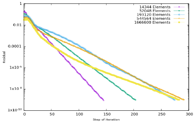
Figure 3: Convergence curves of the residual of dual equations.

As is shown in Figure 3, the solver for dual equations is steady and powerful. Even for the mesh with more than $1,500,000$ elements, the convergence trace of the solver is smooth, which supports the whole algorithm of the DWR refinement.

4.3 Numerical Algorithm

4.3.1 AFVM4CFD

In [25], a comprehensive review of the development of computational fluid dynamics in the past, as well as the perspective in the future 15 years has been delivered, in which the mesh adaptivity was listed as a potential technique for significantly enhancing the simulation efficiency. However, it was also mentioned that such a potential method has not seen widespread use, “due to issues related to software complexity, inadequate error estimation capabilities, and complex geometry”.

AFVM4CFD is a library maintained by our group for solving the steady Euler equations problem. In this library, we provide a competitive solution to resolve the above three issues in developing adaptive mesh methods for steady Euler equations through 1). a thorough investigation of the dual consistency in dual-weighted residual methods, 2). a well design of a dual-weighted residual based $h$-adaptive mesh method with dual consistency, based on a Newton-GMG numerical framework, and 3). a quality code based on AFVM4CFD library. It is worth mentioning that with the AFVM4CFD, the Euler equations can be solved well with a satisfactory residual that gets close to the machine precision. Now AFVM4CFD is under the application of software copyright.

4.3.2 $h$-adaptivity process

From the theoretical discussion above, we developed the DWR-based $h$-adaptive refinement with a Newton-GMG solver, which solved the equations well. The process for a one-step refinement can be summed up as the algorithm below:

Data: Initial $\mathcal{K}_{H}$, $TOL$

Result: $\mathcal{K}_{h}$

1 Using the Newton-GMG to solve $\mathcal{R}_{H}(\mathbf{u}_{0})=0$ with residual tolerance $1.0\times 10^{-3}$;

2 Reconstruct the piecewise constant solutions $\mathbf{u}_{1}=R^{0}_{1}\mathbf{u}_{0}$;

3 Interpolate solution $(\mathbf{u_{1}})_{H}$ from the mesh $\mathcal{K}_{H}$ to $\mathcal{K}_{h}$ to get $(\mathbf{u}_{1})_{h}^{H}$;

4 Record the residual $\mathcal{R}_{h}\left((\mathbf{u}_{1})_{h}^{H}\right)$;

5 Solve the dual equation to get $(\mathbf{z}_{0})_{H}$;

6 Calculate the error indicator for each element;

7 while $\mathcal{E}_{K_{H}}>TOL$ for some $K_{H}$ do

8       Adaptively refining the mesh $\mathcal{K}_{H}$ with the process in [14];

9 end while

Algorithm 1 DWR for one-step mesh refinement

In our previous work[14][11], we used a constant indicator for successive refinements process. However, as the desired precision of the quantity of interest increases, the number of elements in the mesh grows rapidly. Choosing an optimal indicator is tricky due to the reason that excessive refinement may need too much degree of freedom while inadequate refinement will cause too many steps for refinement and even lead to a significant error result. It has been suggested by [1] that tolerance shall match the error distribution histograms on hierarchical meshes. Besides, Nemec developed a decreasing threshold strategy based on the adjoint-based framework[22], which can help save degrees of freedom for a specific quantity of interest. Motivated by this idea, we have designed the algorithm with a decreasing refinement threshold, and the growth of grids has met expectations well.

5 Numerical Experiment

5.1 Subsonic model

To validate the efficiency of the algorithm, we tested the model with the following configurations:

• A domain with a NACA0012 airfoil, surrounding by an outer circle with a radius of 40;

• Mach number 0.5, and attack angle 0^∘;

• Lax-Friedrichs numerical flux;

• Drag coefficient as the quantity of interest, and zero normal velocity as the solid wall boundary condition.

Figure 4: Top: the isolines of the first and second dual momentum variables, with Dual-Consistent DWR method. Bottom: isolines with Dual-Inconsistent DWR method, respectively.

To compare the differences between dual consistency and dual inconsistency, we calculate the dual solutions using a mesh with four times uniform refinement. The drag coefficient can be chosen as the quantity of interest with zero normal velocity boundary conditions, resulting in no normal pressure on the airfoil boundary and a drag coefficient close to 0, i.e., $\mathcal{J}(\mathbf{u})=0$. As shown in Figure 4, the DWR method constructed on a dual-consistent framework generates symmetric and smooth dual solutions, while the dual solutions from the dual-inconsistent framework are oscillatory. This evidence demonstrates that the main difference between these two schemes is the impact on the dual solutions.

The whole algorithm works well when the dual solutions part is included in the calculation. The results of the convergence trace are shown in Figure 5.

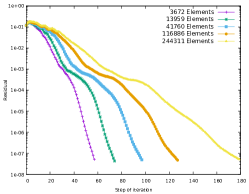
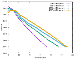
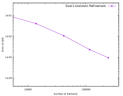
Figure 5: Convergence curves of Newton-GMG solver for the steady Euler equations with successive $h$-adaptivity. Left: the residual of primal equations; Middle: the residual of dual equations; Right: the error of quantity of interest.

Then, a dual-consistent DWR-based $h$-adaptivity algorithm is constructed in this framework. Further discussions about dual consistency are conducted based on this solver, and the results are shown with the following simulations.

5.2 Transonic model

• A domain with a NACA0012 airfoil, surrounding by an outer circle with a radius of 30;

• Mach number 0.8, and attack angle 0^∘;

• Lax-Friedrichs numerical flux;

• Drag coefficient as the quantity of interest, and mirror reflection as the solid wall boundary condition.

Since the solver for the primal equations is so effective that the residual of equations can converge to machine precision, we use a uniformly refined mesh with $3,672,064$ elements to calculate the quantity of interest, which is $C_{d}=9.42314\times 10^{-3}.$ Then we compared this with the same configurations but with a change in the dual consistency scheme, which produced the following results.

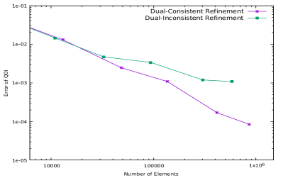
Figure 6: Convergence curves of dual-consistent refinement and dual-inconsistent refinement for NACA0012 with Mach number 0.8, attack angle 0^∘.

It is shown that the dual-consistent refinement preserves a stable convergence rate till the precision is below $1.0\times 10^{-4}$ while dual-inconsistent refinement converges to a result around $1.0\times 10^{-3}$ precision. Specifically, in this model, the error in a dual-consistent framework could converge to $1.08906\times 10^{-3}$ with $136,141$ elements, while the dual-inconsistent framework converges to $1.08446\times 10^{-3}$ with $581,701$ elements.

The dual-inconsistent method may refine areas that do not significantly influence the calculation of target functions, resulting in wasted degrees of freedom. As shown in Figure 6, the dual-consistent refinement with $100,000$ elements produced approximately equivalent to the dual-inconsistent refinement with nearly $600,000$ elements. The behaviour can be explained by the distribution of dual variables. In Figure 7, the first variable of dual solutions is symmetric from the dual-consistent solver while the dual-inconsistent one is non-symmetric and uneven. Then the dual-consistent solver refined the area around the boundary. The dual-inconsistent algorithm refined only the leading edge and around the shock waves. Even when the degree of freedom is increased for the dual-inconsistent solver, the quantity of interest cannot decrease under expectation.

Compared with the dual-inconsistent refinement, the dual-consistent scheme is always stable, enabling the quantity of interest to converge smoothly. The validity of this assertion has been bolstered through a series of empirical investigations conducted on various models, and the ensuing results are hereby presented in Figure 7.

Figure 7: Top: Left: the first dual variable from dual-consistent solver. Right: The refined mesh from dual-consistent solver. Bottom: Left: the first dual variable from dual-inconsistent solver. Right: The refined mesh from dual-inconsistent solver.

• A domain with a NACA0012 airfoil, surrounding by an outer circle with a radius of 30;

• Mach number 0.98, and attack angle 1.25^∘;

• Lax-Friedrichs numerical flux;

• Drag coefficient as the quantity of interest, and mirror reflection as the solid wall boundary condition.

In this example, we considered the influence of the attack angle. Since the boundary modification method can help us preserve the dual consistency for the reflection boundary condition, the difference between dual consistency and dual inconsistency is shown below.

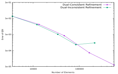
Figure 8: Convergence curves of dual-consistent refinement and dual-inconsistent refinement for NACA0012 with Mach number 0.98, attack angle 1.25^∘.

Even if the error calculated on final meshes derived from dual-consistent refinement and dual-inconsistent refinement have approximate precision, the dual-consistent refinement was more stable than dual-inconsistent refinement. This observation suggests that the accuracy of the quantity of interest improves as the element size increases under a dual-consistent framework. However, the convergence trace of a dual-inconsistent framework has oscillations as illustrated in Figure 8, not only wasting degrees of freedom but also influencing the analysis of the convergence of target functions. In order to gain a deeper understanding of the efficacy of the DWR method in yielding a stable rate of convergence with respect to the quantity of interest, we have presented a visual analysis of the dual solutions and residuals employed for the computation of the error indicators.

Figure 9: NACA0012 model, Mach number 0.98, attack angle 1.25^∘.: Left: Dual solution of the first variable for the indicators; Middle: Residual of the first variable for the indicators; Right: Meshes generated from the indicators.

As shown in Figure 9, the residuals of this model oscillated around the shock waves and the direction of the inflow area, while the dual solutions focused on the boundary of the airfoils. The error indicators from the DWR method balance both the residuals and the dual solutions, generating a mesh that could resolve the quantity of interest well.

The reason lead to the oscillations can be seen from Figure 10. The dual-consistent solver generated a smoothly refined mesh, both the effect of dual and residual are considered. Conversely, the dual-inconsistent solver generates the dual solutions unevenly. The effect of residual hasn’t been taken into account. Worse still, the refined areas are disperse. To test the robustness of the dual-consistent framework, we considered different models using the same algorithm in the following parts.

Figure 10: Top: Left: the isolines of the first dual variables from dual-consistent solver. Right: The refined mesh from dual-consistent solver. Bottom: Left: the isolines of the first dual variables from dual-inconsistent solver. Right: The refined mesh from dual-inconsistent solver.

• A domain with a RAE2822 airfoil, surrounding by an outer circle with a radius of 30;

• Mach number 0.729, and attack angle 2.31^∘;

• Lax-Friedrichs numerical flux;

• Drag coefficient as the quantity of interest, and mirror reflection as the solid wall boundary condition.

Similarly, we use a uniformly refined mesh with $3,801,088$ elements to calculate the quantity of interest, which is $C_{d}=1.44349\times 10^{-2}.$ The dual-consistent framework still works well for the whole algorithm.

Figure 11: RAE2822 model: Left: Dual solution of the first variable for the indicators; Middle: Residual of the first variable for the indicators; Right: Meshes generated from the indicators.

Figure 12: RAE2822 refined mesh: Left: The first time adaptation; Middle: The third time adaptation; Right: The fifth time adaptation.

Unlike the residual-based adaptation, which emphasizes refinement around shock waves, the DWR method aims to solve the quantity of interest with the least computational cost. In this example, Figure 11 shows that the dual equations concentrate on the top half area of the airfoil, while the residuals oscillate around the shock waves and outflow direction. The DWR method combines these two aspects to produce a stable error reduction trace of the target function. During the adaptation process, as shown in Figure 12, the refinement areas focus on the top half at beginning. With the iteration continued, the refinement part concentrated around the residual as well. The result is shown in Figure 13.

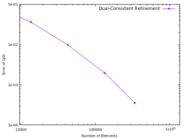
Figure 13: Convergence curves of dual-consistent refinement for RAE2822 with Mach number 0.729, attack angle 2.31^∘.

• A domain with two NACA0012 airfoils, surrounding by an outer circle with a radius of 30;

• Mach number 0.8, and attack angle 0^∘;

• Lax-Friedrichs numerical flux;

• Drag coefficient of different airfoils, and mirror reflection as the solid wall boundary condition.

Figure 14: Two bodies model: Left: Dual solution of the first variable for the indicators; Middle: Residual of the first variable for the indicators; Right: Meshes generated from the indicators.

Initially, we chose the quantity of interest as the drag coefficient of the upper airfoil. Figure 10 exhibits that the dual solutions concentrate on the boundary of the upper airfoil, while the residuals of different variables have oscillations around the shock waves and the outflow direction. The meshes generated from the error indicators predominantly refine the upper airfoil. In contrast, the elements refined around the lower airfoil behave like a residual-based adaptation since the dual equations make no contributions in that region. The upper airfoil took a balance between the dual solutions and the residuals, resulting in a stable convergence of the quantity of interest. Similarly, the quantity of interest is calculated on a mesh with $2,227,712$ elements, then $C_{d}=9.218816\times 10^{-3}.$

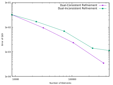
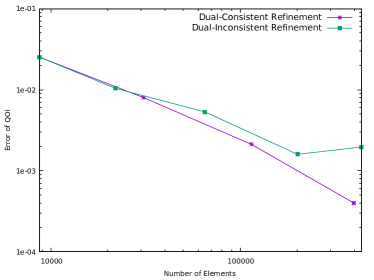
Figure 15: Convergence curves of dual-consistent and dual-inconsistent refinement for Two bodies NACA0012 with Mach number 0.8, attack angle 0^∘. Left: The drag of the upper airfoil chosen as the quantity of interest. Right: The drag of the lower airfoil chosen as the quantity of interest.

If the quantity of interest is chosen as the lower airfoil, the refinement behavior is reversed, with the meshes generated from the error indicators mainly focusing on the lower airfoil.

Figure 16: Two bodies model: Left: Dual solution of the first variable for the indicators; Middle: Residual of the first variable for the indicators; Right: Meshes generated from the indicators.

The convergence curves for the two examples demonstrate that dual-consistent refinement is more stable than dual-inconsistent refinement, which can result in unexpected oscillations. More importantly, even if dual-inconsistent DWR may produce a quantity of interest with an acceptable level of precision, it is not always robust enough to derive a satisfactory stopping criterion for target functional-based adaptation.

6 Conclusion

Based on previous works, we further constructed a dual-consistent DWR-based $h$-adaptivity method for the steady Euler equations in the AFVM4CFD package. Implementing the Newton method for nonlinear equations posed a challenge for $h$-adaptivity, but we validated the efficiency of dual consistency property using the Newton-GMG solver. The following features can be observed from satisfying numerical results, that i). the dual equations can be solved smoothly with residuals approaching machine accuracy. ii). a stable convergence of the quantity of interest can be obtained in all numerical experiments, and iii). a saving on mesh grids by orders of magnitude can be achieved for calculating the quantity of interest with a given requirement on the accuracy, compared with the DWR-based h-adaptive method without the dual-consistency.

For implementing issues, developing a suitable tolerance for the adaptivity process is still tricky. In order to choose a suitable tolerance for the adaptation, numerous numerical experiments should be conducted. To make the whole process for refinement more automatic, we plan to develop an algorithm to balance the tolerance based on the mesh. Besides, obtaining the dual solutions still requires a uniformly refined mesh from the previous step, which we hope to improve upon. Given that the dual equations are linear and do not demand high precision to determine the error indicators, we plan to incorporate machine learning or a multiple precision method to improve efficiency. We are now constructing the convolutional neural networks form dual solver which can saves the time for an order of magnitude. In the training process, we find that the dual consistency is still an important issue that influence the adaptation performance. Moreover, since the motivation of the DWR based $h$-adaptivity is from practical issues, the shape optimization techniques shall be discussed in the future. Finally, the dual consistency property for supersonic modeling is still under development.

CRediT authorship contribution statement

Jingfeng Wang: Formal analysis, Methodology, Software, Writing - original draft. Guanghui Hu: Conceptualization, Methodology, Software, Supervision, Writing - review & editing.

Declaration of competing interest

The authors declare that they have no known competing financial interests or personal relationships that could have appeared to influence the work reported in this paper.

References

- [1] Michael Aftosmis and Marsha Berger. Multilevel error estimation and adaptive h-refinement for Cartesian meshes with embedded boundaries. In 40th AIAA Aerospace Sciences Meeting & Exhibit, page 863, 2002.
- [2] Timothy Barth and Mats Larson. A posteriori error estimates for higher order Godunov finite volume methods on unstructured meshes. Finite Volumes for Complex Applications III, London, 2002.
- [3] Vít Dolejší and Filip Roskovec. Goal-oriented error estimates including algebraic errors in discontinuous Galerkin discretizations of linear boundary value problems. Applications of Mathematics, 62(6):579–605, 2017.
- [4] Vít Dolejší and Filip Roskovec. Goal-oriented anisotropic hp-adaptive discontinuous Galerkin method for the Euler equations. Communications on Applied Mathematics and Computation, 4:143–179, 2022.
- [5] Krzysztof Fidkowski and David Darmofal. Review of output-based error estimation and mesh adaptation in computational fluid dynamics. AIAA journal, 49(4):673–694, 2011.
- [6] Michael Giles and Niles Pierce. Adjoint equations in CFD-Duality, boundary conditions and solution behaviour. In 13th Computational Fluid Dynamics Conference, page 1850, 1997.
- [7] Kathryn Harriman, David Gavaghan, and Endre Suli. The importance of adjoint consistency in the approximation of linear functionals using the discontinuous galerkin finite element method. 2004.
- [8] Ralf Hartmann. Adjoint consistency analysis of discontinuous Galerkin discretizations. SIAM Journal on Numerical Analysis, 45(6):2671–2696, 2007.
- [9] Ralf Hartmann and Tobias Leicht. Generalized adjoint consistent treatment of wall boundary conditions for compressible flows. Journal of Computational Physics, 300:754–778, 2015.
- [10] Jason Hicken and David Zingg. Dual consistency and functional accuracy: a finite-difference perspective. Journal of Computational Physics, 256:161–182, 2014.
- [11] Guanghui Hu. An adaptive finite volume method for 2D steady Euler equations with WENO reconstruction. Journal of Computational Physics, 252:591–605, 2013.
- [12] Guanghui Hu, Ruo Li, and Tao Tang. A robust WENO type finite volume solver for steady Euler equations on unstructured grids. Communications in Computational Physics, 9(3):627–648, 2011.
- [13] Guanghui Hu, Xucheng Meng, and Nianyu Yi. Adjoint-based an adaptive finite volume method for steady Euler equations with non-oscillatory k-exact reconstruction. Computers & Fluids, 139:174–183, 2016.
- [14] Guanghui Hu and Nianyu Yi. An adaptive finite volume solver for steady Euler equations with non-oscillatory k-exact reconstruction. Journal of Computational Physics, 312:235–251, 2016.
- [15] Gaetan Kenway, Charles Mader, Ping He, and Joaquim Martins. Effective adjoint approaches for computational fluid dynamics. Progress in Aerospace Sciences, 110:100542, 2019.
- [16] Boya Li. Newton linearized methods for semilinear parabolic equations. Numerical Mathematics-theory Methods and Applications, 13:928–945, 2020.
- [17] Ruo Li, Xin Wang, and Weibo Zhao. A multigrid block LU-SGS algorithm for Euler equations on unstructured grids. Numerical Mathematics: Theory, Methods and Applications, 1:92–112, 2008.
- [18] Ruo Li and Wei Zhong. A modified adaptive improved mapped weno method. Communications in Computational Physics, 30(5):1545–1588, 2021.
- [19] Yangyang Liu, Liming Yang, Chang Shu, and Huangwei Zhang. A multi-dimensional shock-capturing limiter for high-order least square-based finite difference-finite volume method on unstructured grids. Advances in Applied Mathematics and Mechanics, 13(3):671–700, 2020.
- [20] James Lu. An a posteriori error control framework for adaptive precision optimization using discontinuous Galerkin finite element method. PhD thesis, Massachusetts Institute of Technology, 2005.
- [21] Xucheng Meng, Yaguang Gu, and Guanghui Hu. A Fourth-Order Unstructured NURBS-Enhanced finite volume WENO Scheme for Steady Euler Equations in Curved Geometries. Communications on Applied Mathematics and Computation, pages 1–28, 2021.
- [22] Marian Nemec, Michael Aftosmis, and Mathias Wintzer. Adjoint-based adaptive mesh refinement for complex geometries. In 46th AIAA Aerospace Sciences Meeting and Exhibit, page 725, 2008.
- [23] Niles Pierce and Michael Giles. Adjoint recovery of superconvergent functionals from PDE approximations. SIAM review, 42(2):247–264, 2000.
- [24] Ajay Rangarajan, Georg May, and Vit Dolejsi. Adjoint-based anisotropic hp-adaptation for discontinuous galerkin methods using a continuous mesh model. Journal of Computational Physics, 409:109321, 2020.
- [25] Jeffrey Slotnick, Abdollah Khodadoust, Juan Alonso, David Darmofal, William Gropp, Elizabeth Lurie, and Dimitri Mavriplis. CFD vision 2030 study: a path to revolutionary computational aerosciences. Technical report, 2014.
- [26] David Venditti and David Darmofal. Adjoint error estimation and grid adaptation for functional outputs: Application to quasi-one-dimensional flow. Journal of Computational Physics, 164(1):204–227, 2000.
- [27] David Venditti and David Darmofal. Grid adaptation for functional outputs: application to two-dimensional inviscid flows. Journal of Computational Physics, 176(1):40–69, 2002.
- [28] Shuhai Zhang, Shufen Jiang, and Chi-Wang Shu. Improvement of convergence to steady state solutions of Euler equations with the WENO schemes. Journal of Scientific Computing, 47(2):216–238, 2011.