Compressed Decentralized Proximal Stochastic Gradient Method for Nonconvex Composite Problems with Heterogeneous Data

Abstract

We first propose a decentralized proximal stochastic gradient tracking method (DProxSGT) for nonconvex stochastic composite problems, with data heterogeneously distributed on multiple workers in a decentralized connected network. To save communication cost, we then extend DProxSGT to a compressed method by compressing the communicated information. Both methods need only $\mathcal{O}(1)$ samples per worker for each proximal update, which is important to achieve good generalization performance on training deep neural networks. With a smoothness condition on the expected loss function (but not on each sample function), the proposed methods can achieve an optimal sample complexity result to produce a near-stationary point. Numerical experiments on training neural networks demonstrate the significantly better generalization performance of our methods over large-batch training methods and momentum variance-reduction methods and also, the ability of handling heterogeneous data by the gradient tracking scheme.

1 Introduction

In this paper, we consider to solve nonconvex stochastic composite problems in a decentralized setting:

$$\min_{{\mathbf{x}}\in\mathbb{R}^{d}}\phi({\mathbf{x}})=f({\mathbf{x}})+r({\mathbf{x}}),$$ (1)

$$\text{with }f({\mathbf{x}})=\frac{1}{n}\sum_{i=1}^{n}f_{i}({\mathbf{x}}),f_{i}({\mathbf{x}})\!=\!\mathbb{E}_{\xi_{i}\sim\mathcal{D}_{i}}[F_{i}({\mathbf{x}},\xi_{i})].$$

Here, $\{\mathcal{D}_{i}\}_{i=1}^{n}$ are possibly non-i.i.d data distributions on $n$ machines/workers that can be viewed as nodes of a connected graph $\mathcal{G}$, and each $F_{i}(\cdot,\xi_{i})$ can only be accessed by the $i$-th worker. We are interested in problems that satisfy the following structural assumption.

Assumption 1 (Problem structure).

We assume that

• $r$ is closed convex and possibly nondifferentiable.

• Each $f_{i}$ is $L$-smooth in ${\mathrm{dom}}(r)$, i.e., $\|\nabla f_{i}({\mathbf{x}})-\nabla f_{i}({\mathbf{y}})\|\leq L\|{\mathbf{x}}-{\mathbf{y}}\|$, for any ${\mathbf{x}},{\mathbf{y}}\in{\mathrm{dom}}(r)$.

• $\phi$ is lower bounded, i.e., $\phi^{*}\triangleq\min_{\mathbf{x}}\phi({\mathbf{x}})>-\infty$.

Let $\mathcal{N}=\{1,2,\ldots,n\}$ be the set of nodes of $\mathcal{G}$ and $\mathcal{E}$ the set of edges. For each $i\in\mathcal{N}$, denote $\mathcal{N}_{i}$ as the neighbors of worker $i$ and itself, i.e., $\mathcal{N}_{i}=\{j:(i,j)\in\mathcal{E}\}\cup\{i\}$. Every worker can only communicate with its neighbors. To solve (1) collaboratively, each worker $i$ maintains a copy, denoted as ${\mathbf{x}}_{i}$, of the variable ${\mathbf{x}}$. With these notations, (1) can be formulated equivalently to

$$\begin{split}\min_{\mathbf{X}\in\mathbb{R}^{d\times n}}&\frac{1}{n}\sum_{i=1}^{n}\phi_{i}({\mathbf{x}}_{i}),\text{with }\phi_{i}({\mathbf{x}}_{i})\triangleq f_{i}({\mathbf{x}}_{i})+r({\mathbf{x}}_{i}),\\ \mbox{s.t. }\quad&{\mathbf{x}}_{i}={\mathbf{x}}_{j},\forall\,j\in\mathcal{N}_{i},\forall\,i=1,\ldots,n.\end{split}$$ (2)

Problems with a nonsmooth regularizer, i.e., in the form of (1), appear in many applications such as $\ell_{1}$-regularized signal recovery (Eldar & Mendelson, 2014; Duchi & Ruan, 2019), online nonnegative matrix factorization (Guan et al., 2012), and training sparse neural networks (Scardapane et al., 2017; Yang et al., 2020). When data involved in these applications are distributed onto (or collected by workers on) a decentralized network, it necessitates the design of decentralized algorithms.

Although decentralized optimization has attracted a lot of research interests in recent years, most existing works focus on strongly convex problems (Scaman et al., 2017; Koloskova et al., 2019b) or convex problems (Tsianos et al., 2012; Taheri et al., 2020) or smooth nonconvex problems (Bianchi & Jakubowicz, 2012; Di Lorenzo & Scutari, 2016; Wai et al., 2017; Lian et al., 2017; Zeng & Yin, 2018). Few works have studied nonsmooth nonconvex decentralized stochastic optimization like (2) that we consider. (Chen et al., 2021; Xin et al., 2021a; Mancino-Ball et al., 2022) are among the exceptions. However, they either require to take many data samples for each update or assume a so-called mean-squared smoothness condition, which is stronger than the smoothness condition in Assumption 1(ii), in order to perform momentum-based variance-reduction step. Though these methods can have convergence (rate) guarantee, they often yield poor generalization performance on training deep neural networks, as demonstrated in (LeCun et al., 2012; Keskar et al., 2016) for large-batch training methods and in our numerical experiments for momentum variance-reduction methods.

On the other side, many distributed optimization methods (Shamir & Srebro, 2014; Lian et al., 2017; Wang & Joshi, 2018) often assume that the data are i.i.d across the workers. However, this assumption does not hold in many real-world scenarios, for instance, due to data privacy issue that local data has to stay on-premise. Data heterogeneity can result in significant degradation of the performance by these methods. Though some papers do not assume i.i.d. data, they require certain data similarity, such as bounded stochastic gradients (Koloskova et al., 2019b, a; Taheri et al., 2020) and bounded gradient dissimilarity (Tang et al., 2018a; Assran et al., 2019; Tang et al., 2019a; Vogels et al., 2020).

To address the critical practical issues mentioned above, we propose a decentralized proximal stochastic gradient tracking method that needs only a single or $O(1)$ data samples (per worker) for each update. With no assumption on data similarity, it can still achieve the optimal convergence rate on solving problems satisfying conditions in Assumption 1 and yield good generalization performance. In addition, to reduce communication cost, we give a compressed version of the proposed algorithm, by performing compression on the communicated information. The compressed algorithm can inherit the benefits of its non-compressed counterpart.

1.1 Our Contributions

Our contributions are three-fold. First, we propose two decentralized algorithms, one without compression (named DProxSGT) and the other with compression (named CDProxSGT), for solving decentralized nonconvex nonsmooth stochastic problems. Different from existing methods, e.g., (Xin et al., 2021a; Wang et al., 2021b; Mancino-Ball et al., 2022), which need a very large batchsize and/or perform momentum-based variance reduction to handle the challenge from the nonsmooth term, DProxSGT needs only $\mathcal{O}(1)$ data samples for each update, without performing variance reduction. The use of a small batch and a standard proximal gradient update enables our method to achieve significantly better generalization performance over the existing methods, as we demonstrate on training neural networks. To the best of our knowledge, CDProxSGT is the first decentralized algorithm that applies a compression scheme for solving nonconvex nonsmooth stochastic problems, and it inherits the advantages of the non-compressed method DProxSGT. Even applied to the special class of smooth nonconvex problems, CDProxSGT can perform significantly better over state-of-the-art methods, in terms of generalization and handling data heterogeneity.

Second, we establish an optimal sample complexity result of DProxSGT, which matches the lower bound result in (Arjevani et al., 2022) in terms of the dependence on a target tolerance $\epsilon$, to produce an $\epsilon$-stationary solution. Due to the coexistence of nonconvexity, nonsmoothness, big stochasticity variance (due to the small batch and no use of variance reduction for better generalization), and decentralization, the analysis is highly non-trivial. We employ the tool of Moreau envelope and construct a decreasing Lyapunov function by carefully controlling the errors introduced by stochasticity and decentralization.

Third, we establish the iteration complexity result of the proposed compressed method CDProxSGT, which is in the same order as that for DProxSGT and thus also optimal in terms of the dependence on a target tolerance. The analysis builds on that of DProxSGT but is more challenging due to the additional compression error and the use of gradient tracking. Nevertheless, we obtain our results by making the same (or even weaker) assumptions as those assumed by state-of-the-art methods (Koloskova et al., 2019a; Zhao et al., 2022).

1.2 Notation

For any vector ${\mathbf{x}}\in\mathbb{R}^{d}$, we use $\|{\mathbf{x}}\|$ for the $\ell_{2}$ norm. For any matrix $\mathbf{A}$, $\|\mathbf{A}\|$ denotes the Frobenius norm and $\|\mathbf{A}\|_{2}$ the spectral norm. $\mathbf{X}=[{\mathbf{x}}_{1},{\mathbf{x}}_{2},\ldots,{\mathbf{x}}_{n}]\in\mathbb{R}^{d\times n}$ concatinates all local variables. The superscript ^t will be used for iteration or communication. $\nabla F_{i}({\mathbf{x}}_{i}^{t},\xi_{i}^{t})$ denotes a local stochastic gradient of $F_{i}$ at ${\mathbf{x}}_{i}^{t}$ with a random sample $\xi_{i}^{t}$. The column concatenation of $\{\nabla F_{i}({\mathbf{x}}_{i}^{t},\xi_{i}^{t})\}$ is denoted as

$$\nabla\mathbf{F}^{t}=\nabla\mathbf{F}(\mathbf{X}^{t},\Xi^{t})=[\nabla F_{1}({\mathbf{x}}_{1}^{t},\xi_{1}^{t}),\ldots,\nabla F_{n}({\mathbf{x}}_{n}^{t},\xi_{n}^{t})],\vspace{-0.1cm}$$

where $\Xi^{t}=[\xi_{1}^{t},\xi_{2}^{t},\ldots,\xi_{n}^{t}]$. Similarly, we denote

$$\nabla\mathbf{f}^{t}=[\nabla f_{1}({\mathbf{x}}_{1}^{t}),\ldots,\nabla f_{n}({\mathbf{x}}_{n}^{t})].\vspace{-0.1cm}$$

For any $\mathbf{X}\in\mathbb{R}^{d\times n}$, we define

$$\bar{{\mathbf{x}}}=\textstyle\frac{1}{n}\mathbf{X}\mathbf{1},\quad\overline{\mathbf{X}}=\mathbf{X}\mathbf{J}=\bar{{\mathbf{x}}}\mathbf{1}^{\top},\quad\mathbf{X}_{\perp}=\mathbf{X}(\mathbf{I}-\mathbf{J}),\vspace{-0.1cm}$$

where $\mathbf{1}$ is the all-one vector, and $\mathbf{J}=\frac{\mathbf{1}\mathbf{1}^{\top}}{n}$ is the averaging matrix. Similarly, we define the mean vectors

$$\overline{\nabla}\mathbf{F}^{t}=\textstyle\frac{1}{n}\mathbf{F}^{t}\mathbf{1},\ \overline{\nabla}\mathbf{f}^{t}=\textstyle\frac{1}{n}\mathbf{f}^{t}\mathbf{1}.\vspace{-0.1cm}$$

We will use $\mathbb{E}_{t}$ for the expectation about the random samples $\Xi^{t}$ at the $t$th iteration and $\mathbb{E}$ for the full expectation. $\mathbb{E}_{Q}$ denotes the expectation about a stochastic compressor $Q$.

2 Related Works

The literature of decentralized optimization has been growing vastly. To exhaust the literature is impossible. Below we review existing works on decentralized algorithms for solving nonconvex problems, with or without using a compression technique. For ease of understanding the difference of our methods from existing ones, we compare to a few relevant methods in Table 1.

Table 1: Comparison between our methods and some relevant methods: ProxGT-SA and ProxGT-SR-O in (Xin et al., 2021a), DEEPSTORM (Mancino-Ball et al., 2022), ChocoSGD (Koloskova et al., 2019a), and BEER (Zhao et al., 2022). We use “CMP” to represent whether compression is performed by a method. GRADIENTS represents additional assumptions on the stochastic gradients in addition to those made in Assumption 3. SMOOTHNESS represents the smoothness condition, where “mean-squared” means $\mathbb{E}_{\xi_{i}}[\|\nabla F_{i}({\mathbf{x}};\xi_{i})-\nabla F_{i}({\mathbf{y}};\xi_{i})\|^{2}]\leq L^{2}\|{\mathbf{x}}-{\mathbf{y}}\|^{2}$ that is stronger than the $L$-smoothness of $f_{i}$. BS is the required batchsize to get an $\epsilon$-stationary solution. VR and MMT represent whether the variance reduction or momentum are used. Large batchsize and/or momentum variance reduction can degrade the generalization performance, as we demonstrate in numerical experiments.

Methods	CMP	$r\not\equiv 0$	GRADIENTS	SMOOTHNESS	(BS, VR, MMT)
ProxGT-SA	No	Yes	No	$f_{i}$ is smooth	($\mathcal{O}(\frac{1}{\epsilon^{2}})$, No , No)
ProxGT-SR-O	No	Yes	No	mean-squared	($\mathcal{O}(\frac{1}{\epsilon})$, Yes, No)
DEEPSTORM	No	Yes	No	mean-squared	($\mathcal{O}(1)$, Yes, Yes)
DProxSGT (this paper)	No	Yes	No	$f_{i}$ is smooth	($\mathcal{O}(1)$, No, No)
ChocoSGD	Yes	No	$\mathbb{E}_{\xi}[\|\nabla F_{i}({\mathbf{x}},\xi_{i})\|^{2}]\leq G^{2}$	$f_{i}$ is smooth	($\mathcal{O}(1)$, No, No)
BEER	Yes	No	No	$f$ is smooth	($\mathcal{O}(\frac{1}{\epsilon^{2}})$, No, No)
CDProxSGT (this paper)	Yes	Yes	No	$f_{i}$ is smooth	($\mathcal{O}(1)$, No, No)

2.1 Non-compressed Decentralized Methods

For nonconvex decentralized problems with a nonsmooth regularizer, a lot of deterministic decentralized methods have been studied, e.g., (Di Lorenzo & Scutari, 2016; Wai et al., 2017; Zeng & Yin, 2018; Chen et al., 2021; Scutari & Sun, 2019). When only stochastic gradient is available, a majority of existing works focus on smooth cases without a regularizer or a hard constraint, such as (Lian et al., 2017; Assran et al., 2019; Tang et al., 2018b), gradient tracking based methods (Lu et al., 2019; Zhang & You, 2019; Koloskova et al., 2021), and momentum-based variance reduction methods (Xin et al., 2021b; Zhang et al., 2021). Several works such as (Bianchi & Jakubowicz, 2012; Wang et al., 2021b; Xin et al., 2021a; Mancino-Ball et al., 2022) have studied stochastic decentralized methods for problems with a nonsmooth term $r$. However, they either consider some special $r$ or require a large batch size. (Bianchi & Jakubowicz, 2012) considers the case where $r$ is an indicator function of a compact convex set. Also, it requires bounded stochastic gradients. (Wang et al., 2021b) focuses on problems with a polyhedral $r$, and it requires a large batch size of $\mathcal{O}(\frac{1}{\epsilon})$ to produce an (expected) $\epsilon$-stationary point. (Xin et al., 2021a; Mancino-Ball et al., 2022) are the most closely related to our methods. To produce an (expected) $\epsilon$-stationary point, the methods in (Xin et al., 2021a) require a large batch size, either $\mathcal{O}(\frac{1}{\epsilon^{2}})$ or $\mathcal{O}(\frac{1}{\epsilon})$ if variance reduction is applied. The method in (Mancino-Ball et al., 2022) requires only $\mathcal{O}(1)$ samples for each update by taking a momentum-type variance reduction scheme. However, in order to reduce variance, it needs a stronger mean-squared smoothness assumption. In addition, the momentum variance reduction step can often hurt the generalization performance on training complex neural networks, as we will demonstrate in our numerical experiments.

2.2 Compressed Distributed Methods

Communication efficiency is a crucial factor when designing a distributed optimization strategy. The current machine learning paradigm oftentimes resorts to models with a large number of parameters, which indicates a high communication cost when the models or gradients are transferred from workers to the parameter server or among workers. This may incur significant latency in training. Hence, communication-efficient algorithms by model or gradient compression have been actively sought.

Two major groups of compression operators are quantization and sparsification. The quantization approaches include 1-bit SGD (Seide et al., 2014), SignSGD (Bernstein et al., 2018), QSGD (Alistarh et al., 2017), TernGrad (Wen et al., 2017). The sparsification approaches include Random-$k$ (Stich et al., 2018), Top-$k$ (Aji & Heafield, 2017), Threshold-$v$ (Dutta et al., 2019) and ScaleCom (Chen et al., 2020). Direct compression may slow down the convergence especially when compression ratio is high. Error compensation or error-feedback can mitigate the effect by saving the compression error in one communication step and compensating it in the next communication step before another compression (Seide et al., 2014). These compression operators are first designed to compress the gradients in the centralized setting (Tang et al., 2019b; Karimireddy et al., 2019).

The compression can also be applied to the decentralized setting for smooth problems, i.e., (2) with $r=0$. (Tang et al., 2019a) applies the compression with error compensation to the communication of model parameters in the decentralized seeting. Choco-Gossip (Koloskova et al., 2019b) is another communication way to mitigate the slow down effect from compression. It does not compress the model parameters but a residue between model parameters and its estimation. Choco-SGD uses Choco-Gossip to solve (2). BEER (Zhao et al., 2022) includes gradient tracking and compresses both tracked stochastic gradients and model parameters in each iteration by the Choco-Gossip. BEER needs a large batchsize of $\mathcal{O}(\frac{1}{\epsilon^{2}})$ in order to produce an $\epsilon$-stationary solution. DoCoM-SGT(Yau & Wai, 2022) does similar updates as BEER but with a momentum term for the update of the tracked gradients, and it only needs an $\mathcal{O}(1)$ batchsize.

Our proposed CDProxSGT is for solving decentralized problems in the form of (2) with a nonsmooth $r({\mathbf{x}})$. To the best of our knowledge, CDProxSGT is the first compressed decentralized method for nonsmooth nonconvex problems without the use of a large batchsize, and it can achieve an optimal sample complexity without the assumption of data similarity or gradient boundedness.

3 Decentralized Algorithms

In this section, we give our decentralized algorithms for solving (2) or equivalently (1). To perform neighbor communications, we introduce a mixing (or gossip) matrix $\mathbf{W}$ that satisfies the following standard assumption.

Assumption 2 (Mixing matrix).

We choose a mixing matrix $\mathbf{W}$ such that

1. $\mathbf{W}$ is doubly stochastic: $\mathbf{W}\mathbf{1}=\mathbf{1}$ and $\mathbf{1}^{\top}\mathbf{W}=\mathbf{1}^{\top}$;

2. $\mathbf{W}_{ij}=0$ if $i$ and $j$ are not neighbors to each other;

3. $\mathrm{Null}(\mathbf{W}-\mathbf{I})=\mathrm{span}\{\mathbf{1}\}$ and $\rho\triangleq\|\mathbf{W}-\mathbf{J}\|_{2}<1$.

The condition in (ii) above is enforced so that direct communications can be made only if two nodes (or workers) are immediate (or 1-hop) neighbors of each other. The condition in (iii) can hold if the graph $\mathcal{G}$ is connected. The assumption $\rho<1$ is critical to ensure contraction of consensus error.

The value of $\rho$ depends on the graph topology. (Koloskova et al., 2019b) gives three commonly used examples: when uniform weights are used between nodes, $\mathbf{W}=\mathbf{J}$ and $\rho=0$ for a fully-connected graph (in which case, our algorithms will reduce to centralized methods), $1-\rho=\Theta(\frac{1}{n})$ for a 2d torus grid graph where every node has 4 neighbors, and $1-\rho=\Theta(\frac{1}{n^{2}})$ for a ring-structured graph. More examples can be found in (Nedić et al., 2018).

3.1 Non-compreseed Method

With the mixing matrix $\mathbf{W}$, we propose a decentralized proximal stochastic gradient method with gradient tracking (DProxSGT) for (2). The pseudocode is shown in Algorithm 1. In every iteration $t$, each node $i$ first computes a local stochastic gradient $\nabla F_{i}({\mathbf{x}}_{i}^{t},\xi_{i}^{t})$ by taking a sample $\xi_{i}^{t}$ from its local data distribution $\mathcal{D}_{i}$, then performs gradient tracking in (3) and neighbor communications of the tracked gradient in (4), and finally takes a proximal gradient step in (5) and mixes the model parameter with its neighbors in (6).

Algorithm 1 DProxSGT

  Initialize ${\mathbf{x}}_{i}^{0}$ and set ${\mathbf{y}}_{i}^{-1}=\mathbf{0}$, $\nabla F_{i}({\mathbf{x}}_{i}^{-1},\xi_{i}^{-1})=\mathbf{0}$, $\forall i\in\mathcal{N}$.

  for $t=0,1,2,\ldots,T-1$ do

     all nodes $i=1,2,\ldots,n$ do the updates in parallel:

     obtain one random sample $\xi_{i}^{t}$, compute a stochastic gradient $\nabla F_{i}({\mathbf{x}}_{i}^{t},\xi_{i}^{t})$, and perform

$${\mathbf{y}}_{i}^{t-\frac{1}{2}}={\mathbf{y}}_{i}^{t-1}+\nabla F_{i}({\mathbf{x}}_{i}^{t},\xi_{i}^{t})-\nabla F_{i}({\mathbf{x}}_{i}^{t-1},\xi_{i}^{t-1}),$$ (3)

$${\mathbf{y}}_{i}^{t}=\textstyle\sum_{j=1}^{n}\mathbf{W}_{ji}{\mathbf{y}}_{j}^{t-\frac{1}{2}},$$ (4)

$${\mathbf{x}}_{i}^{t+\frac{1}{2}}={\mathbf{Prox}}_{\eta r}\left({\mathbf{x}}_{i}^{t}-\eta{\mathbf{y}}_{i}^{t}\right),$$ (5)

$${\mathbf{x}}_{i}^{t+1}=\textstyle\sum_{j=1}^{n}\mathbf{W}_{ji}{\mathbf{x}}_{j}^{t+\frac{1}{2}}.\vspace{-0.2cm}$$ (6)

  end for

Note that for simplicity, we take only one random sample $\xi_{i}^{t}$ in Algorithm 1 but in general, a mini-batch of random samples can be taken, and all theoretical results that we will establish in the next section still hold. We emphasize that we need only $\mathcal{O}(1)$ samples for each update. This is different from ProxGT-SA in (Xin et al., 2021a), which shares a similar update formula as our algorithm but needs a very big batch of samples, as many as $\mathcal{O}(\frac{1}{\epsilon^{2}})$, where $\epsilon$ is a target tolerance. A small-batch training can usually generalize better than a big-batch one (LeCun et al., 2012; Keskar et al., 2016) on training large-scale deep learning models. Throughout the paper, we make the following standard assumption on the stochastic gradients.

Assumption 3 (Stochastic gradients).

We assume that

• The random samples $\{\xi_{i}^{t}\}_{i\in\mathcal{N},t\geq 0}$ are independent.

• There exists a finite number $\sigma\geq 0$ such that for any $i\in\mathcal{N}$ and ${\mathbf{x}}_{i}\in{\mathrm{dom}}(r)$,

  $$\mathbb{E}_{\xi_{i}}[\nabla F_{i}({\mathbf{x}}_{i},\xi_{i})]=\nabla f_{i}({\mathbf{x}}_{i}),$$

  $$\mathbb{E}_{\xi_{i}}[\|\nabla F_{i}({\mathbf{x}}_{i},\xi_{i})-\nabla f_{i}({\mathbf{x}}_{i})\|^{2}]\leq\sigma^{2}.$$

The gradient tracking step in (3) is critical to handle heterogeneous data (Di Lorenzo & Scutari, 2016; Nedic et al., 2017; Lu et al., 2019; Pu & Nedić, 2020; Sun et al., 2020; Xin et al., 2021a; Song et al., 2021; Mancino-Ball et al., 2022; Zhao et al., 2022; Yau & Wai, 2022; Song et al., 2022). In a deterministic scenario where $\nabla f_{i}(\cdot)$ is used instead of $\nabla F_{i}(\cdot,\xi)$, for each $i$, the tracked gradient ${\mathbf{y}}_{i}^{t}$ can converge to the gradient of the global function $\frac{1}{n}\sum_{i=1}^{n}f_{i}(\cdot)$ at $\bar{\mathbf{x}}^{t}$, and thus all local updates move towards a direction to minimize the global objective. When stochastic gradients are used, the gradient tracking can play a similar role and make ${\mathbf{y}}_{i}^{t}$ approach to the stochastic gradient of the global function. With this nice property of gradient tracking, we can guarantee convergence without strong assumptions that are made in existing works, such as bounded gradients (Koloskova et al., 2019b, a; Taheri et al., 2020; Singh et al., 2021) and bounded data similarity over nodes (Lian et al., 2017; Tang et al., 2018a, 2019a; Vogels et al., 2020; Wang et al., 2021a).

3.2 Compressed Method

In DProxSGT, each worker needs to communicate both the model parameter and tracked stochastic gradient with its neighbors at every iteration. Communications have become a bottleneck for distributed training on GPUs. In order to save the communication cost, we further propose a compressed version of DProxSGT, named CDProxSGT. The pseudocode is shown in Algorithm 2, where $Q_{\mathbf{x}}$ and $Q_{\mathbf{y}}$ are two compression operators.

Algorithm 2 CDProxSGT

  Initialize ${\mathbf{x}}_{i}^{0}$; set ${\mathbf{y}}_{i}^{-1}=\underline{{\mathbf{y}}}_{i}^{-1}=\nabla F_{i}({\mathbf{x}}_{i}^{-1},\xi_{i}^{-1})=\underline{{\mathbf{x}}}_{i}^{0}=\mathbf{0}$, $\forall i\in\mathcal{N}$.

  for $t=0,1,2,\ldots,T-1$ do

     all nodes $i=1,2,\ldots,n$ do the updates in parallel:

$${\mathbf{y}}_{i}^{t-\frac{1}{2}}={\mathbf{y}}_{i}^{t-1}+\nabla F_{i}({\mathbf{x}}_{i}^{t},\xi_{i}^{t})-\nabla F_{i}({\mathbf{x}}_{i}^{t-1},\xi_{i}^{t-1}),$$ (7)

$$\underline{{\mathbf{y}}}_{i}^{t}=\underline{{\mathbf{y}}}_{i}^{t-1}+Q_{\mathbf{y}}\big{[}{\mathbf{y}}_{i}^{t-\frac{1}{2}}-\underline{{\mathbf{y}}}_{i}^{t-1}\big{]},$$ (8)

$${\mathbf{y}}_{i}^{t}={\mathbf{y}}_{i}^{t-\frac{1}{2}}+\gamma_{y}\left(\textstyle\sum_{j=1}^{n}\mathbf{W}_{ji}\underline{{\mathbf{y}}}_{j}^{t}-\underline{{\mathbf{y}}}_{i}^{t}\right),$$ (9)

$${\mathbf{x}}_{i}^{t+\frac{1}{2}}={\mathbf{Prox}}_{\eta r}\left({\mathbf{x}}_{i}^{t}-\eta{\mathbf{y}}_{i}^{t}\right),$$ (10)

$$\underline{{\mathbf{x}}}_{i}^{t+1}=\underline{{\mathbf{x}}}_{i}^{t}+Q_{\mathbf{x}}\big{[}{\mathbf{x}}_{i}^{t+\frac{1}{2}}-\underline{{\mathbf{x}}}_{i}^{t}\big{]},$$ (11)

$${\mathbf{x}}_{i}^{t+1}={\mathbf{x}}_{i}^{t+\frac{1}{2}}+\gamma_{x}\Big{(}\textstyle\overset{n}{\underset{j=1}{\sum}}\mathbf{W}_{ji}\underline{{\mathbf{x}}}_{j}^{t+1}-\underline{{\mathbf{x}}}_{i}^{t+1}\Big{)}.\vspace{-0.2cm}$$ (12)

  end for

In Algorithm 2, each node communicates the non-compressed vectors $\underline{{\mathbf{y}}}_{i}^{t}$ and $\underline{{\mathbf{x}}}_{i}^{t+1}$ with its neighbors in (9) and (12). We write it in this way for ease of read and analysis. For efficient and equivalent implementation, we do not communicate $\underline{{\mathbf{y}}}_{i}^{t}$ and $\underline{{\mathbf{x}}}_{i}^{t+1}$ directly but the compressed residues $Q_{\mathbf{y}}\big{[}{\mathbf{y}}_{i}^{t-\frac{1}{2}}-\underline{{\mathbf{y}}}_{i}^{t-1}\big{]}$ and $Q_{\mathbf{x}}\big{[}{\mathbf{x}}_{i}^{t+\frac{1}{2}}-\underline{{\mathbf{x}}}_{i}^{t}\big{]}$, explained as follows. Besides ${\mathbf{y}}_{i}^{t-1}$, ${\mathbf{x}}_{i}^{t}$, $\underline{{\mathbf{y}}}_{i}^{t-1}$ and $\underline{{\mathbf{x}}}_{i}^{t}$, each node also stores ${\mathbf{z}}_{i}^{t-1}$ and ${\mathbf{s}}_{i}^{t}$ which record $\sum_{j=1}^{n}\mathbf{W}_{ji}\underline{{\mathbf{y}}}_{i}^{t-1}$ and $\sum_{j=1}^{n}\mathbf{W}_{ji}\underline{{\mathbf{x}}}_{i}^{t}$. For the gradient communication, each node $i$ initializes ${\mathbf{z}}_{i}^{-1}=\mathbf{0}$, and then at each iteration $t$, after receiving $Q_{\mathbf{y}}\big{[}{\mathbf{y}}_{j}^{t-\frac{1}{2}}-\underline{{\mathbf{y}}}_{j}^{t-1}\big{]}$ from its neighbors, it updates $\underline{{\mathbf{y}}}_{i}^{t}$ by (8), and ${\mathbf{z}}_{i}^{t}$ and ${\mathbf{y}}_{i}^{t}$ by

$${\mathbf{z}}_{i}^{t}= ~{}\textstyle{\mathbf{z}}_{i}^{t-1}+\sum_{j=1}^{n}\mathbf{W}_{ji}Q_{\mathbf{y}}\big{[}{\mathbf{y}}_{j}^{t-\frac{1}{2}}-\underline{{\mathbf{y}}}_{j}^{t-1}\big{]},$$

$${\mathbf{y}}_{i}^{t}= ~{}\textstyle{\mathbf{y}}_{i}^{t-\frac{1}{2}}+\gamma_{y}\big{(}{\mathbf{z}}_{i}^{t}-\underline{{\mathbf{y}}}_{i}^{t}\big{)}.\vspace{-0.2cm}$$

From the initialization and the updates of $\underline{{\mathbf{y}}}_{i}^{t}$ and ${\mathbf{z}}_{i}^{t}$, it always holds that ${\mathbf{z}}_{i}^{t}=\sum_{j=1}^{n}\mathbf{W}_{ji}\underline{{\mathbf{y}}}_{i}^{t}$. The model communication can be done efficiently in the same way.

The compression operators $Q_{\mathbf{x}}$ and $Q_{\mathbf{y}}$ in Algorithm 2 can be different, but we assume that they both satisfy the following assumption.

Assumption 4.

There exists $\alpha\in[0,1)$ such that

$$\mathbb{E}[\|{\mathbf{x}}-Q[{\mathbf{x}}]\|^{2}]\leq\alpha^{2}\|{\mathbf{x}}\|^{2},\forall\,{\mathbf{x}}\in\mathbb{R}^{d},$$

for both $Q=Q_{\mathbf{x}}$ and $Q=Q_{\mathbf{y}}$.

The assumption on compression operators is standard and also made in (Koloskova et al., 2019a, b; Zhao et al., 2022). It is satisfied by the sparsification, such as Random-$k$ (Stich et al., 2018) and Top-$k$ (Aji & Heafield, 2017). It can also be satisfied by rescaled quantizations. For example, QSGD (Alistarh et al., 2017) compresses ${\mathbf{x}}\in\mathbb{R}^{d}$ by $Q_{sqgd}({\mathbf{x}})=\frac{\mathbf{sign}({\mathbf{x}})\|{\mathbf{x}}\|}{s}\lfloor s\frac{|{\mathbf{x}}|}{\|{\mathbf{x}}\|}+\xi\rfloor$ where $\xi$ is uniformly distributed on $[0,1]^{d}$, $s$ is the parameter about compression level. Then $Q({\mathbf{x}})=\frac{1}{\tau}Q_{sqgd}({\mathbf{x}})$ with $\tau=(1+\min\{d/s^{2},\sqrt{d}/s\})$ satisfies Assumption 4 with $\alpha^{2}=1-\frac{1}{\tau}$. More examples can be found in (Koloskova et al., 2019b).

Below, we make a couple of remarks to discuss the relations between Algorithm 1 and Algorithm 2.

Remark 1.

When $Q_{\mathbf{x}}$ and $Q_{\mathbf{y}}$ are both identity operators, i.e., $Q_{\mathbf{x}}[{\mathbf{x}}]={\mathbf{x}},Q_{\mathbf{y}}[{\mathbf{y}}]={\mathbf{y}}$, and $\gamma_{x}=\gamma_{y}=1$, in Algorithm 2, CDProxSGT will reduce to DProxSGT. Hence, the latter can be viewed as a special case of the former. However, we will analyze them separately. Although the big-batch training method ProxGT-SA in (Xin et al., 2021a) shares a similar update as the proposed DProxSGT, our analysis will be completely different and new, as we need only $\mathcal{O}(1)$ samples in each iteration in order to achieve better generalization performance. The analysis of CDProxSGT will be built on that of DProxSGT by carefully controlling the variance error of stochastic gradients and the consensus error, as well as the additional compression error.

Remark 2.

When $Q_{\mathbf{y}}$ and $Q_{\mathbf{x}}$ are identity operators, $\underline{{\mathbf{y}}}_{i}^{t}={\mathbf{y}}_{i}^{t-\frac{1}{2}}$ and $\underline{{\mathbf{x}}}_{i}^{t+1}={\mathbf{x}}_{i}^{t+\frac{1}{2}}$ for each $i\in\mathcal{N}$. Hence, in the compression case, $\underline{{\mathbf{y}}}_{i}^{t}$ and $\underline{{\mathbf{x}}}_{i}^{t+1}$ can be viewed as estimates of ${\mathbf{y}}_{i}^{t-\frac{1}{2}}$ and ${\mathbf{x}}_{i}^{t+\frac{1}{2}}$. In addition, in a matrix format, we have from (9) and (12) that

$$\mathbf{Y}^{t+1}= ~{}\mathbf{Y}^{t+\frac{1}{2}}\widehat{\mathbf{W}}_{y}+\gamma_{y}\big{(}\underline{\mathbf{Y}}^{t+1}-\mathbf{Y}^{t+\frac{1}{2}}\big{)}(\mathbf{W}-\mathbf{I}),$$ (13)

$$\mathbf{X}^{t+1}= ~{}\mathbf{X}^{t+\frac{1}{2}}\widehat{\mathbf{W}}_{x}+\gamma_{x}(\underline{\mathbf{X}}^{t+1}-\mathbf{X}^{t+\frac{1}{2}})(\mathbf{W}-\mathbf{I}),$$ (14)

where $\widehat{\mathbf{W}}_{y}=\gamma_{y}\mathbf{W}+(1-\gamma_{y})\mathbf{I},\ \widehat{\mathbf{W}}_{x}=\gamma_{x}\mathbf{W}+(1-\gamma_{x})\mathbf{I}.$ When $\mathbf{W}$ satisfies the conditions (i)-(iii) in Assumption 2, it can be easily shown that $\widehat{\mathbf{W}}_{y}$ and $\widehat{\mathbf{W}}_{x}$ also satisfy all three conditions. Indeed, we have

$$\widehat{\rho}_{x}\triangleq\|\widehat{\mathbf{W}}_{x}-\mathbf{J}\|_{2}<1,\quad\widehat{\rho}_{y}\triangleq\|\widehat{\mathbf{W}}_{y}-\mathbf{J}\|_{2}<1.$$

Thus we can view $\mathbf{Y}^{t+1}$ and $\mathbf{X}^{t+1}$ as the results of $\mathbf{Y}^{t+\frac{1}{2}}$ and $\mathbf{X}^{t+\frac{1}{2}}$ by one round of neighbor communication with mixing matrices $\widehat{\mathbf{W}}_{y}$ and $\widehat{\mathbf{W}}_{x}$, and the addition of the estimation error $\underline{\mathbf{Y}}^{t+1}-\mathbf{Y}^{t+\frac{1}{2}}$ and $\underline{\mathbf{X}}^{t+1}-\mathbf{X}^{t+\frac{1}{2}}$ after one round of neighbor communication.

4 Convergence Analysis

In this section, we analyze the convergence of the algorithms proposed in section 3. Nonconvexity of the problem and stochasticity of the algorithms both raise difficulty on the analysis. In addition, the coexistence of the nonsmooth regularizer $r(\cdot)$ causes more significant challenges. To address these challenges, we employ a tool of the so-called Moreau envelope (Moreau, 1965), which has been commonly used for analyzing methods on solving nonsmooth weakly-convex problems.

Definition 1 (Moreau envelope).

Let $\psi$ be an $L$-weakly convex function, i.e., $\psi(\cdot)+\frac{L}{2}\|\cdot\|^{2}$ is convex. For $\lambda\in(0,\frac{1}{L})$, the Moreau envelope of $\psi$ is defined as

$$\psi_{\lambda}({\mathbf{x}})=\min_{\mathbf{y}}\textstyle\left\{\psi({\mathbf{y}})+\frac{1}{2\lambda}\|{\mathbf{y}}-{\mathbf{x}}\|^{2}\right\},\vspace{-0.2cm}$$

and the unique minimizer is denoted as

$${\mathbf{Prox}}_{\lambda\psi}({\mathbf{x}})=\operatorname*{arg\,min}_{{\mathbf{y}}}\textstyle\left\{\psi({\mathbf{y}})+\frac{1}{2\lambda}\|{\mathbf{y}}-{\mathbf{x}}\|^{2}\right\}.\vspace{-0.2cm}$$

The Moreau envelope $\psi_{\lambda}$ has nice properties. The result below can be found in (Davis & Drusvyatskiy, 2019; Nazari et al., 2020; Xu et al., 2022).

Lemma 2.

For any function $\psi$, if it is $L$-weakly convex, then for any $\lambda\in(0,\frac{1}{L})$, the Moreau envelope $\psi_{\lambda}$ is smooth with gradient given by $\nabla\psi_{\lambda}({\mathbf{x}})=\lambda^{-1}({\mathbf{x}}-\widehat{\mathbf{x}}),$ where $\widehat{\mathbf{x}}={\mathbf{Prox}}_{\lambda\psi}({\mathbf{x}})$. Moreover,

$$\|{\mathbf{x}}-\widehat{\mathbf{x}}\|=\lambda\|\nabla\psi_{\lambda}({\mathbf{x}})\|,\quad{\mathbf{dist}}(\mathbf{0},\partial\psi(\widehat{\mathbf{x}}))\leq\|\nabla\psi_{\lambda}({\mathbf{x}})\|.\vspace{-0.2cm}$$

Lemma 2 implies that if $\|\nabla\psi_{\lambda}({\mathbf{x}})\|$ is small, then $\widehat{\mathbf{x}}$ is a near-stationary point of $\psi$ and ${\mathbf{x}}$ is close to $\widehat{\mathbf{x}}$. Hence, $\|\nabla\psi_{\lambda}({\mathbf{x}})\|$ can be used as a valid measure of stationarity violation at ${\mathbf{x}}$ for $\psi$. Based on this observation, we define the $\epsilon$-stationary solution below for the decentralized problem (2).

Definition 3 (Expected $\epsilon$-stationary solution).

Let $\epsilon>0$. A point $\mathbf{X}=[{\mathbf{x}}_{1},\ldots,{\mathbf{x}}_{n}]$ is called an expected $\epsilon$-stationary solution of (2) if for a constant $\lambda\in(0,\frac{1}{L})$,

$$\textstyle\frac{1}{n}\mathbb{E}\left[\sum_{i=1}^{n}\|\nabla\phi_{\lambda}({\mathbf{x}}_{i})\|^{2}+L^{2}\|\mathbf{X}_{\perp}\|^{2}\right]\leq\epsilon^{2}.\vspace{-0.1cm}$$

In the definition above, $L^{2}$ before the consensus error term $\|\mathbf{X}_{\perp}\|^{2}$ is to balance the two terms. This scaling scheme has also been used in existing works such as (Xin et al., 2021a; Mancino-Ball et al., 2022; Yau & Wai, 2022) . From the definition, we see that if $\mathbf{X}$ is an expected $\epsilon$-stationary solution of (2), then each local solution ${\mathbf{x}}_{i}$ will be a near-stationary solution of $\phi$ and in addition, these local solutions are all close to each other, namely, they are near consensus.

Below we first state the convergence results of the non-compressed method DProxSGT and then the compressed one CDProxSGT. All the proofs are given in the appendix.

Theorem 4 (Convergence rate of DProxSGT).

Under Assumptions 1 – 3, let $\{\mathbf{X}^{t}\}$ be generated from $\mathrm{DProxSGT}$ in Algorithm 1 with ${\mathbf{x}}_{i}^{0}={\mathbf{x}}^{0},\forall\,i\in\mathcal{N}$. Let $\lambda=\min\big{\{}\frac{1}{4L},\frac{1}{96\rho L}\big{\}}$ and $\eta\leq\min\big{\{}\frac{1}{4L},\frac{(1-\rho^{2})^{4}}{96\rho L}\big{\}}$. Select $\tau$ from $\{0,1,\ldots,T-1\}$ uniformly at random. Then

$$~{}\textstyle\frac{1}{n}\mathbb{E}\left[\sum_{i=1}^{n}\|\nabla\phi_{\lambda}({\mathbf{x}}_{i}^{\tau})\|^{2}+\frac{4}{\lambda\eta}\|\mathbf{X}^{\tau}_{\perp}\|^{2}\right]$$

$$\leq ~{}\textstyle\frac{8\left(\phi_{\lambda}({\mathbf{x}}^{0})-\phi_{\lambda}^{*}\right)}{\eta T}+\frac{4616\eta}{\lambda(1-\rho^{2})^{3}}\sigma^{2}\textstyle+\frac{768\eta\mathbb{E}\left[\|\nabla\mathbf{F}^{0}(\mathbf{I}-\mathbf{J})\|^{2}\right]}{n\lambda T(1-\rho^{2})^{3}},$$

where $\phi_{\lambda}^{*}=\min_{{\mathbf{x}}}\phi_{\lambda}({\mathbf{x}})>-\infty$.

By Theorem 4, we obtain a complexity result as follows.

Corollary 5 (Iteration complexity).

Under the assumptions of Theorem 4, for a given $\epsilon>0$, take $\eta=\min\{\frac{1}{4L},\frac{(1-\rho^{2})^{4}}{96\rho L},\frac{\lambda(1-\rho^{2})^{3}\epsilon^{2}}{9232\sigma^{2}}\}$. Then $\mathrm{DProxSGT}$ can find an expected $\epsilon$-stationary point of (2) when $T\geq T_{\epsilon}=\left\lceil\frac{16\left(\phi_{\lambda}({\mathbf{x}}^{0})-\phi_{\lambda}^{*}\right)}{\eta\epsilon^{2}}+\frac{1536\eta\mathbb{E}\left[\|\nabla\mathbf{F}^{0}(\mathbf{I}-\mathbf{J})\|^{2}\right]}{n\lambda(1-\rho^{2})^{3}\epsilon^{2}}\right\rceil$.

Remark 3.

When $\epsilon$ is small enough, $\eta$ will take $\frac{\lambda(1-\rho^{2})^{3}\epsilon^{2}}{9232\sigma^{2}}$, and $T_{\epsilon}$ will be dominated by the first term. In this case, DProxSGT can find an expected $\epsilon$-stationary solution of (2) in $O\Big{(}\frac{\sigma^{2}\left(\phi_{\lambda}({\mathbf{x}}^{0})-\phi_{\lambda}^{*}\right)}{\lambda(1-\rho^{2})^{3}\epsilon^{4}}\Big{)}$ iterations, leading to the same number of stochastic gradient samples and communication rounds. Our sample complexity is optimal in terms of the dependence on $\epsilon$ under the smoothness condition in Assumption 1, as it matches with the lower bound in (Arjevani et al., 2022). However, the dependence on $1-\rho$ may not be optimal because of our possibly loose analysis, as the deterministic method with single communication per update in (Scutari & Sun, 2019) for nonconvex nonsmooth problems has a dependence $(1-\rho)^{2}$ on the graph topology.

Theorem 6 (Convergence rate of CDProxSGT).

Under Assumptions 1 through 4, let $\{\mathbf{X}^{t}\}$ be generated from $\mathrm{CDProxSGT}$ in Algorithm 2 with ${\mathbf{x}}_{i}^{0}={\mathbf{x}}^{0},\forall\,i\in\mathcal{N}$. Let $\lambda=\min\big{\{}\frac{1}{4L},\frac{(1-\alpha^{2})^{2}}{9L+41280}\big{\}}$, and suppose

$$\eta\leq~{}\min\left\{\textstyle\lambda,\frac{(1-\alpha^{2})^{2}(1-\widehat{\rho}^{2}_{x})^{2}(1-\widehat{\rho}^{2}_{y})^{2}}{18830\max\{1,L\}}\right\},$$

$$\gamma_{x}\leq~{}\min\left\{\textstyle\frac{1-\alpha^{2}}{25},\frac{\eta}{\alpha}\right\},\quad\gamma_{y}\leq~{}\textstyle\frac{(1-\alpha^{2})(1-\widehat{\rho}^{2}_{x})(1-\widehat{\rho}^{2}_{y})}{317}.$$

Select $\tau$ from $\{0,1,\ldots,T-1\}$ uniformly at random. Then

$$~{}\textstyle\frac{1}{n}\mathbb{E}\left[\sum_{i=1}^{n}\|\nabla\phi_{\lambda}({\mathbf{x}}_{i}^{\tau})\|^{2}+\frac{4}{\lambda\eta}\|\mathbf{X}^{\tau}_{\perp}\|^{2}\right]$$

$$\leq ~{}\textstyle\frac{8\left(\phi_{\lambda}({\mathbf{x}}^{0})-\phi_{\lambda}^{*}\right)}{\eta T}+\frac{(50096n+48)\eta\sigma^{2}}{n\lambda(1-\widehat{\rho}^{2}_{x})^{2}(1-\widehat{\rho}^{2}_{y})}+\frac{4176\eta\mathbb{E}\left[\|\nabla\mathbf{F}^{0}\|^{2}\right]}{n\lambda T(1-\widehat{\rho}^{2}_{x})^{2}(1-\widehat{\rho}^{2}_{y})},$$

where $\phi_{\lambda}^{*}=\min_{{\mathbf{x}}}\phi_{\lambda}({\mathbf{x}})>-\infty$.

By Theorem 6, we have the complexity result as follows.

Corollary 7 (Iteration complexity).

Under the assumptions of Theorem 6, for a given $\epsilon>0$, take

$$\eta=\textstyle\min\left\{\frac{1}{4L},\frac{(1-\alpha^{2})^{2}}{9L+41280},\frac{(1-\alpha^{2})^{2}(1-\widehat{\rho}^{2}_{x})^{2}(1-\widehat{\rho}^{2}_{y})^{2}}{18830\max\{1,L\}}\right.,$$

$$\textstyle\left.\frac{n\lambda(1-\widehat{\rho}^{2}_{x})^{2}(1-\widehat{\rho}^{2}_{y})\epsilon^{2}}{2(50096n+48)\sigma^{2}}\right\},$$

$$\textstyle\gamma_{x}=\min\left\{\textstyle\frac{1-\alpha^{2}}{25},\frac{\eta}{\alpha}\right\},\quad\gamma_{y}=\frac{(1-\alpha^{2})(1-\widehat{\rho}^{2}_{x})(1-\widehat{\rho}^{2}_{y})}{317}.$$

Then $\mathrm{CDProxSGT}$ can find an expected $\epsilon$-stationary point of (2) when $T\geq T_{\epsilon}^{c}$ where

$$T_{\epsilon}^{c}=\textstyle\left\lceil\frac{16\left(\phi_{\lambda}({\mathbf{x}}^{0})-\phi_{\lambda}^{*}\right)}{\eta\epsilon^{2}}+\frac{8352\eta\mathbb{E}\left[\|\nabla\mathbf{F}^{0}\|^{2}\right]}{n\lambda(1-\widehat{\rho}^{2}_{x})^{2}(1-\widehat{\rho}^{2}_{y})\epsilon^{2}}\right\rceil.$$

Remark 4.

When the given tolerance $\epsilon$ is small enough, $\eta$ will take $\frac{n\lambda(1-\widehat{\rho}^{2}_{x})^{2}(1-\widehat{\rho}^{2}_{y})\epsilon^{2}}{2(50096n+48)\sigma^{2}}$ and $T_{\epsilon}^{c}$ will be dominated by the first term. In this case, similar to DProxSGT in Remark 3, CDProxSGT can find an expected $\epsilon$-stationary solution of (2) in $O\Big{(}\frac{\sigma^{2}\left(\phi_{\lambda}({\mathbf{x}}^{0})-\phi_{\lambda}^{*}\right)}{\lambda(1-\widehat{\rho}^{2}_{x})^{2}(1-\widehat{\rho}^{2}_{y})\epsilon^{4}}\Big{)}$ iterations.

5 Numerical Experiments

In this section, we test the proposed algorithms on training two neural network models, in order to demonstrate their better generalization over momentum variance-reduction methods and large-batch training methods and to demonstrate the success of handling heterogeneous data even when only compressed model parameter and gradient information are communicated among workers. One neural network that we test is LeNet5 (LeCun et al., 1989) on the FashionMNIST dataset (Xiao et al., 2017), and the other is FixupResNet20 (Zhang et al., 2019) on Cifar10 (Krizhevsky et al., 2009).

Our experiments are representative to show the practical performance of our methods. Among several closely-related works, (Xin et al., 2021a) includes no experiments, and (Mancino-Ball et al., 2022; Zhao et al., 2022) only tests on tabular data and MNIST. (Koloskova et al., 2019a) tests its method on Cifar10 but needs similar data distribution on all workers for good performance. FashionMNIST has a similar scale as MNIST but poses a more challenging classification task (Xiao et al., 2017). Cifar10 is more complex, and FixupResNet20 has more layers than LeNet5.

All the compared algorithms are implemented in Python with Pytorch and MPI4PY (for distributed computing). They run on a Dell workstation with two Quadro RTX 5000 GPUs. We use the 2 GPUs as 5 workers, which communicate over a ring-structured network (so each worker can only communicate with two neighbors). Uniform weight is used, i.e., $W_{ji}=\frac{1}{3}$ for each pair of connected workers $i$ and $j$. Both FashionMNIST and Cifar10 have 10 classes. We distribute each data onto the 5 workers based on the class labels, namely, each worker holds 2 classes of data points, and thus the data are heterogeneous across the workers.

For all methods, we report their objective values on training data, prediction accuracy on testing data, and consensus errors at each epoch. To save time, the objective values are computed as the average of the losses that are evaluated during the training process (i.e., on the sampled data instead of the whole training data) plus the regularizer per epoch. For the testing accuracy, we first compute the accuracy on the whole testing data for each worker by using its own model parameter and then take the average. The consensus error is simply $\|\mathbf{X}_{\perp}\|^{2}$.

5.1 Sparse Neural Network Training

In this subsection, we test the non-compressed method DProxSGT and compare it with AllReduce (that is a centralized method and used as a baseline), DEEPSTORM and ProxGT-SA (Xin et al., 2021a) on solving (2), where $f$ is the loss on the whole training data and $r({\mathbf{x}})=\mu\|{\mathbf{x}}\|_{1}$ serves as a sparse regularizer that encourages a sparse model.

For training LeNet5 on FashionMNIST, we set $\mu=10^{-4}$ and run each method to 100 epochs. The learning rate $\eta$ and batchsize are set to $0.01$ and 8 for AllReduce and DProxSGT. DEEPSTORM uses the same $\eta$ and batchsize but with a larger initial batchsize 200, and its momentum parameter is tuned to $\beta=0.8$ in order to yield the best performance. ProxGT-SA is a large-batch training method. We set its batchsize to 256 and accordingly apply a larger step size $\eta=0.3$ that is the best among $\{0.1,0.2,0.3,0.4\}$.

For training FixupResnet20 on Cifar10, we set $\mu=5\times 10^{-5}$ and run each method to 500 epochs. The learning rate and batchsize are set to $\eta=0.02$ and 64 for AllReduce, DProxSGT, and DEEPSTORM. The initial batchsize is set to 1600 for DEEPSTORM and the momentum parameter set to $\beta=0.8$. ProxGT-SA uses a larger batchsize 512 and a larger stepsize $\eta=0.1$ that gives the best performance among $\{0.05,0.1,0.2,0.3\}$.

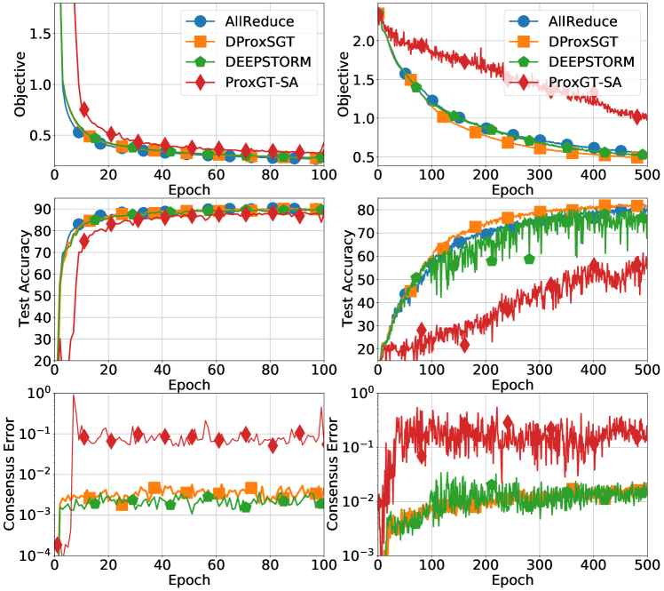
Figure 1: Results of training sparse neural networks by non-compressed methods with $r({\mathbf{x}})=\mu\|{\mathbf{x}}\|_{1}$ for the same number of epochs. Left: LeNet5 on FashionMNIST with $\mu=10^{-4}$. Right: FixupResnet20 on Cifar10 with $\mu=5\times 10^{-5}$.

The results for all methods are plotted in Figure 1. For LeNet5, DProxSGT produces almost the same curves as the centralized training method AllReduce, while on FixupResnet20, DProxSGT even outperforms AllReduce in terms of testing accuracy. This could be because AllReduce aggregates stochastic gradients from all the workers for each update and thus equivalently, it actually uses a larger batchsize. DEEPSTORM performs equally well as our method DProxSGT on training LeNet5. However, it gives lower testing accuracy than DProxSGT and also oscillates significantly more seriously on training the more complex neural network FixupResnet20. This appears to be caused by the momentum variance reduction scheme used in DEEPSTORM. In addition, we see that the large-batch training method ProxGT-SA performs much worse than DProxSGT within the same number of epochs (i.e., data pass), especially on training FixupResnet20.

5.2 Neural Network Training by Compressed Methods

In this subsection, we compare CDProxSGT with two state-of-the-art compressed training methods: Choco-SGD (Koloskova et al., 2019b, a) and BEER (Zhao et al., 2022). As Choco-SGD and BEER are studied only for problems without a regularizer, we set $r({\mathbf{x}})=0$ in (2) for the tests. Again, we compare their performance on training LeNet5 and FixupResnet20. The two non-compressed methods AllReduce and DProxSGT are included as baselines. The same compressors are used for CDProxSGT, Choco-SGD, and BEER, when compression is applied.

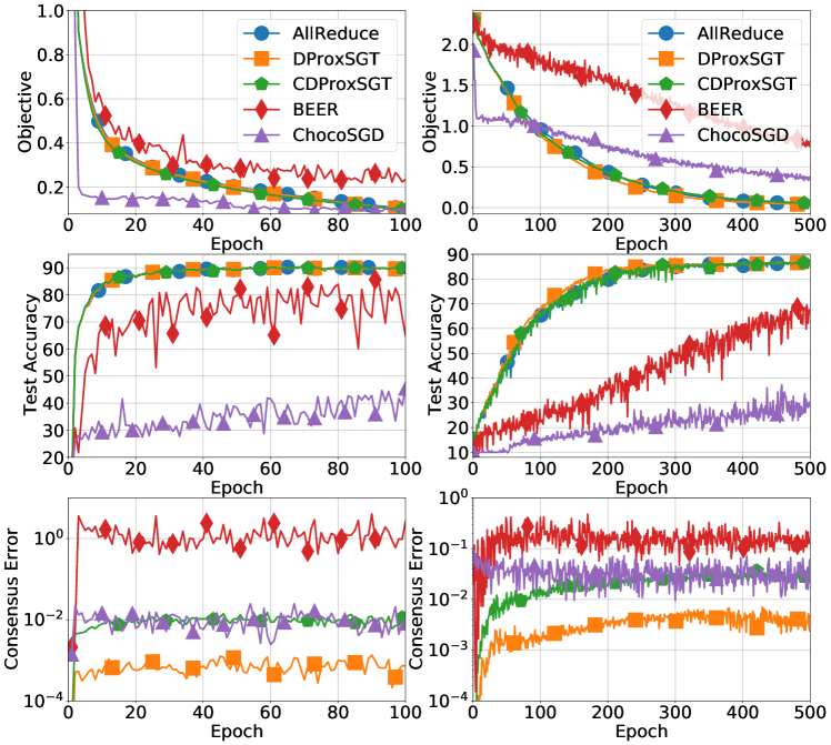
Figure 2: Results of training neural network models by compressed methods for the same number of epochs. Left: LeNet5 on FashionMNIST. Right: FixupResnet20 on Cifar10.

We run each method to 100 epochs for training LeNet5 on FashionMNIST. The compressors $Q_{y}$ and $Q_{x}$ are set to top-$k(0.3)$ (Aji & Heafield, 2017), i.e., taking the largest $30\%$ elements of an input vector in absolute values and zeroing out all others. We set batchsize to 8 and tune the learning rate $\eta$ to $0.01$ for AllReduce, DProxSGT, CDProxSGT and Choco-SGD, and for CDProxSGT, we set $\gamma_{x}=\gamma_{y}=0.5$. BEER is a large-batch training method. It uses a larger batchsize 256 and accordingly a larger learning rate $\eta=0.3$, which appears to be the best among $\{0.1,0.2,0.3,0.4\}$.

For training FixupResnet20 on the Cifar10 dataset, we run each method to 500 epochs. We take top-$k(0.4)$ (Aji & Heafield, 2017) as the compressors $Q_{y}$ and $Q_{x}$ and set $\gamma_{x}=\gamma_{y}=0.8$. For AllReduce, DProxSGT, CDProxSGT and Choco-SGD, we set their batchsize to 64 and tune the learning rate $\eta$ to $0.02$. For BEER, we use a larger batchsize 512 and a larger learning rate $\eta=0.1$, which is the best among $\{0.05,0.1,0.2,0.3\}$.

The results are shown in Figure 2. For both models, CDProxSGT yields almost the same curves of objective values and testing accuracy as its non-compressed counterpart DProxSGT and the centralized non-compressed method AllReduce. This indicates about 70% saving of communication for the training of LeNet5 and 60% saving for FixupResnet20 without sacrifying the testing accuracy. In comparison, BEER performs significantly worse than the proposed method CDProxSGT within the same number of epochs in terms of all the three measures, especially on training the more complex neural network FixupResnet20, which should be attributed to the use of a larger batch by BEER. Choco-SGD can produce comparable objective values. However, its testing accuracy is much lower than that produced by our method CDProxSGT. This should be because of the data heterogeneity that ChocoSGD cannot handle, while CDProxSGT applies the gradient tracking to successfully address the challenges of data heterogeneity.

6 Conclusion

We have proposed two decentralized proximal stochastic gradient methods, DProxSGT and CDProxSGT, for nonconvex composite problems with data heterogeneously distributed on the computing nodes of a connected graph. CDProxSGT is an extension of DProxSGT by applying compressions on the communicated model parameter and gradient information. Both methods need only a single or $\mathcal{O}(1)$ samples for each update, which is important to yield good generalization performance on training deep neural networks. The gradient tracking is used in both methods to address data heterogeneity. An $\mathcal{O}\left(\frac{1}{\epsilon^{4}}\right)$ sample complexity and communication complexity is established to both methods to produce an expected $\epsilon$-stationary solution. Numerical experiments on training neural networks demonstrate the good generalization performance and the ability of the proposed methods on handling heterogeneous data.

Appendix A Some Key Existing Lemmas

For $L$-smoothness function $f_{i}$, it holds for any ${\mathbf{x}},{\mathbf{y}}\in{\mathrm{dom}}(r)$,

$$\textstyle\big{|}f_{i}({\mathbf{y}})-f_{i}({\mathbf{x}})-\langle\nabla f_{i}({\mathbf{x}}),{\mathbf{y}}-{\mathbf{x}}\rangle\big{|}\leq\frac{L}{2}\|{\mathbf{y}}-{\mathbf{x}}\|^{2}.$$ (15)

From the smoothness of $f_{i}$ in Assumption 1, it follows that $f=\frac{1}{n}f_{i}$ is also $L$-smooth in ${\mathrm{dom}}(r)$.

When $f_{i}$ is $L$-smooth in ${\mathrm{dom}}(r)$, we have that $f_{i}(\cdot)+\frac{L}{2}\|\cdot\|^{2}$ is convex. Since $r(\cdot)$ is convex, $\phi_{i}(\cdot)+\frac{L}{2}\|\cdot\|^{2}$ is convex, i.e., $\phi_{i}$ is $L$-weakly convex for each $i$. So is $\phi$. In the following, we give some lemmas about weakly convex functions.

The following result is from Lemma II.1 in (Chen et al., 2021).

Lemma 8.

For any function $\psi$ on $\mathbb{R}^{d}$, if it is $L$-weakly convex, i.e., $\psi(\cdot)+\frac{L}{2}\|\cdot\|^{2}$ is convex, then for any ${\mathbf{x}}_{1},{\mathbf{x}}_{2},\ldots,{\mathbf{x}}_{m}\in\mathbb{R}^{d}$, it holds that

$$\psi\left(\sum_{i=1}^{m}a_{i}{\mathbf{x}}_{i}\right)\leq\sum_{i=1}^{m}a_{i}\psi({\mathbf{x}}_{i})+\frac{L}{2}\sum_{i=1}^{m-1}\sum_{j=i+1}^{m}a_{i}a_{j}\|{\mathbf{x}}_{i}-{\mathbf{x}}_{j}\|^{2},$$

where $a_{i}\geq 0$ for all $i$ and $\sum_{i=1}^{m}a_{i}=1$.

The first result below is from Lemma II.8 in (Chen et al., 2021), and the nonexpansiveness of the proximal mapping of a closed convex function is well known.

Lemma 9.

For any function $\psi$ on $\mathbb{R}^{d}$, if it is $L$-weakly convex, i.e., $\psi(\cdot)+\frac{L}{2}\|\cdot\|^{2}$ is convex, then the proximal mapping with $\lambda<\frac{1}{L}$ satisfies

$$\|{\mathbf{Prox}}_{\lambda\psi}({\mathbf{x}}_{1})-{\mathbf{Prox}}_{\lambda\psi}({\mathbf{x}}_{2})\|\leq\frac{1}{1-\lambda L}\|{\mathbf{x}}_{1}-{\mathbf{x}}_{2}\|.$$

For a closed convex function $r(\cdot)$, its proximal mapping is nonexpansive, i.e.,

$$\|{\mathbf{Prox}}_{r}({\mathbf{x}}_{1})-{\mathbf{Prox}}_{r}({\mathbf{x}}_{2})\|\leq\|{\mathbf{x}}_{1}-{\mathbf{x}}_{2}\|.$$

Lemma 10.

For $\mathrm{DProxSGT}$ in Algorithm 1 and $\mathrm{CDProxSGT}$ in Algorithm 2, we both have

$$\bar{\mathbf{y}}^{t}=\overline{\nabla}\mathbf{F}^{t},\quad\bar{\mathbf{x}}^{t}=\bar{\mathbf{x}}^{t+\frac{1}{2}}=\frac{1}{n}\sum_{i=1}^{n}{\mathbf{Prox}}_{\eta r}\left({\mathbf{x}}_{i}^{t}-\eta{\mathbf{y}}_{i}^{t}\right).$$ (16)

Proof.

For DProxSGT in Algorithm 1, taking the average among the workers on (3) to (6) gives

$$\bar{\mathbf{y}}^{t-\frac{1}{2}}=\bar{\mathbf{y}}^{t-1}+\overline{\nabla}\mathbf{F}^{t}-\overline{\nabla}\mathbf{F}^{t-1},\quad\bar{\mathbf{y}}^{t}=\bar{\mathbf{y}}^{t-\frac{1}{2}},\quad\bar{\mathbf{x}}^{t+\frac{1}{2}}=\frac{1}{n}\sum_{i=1}^{n}{\mathbf{Prox}}_{\eta r}\left({\mathbf{x}}_{i}^{t}-\eta{\mathbf{y}}_{i}^{t}\right),\quad\bar{\mathbf{x}}^{t}=\bar{\mathbf{x}}^{t+\frac{1}{2}},$$ (17)

where $\mathbf{1}^{\top}\mathbf{W}=\mathbf{1}^{\top}$ follows from Assumption 2. With $\bar{\mathbf{y}}^{-1}=\overline{\nabla}\mathbf{F}^{-1}$, we have (16).

Similarly, for CDProxSGT in Algorithm 2, taking the average on (44) to (49) will also give (17) and (16). ∎

In the rest of the analysis, we define the Moreau envelope of $\phi$ for $\lambda\in(0,\frac{1}{L})$ as

$$\phi_{\lambda}({\mathbf{x}})=\min_{\mathbf{y}}\left\{\phi({\mathbf{y}})+\frac{1}{2\lambda}\|{\mathbf{y}}-{\mathbf{x}}\|^{2}\right\}.$$

Denote the minimizer as

$${\mathbf{Prox}}_{\lambda\phi}({\mathbf{x}}):=\operatorname*{arg\,min}_{{\mathbf{y}}}\phi({\mathbf{y}})+\frac{1}{2\lambda}\|{\mathbf{y}}-{\mathbf{x}}\|^{2}.$$

In addition, we will use the notation $\widehat{{\mathbf{x}}}^{t}_{i}$ and $\widehat{{\mathbf{x}}}^{t+\frac{1}{2}}_{i}$ that are defined by

$$\widehat{{\mathbf{x}}}^{t}_{i}={\mathbf{Prox}}_{\lambda\phi}({\mathbf{x}}^{t}_{i}),\ \widehat{{\mathbf{x}}}^{t+\frac{1}{2}}_{i}={\mathbf{Prox}}_{\lambda\phi}({\mathbf{x}}^{t+\frac{1}{2}}_{i}),\,\forall\,i\in\mathcal{N},$$ (18)

where $\lambda\in(0,\frac{1}{L})$.

Appendix B Convergence Analysis for DProxSGT

In this section, we analyze the convergence rate of DProxSGT in Algorithm 1. For better readability, we use the matrix form of Algorithm 1. By the notation introduced in section 1.2, we can write (3)-(6) in the more compact matrix form:

$$\mathbf{Y}^{t-\frac{1}{2}}=\mathbf{Y}^{t-1}+\nabla\mathbf{F}^{t}-\nabla\mathbf{F}^{t-1},$$ (19)

$$\mathbf{Y}^{t}=\mathbf{Y}^{t-\frac{1}{2}}\mathbf{W},$$ (20)

$$\mathbf{X}^{t+\frac{1}{2}}={\mathbf{Prox}}_{\eta r}\left(\mathbf{X}^{t}-\eta\mathbf{Y}^{t}\right)\triangleq[{\mathbf{Prox}}_{\eta r}\left({\mathbf{x}}_{1}^{t}-\eta{\mathbf{y}}_{1}^{t}\right),\ldots,{\mathbf{Prox}}_{\eta r}\left({\mathbf{x}}_{n}^{t}-\eta{\mathbf{y}}_{n}^{t}\right)],$$ (21)

$$\mathbf{X}^{t+1}=\mathbf{X}^{t+\frac{1}{2}}\mathbf{W}.$$ (22)

Below, we first bound $\|\widehat{\mathbf{X}}^{t}-\mathbf{X}^{t+\frac{1}{2}}\|^{2}$ in Lemma 11. Then we give the bounds of the consensus error $\|\mathbf{X}_{\perp}^{t}\|$ and $\|\mathbf{Y}_{\perp}^{t}\|$ and $\phi_{\lambda}({\mathbf{x}}_{i}^{t+1})$ after one step in Lemmas 12, 13, and 14. Finally, we prove Theorem 4 by constructing a Lyapunov function that involves $\|\mathbf{X}_{\perp}^{t}\|$, $\|\mathbf{Y}_{\perp}^{t}\|$, and $\phi_{\lambda}({\mathbf{x}}_{i}^{t+1})$.

Lemma 11.

Let $\eta\leq\lambda\leq\frac{1}{4L}$. Then

$$\mathbb{E}\big{[}\|\widehat{\mathbf{X}}^{t}-\mathbf{X}^{t+\frac{1}{2}}\|^{2}\big{]}\leq ~{}4\mathbb{E}\big{[}\|\mathbf{X}^{t}_{\perp}\|^{2}\big{]}+\left(1-\frac{\eta}{2\lambda}\right)\mathbb{E}\big{[}\|\widehat{\mathbf{X}}^{t}-\mathbf{X}^{t}\|^{2}\big{]}+4\eta^{2}\mathbb{E}\big{[}\|\mathbf{Y}^{t}_{\perp}\|^{2}\big{]}+2\eta^{2}\sigma^{2}.$$ (23)

Proof.

By the definition of $\widehat{\mathbf{x}}^{t}_{i}$ in (18), we have $0\in\nabla f(\widehat{\mathbf{x}}^{t}_{i})+\partial r(\widehat{\mathbf{x}}^{t}_{i})+\frac{1}{\lambda}(\widehat{\mathbf{x}}^{t}_{i}-{\mathbf{x}}^{t}_{i})$, i.e.,

$$\textstyle 0\in\partial r(\widehat{\mathbf{x}}^{t}_{i})+\frac{1}{\eta}\left(\frac{\eta}{\lambda}\widehat{\mathbf{x}}^{t}_{i}-\frac{\eta}{\lambda}{\mathbf{x}}^{t}_{i}+\eta\nabla f(\widehat{\mathbf{x}}^{t}_{i})\right)=\partial r(\widehat{\mathbf{x}}^{t}_{i})+\frac{1}{\eta}\left(\widehat{\mathbf{x}}^{t}_{i}-\left(\frac{\eta}{\lambda}{\mathbf{x}}^{t}_{i}-\eta\nabla f(\widehat{\mathbf{x}}^{t}_{i})+\left(1-\frac{\eta}{\lambda}\right)\widehat{\mathbf{x}}^{t}_{i}\right)\right).$$

Thus we have $\widehat{\mathbf{x}}^{t}_{i}={\mathbf{Prox}}_{\eta r}\left(\frac{\eta}{\lambda}{\mathbf{x}}^{t}_{i}-\eta\nabla f(\widehat{\mathbf{x}}^{t}_{i})+\left(1-\frac{\eta}{\lambda}\right)\widehat{\mathbf{x}}^{t}_{i}\right)$. Then by (5), the convexity of $r$, and Lemma 9,

$$~{}\textstyle\|\widehat{\mathbf{x}}_{i}^{t}-{\mathbf{x}}_{i}^{t+\frac{1}{2}}\|^{2}=\left\|{\mathbf{Prox}}_{\eta r}\left(\frac{\eta}{\lambda}{\mathbf{x}}^{t}_{i}-\eta\nabla f(\widehat{\mathbf{x}}^{t}_{i})+\left(1-\frac{\eta}{\lambda}\right)\widehat{\mathbf{x}}^{t}_{i}\right)-{\mathbf{Prox}}_{\eta r}\left({\mathbf{x}}_{i}^{t}-\eta{\mathbf{y}}^{t}_{i}\right)\right\|^{2}$$

$$\leq ~{}\textstyle\left\|\frac{\eta}{\lambda}{\mathbf{x}}^{t}_{i}-\eta\nabla f(\widehat{\mathbf{x}}^{t}_{i})+\left(1-\frac{\eta}{\lambda}\right)\widehat{\mathbf{x}}^{t}_{i}-({\mathbf{x}}^{t}_{i}-\eta{\mathbf{y}}^{t}_{i})\right\|^{2}=\left\|\left(1-\frac{\eta}{\lambda}\right)(\widehat{\mathbf{x}}^{t}_{i}-{\mathbf{x}}^{t}_{i})-\eta(\nabla f(\widehat{\mathbf{x}}^{t}_{i})-{\mathbf{y}}^{t}_{i})\right\|^{2}$$

$$= ~{}\textstyle\left(1-\frac{\eta}{\lambda}\right)^{2}\left\|\widehat{\mathbf{x}}^{t}_{i}-{\mathbf{x}}^{t}_{i}\right\|^{2}+\eta^{2}\left\|{\mathbf{y}}^{t}_{i}-\nabla f(\widehat{\mathbf{x}}^{t}_{i})\right\|^{2}+2\left(1-\frac{\eta}{\lambda}\right)\eta\left\langle\widehat{\mathbf{x}}^{t}_{i}-{\mathbf{x}}_{i}^{t},{\mathbf{y}}_{i}^{t}-\nabla f({\mathbf{x}}^{t}_{i})+\nabla f({\mathbf{x}}^{t}_{i})-\nabla f(\widehat{\mathbf{x}}^{t}_{i})\right\rangle$$

$$\leq ~{}\textstyle\left(\left(1-\frac{\eta}{\lambda}\right)^{2}+2\left(1-\frac{\eta}{\lambda}\right)\eta L\right)\left\|\widehat{\mathbf{x}}^{t}_{i}-{\mathbf{x}}^{t}_{i}\right\|^{2}+\eta^{2}\left\|{\mathbf{y}}^{t}_{i}-\nabla f(\widehat{\mathbf{x}}^{t}_{i})\right\|^{2}+2\left(1-\frac{\eta}{\lambda}\right)\eta\left\langle\widehat{\mathbf{x}}^{t}_{i}-{\mathbf{x}}_{i}^{t},{\mathbf{y}}_{i}^{t}-\nabla f({\mathbf{x}}^{t}_{i})\right\rangle,$$ (24)

where the second inequality holds by $\left\langle\widehat{\mathbf{x}}^{t}_{i}-{\mathbf{x}}_{i}^{t},\nabla f({\mathbf{x}}^{t}_{i})-\nabla f(\widehat{\mathbf{x}}^{t}_{i})\right\rangle\leq L\left\|\widehat{\mathbf{x}}^{t}_{i}-{\mathbf{x}}_{i}^{t}\right\|^{2}$. The second term in the right hand side of (24) can be bounded by

$$~{}\textstyle\mathbb{E}_{t}[\|{\mathbf{y}}^{t}_{i}-\nabla f(\widehat{\mathbf{x}}^{t}_{i})\|^{2}\big{]}\overset{\eqref{eq:x_y_mean}}{=}\mathbb{E}_{t}\big{[}\|{\mathbf{y}}^{t}_{i}-\bar{\mathbf{y}}^{t}+\overline{\nabla}\mathbf{F}^{t}-\nabla f(\widehat{\mathbf{x}}^{t}_{i})\|^{2}\big{]}\leq 2\mathbb{E}_{t}\big{[}\|{\mathbf{y}}^{t}_{i}-\bar{\mathbf{y}}^{t}\|^{2}\big{]}+2\mathbb{E}_{t}\big{[}\big{\|}\overline{\nabla}\mathbf{F}^{t}-\nabla f(\widehat{\mathbf{x}}^{t}_{i})\big{\|}^{2}\big{]}$$

$$= ~{}2\mathbb{E}_{t}\big{[}\|{\mathbf{y}}^{t}_{i}-\bar{\mathbf{y}}^{t}\|^{2}\big{]}+2\mathbb{E}_{t}\big{[}\|\overline{\nabla}\mathbf{F}^{t}-\overline{\nabla}\mathbf{f}^{t}\|^{2}\big{]}+2\|\overline{\nabla}\mathbf{f}^{t}-\nabla f(\widehat{\mathbf{x}}^{t}_{i})\|^{2}$$

$$\leq ~{}2\mathbb{E}_{t}[\|{\mathbf{y}}_{i}^{t}-\bar{\mathbf{y}}^{t}\|^{2}\big{]}+\frac{2}{n^{2}}\sum_{j=1}^{n}\mathbb{E}_{t}\big{[}\|\nabla F_{j}({\mathbf{x}}_{j}^{t},\xi_{j}^{t})-\nabla f_{j}({\mathbf{x}}_{j}^{t})\|^{2}\big{]}+4\|\overline{\nabla}\mathbf{f}^{t}-\nabla f({\mathbf{x}}^{t}_{i})\|^{2}+4\|\nabla f({\mathbf{x}}^{t}_{i})-\nabla f(\widehat{\mathbf{x}}^{t}_{i})\|^{2}$$

$$\leq ~{}2\mathbb{E}_{t}[\|{\mathbf{y}}_{i}^{t}-\bar{\mathbf{y}}^{t}\|^{2}\big{]}+2\frac{\sigma^{2}}{n}+4\|\overline{\nabla}\mathbf{f}^{t}-\nabla f({\mathbf{x}}^{t}_{i})\|^{2}+4L^{2}\|{\mathbf{x}}^{t}_{i}-\widehat{\mathbf{x}}^{t}_{i}\|^{2},$$

where the second equality holds by the unbiasedness of stochastic gradients, and the second inequality holds also by the independence between $\xi_{i}^{t}$’s. In the last inequality, we use the bound of the variance of stochastic gradients, and the $L$-smooth assumption. Taking the full expectation over the above inequality and summing for all $i$ give

$$\sum_{i=1}^{n}\mathbb{E}\big{[}\|{\mathbf{y}}^{t}_{i}-\nabla f(\widehat{\mathbf{x}}^{t}_{i})\|^{2}]\leq 2\mathbb{E}\big{[}\|\mathbf{Y}^{t}_{\perp}\|^{2}]+2\sigma^{2}+8L^{2}\mathbb{E}\big{[}\|\mathbf{X}^{t}_{\perp}\|^{2}]+4L^{2}\mathbb{E}\big{[}\|\mathbf{X}^{t}-\widehat{\mathbf{X}}^{t}\|^{2}].$$ (25)

To have the inequality above, we have used

$$~{}\sum_{i=1}^{n}\left\|\overline{\nabla}\mathbf{f}^{t}-\nabla f({\mathbf{x}}^{t}_{i})\right\|^{2}\leq\frac{1}{n}\sum_{i=1}^{n}\sum_{j=1}^{n}\left\|\nabla f_{j}({\mathbf{x}}_{j}^{t})-\nabla f_{j}({\mathbf{x}}^{t}_{i})\right\|^{2}\leq\frac{L^{2}}{n}\sum_{i=1}^{n}\sum_{j=1}^{n}\left\|{\mathbf{x}}_{j}^{t}-{\mathbf{x}}^{t}_{i}\right\|^{2}$$

$$= ~{}\frac{L^{2}}{n}\sum_{i=1}^{n}\sum_{j=1}^{n}\left(\left\|{\mathbf{x}}_{j}^{t}-\bar{\mathbf{x}}^{t}\right\|^{2}+\left\|\bar{\mathbf{x}}^{t}-{\mathbf{x}}^{t}_{i}\right\|^{2}+2\left\langle{\mathbf{x}}_{j}^{t}-\bar{\mathbf{x}}^{t},\bar{\mathbf{x}}^{t}-{\mathbf{x}}^{t}_{i}\right\rangle\right)=2L^{2}\left\|\mathbf{X}^{t}_{\perp}\right\|^{2},$$ (26)

where the last equality holds by $\frac{1}{n}\sum_{i=1}^{n}\sum_{j=1}^{n}\left\langle{\mathbf{x}}_{j}^{t}-\bar{\mathbf{x}}^{t},\bar{\mathbf{x}}^{t}-{\mathbf{x}}^{t}_{i}\right\rangle=\sum_{i=1}^{n}\left\langle\frac{1}{n}\sum_{j=1}^{n}({\mathbf{x}}_{j}^{t}-\bar{\mathbf{x}}^{t}),\bar{\mathbf{x}}^{t}-{\mathbf{x}}^{t}_{i}\right\rangle=\sum_{i=1}^{n}\left\langle\bar{\mathbf{x}}^{t}-\bar{\mathbf{x}}^{t},\bar{\mathbf{x}}^{t}-{\mathbf{x}}^{t}_{i}\right\rangle=0$ from the definition of $\bar{\mathbf{x}}$.

About the third term in the right hand side of (24), we have

$$~{}\sum_{i=1}^{n}\mathbb{E}\left[\left\langle\widehat{\mathbf{x}}^{t}_{i}-{\mathbf{x}}_{i}^{t},{\mathbf{y}}_{i}^{t}-\nabla f({\mathbf{x}}^{t}_{i})\right\rangle\right]\overset{\eqref{eq:x_y_mean}}{=}\sum_{i=1}^{n}\mathbb{E}\left[\left\langle\widehat{\mathbf{x}}^{t}_{i}-{\mathbf{x}}_{i}^{t},{\mathbf{y}}_{i}^{t}-\bar{\mathbf{y}}^{t}+\overline{\nabla}\mathbf{F}^{t}-\nabla f({\mathbf{x}}^{t}_{i})\right\rangle\right]$$

$$= ~{}\textstyle\sum_{i=1}^{n}\mathbb{E}\big{[}\langle\widehat{\mathbf{x}}^{t}_{i}-\bar{\widehat{\mathbf{x}}}^{t},{\mathbf{y}}_{i}^{t}-\bar{\mathbf{y}}^{t}\rangle\big{]}+\sum_{i=1}^{n}\mathbb{E}\big{[}\langle\bar{{\mathbf{x}}}^{t}-{\mathbf{x}}_{i}^{t},{\mathbf{y}}_{i}^{t}-\bar{\mathbf{y}}^{t}\rangle\big{]}+\sum_{i=1}^{n}\mathbb{E}\left[\left\langle\widehat{\mathbf{x}}^{t}_{i}-{\mathbf{x}}_{i}^{t},\mathbb{E}_{t}\left[\overline{\nabla}\mathbf{F}^{t}\right]-\nabla f({\mathbf{x}}^{t}_{i})\right\rangle\right]$$

$$\leq ~{}\frac{1}{2\eta}\left(\textstyle\mathbb{E}\big{[}\|\widehat{\mathbf{X}}^{t}_{\perp}\|^{2}\big{]}+\mathbb{E}\big{[}\|\mathbf{X}^{t}_{\perp}\|^{2}\big{]}\right)+\eta\mathbb{E}\big{[}\|\mathbf{Y}^{t}_{\perp}\|^{2}\big{]}+\textstyle L\mathbb{E}\big{[}\|\widehat{\mathbf{X}}^{t}-\mathbf{X}^{t}\|^{2}\big{]}+\frac{1}{4L}\sum_{i=1}^{n}\mathbb{E}\big{[}\|\overline{\nabla}{\mathbf{f}}^{t}-\nabla f({\mathbf{x}}^{t}_{i})\|^{2}\big{]}$$

$$\leq ~{}\left(\textstyle\frac{1}{2\eta(1-\lambda L)^{2}}+\frac{1}{2\eta}+\frac{L}{2}\right)\mathbb{E}\big{[}\|\mathbf{X}^{t}_{\perp}\|^{2}\big{]}+\eta\mathbb{E}\big{[}\|\mathbf{Y}^{t}_{\perp}\|^{2}\big{]}+L\mathbb{E}\big{[}\|\widehat{\mathbf{X}}^{t}-\mathbf{X}^{t}\|^{2}\big{]},$$ (27)

where $\textstyle\sum_{i=1}^{n}\big{\langle}\bar{\widehat{\mathbf{x}}}^{t},{\mathbf{y}}_{i}^{t}-\bar{\mathbf{y}}^{t}\big{\rangle}=0$ and $\sum_{i=1}^{n}\left\langle\bar{{\mathbf{x}}}^{t},{\mathbf{y}}_{i}^{t}-\bar{\mathbf{y}}^{t}\right\rangle=0$ is used in the second equality, $\mathbb{E}_{t}\left[\overline{\nabla}\mathbf{F}^{t}\right]=\overline{\nabla}{\mathbf{f}}^{t}$ is used in the first inequality, and $\|\widehat{\mathbf{X}}^{t}_{\perp}\|^{2}=\left\|\left({\mathbf{Prox}}_{\lambda\phi}(\mathbf{X}^{t})-{\mathbf{Prox}}_{\lambda\phi}(\bar{\mathbf{x}}^{t})\mathbf{1}^{\top}\right)(\mathbf{I}-\mathbf{J})\right\|^{2}\leq\frac{1}{(1-\lambda L)^{2}}\|\mathbf{X}^{t}-\bar{\mathbf{X}}^{t}\|^{2}$ and (26) are used in the last inequality.

Now we can bound the summation of (24) by using (25) and (27):

$$~{}\mathbb{E}\big{[}\|\widehat{\mathbf{X}}^{t}-\mathbf{X}^{t+\frac{1}{2}}\|^{2}\big{]}$$

$$\leq ~{}\left(\textstyle\left(1-\frac{\eta}{\lambda}\right)^{2}+2\left(1-\frac{\eta}{\lambda}\right)\eta L\right)\mathbb{E}\big{[}\|\widehat{\mathbf{X}}^{t}-\mathbf{X}^{t}\|^{2}\big{]}$$

$$~{}+\eta^{2}\left(2\mathbb{E}[\|\mathbf{Y}^{t}_{\perp}\|^{2}\big{]}+2\sigma^{2}+8L^{2}\mathbb{E}\big{[}\|\mathbf{X}^{t}_{\perp}\|^{2}\big{]}+4L^{2}\mathbb{E}\big{[}\|\mathbf{X}^{t}-\widehat{\mathbf{X}}^{t}\|^{2}\big{]}\right)$$

$$~{}+\textstyle 2\left(1-\frac{\eta}{\lambda}\right)\eta\left(\textstyle\left(\frac{1}{2\eta(1-\lambda L)^{2}}+\frac{1}{2\eta}+\frac{L}{2}\right)\mathbb{E}\big{[}\|\mathbf{X}^{t}_{\perp}\|^{2}\big{]}+\eta\mathbb{E}\big{[}\|\mathbf{Y}^{t}_{\perp}\|^{2}\big{]}+L\mathbb{E}\big{[}\|\widehat{\mathbf{X}}^{t}-\mathbf{X}^{t}\|^{2}\big{]}\right)$$

$$= ~{}\textstyle\left(1-2\eta(\frac{1}{\lambda}-2L)+\frac{\eta^{2}}{\lambda}(\frac{1}{\lambda}-2L)+2L\eta^{2}(-\frac{1}{\lambda}+2L)\right)\mathbb{E}\big{[}\|\widehat{\mathbf{X}}^{t}-\mathbf{X}^{t}\|^{2}\big{]}+2\eta^{2}\sigma^{2}$$

$$~{}+\textstyle\left(\left(1-\frac{\eta}{\lambda}\right)(1+\frac{1}{(1-\lambda L)^{2}}+\eta L)+8\eta^{2}L^{2}\right)\mathbb{E}\big{[}\|\mathbf{X}^{t}_{\perp}\|^{2}\big{]}+2(2-\frac{\eta}{\lambda})\eta^{2}\mathbb{E}\big{[}\|\mathbf{Y}^{t}_{\perp}\|^{2}\big{]}.$$

With $\eta\leq\lambda\leq\frac{1}{4L}$, we have $\frac{1}{(1-\lambda L)^{2}}\leq 2$ and (23) follows from the inequality above.

∎

Lemma 12.

The consensus error of $\mathbf{X}$ satisfies the following inequality

$$\mathbb{E}\big{[}\|\mathbf{X}^{t}_{\perp}\|^{2}\big{]}\leq\frac{1+\rho^{2}}{2}\mathbb{E}\big{[}\|\mathbf{X}^{t-1}_{\perp}\|^{2}\big{]}+\frac{2\rho^{2}\eta^{2}}{1-\rho^{2}}\mathbb{E}\big{[}\|\mathbf{Y}^{t-1}_{\perp}\|^{2}\big{]}.$$ (28)

Proof.

With the updates (5) and (6), we have

$$~{}\mathbb{E}\big{[}\|\mathbf{X}^{t}_{\perp}\|^{2}\big{]}=\mathbb{E}\big{[}\|\mathbf{X}^{t-\frac{1}{2}}\mathbf{W}(\mathbf{I}-\mathbf{J})\|^{2}\big{]}=\mathbb{E}\big{[}\|\mathbf{X}^{t-\frac{1}{2}}(\mathbf{W}-\mathbf{J})\|^{2}\big{]}$$

$$= ~{}\mathbb{E}\big{[}\|{\mathbf{Prox}}_{\eta r}\left(\mathbf{X}^{t-1}-\eta\mathbf{Y}^{t-1}\right)(\mathbf{W}-\mathbf{J})\|^{2}\big{]}$$

$$= ~{}\mathbb{E}\big{[}\|\left({\mathbf{Prox}}_{\eta r}\left(\mathbf{X}^{t-1}-\eta\mathbf{Y}^{t-1}\right)-{\mathbf{Prox}}_{\eta r}\left(\bar{\mathbf{x}}^{t-1}-\eta\bar{\mathbf{y}}^{t-1}\right)\mathbf{1}^{\top}\right)(\mathbf{W}-\mathbf{J})\|^{2}\big{]}$$

$$\leq ~{}\mathbb{E}\big{[}\|{\mathbf{Prox}}_{\eta r}\left(\mathbf{X}^{t-1}-\eta\mathbf{Y}^{t-1}\right)-{\mathbf{Prox}}_{\eta r}\left(\bar{\mathbf{x}}^{t-1}-\eta\bar{\mathbf{y}}^{t-1}\right)\mathbf{1}^{\top}\|^{2}\|(\mathbf{W}-\mathbf{J})\|^{2}_{2}]$$

$$\leq ~{}\rho^{2}\mathbb{E}\left[\textstyle\sum_{i=1}^{n}\|{\mathbf{Prox}}_{\eta r}\left({\mathbf{x}}_{i}^{t-1}-\eta{\mathbf{y}}_{i}^{t-1}\right)-{\mathbf{Prox}}_{\eta r}\left(\bar{\mathbf{x}}^{t-1}-\eta\bar{\mathbf{y}}^{t-1}\right)\|^{2}\right]$$

$$\leq ~{}\rho^{2}\mathbb{E}\left[\textstyle\sum_{i=1}^{n}\|\left({\mathbf{x}}_{i}^{t-1}-\eta{\mathbf{y}}_{i}^{t-1}\right)-\left(\bar{\mathbf{x}}^{t-1}-\eta\bar{\mathbf{y}}^{t-1}\right)\|^{2}\right]=\rho^{2}\mathbb{E}\big{[}\|\mathbf{X}^{t-1}_{\perp}-\eta\mathbf{Y}^{t-1}_{\perp}\|^{2}\big{]}$$

$$\leq ~{}\textstyle\big{(}\textstyle\rho^{2}+\frac{1-\rho^{2}}{2}\big{)}\mathbb{E}\big{[}\|\mathbf{X}^{t-1}_{\perp}\|^{2}\big{]}+\big{(}\textstyle\rho^{2}+\frac{2\rho^{4}}{1-\rho^{2}}\big{)}\eta^{2}\mathbb{E}\big{[}\|\mathbf{Y}^{t-1}_{\perp}\|^{2}\big{]}$$

$$= ~{}\textstyle\frac{1+\rho^{2}}{2}\mathbb{E}\big{[}\|\mathbf{X}^{t-1}_{\perp}\|^{2}\big{]}+\frac{1+\rho^{2}}{1-\rho^{2}}\rho^{2}\eta^{2}\mathbb{E}\big{[}\|\mathbf{Y}^{t-1}_{\perp}\|^{2}\big{]}$$

$$\leq ~{}\textstyle\frac{1+\rho^{2}}{2}\mathbb{E}\big{[}\|\mathbf{X}^{t-1}_{\perp}\|^{2}\big{]}+\frac{2\rho^{2}\eta^{2}}{1-\rho^{2}}\mathbb{E}\big{[}\|\mathbf{Y}^{t-1}_{\perp}\|^{2}\big{]},$$

where we have used $\mathbf{1}^{\top}(\mathbf{W}-\mathbf{J})=\mathbf{0}$ in the third equality, $\|\mathbf{W}-\mathbf{J}\|_{2}\leq\rho$ in the second inequality, and Lemma 9 in the third inequality, and $\rho\leq 1$ is used in the last inequality. ∎

Lemma 13.

Let $\eta\leq\min\{\lambda,\frac{1-\rho^{2}}{4\sqrt{6}\rho L}\}$ and $\lambda\leq\frac{1}{4L}$. The consensus error of $\mathbf{Y}$ satisfies

$$\mathbb{E}\big{[}\|\mathbf{Y}^{t}_{\perp}\|^{2}\big{]}\leq ~{}\frac{48\rho^{2}L^{2}}{1-\rho^{2}}\mathbb{E}\big{[}\|\mathbf{X}^{t-1}_{\perp}\|^{2}\big{]}\!+\!\frac{3\!+\!\rho^{2}}{4}\mathbb{E}\big{[}\|\mathbf{Y}^{t-1}_{\perp}\|^{2}\big{]}\!+\!\frac{12\rho^{2}L^{2}}{1-\rho^{2}}\mathbb{E}\big{[}\|\widehat{\mathbf{X}}^{t-1}-\mathbf{X}^{t-1}\|^{2}\big{]}\!+\!6n\sigma^{2}.$$ (29)

Proof.

By the updates (3) and (4), we have

$$~{}\mathbb{E}\big{[}\|\mathbf{Y}^{t}_{\perp}\|^{2}\big{]}=\mathbb{E}\big{[}\|\mathbf{Y}^{t-\frac{1}{2}}(\mathbf{W}-\mathbf{J})\|^{2}\big{]}=\mathbb{E}\big{[}\|\mathbf{Y}^{t-1}(\mathbf{W}-\mathbf{J})+(\nabla\mathbf{F}^{t}-\nabla\mathbf{F}^{t-1})(\mathbf{W}-\mathbf{J})\|^{2}\big{]}$$

$$= ~{}\mathbb{E}\big{[}\|\mathbf{Y}^{t-1}(\mathbf{I}-\mathbf{J})(\mathbf{W}-\mathbf{J})\|^{2}\big{]}+\mathbb{E}\big{[}\|(\nabla\mathbf{F}^{t}-\nabla\mathbf{F}^{t-1})(\mathbf{W}-\mathbf{J})\|^{2}\big{]}+2\mathbb{E}\big{[}\langle\mathbf{Y}^{t-1}(\mathbf{W}-\mathbf{J}),(\nabla\mathbf{F}^{t}-\nabla\mathbf{F}^{t-1})(\mathbf{W}-\mathbf{J})\rangle\big{]}$$

$$\leq ~{}\rho^{2}\mathbb{E}\big{[}\|\mathbf{Y}^{t-1}_{\perp}\|^{2}\big{]}+\rho^{2}\mathbb{E}\big{[}\|\nabla\mathbf{F}^{t}-\nabla\mathbf{F}^{t-1}\|^{2}\big{]}+2\mathbb{E}\big{[}\langle\mathbf{Y}^{t-1}(\mathbf{W}-\mathbf{J}),(\nabla\mathbf{f}^{t}-\nabla\mathbf{F}^{t-1})(\mathbf{W}-\mathbf{J})\rangle\big{]},$$ (30)

where we have used $\mathbf{J}\mathbf{W}=\mathbf{J}\mathbf{J}=\mathbf{J}$, $\|\mathbf{W}-\mathbf{J}\|_{2}\leq\rho$ and $\mathbb{E}_{t}[\nabla\mathbf{F}^{t}]=\nabla{\mathbf{f}}^{t}$. For the second term on the right hand side of (30), we have

$$~{}\mathbb{E}\big{[}\|\nabla\mathbf{F}^{t}-\nabla\mathbf{F}^{t-1}\|^{2}\big{]}=\mathbb{E}\big{[}\|\nabla\mathbf{F}^{t}-\nabla\mathbf{f}^{t}+\nabla\mathbf{f}^{t}-\nabla\mathbf{F}^{t-1}\|^{2}\big{]}$$

$$\overset{\mathbb{E}_{t}[\nabla\mathbf{F}^{t}]=\nabla\mathbf{f}^{t}}{=} ~{}\mathbb{E}\big{[}\|\nabla\mathbf{F}^{t}-\nabla\mathbf{f}^{t}\|^{2}\big{]}+\mathbb{E}\big{[}\|\nabla\mathbf{f}^{t}-\nabla\mathbf{f}^{t-1}+\nabla\mathbf{f}^{t-1}-\nabla\mathbf{F}^{t-1}\|^{2}\big{]}$$

$$\leq ~{}\mathbb{E}\big{[}\|\nabla\mathbf{F}^{t}-\nabla\mathbf{f}^{t}\|^{2}\big{]}+2\mathbb{E}\big{[}\|\nabla\mathbf{f}^{t}-\nabla\mathbf{f}^{t-1}\|^{2}\big{]}+2\mathbb{E}\big{[}\|\nabla\mathbf{f}^{t-1}-\nabla\mathbf{F}^{t-1}\|^{2}\big{]}$$

$$\leq ~{}3n\sigma^{2}+2L^{2}\mathbb{E}\big{[}\|\mathbf{X}^{t}-\mathbf{X}^{t-1}\|^{2}\big{]}.$$ (31)

For the third term on the right hand side of (30), we have

$$~{}2\mathbb{E}\big{[}\langle\mathbf{Y}^{t-1}(\mathbf{W}-\mathbf{J}),(\nabla\mathbf{f}^{t}-\nabla\mathbf{F}^{t-1})(\mathbf{W}-\mathbf{J})\rangle\big{]}$$

$$= ~{}2\mathbb{E}\big{[}\langle\mathbf{Y}^{t-1}(\mathbf{W}-\mathbf{J}),(\nabla\mathbf{f}^{t}-\nabla\mathbf{f}^{t-1})(\mathbf{W}-\mathbf{J})\rangle\big{]}+2\mathbb{E}\big{[}\langle\mathbf{Y}^{t-1}(\mathbf{W}-\mathbf{J}),(\nabla\mathbf{f}^{t-1}-\nabla\mathbf{F}^{t-1})(\mathbf{W}-\mathbf{J})\rangle\big{]}$$

$$= ~{}2\mathbb{E}\big{[}\langle\mathbf{Y}^{t-1}(\mathbf{I}-\mathbf{J})(\mathbf{W}-\mathbf{J}),(\nabla\mathbf{f}^{t}-\nabla\mathbf{f}^{t-1})(\mathbf{W}-\mathbf{J})\rangle\big{]}$$

$$~{}+2\mathbb{E}\big{[}\langle(\mathbf{Y}^{t-2}+\nabla\mathbf{F}^{t-1}-\nabla\mathbf{F}^{t-2})\mathbf{W}(\mathbf{W}-\mathbf{J}),(\nabla\mathbf{f}^{t-1}-\nabla\mathbf{F}^{t-1})(\mathbf{W}-\mathbf{J})\rangle\big{]}$$

$$= ~{}2\mathbb{E}\big{[}\langle\mathbf{Y}^{t-1}(\mathbf{I}-\mathbf{J})(\mathbf{W}-\mathbf{J}),(\nabla\mathbf{f}^{t}-\nabla\mathbf{f}^{t-1})(\mathbf{W}-\mathbf{J})\rangle\big{]}$$

$$~{}+2\mathbb{E}\big{[}\langle(\nabla\mathbf{F}^{t-1}-\nabla\mathbf{f}^{t-1})\mathbf{W}(\mathbf{W}-\mathbf{J}),(\nabla\mathbf{f}^{t-1}-\nabla\mathbf{F}^{t-1})(\mathbf{W}-\mathbf{J})\rangle\big{]}$$

$$\leq ~{}2\mathbb{E}\big{[}\|\mathbf{Y}^{t-1}(\mathbf{I}-\mathbf{J})(\mathbf{W}-\mathbf{J})\|\cdot\|(\nabla\mathbf{f}^{t}-\nabla\mathbf{f}^{t-1})(\mathbf{W}-\mathbf{J})\|\big{]}$$

$$~{}+2\mathbb{E}\big{[}\|(\nabla\mathbf{F}^{t-1}-\nabla\mathbf{f}^{t-1})\mathbf{W}(\mathbf{W}-\mathbf{J})\|\cdot\|(\nabla\mathbf{f}^{t-1}-\nabla\mathbf{F}^{t-1})(\mathbf{W}-\mathbf{J})\|\big{]}$$

$$\leq ~{}2\rho^{2}\mathbb{E}\big{[}\|\mathbf{Y}^{t-1}_{\perp}\|\cdot\|\nabla\mathbf{f}^{t}-\nabla\mathbf{f}^{t-1}\|\big{]}+2\rho^{2}\mathbb{E}\big{[}\|\nabla\mathbf{F}^{t-1}-\nabla\mathbf{f}^{t-1}\|^{2}\big{]}$$

$$\leq ~{}\textstyle\frac{1-\rho^{2}}{2}\mathbb{E}\big{[}\|\mathbf{Y}^{t-1}_{\perp}\|^{2}\big{]}+\frac{2\rho^{4}}{1-\rho^{2}}\mathbb{E}\big{[}\|\nabla\mathbf{f}^{t}-\nabla\mathbf{f}^{t-1}\|^{2}\big{]}+2\rho^{2}n\sigma^{2}$$

$$\leq ~{}\textstyle\frac{1-\rho^{2}}{2}\mathbb{E}\big{[}\|\mathbf{Y}^{t-1}_{\perp}\|^{2}\big{]}+\frac{2\rho^{4}L^{2}}{1-\rho^{2}}\mathbb{E}\big{[}\|\mathbf{X}^{t}-\mathbf{X}^{t-1}\|^{2}\big{]}+2\rho^{2}n\sigma^{2},$$ (32)

where the second equality holds by $\mathbf{W}-\mathbf{J}=(\mathbf{I}-\mathbf{J})(\mathbf{W}-\mathbf{J})$, (3) and (4), the third equality holds because $\mathbf{Y}^{t-2}-\nabla\mathbf{F}^{t-2}-\nabla\mathbf{f}^{t-1}$ does not depend on $\xi_{i}^{t-1}$’s, and the second inequality holds because $\|\mathbf{W}-\mathbf{J}\|_{2}\leq\rho$ and $\|\mathbf{W}\|_{2}\leq 1$. Plugging (31) and (32) into (30), we have

$$\mathbb{E}\big{[}\|\mathbf{Y}^{t}_{\perp}\|^{2}\big{]}\leq ~{}\textstyle\frac{1+\rho^{2}}{2}\mathbb{E}\big{[}\|\mathbf{Y}^{t-1}_{\perp}\|^{2}\big{]}+\frac{2\rho^{2}L^{2}}{1-\rho^{2}}\mathbb{E}\big{[}\|\mathbf{X}^{t}-\mathbf{X}^{t-1}\|^{2}\big{]}+5\rho^{2}n\sigma^{2},$$ (33)

where we have used $1+\frac{\rho^{2}}{1-\rho^{2}}=\frac{1}{1-\rho^{2}}$. For the second term in the right hand side of (33), we have

$$~{}\|\mathbf{X}^{t+1}-\mathbf{X}^{t}\|^{2}=\|\mathbf{X}^{t+\frac{1}{2}}\mathbf{W}-\mathbf{X}^{t}\|^{2}=\|(\mathbf{X}^{t+\frac{1}{2}}-\widehat{\mathbf{X}}^{t})\mathbf{W}+(\widehat{\mathbf{X}}^{t}-\mathbf{X}^{t})\mathbf{W}+\mathbf{X}^{t}(\mathbf{W}-\mathbf{I})\|^{2}$$

$$\leq ~{}3\|(\mathbf{X}^{t+\frac{1}{2}}-\widehat{\mathbf{X}}^{t})\mathbf{W}\|^{2}+3\|(\widehat{\mathbf{X}}^{t}-\mathbf{X}^{t})\mathbf{W}\|^{2}+3\|\mathbf{X}^{t}(\mathbf{I}-\mathbf{J})(\mathbf{W}-\mathbf{I})\|^{2}$$

$$\leq ~{}3\|\mathbf{X}^{t+\frac{1}{2}}-\widehat{\mathbf{X}}^{t}\|^{2}+3\|\widehat{\mathbf{X}}^{t}-\mathbf{X}^{t}\|^{2}+12\|\mathbf{X}^{t}_{\perp}\|^{2},$$ (34)

where in the first inequality we have used $\mathbf{X}^{t}(\mathbf{W}-\mathbf{I})=\mathbf{X}^{t}(\mathbf{I}-\mathbf{J})(\mathbf{W}-\mathbf{I})$ from $\mathbf{J}(\mathbf{W}-\mathbf{I})=\mathbf{J}-\mathbf{J}$, and in the second inequality we have used $\|\mathbf{W}\|_{2}\leq 1$ and $\|\mathbf{W}-\mathbf{I}\|_{2}\leq 2$.

Taking expectation over both sides of (34) and using (23), we have

$$~{}\mathbb{E}\big{[}\|\mathbf{X}^{t+1}-\mathbf{X}^{t}\|^{2}\big{]}$$

$$\leq ~{}3\left(\textstyle 4\mathbb{E}\big{[}\|\mathbf{X}^{t}_{\perp}\|^{2}\big{]}+\left(1-\frac{\eta}{2\lambda}\right)\mathbb{E}\big{[}\|\widehat{\mathbf{X}}^{t}-\mathbf{X}^{t}\|^{2}\big{]}+4\eta^{2}\mathbb{E}\big{[}\|\mathbf{Y}^{t}_{\perp}\|^{2}\big{]}+2\eta^{2}\sigma^{2}\right)+3\mathbb{E}\big{[}\|\widehat{\mathbf{X}}^{t}-\mathbf{X}^{t}\|^{2}\big{]}+12\mathbb{E}\big{[}\|\mathbf{X}^{t}_{\perp}\|^{2}\big{]}$$

$$= ~{}3\textstyle\left(2-\frac{\eta}{2\lambda}\right)\mathbb{E}\big{[}\|\widehat{\mathbf{X}}^{t}-\mathbf{X}^{t}\|^{2}\big{]}+12\eta^{2}\mathbb{E}\big{[}\|\mathbf{Y}^{t}_{\perp}\|^{2}\big{]}+6\eta^{2}\sigma^{2}+24\mathbb{E}\big{[}\|\mathbf{X}^{t}_{\perp}\|^{2}\big{]}.$$

Plugging the inequality above into (33) gives

$$\mathbb{E}\big{[}\|\mathbf{Y}^{t}_{\perp}\|^{2}\big{]}\leq ~{}\left(\textstyle\frac{1+\rho^{2}}{2}+\frac{24\rho^{2}L^{2}\eta^{2}}{1-\rho^{2}}\right)\mathbb{E}\big{[}\|\mathbf{Y}^{t-1}_{\perp}\|^{2}\big{]}+\textstyle 5\rho^{2}n\sigma^{2}+\frac{12\rho^{2}L^{2}\eta^{2}\sigma^{2}}{1-\rho^{2}}$$

$$~{}\textstyle+\frac{6\rho^{2}L^{2}}{1-\rho^{2}}\left(\textstyle 2-\frac{\eta}{2\lambda}\right)\mathbb{E}\big{[}\|\widehat{\mathbf{X}}^{t-1}-\mathbf{X}^{t-1}\|^{2}\big{]}+\frac{48\rho^{2}L^{2}}{1-\rho^{2}}\mathbb{E}\big{[}\|\mathbf{X}^{t-1}_{\perp}\|^{2}\big{]}.$$

By $\rho<1$ and $\eta\leq\frac{1-\rho^{2}}{4\sqrt{6}\rho L}$, we have $\frac{24\rho^{2}L^{2}\eta^{2}}{1-\rho^{2}}\leq\frac{1-\rho^{2}}{4}$ and $\frac{12\rho^{2}L^{2}\eta^{2}}{1-\rho^{2}}\leq\frac{1-\rho^{2}}{8}\leq n$, and further (29). ∎

Lemma 14.

Let $\eta\leq\lambda\leq\frac{1}{4L}$. It holds

$$\sum_{i=1}^{n}\mathbb{E}[\phi_{\lambda}({\mathbf{x}}_{i}^{t+1})]\leq ~{}\sum_{i=1}^{n}\mathbb{E}[\phi_{\lambda}({\mathbf{x}}_{i}^{t})]+\frac{4}{\lambda}\mathbb{E}\big{[}\|\mathbf{X}^{t}_{\perp}\|^{2}\big{]}+\frac{4\eta^{2}}{\lambda}\mathbb{E}[\|\mathbf{Y}^{t}_{\perp}\|^{2}\big{]}-\frac{\eta}{4\lambda^{2}}\mathbb{E}\big{[}\|\widehat{\mathbf{X}}^{t}-\mathbf{X}^{t}\|^{2}\big{]}+\frac{\eta^{2}\sigma^{2}}{\lambda}.$$ (35)

Proof.

By the definition in (18), the update in (6), the $L$-weakly convexity of $\phi$, and the convexity of $\|\cdot\|^{2}$, we have

$$~{}\phi_{\lambda}({\mathbf{x}}_{i}^{t+1})\overset{\eqref{eq:x_t_hat}}{=}\phi(\widehat{\mathbf{x}}_{i}^{t+1})+{\textstyle\frac{1}{2\lambda}}\|\widehat{\mathbf{x}}_{i}^{t+1}-{\mathbf{x}}_{i}^{t+1}\|^{2}\overset{\eqref{eq:x_1_update}}{\leq}\phi\bigg{(}\sum_{j=1}^{n}\mathbf{W}_{ji}\widehat{\mathbf{x}}_{j}^{t+\frac{1}{2}}\bigg{)}+{\frac{1}{2\lambda}}\bigg{\|}\sum_{j=1}^{n}\mathbf{W}_{ji}\big{(}\widehat{\mathbf{x}}_{j}^{t+\frac{1}{2}}-{\mathbf{x}}_{j}^{t+\frac{1}{2}}\big{)}\bigg{\|}^{2}$$

$$~{}\overset{\mbox{Lemma \ref{lem:weak_convx}}}{\leq}\sum_{j=1}^{n}\mathbf{W}_{ji}\phi(\widehat{\mathbf{x}}_{j}^{t+\frac{1}{2}})+{\frac{L}{2}}\sum_{j=1}^{n-1}\sum_{l=j+1}^{n}\mathbf{W}_{ji}\mathbf{W}_{li}\|\widehat{\mathbf{x}}_{j}^{t+\frac{1}{2}}-\widehat{\mathbf{x}}_{l}^{t+\frac{1}{2}}\|^{2}+{\frac{1}{2\lambda}}\sum_{j=1}^{n}\mathbf{W}_{ji}\|\widehat{\mathbf{x}}_{j}^{t+\frac{1}{2}}-{\mathbf{x}}_{j}^{t+\frac{1}{2}}\|^{2}$$

$$~{}\leq\sum_{j=1}^{n}\mathbf{W}_{ji}\phi_{\lambda}({\mathbf{x}}_{j}^{t+\frac{1}{2}})+\frac{1}{4\lambda}\sum_{j=1}^{n-1}\sum_{l=j+1}^{n}\mathbf{W}_{ji}\mathbf{W}_{li}\|{\mathbf{x}}_{j}^{t+\frac{1}{2}}-{\mathbf{x}}_{l}^{t+\frac{1}{2}}\|^{2},$$ (36)

where in the last inequality we use $\phi(\widehat{\mathbf{x}}_{j}^{t+\frac{1}{2}})+\frac{1}{2\lambda}\|(\widehat{\mathbf{x}}_{j}^{t+\frac{1}{2}}-{\mathbf{x}}_{j}^{t+\frac{1}{2}})\|^{2}=\phi_{\lambda}({\mathbf{x}}_{j}^{t+\frac{1}{2}})$, $\|\widehat{\mathbf{x}}_{j}^{t+\frac{1}{2}}-\widehat{\mathbf{x}}_{l}^{t+\frac{1}{2}}\|^{2}\leq\frac{1}{(1-\lambda L)^{2}}\|{\mathbf{x}}_{j}^{t+\frac{1}{2}}-{\mathbf{x}}_{l}^{t+\frac{1}{2}}\|^{2}$ from Lemma 9, $\frac{1}{(1-\lambda L)^{2}}\leq 2$ and $L\leq\frac{1}{4\lambda}$. For the first term on the right hand side of (36), with $\sum_{i=1}^{n}\mathbf{W}_{ji}=1$, we have

$$\sum_{i=1}^{n}\sum_{j=1}^{n}\mathbf{W}_{ji}\phi_{\lambda}({\mathbf{x}}_{j}^{t+\frac{1}{2}})= ~{}\sum_{i=1}^{n}\phi_{\lambda}({\mathbf{x}}_{i}^{t+\frac{1}{2}})\leq\sum_{i=1}^{n}\phi_{\lambda}({\mathbf{x}}_{i}^{t})+{\frac{1}{2\lambda}}\|\widehat{\mathbf{X}}^{t}-\mathbf{X}^{t+\frac{1}{2}}\|^{2}-{\frac{1}{2\lambda}}\|\widehat{\mathbf{X}}^{t}-\mathbf{X}^{t}\|^{2},$$ (37)

where we have used $\phi_{\lambda}({\mathbf{x}}_{i}^{t+\frac{1}{2}})\leq\phi(\widehat{\mathbf{x}}_{i}^{t})+\frac{1}{2\lambda}\|\widehat{\mathbf{x}}_{i}^{t}-{\mathbf{x}}_{i}^{t+\frac{1}{2}}\|^{2}$ and $\phi_{\lambda}({\mathbf{x}}_{i}^{t})=\phi(\widehat{\mathbf{x}}_{i}^{t})+\frac{1}{2\lambda}\|\widehat{\mathbf{x}}_{i}^{t}-{\mathbf{x}}_{i}^{t}\|$. For the second term on the right hand side of (36), with Lemma 9 and (5), we have

$$~{}\sum_{i=1}^{n}\sum_{j=1}^{n-1}\sum_{l=j+1}^{n}\mathbf{W}_{ji}\mathbf{W}_{li}\|{\mathbf{x}}_{j}^{t+\frac{1}{2}}-{\mathbf{x}}_{l}^{t+\frac{1}{2}}\|^{2}=\sum_{i=1}^{n}\sum_{j=1}^{n-1}\sum_{l=j+1}^{n}\mathbf{W}_{ji}\mathbf{W}_{li}\|{\mathbf{Prox}}_{\eta r}({\mathbf{x}}_{j}^{t}-\eta{\mathbf{y}}_{j}^{t})-{\mathbf{Prox}}_{\eta r}({\mathbf{x}}_{l}^{t}-\eta{\mathbf{y}}_{l}^{t})\|^{2}$$

$$\leq ~{}\sum_{i=1}^{n}\sum_{j=1}^{n-1}\sum_{l=j+1}^{n}\mathbf{W}_{ji}\mathbf{W}_{li}\|({\mathbf{x}}_{j}^{t}-\eta{\mathbf{y}}_{j}^{t})-({\mathbf{x}}_{l}^{t}-\eta{\mathbf{y}}_{l}^{t})\|^{2}$$

$$= ~{}\sum_{i=1}^{n}\sum_{j=1}^{n-1}\sum_{l=j+1}^{n}\mathbf{W}_{ji}\mathbf{W}_{li}\|({\mathbf{x}}_{j}^{t}-\eta{\mathbf{y}}_{j}^{t})-(\bar{\mathbf{x}}^{t}-\eta\bar{\mathbf{y}}^{t})+(\bar{\mathbf{x}}^{t}-\eta\bar{\mathbf{y}}^{t})-({\mathbf{x}}_{l}^{t}-\eta{\mathbf{y}}_{l}^{t})\|^{2}$$

$$\leq ~{}2\sum_{i=1}^{n}\sum_{j=1}^{n-1}\sum_{l=j+1}^{n}\mathbf{W}_{ji}\mathbf{W}_{li}\|({\mathbf{x}}_{j}^{t}-\eta{\mathbf{y}}_{j}^{t})-(\bar{\mathbf{x}}^{t}-\eta\bar{\mathbf{y}}^{t})\|^{2}+2\sum_{i=1}^{n}\sum_{j=1}^{n-1}\sum_{l=j+1}^{n}\mathbf{W}_{ji}\mathbf{W}_{li}\|(\bar{{\mathbf{x}}}^{t}-\eta\bar{{\mathbf{y}}}^{t})-({\mathbf{x}}_{l}^{t}-\eta{\mathbf{y}}_{l}^{t})\|^{2}$$

$$\leq ~{}2\sum_{i=1}^{n}\sum_{j=1}^{n-1}\mathbf{W}_{ji}\|({\mathbf{x}}_{j}^{t}-\eta{\mathbf{y}}_{j}^{t})-(\bar{\mathbf{x}}^{t}-\eta\bar{\mathbf{y}}^{t})\|^{2}+2\sum_{i=1}^{n}\sum_{l=2}^{n}\mathbf{W}_{li}\|(\bar{{\mathbf{x}}}^{t}-\eta\bar{{\mathbf{y}}}^{t})-({\mathbf{x}}_{l}^{t}-\eta{\mathbf{y}}_{l}^{t})\|^{2}$$

$$\leq ~{}4\sum_{j=1}^{n}\|({\mathbf{x}}_{j}^{t}-\eta{\mathbf{y}}_{j}^{t})-(\bar{\mathbf{x}}^{t}-\eta\bar{\mathbf{y}}^{t})\|^{2}\leq 8\|\mathbf{X}^{t}_{\perp}\|^{2}+8\eta^{2}\|\mathbf{Y}^{t}_{\perp}\|^{2}.$$ (38)

With (37) and (38), summing up (36) from $i=1$ to $n$ gives

$$\sum_{i=1}^{n}\phi_{\lambda}({\mathbf{x}}_{i}^{t+1})\leq ~{}\sum_{i=1}^{n}\phi_{\lambda}({\mathbf{x}}_{i}^{t})+{\frac{1}{2\lambda}}\|\widehat{\mathbf{X}}^{t}-\mathbf{X}^{t+\frac{1}{2}}\|^{2}-{\frac{1}{2\lambda}}\|\widehat{\mathbf{X}}^{t}-\mathbf{X}^{t}\|^{2}+{\frac{2}{\lambda}}\left(\|\mathbf{X}^{t}_{\perp}\|^{2}+\eta^{2}\|\mathbf{Y}^{t}_{\perp}\|^{2}\right).$$

Now taking the expectation on the above inequality and using (23), we have

$$\sum_{i=1}^{n}\mathbb{E}\big{[}\phi_{\lambda}({\mathbf{x}}_{i}^{t+1})\big{]}\leq ~{}\sum_{i=1}^{n}\mathbb{E}\big{[}\phi_{\lambda}({\mathbf{x}}_{i}^{t})\big{]}-\frac{1}{2\lambda}\mathbb{E}\big{[}\|\widehat{\mathbf{X}}^{t}-\mathbf{X}^{t}\|^{2}\big{]}+\frac{2}{\lambda}\mathbb{E}\big{[}\|\mathbf{X}^{t}_{\perp}\|^{2}+\eta^{2}\|\mathbf{Y}^{t}_{\perp}\|^{2}\big{]}$$

$$~{}+\frac{1}{2\lambda}\left(\textstyle 4\mathbb{E}\big{[}\|\mathbf{X}^{t}_{\perp}\|^{2}\big{]}+\left(\textstyle 1-\frac{\eta}{2\lambda}\right)\mathbb{E}\big{[}\|\widehat{\mathbf{X}}^{t}-\mathbf{X}^{t}\|^{2}\big{]}+4\eta^{2}\mathbb{E}\big{[}\|\mathbf{Y}^{t}_{\perp}\|^{2}\big{]}+2\eta^{2}\sigma^{2}\right).$$

Combining like terms in the inequality above gives (35). ∎

With Lemmas 12, 13 and 14, we are ready to prove Theorem 4. We build the following Lyapunov function:

$$\mathbf{V}^{t}=z_{1}\mathbb{E}[\|\mathbf{X}^{t}_{\perp}\|^{2}]+z_{2}\mathbb{E}[\|\mathbf{Y}^{t}_{\perp}\|^{2}]+z_{3}\sum_{i=1}^{n}\mathbb{E}[\phi_{\lambda}({\mathbf{x}}_{i}^{t})],$$

where $z_{1},z_{2},z_{3}\geq 0$ will be determined later.

Proof of Theorem 4.

Proof.

Denote

$$\Phi^{t}=\sum_{i=1}^{n}\mathbb{E}[\phi_{\lambda}({\mathbf{x}}_{i}^{t})],\quad\Omega_{0}^{t}=\mathbb{E}[\|\widehat{\mathbf{X}}^{t}-\mathbf{X}^{t}\|^{2}],\quad\Omega^{t}=\left(\mathbb{E}[\|\mathbf{X}^{t}_{\perp}\|^{2}],\mathbb{E}[\|\mathbf{Y}^{t}_{\perp}\|^{2}],\Phi^{t}\right)^{\top}.$$

Then Lemmas 12, 13 and 14 imply $\Omega^{t+1}\leq\mathbf{A}\Omega^{t}+{\mathbf{b}}\Omega_{0}^{t}+{\mathbf{c}}\sigma^{2}$, where

$$\mathbf{A}=\begin{pmatrix}\frac{1+\rho^{2}}{2}&~{}\frac{2\rho^{2}}{1-\rho^{2}}\eta^{2}&~{}0\\ \frac{48\rho^{2}L^{2}}{1-\rho^{2}}&~{}\frac{3+\rho^{2}}{4}&~{}0\\ \frac{4}{\lambda}&~{}\frac{4}{\lambda}\eta^{2}&~{}1\end{pmatrix},\quad{\mathbf{b}}=\begin{pmatrix}0\\ \frac{12\rho^{2}L^{2}}{1-\rho^{2}}\\ -\frac{\eta}{4\lambda^{2}}\end{pmatrix},\quad{\mathbf{c}}=\begin{pmatrix}0\\ 6n\\ \frac{\eta^{2}}{\lambda}\end{pmatrix}.$$

For any ${\mathbf{z}}=(z_{1},z_{2},z_{3})^{\top}\geq\mathbf{0}$, We have

$${\mathbf{z}}^{\top}\Omega^{t+1}\leq{\mathbf{z}}^{\top}\Omega^{t}+({\mathbf{z}}^{\top}\mathbf{A}-{\mathbf{z}}^{\top})\Omega^{t}+{\mathbf{z}}^{\top}{\mathbf{b}}\Omega_{0}^{t}+{\mathbf{z}}^{\top}{\mathbf{c}}\sigma^{2}.$$

Take

$$z_{1}=\frac{10}{1-\rho^{2}},\ z_{2}=\left(\frac{80\rho^{2}}{(1-\rho^{2})^{3}}+\frac{16}{1-\rho^{2}}\right)\eta^{2},\ z_{3}=\lambda.$$

We have ${\mathbf{z}}^{\top}\mathbf{A}-{\mathbf{z}}^{\top}=\begin{pmatrix}\frac{48\rho^{2}L^{2}}{1-\rho^{2}}z_{2}-1,0,0\end{pmatrix}.$ Note $z_{2}\leq\frac{96}{(1-\rho^{2})^{3}}\eta^{2}$. Thus

$${\mathbf{z}}^{\top}\mathbf{A}-{\mathbf{z}}^{\top}\leq\begin{pmatrix}\textstyle\frac{4608\rho^{2}L^{2}}{(1-\rho^{2})^{4}}\eta^{2}-1,0,0\end{pmatrix},\ {\mathbf{z}}^{\top}{\mathbf{b}}\leq\textstyle\frac{1152\rho^{2}L^{2}}{(1-\rho^{2})^{4}}\eta^{2}-\frac{\eta}{4\lambda},\ {\mathbf{z}}^{\top}{\mathbf{c}}\leq\textstyle\Big{(}\textstyle\frac{576n}{(1-\rho^{2})^{3}}+1\Big{)}\eta^{2}\leq\frac{577n}{(1-\rho^{2})^{3}}\eta^{2}.$$

With $\eta\leq\frac{(1-\rho^{2})^{4}}{96\rho L}$ and $\lambda\leq\frac{1}{96\rho L}$, we have ${\mathbf{z}}^{\top}\mathbf{A}-{\mathbf{z}}^{\top}\leq(-\frac{1}{2},0,0)^{\top}$ and ${\mathbf{z}}^{\top}{\mathbf{b}}\leq\left(12\rho L-\frac{1}{8\lambda}\right)\eta-\frac{\eta}{8\lambda}\leq-\frac{\eta}{8\lambda}$. Thus

$${\mathbf{z}}^{\top}\Omega^{t+1}\leq\textstyle{\mathbf{z}}^{\top}\Omega^{t}-\frac{1}{2}\mathbb{E}[\|\mathbf{X}^{t}_{\perp}\|^{2}]-\frac{\eta}{8\lambda}\Omega_{0}^{t}+\frac{577n}{(1-\rho^{2})^{3}}\eta^{2}\sigma^{2}.$$ (39)

Hence, summing up (39) for $t=0,1,\ldots,T-1$ gives

$$\frac{1}{\lambda T}\sum_{t=0}^{T-1}\Omega_{0}^{t}+\frac{4}{\eta T}\sum_{t=0}^{T-1}\mathbb{E}[\|\mathbf{X}^{t}_{\perp}\|^{2}]\leq\textstyle\frac{8}{\eta T}\left({\mathbf{z}}^{\top}\Omega^{0}-{\mathbf{z}}^{\top}\Omega^{T}\right)+\frac{577n}{(1-\rho^{2})^{3}}8\eta\sigma^{2}.$$ (40)

From ${\mathbf{y}}_{i}^{-1}=\mathbf{0},\nabla F_{i}({\mathbf{x}}_{i}^{-1},\xi_{i}^{-1})=\mathbf{0},{\mathbf{x}}_{i}^{0}={\mathbf{x}}^{0},\forall\,i\in\mathcal{N}$, we have

$$\|\mathbf{X}^{0}_{\perp}\|^{2}=0,\quad\|\mathbf{Y}^{0}_{\perp}\|^{2}=\|\nabla\mathbf{F}^{0}(\mathbf{I}-\mathbf{J})\|^{2},\quad\Phi^{0}=n\phi_{\lambda}({\mathbf{x}}^{0}).$$ (41)

From Assumption 1, $\phi$ is lower bounded and thus $\phi_{\lambda}$ is also lower bounded, i.e., there is a constant $\phi_{\lambda}^{*}$ satisfying $\phi_{\lambda}^{*}=\min_{{\mathbf{x}}}\phi_{\lambda}({\mathbf{x}})>-\infty$. Thus

$$\Phi^{T}\geq n\phi_{\lambda}^{*}.$$ (42)

With (41), (42), and the nonnegativity of $\mathbb{E}[\|\mathbf{X}^{T}_{\perp}\|^{2}]$ and $\mathbb{E}[\|\mathbf{Y}^{T}_{\perp}\|^{2}]$, we have

$$\textstyle{\mathbf{z}}^{\top}\Omega^{0}-{\mathbf{z}}^{\top}\Omega^{T}\leq\frac{96\eta^{2}}{(1-\rho^{2})^{3}}\mathbb{E}[\|\nabla\mathbf{F}^{0}(\mathbf{I}-\mathbf{J})\|^{2}]+\lambda n\phi_{\lambda}({\mathbf{x}}^{0})-\lambda n\phi_{\lambda}^{*}.$$ (43)

By the convexity of the Frobenius norm and (43), we obtain from (40) that

$$~{}\frac{1}{\lambda^{2}n}\mathbb{E}\big{[}\|\widehat{\mathbf{X}}^{\tau}-\mathbf{X}^{\tau}\|^{2}\big{]}+\frac{4}{n\lambda\eta}\mathbb{E}\big{[}\|\mathbf{X}^{\tau}_{\perp}\|^{2}\big{]}\leq\frac{1}{\lambda^{2}nT}\sum_{t=0}^{T-1}\mathbb{E}\big{[}\|\widehat{\mathbf{X}}^{t}-\mathbf{X}^{t}\|^{2}\big{]}+\frac{4}{n\lambda\eta T}\sum_{t=0}^{T-1}\mathbb{E}\big{[}\|\mathbf{X}^{t}_{\perp}\|^{2}\big{]}$$

$$\leq ~{}\textstyle\frac{8\left(\phi_{\lambda}({\mathbf{x}}^{0})-\phi_{\lambda}^{*}\right)}{\eta T}+\frac{4616\eta}{\lambda(1-\rho^{2})^{3}}\sigma^{2}\textstyle+\frac{768\eta\mathbb{E}\left[\|\nabla\mathbf{F}^{0}(\mathbf{I}-\mathbf{J})\|^{2}\right]}{n\lambda T(1-\rho^{2})^{3}}.$$

Note $\|\nabla\phi_{\lambda}({\mathbf{x}}_{i}^{\tau})\|^{2}=\frac{\|{\mathbf{x}}_{i}^{\tau}-\widehat{\mathbf{x}}_{i}^{\tau}\|^{2}}{\lambda^{2}}$ from Lemma 2, we finish the proof. ∎

Appendix C Convergence Analysis for CDProxSGT

In this section, we analyze the convergence rate of CDProxSGT. Similar to the analysis of DProxSGT, we establish a Lyapunov function that involves consensus errors and the Moreau envelope. But due to the compression, compression errors $\|\widehat{\mathbf{X}}^{t}-\mathbf{X}^{t}\|$ and $\|\widehat{\mathbf{Y}}^{t}-\mathbf{Y}^{t}\|$ will occur. Hence, we will also include the two compression errors in our Lyapunov function.

Again, we can equivalently write a matrix form of the updates (7)-(12) in Algorithm 2 as follows:

$$\mathbf{Y}^{t-\frac{1}{2}}=\mathbf{Y}^{t-1}+\nabla\mathbf{F}^{t}-\nabla\mathbf{F}^{t-1},$$ (44)

$$\underline{\mathbf{Y}}^{t}=\underline{\mathbf{Y}}^{t-1}+Q_{\mathbf{y}}\big{[}\mathbf{Y}^{t-\frac{1}{2}}-\underline{\mathbf{Y}}^{t-1}\big{]},$$ (45)

$$\mathbf{Y}^{t}=\mathbf{Y}^{t-\frac{1}{2}}+\gamma_{y}\underline{\mathbf{Y}}^{t}(\mathbf{W}-\mathbf{I}),$$ (46)

$$\mathbf{X}^{t+\frac{1}{2}}={\mathbf{Prox}}_{\eta r}\left(\mathbf{X}^{t}-\eta\mathbf{Y}^{t}\right),$$ (47)

$$\underline{\mathbf{X}}^{t+1}=\underline{\mathbf{X}}^{t}+Q_{\mathbf{x}}\big{[}\mathbf{X}^{t+\frac{1}{2}}-\underline{\mathbf{X}}^{t}\big{]},$$ (48)

$$\mathbf{X}^{t+1}=\mathbf{X}^{t+\frac{1}{2}}+\gamma_{x}\underline{\mathbf{X}}^{t+1}(\mathbf{W}-\mathbf{I}).$$ (49)

When we apply the compressor to the column-concatenated matrix in (45) and (48), it means applying the compressor to each column separately, i.e., $Q_{\mathbf{x}}[\mathbf{X}]=[Q_{x}[{\mathbf{x}}_{1}],Q_{x}[{\mathbf{x}}_{2}],\ldots,Q_{x}[{\mathbf{x}}_{n}]]$.

Below we first analyze the progress by the half-step updates of $\mathbf{Y}$ and $\mathbf{X}$ from $t+1/2$ to $t+1$ in Lemmas 15 and 16. Then we bound the one-step consensus error and compression error for $\mathbf{X}$ in Lemma 17 and for $\mathbf{Y}$ in Lemma 18. The bound of $\mathbb{E}[\phi_{\lambda}({\mathbf{x}}_{i}^{t+1})]$ after one-step update is given in 19. Finally, we prove Theorem 6 by building a Lyapunov function that involves all the five terms.

Lemma 15.

It holds that

$$\mathbb{E}\big{[}\|\underline{\mathbf{Y}}^{t+1}-\mathbf{Y}^{t+\frac{1}{2}}\|^{2}\big{]}\leq ~{}2\alpha^{2}\mathbb{E}\big{[}\|\mathbf{Y}^{t}-\underline{\mathbf{Y}}^{t}\|^{2}\big{]}+6\alpha^{2}n\sigma^{2}+4\alpha^{2}L^{2}\mathbb{E}\big{[}\|\mathbf{X}^{t+1}-\mathbf{X}^{t}\|^{2}\big{]},$$ (50)

$$\mathbb{E}\big{[}\|\underline{\mathbf{Y}}^{t+1}-\mathbf{Y}^{t+\frac{1}{2}}\|^{2}\big{]}\leq ~{}\frac{1+\alpha^{2}}{2}\mathbb{E}\big{[}\|\mathbf{Y}^{t}-\underline{\mathbf{Y}}^{t}\|^{2}\big{]}+\frac{6n\sigma^{2}}{1-\alpha^{2}}+\frac{4L^{2}}{1-\alpha^{2}}\mathbb{E}\big{[}\|\mathbf{X}^{t+1}-\mathbf{X}^{t}\|^{2}\big{]}.$$ (51)

Proof.

From (7) and (8), we have

$$~{}\mathbb{E}\big{[}\|\underline{\mathbf{Y}}^{t+1}-\mathbf{Y}^{t+\frac{1}{2}}\|^{2}\big{]}=\mathbb{E}\big{[}\mathbb{E}_{Q}\big{[}\|Q_{\mathbf{y}}\big{[}\mathbf{Y}^{t+\frac{1}{2}}-\underline{\mathbf{Y}}^{t}\big{]}-(\mathbf{Y}^{t+\frac{1}{2}}-\underline{\mathbf{Y}}^{t})\|^{2}\big{]}\big{]}$$

$$\leq ~{}\alpha^{2}\mathbb{E}\big{[}\|\mathbf{Y}^{t+\frac{1}{2}}-\underline{\mathbf{Y}}^{t}\|^{2}\big{]}=\alpha^{2}\mathbb{E}\big{[}\|\mathbf{Y}^{t}-\underline{\mathbf{Y}}^{t}+\nabla\mathbf{F}^{t+1}-\nabla\mathbf{F}^{t}\|^{2}\big{]}$$

$$\leq ~{}\alpha^{2}(1+\alpha_{0})\mathbb{E}\big{[}\|\mathbf{Y}^{t}-\underline{\mathbf{Y}}^{t}\|^{2}\big{]}+\alpha^{2}(1+\alpha_{0}^{-1})\mathbb{E}\big{[}\|\nabla\mathbf{F}^{t+1}-\nabla\mathbf{F}^{t}\|^{2}\big{]}$$

$$\leq ~{}\alpha^{2}(1+\alpha_{0})\mathbb{E}\big{[}\|\mathbf{Y}^{t}-\underline{\mathbf{Y}}^{t}\|^{2}\big{]}+\alpha^{2}(1+\alpha_{0}^{-1})\left(3n\sigma^{2}+2L^{2}\mathbb{E}\big{[}\|\mathbf{X}^{t+1}-\mathbf{X}^{t}\|^{2}\big{]}\right),$$ (52)

where the first inequality holds by Assumption 4, $\alpha_{0}$ can be any positive number, and the last inequality holds by (31) which still holds for CDProxSGT. Taking $\alpha_{0}=1$ in (52) gives (50). Letting $\alpha_{0}=\frac{1-\alpha^{2}}{2}$ in (52), we obtain $\alpha^{2}(1+\alpha_{0})=(1-(1-\alpha^{2}))(1+\frac{1-\alpha^{2}}{2})\leq\frac{1+\alpha^{2}}{2}$ and $\alpha^{2}(1+\alpha_{0}^{-1})\leq\frac{2}{1-\alpha^{2}}$, and thus (51) follows. ∎

Lemma 16.

Let $\eta\leq\lambda\leq\frac{1}{4L}$. Then

$$\mathbb{E}\big{[}\|\widehat{\mathbf{X}}^{t}-\mathbf{X}^{t+\frac{1}{2}}\|^{2}\big{]}\leq ~{}4\mathbb{E}\big{[}\|\mathbf{X}^{t}_{\perp}\|^{2}\big{]}+\left(1-\frac{\eta}{2\lambda}\right)\mathbb{E}\big{[}\|\widehat{\mathbf{X}}^{t}-\mathbf{X}^{t}\|^{2}\big{]}+4\eta^{2}\mathbb{E}\big{[}\|\mathbf{Y}^{t}_{\perp}\|^{2}\big{]}+2\eta^{2}\sigma^{2},$$ (53)

$$\mathbb{E}\big{[}\|\underline{\mathbf{X}}^{t+1}-\mathbf{X}^{t+\frac{1}{2}}\|^{2}\big{]}\leq ~{}3\alpha^{2}\left(\mathbb{E}\big{[}\|\mathbf{X}^{t}-\underline{\mathbf{X}}^{t}\|^{2}\big{]}+\mathbb{E}\big{[}\|\mathbf{X}^{t+\frac{1}{2}}-\widehat{\mathbf{X}}^{t}\|^{2}\big{]}+\mathbb{E}\big{[}\|\widehat{\mathbf{X}}^{t}-\mathbf{X}^{t}\|^{2}\big{]}\right),$$ (54)

$$\mathbb{E}\big{[}\|\underline{\mathbf{X}}^{t+1}-\mathbf{X}^{t+\frac{1}{2}}\|^{2}\big{]}\leq ~{}\frac{16}{1-\alpha^{2}}\Big{(}\mathbb{E}\big{[}\|\mathbf{X}^{t}_{\perp}\|^{2}\big{]}+\eta^{2}\mathbb{E}\big{[}\|\mathbf{Y}^{t}_{\perp}\|^{2}\big{]}\Big{)}+\frac{1+\alpha^{2}}{2}\mathbb{E}\big{[}\|\mathbf{X}^{t}-\underline{\mathbf{X}}^{t}\|^{2}\big{]}$$

$$~{}+\frac{8}{1-\alpha^{2}}\left(\mathbb{E}\big{[}\|\widehat{\mathbf{X}}^{t}-\mathbf{X}^{t}\|^{2}\big{]}+\eta^{2}\sigma^{2}\right).$$ (55)

Further, if $\gamma_{x}\leq\frac{2\sqrt{3}-3}{6\alpha}$, then

$$\mathbb{E}\big{[}\|\mathbf{X}^{t+1}-\mathbf{X}^{t}\|^{2}\big{]}\leq ~{}30\mathbb{E}\big{[}\|\mathbf{X}^{t}_{\perp}\|^{2}\big{]}+4\sqrt{3}\alpha\gamma_{x}\mathbb{E}\big{[}\|\mathbf{X}^{t}-\underline{\mathbf{X}}^{t}\|^{2}\big{]}+16\eta^{2}\mathbb{E}\big{[}\|\mathbf{Y}^{t}_{\perp}\|^{2}\big{]}$$

$$~{}+8\mathbb{E}\big{[}\|\widehat{\mathbf{X}}^{t}-\mathbf{X}^{t}\|^{2}\big{]}+8\eta^{2}\sigma^{2}.$$ (56)

Proof.

The proof of (53) is the same as that of Lemma 11 because (10) and (16) are the same as (5) and (16).

For $\underline{\mathbf{X}}^{t+1}-\mathbf{X}^{t+\frac{1}{2}}$, we have from (11) that

$$~{}\mathbb{E}\big{[}\|\underline{\mathbf{X}}^{t+1}-\mathbf{X}^{t+\frac{1}{2}}\|^{2}\big{]}=\mathbb{E}\big{[}\mathbb{E}_{Q}\big{[}\|Q_{\mathbf{x}}\big{[}\mathbf{X}^{t+\frac{1}{2}}-\underline{\mathbf{X}}^{t}\big{]}-(\mathbf{X}^{t+\frac{1}{2}}-\underline{\mathbf{X}}^{t})\|^{2}\big{]}\big{]}$$

$$\leq ~{}\alpha^{2}\mathbb{E}\big{[}\|\mathbf{X}^{t+\frac{1}{2}}-\underline{\mathbf{X}}^{t}\|^{2}\big{]}=\alpha^{2}\mathbb{E}\big{[}\|\mathbf{X}^{t+\frac{1}{2}}-\widehat{\mathbf{X}}^{t}+\widehat{\mathbf{X}}^{t}-\mathbf{X}^{t}+\mathbf{X}^{t}-\underline{\mathbf{X}}^{t}\|^{2}\big{]}$$

$$\leq ~{}\alpha^{2}(1+\alpha_{1})\mathbb{E}\big{[}\|\mathbf{X}^{t}-\underline{\mathbf{X}}^{t}\|^{2}\big{]}+\alpha^{2}(1+\alpha_{1}^{-1})\mathbb{E}\big{[}\|\mathbf{X}^{t+\frac{1}{2}}-\widehat{\mathbf{X}}^{t}+\widehat{\mathbf{X}}^{t}-\mathbf{X}^{t}\|^{2}\big{]}$$

$$\leq ~{}\alpha^{2}(1+\alpha_{1})\mathbb{E}\big{[}\|\mathbf{X}^{t}-\underline{\mathbf{X}}^{t}\|^{2}\big{]}+2\alpha^{2}(1+\alpha_{1}^{-1})\mathbb{E}\big{[}\|\mathbf{X}^{t+\frac{1}{2}}-\widehat{\mathbf{X}}^{t}\|^{2}\big{]}+2\alpha^{2}(1+\alpha_{1}^{-1})\mathbb{E}\big{[}\|\widehat{\mathbf{X}}^{t}-\mathbf{X}^{t}\|^{2}\big{]},$$ (57)

where $\alpha_{1}$ can be any positive number. Taking $\alpha_{1}=2$ in (57) gives (54). Taking $\alpha_{1}=\frac{1-\alpha^{2}}{2}$ in (57) and plugging (53) give (55).

About $\mathbb{E}[\|\mathbf{X}^{t+1}-\mathbf{X}^{t}\|^{2}]$, similar to (34), we have from (14) that

$$~{}\mathbb{E}\big{[}\|\mathbf{X}^{t+1}-\mathbf{X}^{t}\|^{2}\big{]}=\mathbb{E}\big{[}\|\mathbf{X}^{t+\frac{1}{2}}\widehat{\mathbf{W}}_{x}-\mathbf{X}^{t}+\gamma_{x}(\underline{\mathbf{X}}^{t+1}-\mathbf{X}^{t+\frac{1}{2}})(\mathbf{W}-\mathbf{I})\|^{2}\big{]}$$

$$\leq ~{}(1+\alpha_{2})\mathbb{E}\big{[}\|\mathbf{X}^{t+\frac{1}{2}}\widehat{\mathbf{W}}_{x}-\mathbf{X}^{t}\|^{2}\big{]}+(1+\alpha_{2}^{-1})\mathbb{E}\big{[}\|\gamma_{x}(\underline{\mathbf{X}}^{t+1}-\mathbf{X}^{t+\frac{1}{2}})(\mathbf{W}-\mathbf{I})\|^{2}\big{]}$$

$$\overset{\eqref{eq:Xplus1-X},\eqref{eq:X_-X_1}}{\leq} ~{}(1+\alpha_{2})\left(3\mathbb{E}\big{[}\|\mathbf{X}^{t+\frac{1}{2}}-\widehat{\mathbf{X}}^{t}\|^{2}\big{]}+3\mathbb{E}\big{[}\|\widehat{\mathbf{X}}^{t}-\mathbf{X}^{t}\|^{2}\big{]}+12\mathbb{E}\big{[}\|\mathbf{X}^{t}_{\perp}\|^{2}\big{]}\right)$$

$$~{}+(1+\alpha_{2}^{-1})4\gamma_{x}^{2}\cdot 3\alpha^{2}\left(\mathbb{E}\big{[}\|\mathbf{X}^{t+\frac{1}{2}}-\widehat{\mathbf{X}}^{t}\|^{2}\big{]}+\mathbb{E}\big{[}\|\widehat{\mathbf{X}}^{t}-\mathbf{X}^{t}\|^{2}\big{]}+\mathbb{E}\big{[}\|\mathbf{X}^{t}-\underline{\mathbf{X}}^{t}\|^{2}\big{]}\right)$$

$$\leq ~{}4\mathbb{E}\big{[}\|\mathbf{X}^{t+\frac{1}{2}}-\widehat{\mathbf{X}}^{t}\|^{2}\big{]}+4\mathbb{E}\big{[}\|\widehat{\mathbf{X}}^{t}-\mathbf{X}^{t}\|^{2}\big{]}+14\mathbb{E}\big{[}\|\mathbf{X}^{t}_{\perp}\|^{2}\big{]}+4\sqrt{3}\alpha\gamma_{x}\mathbb{E}\big{[}\|\mathbf{X}^{t}-\underline{\mathbf{X}}^{t}\|^{2}\big{]},$$

where in the first inequality $\alpha_{2}$ could be any positive number, in the second inequality we use (54), and in the last inequality we take $\alpha_{2}=2\gamma_{x}\alpha$ and thus with $\gamma_{x}\leq\frac{2\sqrt{3}-3}{6\alpha}$, it holds $3(1+\alpha_{2})+12\gamma_{x}^{2}\alpha^{2}(1+\alpha_{2}^{-1})=3(1+2\gamma_{x}\alpha)^{2}\leq 4$, $12(1+\alpha_{2})\leq 8\sqrt{3}\leq 14$, $(1+\alpha_{2}^{-1})4\gamma_{x}^{2}\cdot 3\alpha^{2}\leq 4\sqrt{3}\alpha\gamma_{x}$. Then plugging (53) into the inequality above, we obtain (56). ∎

Lemma 17.

Let $\eta\leq\lambda\leq\frac{1}{4L}$ and $\gamma_{x}\leq\min\{\frac{(1-\widehat{\rho}_{x}^{2})^{2}}{60\alpha},\frac{1-\alpha^{2}}{25}\}$. Then the consensus error and compression error of $\mathbf{X}$ can be bounded by

$$\mathbb{E}\big{[}\|\mathbf{X}^{t+1}_{\perp}\|^{2}\big{]}\leq ~{}\frac{3+\widehat{\rho}_{x}^{2}}{4}\mathbb{E}\big{[}\|\mathbf{X}^{t}_{\perp}\|^{2}\big{]}+2\alpha\gamma_{x}(1-\widehat{\rho}_{x}^{2})\mathbb{E}\big{[}\|\mathbf{X}^{t}-\underline{\mathbf{X}}^{t}\|^{2}\big{]}+\frac{9}{4(1-\widehat{\rho}_{x}^{2})}\eta^{2}\mathbb{E}\big{[}\|\mathbf{Y}^{t}_{\perp}\|^{2}\big{]}$$

$$~{}+4\alpha\gamma_{x}(1-\widehat{\rho}_{x}^{2})\mathbb{E}\big{[}\|\widehat{\mathbf{X}}^{t}-\mathbf{X}^{t}\|^{2}\big{]}+4\alpha\gamma_{x}(1-\widehat{\rho}_{x}^{2})\eta^{2}\sigma^{2},$$ (58)

$$\mathbb{E}\big{[}\|\mathbf{X}^{t+1}-\underline{\mathbf{X}}^{t+1}\|^{2}\big{]}\leq ~{}\frac{21}{1-\alpha^{2}}\mathbb{E}\big{[}\|\mathbf{X}^{t}_{\perp}\|^{2}\big{]}+\frac{3+\alpha^{2}}{4}\mathbb{E}\big{[}\|\mathbf{X}^{t}-\underline{\mathbf{X}}^{t}\|^{2}\big{]}+\frac{21}{1-\alpha^{2}}\eta^{2}\mathbb{E}\big{[}\|\mathbf{Y}^{t}_{\perp}\|^{2}\big{]}$$

$$~{}+\frac{11}{1-\alpha^{2}}\mathbb{E}\big{[}\|\widehat{\mathbf{X}}^{t}-\mathbf{X}^{t}\|^{2}\big{]}+\frac{11}{1-\alpha^{2}}\eta^{2}\sigma^{2}.$$ (59)

Proof.

First, let us consider the consensus error of $\mathbf{X}$. With the update (14), we have

$$\mathbb{E}\big{[}\|\mathbf{X}^{t+1}_{\perp}\|^{2}\big{]}\leq ~{}(1+\alpha_{3})\mathbb{E}\big{[}\|\mathbf{X}^{t+\frac{1}{2}}\widehat{\mathbf{W}}_{x}(\mathbf{I}-\mathbf{J})\|^{2}\big{]}+(1+\alpha_{3}^{-1})\mathbb{E}\big{[}\|\gamma_{x}(\underline{\mathbf{X}}^{t+1}-\mathbf{X}^{t+\frac{1}{2}})(\mathbf{W}-\mathbf{I})\|^{2}\big{]},$$

$$\leq ~{}(1+\alpha_{3})\mathbb{E}\big{[}\|\mathbf{X}^{t+\frac{1}{2}}(\widehat{\mathbf{W}}_{x}-\mathbf{J})\|^{2}\big{]}+(1+\alpha_{3}^{-1})4\gamma_{x}^{2}\mathbb{E}\big{[}\|\underline{\mathbf{X}}^{t+1}-\mathbf{X}^{t+\frac{1}{2}}\|^{2}\big{]},$$ (60)

where $\alpha_{3}$ is any positive number, and $\|\mathbf{W}-\mathbf{I}\|_{2}\leq 2$ is used. The first term in the right hand side of (60) can be processed similarly as the non-compressed version in Lemma 12 by replacing $\mathbf{W}$ by $\widehat{\mathbf{W}}_{x}$, namely,

$$\mathbb{E}\big{[}\|\mathbf{X}^{t+\frac{1}{2}}(\widehat{\mathbf{W}}_{x}-\mathbf{J})\|^{2}\big{]}\leq ~{}\textstyle\frac{1+\widehat{\rho}^{2}_{x}}{2}\mathbb{E}\big{[}\|\mathbf{X}^{t}_{\perp}\|^{2}\big{]}+\frac{2\widehat{\rho}^{2}_{x}\eta^{2}}{1-\widehat{\rho}^{2}_{x}}\mathbb{E}\big{[}\|\mathbf{Y}^{t}_{\perp}\|^{2}\big{]}.$$ (61)

Plugging (61) and (54) into (60) gives

$$~{}\mathbb{E}\big{[}\|\mathbf{X}^{t+1}_{\perp}\|^{2}\big{]}\leq~{}(1+\alpha_{3})\left(\textstyle\frac{1+\widehat{\rho}^{2}_{x}}{2}\mathbb{E}\big{[}\|\mathbf{X}^{t}_{\perp}\|^{2}\big{]}+\frac{2\widehat{\rho}^{2}_{x}\eta^{2}}{1-\widehat{\rho}^{2}_{x}}\mathbb{E}\big{[}\|\mathbf{Y}^{t}_{\perp}\|^{2}\big{]}\right)$$

$$~{}+(1+\alpha_{3}^{-1})12\alpha^{2}\gamma_{x}^{2}\left(\mathbb{E}\big{[}\|\mathbf{X}^{t}-\underline{\mathbf{X}}^{t}\|^{2}\big{]}+\mathbb{E}\big{[}\|\mathbf{X}^{t+\frac{1}{2}}-\widehat{\mathbf{X}}^{t}\|^{2}\big{]}+\mathbb{E}\big{[}\|\widehat{\mathbf{X}}^{t}-\mathbf{X}^{t}\|^{2}\big{]}\right)$$

$$\overset{\eqref{eq:hatx_xprox_comp}}{\leq} ~{}\left(\textstyle\frac{1+\widehat{\rho}_{x}^{2}}{2}(1+\alpha_{3})+48\alpha^{2}\gamma_{x}^{2}(1+\alpha_{3}^{-1})\right)\mathbb{E}\big{[}\|\mathbf{X}^{t}_{\perp}\|^{2}\big{]}$$

$$~{}+12\alpha^{2}\gamma_{x}^{2}(1+\alpha_{3}^{-1})\mathbb{E}\big{[}\|\mathbf{X}^{t}-\underline{\mathbf{X}}^{t}\|^{2}\big{]}+\left(\textstyle\frac{2\widehat{\rho}_{x}^{2}}{1-\widehat{\rho}_{x}^{2}}(1+\alpha_{3})+48\alpha^{2}\gamma_{x}^{2}(1+\alpha_{3}^{-1})\right)\eta^{2}\mathbb{E}\big{[}\|\mathbf{Y}^{t}_{\perp}\|^{2}\big{]}$$

$$~{}+24\alpha^{2}\gamma_{x}^{2}(1+\alpha_{3}^{-1})\mathbb{E}\big{[}\|\widehat{\mathbf{X}}^{t}-\mathbf{X}^{t}\|^{2}\big{]}+24\alpha^{2}\gamma_{x}^{2}(1+\alpha_{3}^{-1})\eta^{2}\sigma^{2}.$$

Let $\alpha_{3}=\frac{7\alpha\gamma_{x}}{1-\widehat{\rho}_{x}^{2}}$ and $\gamma_{x}\leq\frac{(1-\widehat{\rho}_{x}^{2})^{2}}{60\alpha}$. Then $\alpha^{2}\gamma_{x}^{2}(1+\alpha_{3}^{-1})=\alpha\gamma_{x}(\alpha\gamma_{x}+\frac{1-\widehat{\rho}_{x}^{2}}{7})\leq\alpha\gamma_{x}(\frac{(1-\widehat{\rho}_{x}^{2})^{2}}{60}+\frac{1-\widehat{\rho}_{x}^{2}}{7})\leq\frac{\alpha\gamma_{x}(1-\widehat{\rho}_{x}^{2})}{6}$ and

$$~{}\textstyle\frac{1+\widehat{\rho}_{x}^{2}}{2}(1+\alpha_{3})+48\alpha^{2}\gamma_{x}^{2}(1+\alpha_{3}^{-1})=\frac{1+\widehat{\rho}_{x}^{2}}{2}+48\alpha^{2}\gamma_{x}^{2}+\frac{7\alpha\gamma_{x}}{1-\widehat{\rho}_{x}^{2}}+\frac{48\alpha\gamma_{x}(1-\widehat{\rho}_{x}^{2})}{7}$$

$$\leq ~{}\textstyle\frac{1+\widehat{\rho}_{x}^{2}}{2}+\frac{48}{60^{2}}(1-\widehat{\rho}_{x}^{2})^{4}+\frac{7}{60}(1-\widehat{\rho}_{x}^{2})+\frac{7}{60}(1-\widehat{\rho}_{x}^{2})^{3}\leq\frac{1+\widehat{\rho}_{x}^{2}}{2}+\frac{1-\widehat{\rho}_{x}^{2}}{4}=\frac{3+\widehat{\rho}_{x}^{2}}{4},$$

$$~{}\textstyle\frac{2\widehat{\rho}_{x}^{2}}{1-\widehat{\rho}_{x}^{2}}(1+\alpha_{3})+48\alpha^{2}\gamma_{x}^{2}(1+\alpha_{3}^{-1})=\frac{2\widehat{\rho}_{x}^{2}}{1-\widehat{\rho}_{x}^{2}}+48\alpha^{2}\gamma_{x}^{2}+\frac{2\widehat{\rho}_{x}^{2}}{1-\widehat{\rho}_{x}^{2}}\frac{7\alpha\gamma_{x}}{1-\widehat{\rho}_{x}^{2}}+\frac{48\alpha\gamma_{x}(1-\widehat{\rho}_{x}^{2})}{7}$$

$$\leq ~{}\textstyle\frac{1}{1-\widehat{\rho}_{x}^{2}}\left(2\widehat{\rho}_{x}^{2}+\frac{48}{60^{2}}(1-\widehat{\rho}_{x}^{2})+\frac{14\widehat{\rho}_{x}^{2}}{60}+\frac{7}{60}(1-\widehat{\rho}_{x}^{2})\right)\leq\frac{1}{1-\widehat{\rho}_{x}^{2}}\left(2\widehat{\rho}_{x}^{2}+\frac{48}{60^{2}}+\frac{7}{60}\right)\leq\frac{9}{4(1-\widehat{\rho}_{x}^{2})}.$$

Thus (58) holds.

Now let us consider the compression error of $\mathbf{X}$. By (12), we have

$$~{}\mathbb{E}\big{[}\|\mathbf{X}^{t+1}-\underline{\mathbf{X}}^{t+1}\|^{2}\big{]}=\mathbb{E}\big{[}\|(\underline{\mathbf{X}}^{t+1}-\mathbf{X}^{t+\frac{1}{2}})\big{(}\gamma_{x}(\mathbf{W}-\mathbf{I})-\mathbf{I}\big{)}+\gamma_{x}\mathbf{X}^{t+\frac{1}{2}}(\mathbf{I}-\mathbf{J})(\mathbf{W}-\mathbf{I})\|^{2}\big{]}$$

$$\leq ~{}(1+\alpha_{4})(1+2\gamma_{x})^{2}\mathbb{E}\big{[}\|\underline{\mathbf{X}}^{t+1}-\mathbf{X}^{t+\frac{1}{2}}\|^{2}\big{]}+(1+\alpha_{4}^{-1})4\gamma_{x}^{2}\mathbb{E}\big{[}\|\mathbf{X}^{t+\frac{1}{2}}_{\perp}\|^{2}\big{]},$$ (62)

where we have used $\mathbf{J}\mathbf{W}=\mathbf{J}$ in the equality, $\|\gamma_{x}(\mathbf{W}-\mathbf{I})-\mathbf{I}\|_{2}\leq\gamma_{x}\|\mathbf{W}-\mathbf{I}\|_{2}+\|\mathbf{I}\|_{2}\leq 1+2\gamma_{x}$ and $\|\mathbf{W}-\mathbf{I}\|_{2}\leq 2$ in the inequality, and $\alpha_{4}$ can be any positive number. For the second term in the right hand side of (62), we have

$$\|\mathbf{X}^{t+\frac{1}{2}}_{\perp}\|^{2}\overset{\eqref{eq:alg3_4}}{=} ~{}\left\|\left({\mathbf{Prox}}_{\eta r}\left(\mathbf{X}^{t}-\eta\mathbf{Y}^{t}\right)-{\mathbf{Prox}}_{\eta r}\left(\bar{\mathbf{x}}^{t}-\eta\bar{\mathbf{y}}^{t}\right)\mathbf{1}^{\top}\right)(\mathbf{I}-\mathbf{J})\right\|^{2}$$

$$\leq ~{}\|\mathbf{X}^{t}_{\perp}-\eta\mathbf{Y}^{t}_{\perp}\|^{2}\leq 2\|\mathbf{X}^{t}_{\perp}\|^{2}+2\eta^{2}\|\mathbf{Y}^{t}_{\perp}\|^{2},$$ (63)

where we have used $\mathbf{1}^{\top}(\mathbf{I}-\mathbf{J})=\mathbf{0}^{\top}$, $\|\mathbf{I}-\mathbf{J}\|_{2}\leq 1$, and Lemma 9. Now plugging (55) and (63) into (62) gives

$$\mathbb{E}\big{[}\|\mathbf{X}^{t+1}-\underline{\mathbf{X}}^{t+1}\|^{2}\big{]}\leq\left(\textstyle(1+\alpha_{4}^{-1})8\gamma_{x}^{2}+(1+\alpha_{4})(1+2\gamma_{x})^{2}\frac{16}{1-\alpha^{2}}\right)\left(\mathbb{E}\big{[}\|\mathbf{X}^{t}_{\perp}\|^{2}\big{]}+\eta^{2}\mathbb{E}\big{[}\|\mathbf{Y}^{t}_{\perp}\|^{2}\big{]}\right)$$

$$\textstyle+(1+\alpha_{4})(1+2\gamma_{x})^{2}\frac{1+\alpha^{2}}{2}\mathbb{E}\big{[}\|\mathbf{X}^{t}-\underline{\mathbf{X}}^{t}\|^{2}\big{]}+(1+\alpha_{4})(1+2\gamma_{x})^{2}\frac{8}{1-\alpha^{2}}\left(\mathbb{E}\big{[}\|\widehat{\mathbf{X}}^{t}-\mathbf{X}^{t}\|^{2}\big{]}+\eta^{2}\sigma^{2}\right).$$

With $\alpha_{4}=\frac{1-\alpha^{2}}{12}$ and $\gamma_{x}\leq\frac{1-\alpha^{2}}{25}$, (59) holds because $(1+2\gamma_{x})^{2}\leq 1+\frac{104}{25}\gamma_{x}\leq\frac{7}{6}$, $(1+2\gamma_{x})^{2}\frac{1+\alpha^{2}}{2}\leq\frac{1+\alpha^{2}}{2}+\frac{104}{25}\gamma_{x}\leq\frac{2+\alpha^{2}}{3}$, and

$$(1+\alpha_{4})(1+2\gamma_{x})^{2}\frac{1+\alpha^{2}}{2}\leq ~{}\frac{2+\alpha^{2}}{3}+\alpha_{4}=\frac{3+\alpha^{2}}{4},$$ (64)

$$(1+\alpha_{4}^{-1})8\gamma_{x}^{2}+(1+\alpha_{4})(1+2\gamma_{x})^{2}\frac{16}{1-\alpha^{2}}\leq ~{}\frac{13}{1-\alpha^{2}}\frac{8}{625}+\frac{13}{12}\frac{7}{6}\frac{16}{1-\alpha^{2}}\leq\frac{21}{1-\alpha^{2}},$$ (65)

$$(1+\alpha_{4})(1+2\gamma_{x})^{2}\frac{8}{1-\alpha^{2}}\leq ~{}\frac{13}{12}\frac{7}{6}\frac{8}{1-\alpha^{2}}\leq\frac{11}{1-\alpha^{2}}.$$

∎

Lemma 18.

Let $\eta\leq\min\{\lambda,\frac{1-\widehat{\rho}^{2}_{y}}{8\sqrt{5}L}\}$, $\lambda\leq\frac{1}{4L}$, $\gamma_{x}\leq\frac{2\sqrt{3}-3}{6\alpha}$, $\gamma_{y}\leq\min\{\frac{\sqrt{1-\widehat{\rho}^{2}_{y}}}{12\alpha},\frac{1-\alpha^{2}}{25}\}$. Then the consensus error and compression error of $\mathbf{Y}$ can be bounded by

$$\mathbb{E}\big{[}\|\mathbf{Y}^{t+1}_{\perp}\|^{2}\big{]}\leq ~{}\frac{150L^{2}}{1-\widehat{\rho}^{2}_{y}}\mathbb{E}\big{[}\|\mathbf{X}^{t}_{\perp}\|^{2}\big{]}+\frac{20\sqrt{3}\alpha\gamma_{x}L^{2}}{1-\widehat{\rho}^{2}_{y}}\mathbb{E}\big{[}\|\mathbf{X}^{t}-\underline{\mathbf{X}}^{t}\|^{2}\big{]}+\frac{3+\widehat{\rho}^{2}_{y}}{4}\mathbb{E}\big{[}\|\mathbf{Y}^{t}_{\perp}\|^{2}\big{]}$$

$$~{}+\frac{48\alpha^{2}\gamma_{y}^{2}}{1-\widehat{\rho}^{2}_{y}}\mathbb{E}\big{[}\|\mathbf{Y}^{t}-\underline{\mathbf{Y}}^{t}\|^{2}\big{]}+\frac{40L^{2}}{1-\widehat{\rho}^{2}_{y}}\mathbb{E}\big{[}\|\widehat{\mathbf{X}}^{t}-\mathbf{X}^{t}\|^{2}\big{]}+12n\sigma^{2},$$ (66)

$$\mathbb{E}\big{[}\|\mathbf{Y}^{t+1}-\underline{\mathbf{Y}}^{t+1}\|^{2}\big{]}\leq ~{}\frac{180L^{2}}{1-\alpha^{2}}\mathbb{E}\big{[}\|\mathbf{X}^{t}_{\perp}\|^{2}\big{]}+\frac{24\sqrt{3}\alpha\gamma_{x}L^{2}}{1-\alpha^{2}}\mathbb{E}\big{[}\|\mathbf{X}^{t}-\underline{\mathbf{X}}^{t}\|^{2}\big{]}+\frac{3+\alpha^{2}}{4}\mathbb{E}\big{[}\|\mathbf{Y}^{t}-\underline{\mathbf{Y}}^{t}\|^{2}\big{]}$$

$$~{}+\frac{104\gamma_{y}^{2}+96\eta^{2}L^{2}}{1-\alpha^{2}}\mathbb{E}\big{[}\|\mathbf{Y}^{t}(\mathbf{I}-\mathbf{J})\|^{2}\big{]}+\frac{48L^{2}}{1-\alpha^{2}}\mathbb{E}\big{[}\|\widehat{\mathbf{X}}^{t}-\mathbf{X}^{t}\|^{2}\big{]}+\frac{10n}{1-\alpha^{2}}\sigma^{2}.$$ (67)

Proof.

First, let us consider the consensus of $\mathbf{Y}$. Similar to (60), we have from the update (13) that

$$\mathbb{E}\big{[}\|\mathbf{Y}^{t+1}_{\perp}\|^{2}\big{]}\leq(1+\alpha_{5})\mathbb{E}\big{[}\|\mathbf{Y}^{t+\frac{1}{2}}(\widehat{\mathbf{W}}_{y}-\mathbf{J})\|^{2}\big{]}+(1+\alpha_{5}^{-1})4\gamma_{y}^{2}\mathbb{E}\big{[}\|\underline{\mathbf{Y}}^{t+1}-\mathbf{Y}^{t+\frac{1}{2}}\|^{2}\big{]},$$ (68)

where $\alpha_{5}$ can be any positive number. Similarly as (30)-(33) in the proof of Lemma 13, we have the bound for the first term on the right hand side of (68) by replacing $\mathbf{W}$ with $\widehat{\mathbf{W}}_{y}$, namely,

$$\mathbb{E}\big{[}\|\mathbf{Y}^{t+\frac{1}{2}}(\widehat{\mathbf{W}}_{y}-\mathbf{J})\|^{2}\big{]}\leq\textstyle\frac{1+\widehat{\rho}^{2}_{y}}{2}\mathbb{E}\big{[}\|\mathbf{Y}^{t}_{\perp}\|^{2}\big{]}+\frac{2\widehat{\rho}^{2}_{y}L^{2}}{1-\widehat{\rho}^{2}_{y}}\mathbb{E}\big{[}\|\mathbf{X}^{t+1}-\mathbf{X}^{t}\|^{2}\big{]}+5\widehat{\rho}^{2}_{y}n\sigma^{2}.$$ (69)

Plug (69) and (50) back to (68), and take $\alpha_{5}=\frac{1-\widehat{\rho}^{2}_{y}}{3(1+\widehat{\rho}^{2}_{y})}$. We have

$$~{}\mathbb{E}\big{[}\|\mathbf{Y}^{t+1}_{\perp}\|^{2}\big{]}\leq\textstyle\frac{2(2+\widehat{\rho}^{2}_{y})}{3(1+\widehat{\rho}^{2}_{y})}\frac{1+\widehat{\rho}^{2}_{y}}{2}\mathbb{E}\big{[}\|\mathbf{Y}^{t}_{\perp}\|^{2}\big{]}+\frac{24\gamma_{y}^{2}}{1-\widehat{\rho}^{2}_{y}}2\alpha^{2}\mathbb{E}\big{[}\|\mathbf{Y}^{t}-\underline{\mathbf{Y}}^{t}\|^{2}\big{]}$$

$$~{}\quad\textstyle+\frac{24\gamma_{y}^{2}}{1-\widehat{\rho}^{2}_{y}}6\alpha^{2}n\sigma^{2}+2\cdot 5\widehat{\rho}^{2}_{y}n\sigma^{2}+\left(\textstyle\frac{24\gamma_{y}^{2}}{1-\widehat{\rho}^{2}_{y}}4\alpha^{2}L^{2}+2\cdot\frac{2\widehat{\rho}^{2}_{y}L^{2}}{1-\widehat{\rho}^{2}_{y}}\right)\mathbb{E}\big{[}\|\mathbf{X}^{t+1}-\mathbf{X}^{t}\|^{2}\big{]}$$

$$\leq ~{}\textstyle\frac{2+\widehat{\rho}^{2}_{y}}{3}\mathbb{E}\big{[}\|\mathbf{Y}^{t}_{\perp}\|^{2}\big{]}+\frac{48\alpha^{2}\gamma_{y}^{2}}{1-\widehat{\rho}^{2}_{y}}\mathbb{E}\big{[}\|\mathbf{Y}^{t}-\underline{\mathbf{Y}}^{t}\|^{2}\big{]}+11n\sigma^{2}+\frac{5L^{2}}{1-\widehat{\rho}^{2}_{y}}\mathbb{E}\big{[}\|\mathbf{X}^{t+1}-\mathbf{X}^{t}\|^{2}\big{]}$$

$$\leq ~{}\textstyle\frac{150L^{2}}{1-\widehat{\rho}^{2}_{y}}\mathbb{E}\big{[}\|\mathbf{X}^{t}_{\perp}\|^{2}\big{]}+\frac{20\sqrt{3}L^{2}}{1-\widehat{\rho}^{2}_{y}}\alpha\gamma_{x}\mathbb{E}[\|\mathbf{X}^{t}-\underline{\mathbf{X}}^{t}\|^{2}]+\frac{40L^{2}}{1-\widehat{\rho}^{2}_{y}}\eta^{2}\sigma^{2}+11n\sigma^{2}$$

$$~{}\textstyle+\left(\textstyle\frac{2+\widehat{\rho}^{2}_{y}}{3}+\frac{80L^{2}}{1-\widehat{\rho}^{2}_{y}}\eta^{2}\right)\mathbb{E}\big{[}\|\mathbf{Y}^{t}_{\perp}\|^{2}\big{]}+\frac{48\alpha^{2}\gamma_{y}^{2}}{1-\widehat{\rho}^{2}_{y}}\mathbb{E}\big{[}\|\mathbf{Y}^{t}-\underline{\mathbf{Y}}^{t}\|^{2}\big{]}+\frac{40L^{2}}{1-\widehat{\rho}^{2}_{y}}\mathbb{E}\big{[}\|\widehat{\mathbf{X}}^{t}-\mathbf{X}^{t}\|^{2}\big{]},$$

where the first inequality holds by $1+\alpha_{5}=\frac{2(2+\widehat{\rho}^{2}_{y})}{3(1+\widehat{\rho}^{2}_{y})}\leq 2$ and $1+\alpha_{5}^{-1}=\frac{2(2+\widehat{\rho}^{2}_{y})}{1-\widehat{\rho}^{2}_{y}}\leq\frac{6}{1-\widehat{\rho}^{2}_{y}}$, the second inequality holds by $\gamma_{y}\leq\frac{\sqrt{1-\widehat{\rho}^{2}_{y}}}{12\alpha}$ and $\alpha^{2}\leq 1$, and the third equality holds by (56). By $\frac{80L^{2}}{1-\widehat{\rho}^{2}_{y}}\eta^{2}\leq\frac{1-\widehat{\rho}^{2}_{y}}{4}$ and $\frac{40L^{2}}{1-\widehat{\rho}^{2}_{y}}\eta^{2}\leq\frac{1-\widehat{\rho}^{2}_{y}}{8}\leq 1$ from $\eta\leq\frac{1-\widehat{\rho}^{2}_{y}}{8\sqrt{5}L}$, we can now obtain (66).

Next let us consider the compression error of $\mathbf{Y}$, similar to (62), we have by (9) that

$$~{}\mathbb{E}\big{[}\|\mathbf{Y}^{t+1}-\underline{\mathbf{Y}}^{t+1}\|^{2}\big{]}\leq(1+\alpha_{6})(1+2\gamma_{y})^{2}\mathbb{E}\big{[}\|\underline{\mathbf{Y}}^{t+1}-\mathbf{Y}^{t+\frac{1}{2}}\|^{2}\big{]}+(1+\alpha_{6}^{-1})4\gamma_{y}^{2}\mathbb{E}\big{[}\|\mathbf{Y}^{t+\frac{1}{2}}_{\perp}\|^{2}\big{]},$$ (70)

where $\alpha_{6}$ is any positive number. For $\mathbb{E}\big{[}\|\mathbf{Y}^{t+\frac{1}{2}}_{\perp}\|^{2}\big{]}$, we have from (7) that

$$~{}\mathbb{E}\big{[}\|\mathbf{Y}^{t+\frac{1}{2}}_{\perp}\|^{2}\big{]}=\mathbb{E}\big{[}\|(\mathbf{Y}^{t}+\nabla\mathbf{F}^{t+1}-\nabla\mathbf{F}^{t})(\mathbf{I}-\mathbf{J})\|^{2}\big{]}$$

$$\leq ~{}2\mathbb{E}\big{[}\|\mathbf{Y}^{t}_{\perp}\|^{2}\big{]}+2\mathbb{E}\big{[}\|\nabla\mathbf{F}^{t+1}-\nabla\mathbf{F}^{t}\|^{2}\big{]}\leq 2\mathbb{E}\big{[}\|\mathbf{Y}^{t}_{\perp}\|^{2}\big{]}+6n\sigma^{2}+4L^{2}\mathbb{E}\big{[}\|\mathbf{X}^{t+1}-\mathbf{X}^{t}\|^{2}\big{]},$$ (71)

where we have used (31). Plug (51) and (71) back to (70) to have

$$~{}\mathbb{E}\big{[}\|\mathbf{Y}^{t+1}-\underline{\mathbf{Y}}^{t+1}\|^{2}\big{]}\leq\textstyle(1+\alpha_{6})(1+2\gamma_{y})^{2}\frac{1+\alpha^{2}}{2}\mathbb{E}\big{[}\|\mathbf{Y}^{t}-\underline{\mathbf{Y}}^{t}\|^{2}\big{]}+(1+\alpha_{6}^{-1})8\gamma_{y}^{2}\mathbb{E}\big{[}\|\mathbf{Y}^{t}(\mathbf{I}-\mathbf{J})\|^{2}\big{]}$$

$$~{}+\left(\textstyle(1+\alpha_{6}^{-1})4\gamma_{y}^{2}+(1+\alpha_{6})(1+2\gamma_{y})^{2}\frac{1}{1-\alpha^{2}}\right)4L^{2}\mathbb{E}\big{[}\|\mathbf{X}^{t+1}-\mathbf{X}^{t}\|^{2}\big{]}$$

$$~{}+\left(\textstyle(1+\alpha_{6}^{-1})4\gamma_{y}^{2}+(1+\alpha_{6})(1+2\gamma_{y})^{2}\frac{1}{1-\alpha^{2}}\right)6n\sigma^{2}.$$

With $\alpha_{6}=\frac{1-\alpha^{2}}{12}$ and $\gamma_{y}<\frac{1-\alpha^{2}}{25}$, like (64) and (65), we have $(1+\alpha_{6})(1+2\gamma_{y})^{2}\frac{1+\alpha^{2}}{2}\leq\frac{3+\alpha^{2}}{4}$, $8(1+\alpha_{6}^{-1})\leq\frac{8\cdot 13}{1-\alpha^{2}}=\frac{104}{1-\alpha^{2}}$ and $(1+\alpha_{6}^{-1})4\gamma_{y}^{2}+(1+\alpha_{6})(1+2\gamma_{y})^{2}\frac{1}{1-\alpha^{2}}\leq\frac{13}{1-\alpha^{2}}\frac{4}{625}+\frac{13}{12}\frac{7}{6}\frac{1}{1-\alpha^{2}}\leq\frac{3}{2(1-\alpha^{2})}$. Thus

$$\mathbb{E}\big{[}\|\mathbf{Y}^{t+1}-\underline{\mathbf{Y}}^{t+1}\|^{2}\big{]}\leq ~{}\textstyle\frac{3+\alpha^{2}}{4}\mathbb{E}\big{[}\|\mathbf{Y}^{t}-\underline{\mathbf{Y}}^{t}\|^{2}\big{]}+\frac{104\gamma_{y}^{2}}{1-\alpha^{2}}\mathbb{E}\big{[}\|\mathbf{Y}^{t}(\mathbf{I}-\mathbf{J})\|^{2}\big{]}+\frac{6L^{2}}{1-\alpha^{2}}\mathbb{E}\big{[}\|\mathbf{X}^{t+1}-\mathbf{X}^{t}\|^{2}\big{]}+\frac{9n\sigma^{2}}{1-\alpha^{2}}$$

$$\leq ~{}\textstyle\frac{180L^{2}}{1-\alpha^{2}}\mathbb{E}\big{[}\|\mathbf{X}^{t}_{\perp}\|^{2}\big{]}+\frac{24\sqrt{3}\alpha\gamma_{x}L^{2}}{1-\alpha^{2}}\mathbb{E}\big{[}\|\mathbf{X}^{t}-\underline{\mathbf{X}}^{t}\|^{2}\big{]}+\frac{3+\alpha^{2}}{4}\mathbb{E}\big{[}\|\mathbf{Y}^{t}-\underline{\mathbf{Y}}^{t}\|^{2}\big{]}$$

$$~{}\textstyle+\frac{104\gamma_{y}^{2}+96\eta^{2}L^{2}}{1-\alpha^{2}}\mathbb{E}\big{[}\|\mathbf{Y}^{t}(\mathbf{I}-\mathbf{J})\|^{2}\big{]}+\frac{48L^{2}}{1-\alpha^{2}}\mathbb{E}\big{[}\|\widehat{\mathbf{X}}^{t}-\mathbf{X}^{t}\|^{2}\big{]}+\frac{48L^{2}\eta^{2}+9n}{1-\alpha^{2}}\sigma^{2},$$

where the second inequality holds by (56). By $48L^{2}\eta^{2}\leq n$, we have (67) and complete the proof. ∎

Lemma 19.

Let $\eta\leq\lambda\leq\frac{1}{4L}$ and $\gamma_{x}\leq\frac{1}{6\alpha}$. It holds

$$\sum_{i=1}^{n}\mathbb{E}\big{[}\phi_{\lambda}({\mathbf{x}}_{i}^{t+1})\big{]}\leq ~{}\sum_{i=1}^{n}\mathbb{E}\big{[}\phi_{\lambda}({\mathbf{x}}_{i}^{t})\big{]}+\frac{12}{\lambda}\mathbb{E}\big{[}\|\mathbf{X}^{t}_{\perp}\|^{2}\big{]}+\frac{7\alpha\gamma_{x}}{\lambda}\mathbb{E}\big{[}\|\mathbf{X}^{t}-\underline{\mathbf{X}}^{t}\|^{2}\big{]}+\frac{12}{\lambda}\eta^{2}\mathbb{E}\big{[}\|\mathbf{Y}^{t}_{\perp}\|^{2}\big{]}$$

$$~{}+\frac{1}{\lambda}\left(-\frac{\eta}{4\lambda}+23\alpha\gamma_{x}\right)\mathbb{E}\big{[}\|\widehat{\mathbf{X}}^{t}-\mathbf{X}^{t}\|^{2}\big{]}+\frac{5}{\lambda}\eta^{2}\sigma^{2}.$$ (72)

Proof.

Similar to (36), we have

$$~{}\mathbb{E}\big{[}\phi_{\lambda}({\mathbf{x}}_{i}^{t+1})\big{]}\overset{\eqref{eq:x_t_hat}}{=}\mathbb{E}\big{[}\phi(\widehat{\mathbf{x}}_{i}^{t+1})\big{]}+\frac{1}{2\lambda}\mathbb{E}\big{[}\|\widehat{\mathbf{x}}_{i}^{t+1}-{\mathbf{x}}_{i}^{t+1}\|^{2}\big{]}$$

$$\overset{\eqref{eq:compX_hatW}}{\leq} ~{}\mathbb{E}\bigg{[}\phi\bigg{(}\sum_{j=1}^{n}\big{(}\widehat{\mathbf{W}}_{x}\big{)}_{ji}\widehat{\mathbf{x}}_{j}^{t+\frac{1}{2}}\bigg{)}\bigg{]}+\frac{1}{2\lambda}\mathbb{E}\bigg{[}\bigg{\|}\sum_{j=1}^{n}\big{(}\widehat{\mathbf{W}}_{x}\big{)}_{ji}\big{(}\widehat{\mathbf{x}}_{j}^{t+\frac{1}{2}}-{\mathbf{x}}_{j}^{t+\frac{1}{2}}\big{)}-\gamma_{x}\sum_{j=1}^{n}\big{(}\mathbf{W}_{ji}-\mathbf{I}_{ji}\big{)}\big{(}\underline{{\mathbf{x}}}_{j}^{t+1}-{\mathbf{x}}_{j}^{t+\frac{1}{2}}\big{)}\bigg{\|}^{2}\bigg{]}$$

$$\leq ~{}\mathbb{E}\bigg{[}\phi\bigg{(}\sum_{j=1}^{n}\big{(}\widehat{\mathbf{W}}_{x}\big{)}_{ji}\widehat{\mathbf{x}}_{j}^{t+\frac{1}{2}}\bigg{)}\bigg{]}+\frac{1+\alpha_{7}}{2\lambda}\mathbb{E}\bigg{[}\bigg{\|}\sum_{j=1}^{n}\big{(}\widehat{\mathbf{W}}_{x}\big{)}_{ji}\big{(}\widehat{\mathbf{x}}_{j}^{t+\frac{1}{2}}-{\mathbf{x}}_{j}^{t+\frac{1}{2}}\big{)}\bigg{\|}^{2}\bigg{]}$$

$$~{}+\frac{1+\alpha_{7}^{-1}}{2\lambda}\mathbb{E}\bigg{[}\bigg{\|}\gamma_{x}\sum_{j=1}^{n}\big{(}\mathbf{W}_{ji}-\mathbf{I}_{ji}\big{)}\big{(}\underline{{\mathbf{x}}}_{j}^{t+1}-{\mathbf{x}}_{j}^{t+\frac{1}{2}}\big{)}\bigg{\|}^{2}\bigg{]}$$

$$\overset{\mbox{Lemma \ref{lem:weak_convx}}}{\leq} ~{}\sum_{j=1}^{n}\big{(}\widehat{\mathbf{W}}_{x}\big{)}_{ji}\mathbb{E}\big{[}\phi(\widehat{\mathbf{x}}_{j}^{t+\frac{1}{2}})\big{]}+\frac{L}{2}\sum_{j=1}^{n-1}\sum_{l=j+1}^{n}\big{(}\widehat{\mathbf{W}}_{x}\big{)}_{ji}(\widehat{\mathbf{W}}_{x})_{li}\mathbb{E}\big{[}\|\widehat{\mathbf{x}}_{j}^{t+\frac{1}{2}}-\widehat{\mathbf{x}}_{l}^{t+\frac{1}{2}}\|^{2}\big{]}$$

$$~{}+\frac{1+\alpha_{7}}{2\lambda}\sum_{j=1}^{n}\big{(}\widehat{\mathbf{W}}_{x}\big{)}_{ji}\mathbb{E}\big{[}\|\widehat{\mathbf{x}}_{j}^{t+\frac{1}{2}}-{\mathbf{x}}_{j}^{t+\frac{1}{2}}\|^{2}\big{]}+\frac{1+\alpha_{7}^{-1}}{2\lambda}\gamma_{x}^{2}\mathbb{E}\big{[}\|\sum_{j=1}^{n}(\mathbf{W}_{ji}-\mathbf{I}_{ji})(\underline{{\mathbf{x}}}_{j}^{t+1}-{\mathbf{x}}_{j}^{t+\frac{1}{2}})\|^{2}\big{]}$$

$$\leq ~{}\sum_{j=1}^{n}\big{(}\widehat{\mathbf{W}}_{x}\big{)}_{ji}\mathbb{E}\big{[}\phi_{\lambda}({\mathbf{x}}_{j}^{t+\frac{1}{2}})\big{]}+\frac{1}{4\lambda}\sum_{j=1}^{n-1}\sum_{l=j+1}^{n}\big{(}\widehat{\mathbf{W}}_{x}\big{)}_{ji}(\widehat{\mathbf{W}}_{x})_{li}\mathbb{E}\big{[}\|{\mathbf{x}}_{j}^{t+\frac{1}{2}}-{\mathbf{x}}_{l}^{t+\frac{1}{2}}\|^{2}\big{]}$$

$$~{}+\frac{\alpha_{7}}{2\lambda}\sum_{j=1}^{n}\big{(}\widehat{\mathbf{W}}_{x}\big{)}_{ji}\mathbb{E}\big{[}\|\widehat{\mathbf{x}}_{j}^{t+\frac{1}{2}}-{\mathbf{x}}_{j}^{t+\frac{1}{2}}\|^{2}\big{]}+\frac{1+\alpha_{7}^{-1}}{2\lambda}\gamma_{x}^{2}\mathbb{E}\big{[}\|\sum_{j=1}^{n}(\mathbf{W}_{ji}-\mathbf{I}_{ji})(\underline{{\mathbf{x}}}_{j}^{t+1}-{\mathbf{x}}_{j}^{t+\frac{1}{2}})\|^{2}\big{]}.$$ (73)

The same as (37) and (38), for the first two terms in the right hand side of (73), we have

$$\sum_{i=1}^{n}\sum_{j=1}^{n}\big{(}\widehat{\mathbf{W}}_{x}\big{)}_{ji}\phi_{\lambda}({\mathbf{x}}_{j}^{t+\frac{1}{2}})\leq\sum_{i=1}^{n}\phi_{\lambda}({\mathbf{x}}_{i}^{t})+\frac{1}{2\lambda}\|\widehat{\mathbf{X}}^{t}-\mathbf{X}^{t+\frac{1}{2}}\|^{2}-\frac{1}{2\lambda}\|\widehat{\mathbf{X}}^{t}-\mathbf{X}^{t}\|^{2},$$ (74)

$$\sum_{i=1}^{n}\sum_{j=1}^{n-1}\sum_{l=j+1}^{n}\big{(}\widehat{\mathbf{W}}_{x}\big{)}_{ji}(\widehat{\mathbf{W}}_{x})_{li}\|{\mathbf{x}}_{j}^{t+\frac{1}{2}}-{\mathbf{x}}_{l}^{t+\frac{1}{2}}\|^{2}\leq 8\|\mathbf{X}^{t}_{\perp}\|^{2}+8\eta^{2}\|\mathbf{Y}^{t}_{\perp}\|^{2}.$$ (75)

For the last two terms on the right hand side of (73), we have

$$~{}\sum_{i=1}^{n}\sum_{j=1}^{n}\big{(}\widehat{\mathbf{W}}_{x}\big{)}_{ji}\mathbb{E}\big{[}\|\widehat{\mathbf{x}}_{j}^{t+\frac{1}{2}}-{\mathbf{x}}_{j}^{t+\frac{1}{2}}\|^{2}\big{]}=\|\widehat{\mathbf{X}}^{t+\frac{1}{2}}-\mathbf{X}^{t+\frac{1}{2}}\|^{2}\leq 2\|\widehat{\mathbf{X}}^{t+\frac{1}{2}}-\widehat{\mathbf{X}}^{t}\|^{2}+2\|\widehat{\mathbf{X}}^{t}-\mathbf{X}^{t+\frac{1}{2}}\|^{2}$$

$$\leq ~{}\textstyle\frac{2}{(1-\lambda L)^{2}}\|\mathbf{X}^{t+\frac{1}{2}}-\mathbf{X}^{t}\|^{2}+2\|\widehat{\mathbf{X}}^{t}-\mathbf{X}^{t+\frac{1}{2}}\|^{2}\leq 10\|\mathbf{X}^{t+\frac{1}{2}}-\widehat{\mathbf{X}}^{t}\|^{2}+8\|\widehat{\mathbf{X}}^{t}-\mathbf{X}^{t}\|^{2},$$ (76)

$$~{}\sum_{i=1}^{n}\mathbb{E}\big{[}\|\sum_{j=1}^{n}(\mathbf{W}_{ji}-\mathbf{I}_{ji})(\underline{{\mathbf{x}}}_{j}^{t+1}-{\mathbf{x}}_{j}^{t+\frac{1}{2}})\|^{2}\big{]}=\mathbb{E}\big{[}\|(\underline{\mathbf{X}}^{t+1}-\mathbf{X}^{t+\frac{1}{2}})(\mathbf{W}-\mathbf{I})\|^{2}\big{]}\leq 4\mathbb{E}\big{[}\|\underline{\mathbf{X}}^{t+1}-\mathbf{X}^{t+\frac{1}{2}}\|^{2}\big{]}$$

$$\leq ~{}12\alpha^{2}\left(\mathbb{E}\big{[}\|\mathbf{X}^{t}-\underline{\mathbf{X}}^{t}\|^{2}\big{]}+\mathbb{E}\big{[}\|\mathbf{X}^{t+\frac{1}{2}}-\widehat{\mathbf{X}}^{t}\|^{2}\big{]}+\mathbb{E}\big{[}\|\widehat{\mathbf{X}}^{t}-\mathbf{X}^{t}\|^{2}\big{]}\right),$$ (77)

where (76) holds by Lemma 9 and $\frac{1}{(1-\lambda L)^{2}}\leq 2$, and (77) holds by (54).

Sum up (73) for $t=0,1,\ldots,T-1$ and take $\alpha_{7}=\alpha\gamma_{x}$. Then with (74), (75), (76) and (77), we have

$$\sum_{i=1}^{n}\mathbb{E}\big{[}\phi_{\lambda}({\mathbf{x}}_{i}^{t+1})\big{]}\leq ~{}\sum_{i=1}^{n}\mathbb{E}\big{[}\phi_{\lambda}({\mathbf{x}}_{i}^{t})\big{]}+\frac{2}{\lambda}\left(\mathbb{E}\big{[}\|\mathbf{X}^{t}_{\perp}\|^{2}\big{]}+\eta^{2}\mathbb{E}\big{[}\|\mathbf{Y}^{t}_{\perp}\|^{2}\big{]}\right)+\textstyle\frac{6\alpha\gamma_{x}+6\alpha^{2}\gamma_{x}^{2}}{\lambda}\mathbb{E}\big{[}\|\mathbf{X}^{t}-\underline{\mathbf{X}}^{t}\|^{2}\big{]}$$

$$~{}+\frac{1}{\lambda}\left(\textstyle\frac{1}{2}+11\alpha\gamma_{x}+6\alpha^{2}\gamma_{x}^{2}\right)\mathbb{E}\big{[}\|\mathbf{X}^{t+\frac{1}{2}}-\widehat{\mathbf{X}}^{t}\|^{2}\big{]}+\frac{1}{\lambda}\left(\textstyle-\frac{1}{2}+10\alpha\gamma_{x}+6\alpha^{2}\gamma_{x}^{2}\right)\mathbb{E}\big{[}\|\widehat{\mathbf{X}}^{t}-\mathbf{X}^{t}\|^{2}\big{]}$$

$$\leq ~{}\sum_{i=1}^{n}\mathbb{E}\big{[}\phi_{\lambda}({\mathbf{x}}_{i}^{t})\big{]}+\frac{2}{\lambda}\left(\mathbb{E}\big{[}\|\mathbf{X}^{t}_{\perp}\|^{2}\big{]}+\eta^{2}\mathbb{E}\big{[}\|\mathbf{Y}^{t}_{\perp}\|^{2}\big{]}\right)+\frac{7\alpha\gamma_{x}}{\lambda}\mathbb{E}\big{[}\|\mathbf{X}^{t}-\underline{\mathbf{X}}^{t}\|^{2}\big{]}$$

$$~{}\quad+\frac{1}{\lambda}\left(\textstyle\frac{1}{2}+12\alpha\gamma_{x}\right)\mathbb{E}\big{[}\|\widehat{\mathbf{X}}^{t}-\mathbf{X}^{t+\frac{1}{2}}\|^{2}\big{]}+\frac{1}{\lambda}\left(\textstyle-\frac{1}{2}+11\alpha\gamma_{x}\right)\mathbb{E}\big{[}\|\widehat{\mathbf{X}}^{t}-\mathbf{X}^{t}\|^{2}\big{]}.$$

$$\leq ~{}\sum_{i=1}^{n}\mathbb{E}\big{[}\phi_{\lambda}({\mathbf{x}}_{i}^{t})\big{]}+\frac{12}{\lambda}\mathbb{E}\big{[}\|\mathbf{X}^{t}_{\perp}\|^{2}\big{]}+\frac{7\alpha\gamma_{x}}{\lambda}\mathbb{E}\big{[}\|\mathbf{X}^{t}-\underline{\mathbf{X}}^{t}\|^{2}\big{]}+\frac{12}{\lambda}\eta^{2}\mathbb{E}\big{[}\|\mathbf{Y}^{t}_{\perp}\|^{2}\big{]}$$

$$~{}+\frac{1}{\lambda}\Big{(}{\textstyle\left(\frac{1}{2}+12\alpha\gamma_{x}\right)\left(1-\frac{\eta}{2\lambda}\right)+\left(-\frac{1}{2}+11\alpha\gamma_{x}\right)}\Big{)}\mathbb{E}\big{[}\|\widehat{\mathbf{X}}^{t}-\mathbf{X}^{t}\|^{2}\big{]}+\frac{5}{\lambda}\eta^{2}\sigma^{2},$$

where the second inequality holds by $6\alpha\gamma_{x}\leq 1$, and the third inequality holds by (53) with $\frac{1}{2}+12\alpha\gamma_{x}\leq\frac{5}{2}$. Noticing

$$\left(\frac{1}{2}+12\alpha\gamma_{x}\right)\left(1-\frac{\eta}{2\lambda}\right)+\left(-\frac{1}{2}+11\alpha\gamma_{x}\right)=23\alpha\gamma_{x}-\frac{\eta}{4\lambda}-\frac{6\alpha\gamma_{x}\eta}{\lambda}\leq 23\alpha\gamma_{x}-\frac{\eta}{4\lambda},$$

we obtain (72) and complete the proof. ∎

With Lemmas 17, 18 and 19, we are ready to prove the Theorem 6. We will use the Lyapunov function:

$$\mathbf{V}^{t}=z_{1}\mathbb{E}\big{[}\|\mathbf{X}^{t}_{\perp}\|^{2}\big{]}+z_{2}\mathbb{E}\big{[}\|\mathbf{X}^{t}-\underline{\mathbf{X}}^{t}\|^{2}\big{]}+z_{3}\mathbb{E}\big{[}\|\mathbf{Y}^{t}_{\perp}\|^{2}\big{]}+z_{4}\mathbb{E}\big{[}\|\mathbf{Y}^{t}-\underline{\mathbf{Y}}^{t}\|^{2}\big{]}+z_{5}\sum_{i=1}^{n}\mathbb{E}[\phi_{\lambda}({\mathbf{x}}_{i}^{t})],$$

where $z_{1},z_{2},z_{3},z_{4},z_{5}\geq 0$ are determined later.

Proof of Theorem 6

Proof.

Denote

$$~{}\Omega_{0}^{t}=\mathbb{E}[\|\widehat{\mathbf{X}}^{t}-\mathbf{X}^{t}\|^{2}],\quad\Phi^{t}=\sum_{i=1}^{n}\mathbb{E}[\phi_{\lambda}({\mathbf{x}}_{i}^{t})],$$

$$~{}\Omega^{t}=\left(\mathbb{E}\big{[}\|\mathbf{X}^{t}_{\perp}\|^{2}\big{]},\mathbb{E}\big{[}\|\mathbf{X}^{t}-\underline{\mathbf{X}}^{t}\|^{2}\big{]},\mathbb{E}\big{[}\|\mathbf{Y}^{t}_{\perp}\|^{2}\big{]},\mathbb{E}\big{[}\|\mathbf{Y}^{t}-\underline{\mathbf{Y}}^{t}\|^{2}\big{]},\Phi^{t}\right)^{\top}.$$

Then Lemmas 17, 18 and 19 imply $\Omega^{t+1}\leq\mathbf{A}\Omega^{t}+{\mathbf{b}}\Omega_{0}^{t}+{\mathbf{c}}\sigma^{2}$ with

$$\mathbf{A}=\begin{pmatrix}\frac{3+\widehat{\rho}^{2}_{x}}{4}&~{}2\alpha\gamma_{x}(1-\widehat{\rho}_{x}^{2})&~{}\frac{9}{4(1-\widehat{\rho}^{2}_{x})}\eta^{2}&~{}0&~{}0\\ \frac{21}{1-\alpha^{2}}&~{}\frac{3+\alpha^{2}}{4}&~{}\frac{21}{1-\alpha^{2}}\eta^{2}&~{}0&~{}0\\ \frac{150L^{2}}{1-\widehat{\rho}^{2}_{y}}&~{}\frac{20\sqrt{3}L^{2}}{1-\widehat{\rho}^{2}_{y}}\alpha\gamma_{x}&~{}\frac{3+\widehat{\rho}^{2}_{y}}{4}&~{}\frac{48}{1-\widehat{\rho}^{2}_{y}}\alpha^{2}\gamma_{y}^{2}&~{}0\\ \frac{180L^{2}}{1-\alpha^{2}}&~{}\frac{24\sqrt{3}L^{2}}{1-\alpha^{2}}\alpha\gamma_{x}&~{}\frac{104\gamma_{y}^{2}+96L^{2}\eta^{2}}{1-\alpha^{2}}&~{}\frac{3+\alpha^{2}}{4}&~{}0\\ \frac{12}{\lambda}&~{}\frac{7\alpha\gamma_{x}}{\lambda}&~{}\frac{12}{\lambda}\eta^{2}&~{}0&~{}1\\ \end{pmatrix},$$

$${\mathbf{b}}=\begin{pmatrix}4\alpha\gamma_{x}(1-\widehat{\rho}_{x}^{2})\\ \frac{11}{1-\alpha^{2}}\\ \frac{40L^{2}}{1-\widehat{\rho}^{2}_{y}}\\ \frac{48L^{2}}{1-\alpha^{2}}\\ \frac{1}{\lambda}\left(\textstyle-\frac{\eta}{4\lambda}+23\alpha\gamma_{x}\right)\end{pmatrix},\quad{\mathbf{c}}=\begin{pmatrix}4\alpha\gamma_{x}\eta^{2}(1-\widehat{\rho}_{x}^{2})\\ \frac{11\eta^{2}}{1-\alpha^{2}}\\ 12n\\ \frac{10n}{1-\alpha^{2}}\\ \frac{5}{\lambda}\eta^{2}\end{pmatrix}.$$

Then for any ${\mathbf{z}}=(z_{1},z_{2},z_{3},z_{4},z_{5})^{\top}\geq\mathbf{0}^{\top}$, it holds

$${\mathbf{z}}^{\top}\Omega^{t+1}\leq{\mathbf{z}}^{\top}\Omega^{t}+({\mathbf{z}}^{\top}\mathbf{A}-{\mathbf{z}}^{\top})\Omega^{t}+{\mathbf{z}}^{\top}{\mathbf{b}}\Omega_{0}^{t}+{\mathbf{z}}^{\top}{\mathbf{c}}\sigma^{2}.$$

Let $\gamma_{x}\leq\frac{\eta}{\alpha}$ and $\gamma_{y}\leq\frac{(1-\alpha^{2})(1-\widehat{\rho}^{2}_{x})(1-\widehat{\rho}^{2}_{y})}{317}$. Take

$$z_{1}=\frac{52}{1-\widehat{\rho}^{2}_{x}},z_{2}=\frac{448}{1-\alpha^{2}}\eta,z_{3}=\frac{521}{(1-\widehat{\rho}^{2}_{x})^{2}(1-\widehat{\rho}^{2}_{y})}\eta^{2},z_{4}=(1-\alpha^{2})\eta^{2},z_{5}=\lambda.$$

We have

$${\mathbf{z}}^{\top}\mathbf{A}-{\mathbf{z}}^{\top}\leq ~{}\begin{pmatrix}\frac{21\cdot 448}{(1-\alpha^{2})^{2}}\eta+\frac{150\cdot 521L^{2}\eta^{2}}{(1-\widehat{\rho}^{2}_{x})^{2}(1-\widehat{\rho}^{2}_{y})^{2}}+180L^{2}\eta^{2}-1\\[5.69046pt] \frac{521\cdot 20\sqrt{3}L^{2}\eta^{3}}{(1-\widehat{\rho}^{2}_{x})^{2}(1-\widehat{\rho}^{2}_{y})^{2}}+24\sqrt{3}L^{2}\eta^{3}-\eta\\[5.69046pt] \frac{448\cdot 21\eta^{3}}{(1-\alpha^{2})^{2}}+96L^{2}\eta^{4}-\frac{\eta^{2}}{(1-\widehat{\rho}^{2}_{x})^{2}}\\[2.84544pt] 0\\[2.84544pt] 0\end{pmatrix}^{\top},$$

$${\mathbf{z}}^{\top}{\mathbf{b}}\leq ~{}\textstyle-\frac{\eta}{4\lambda}+23\eta+48L^{2}\eta^{2}+\frac{521\cdot 40\eta^{2}L^{2}}{(1-\widehat{\rho}^{2}_{x})^{2}(1-\widehat{\rho}^{2}_{y})^{2}}+\frac{448\cdot 11\eta}{(1-\alpha^{2})^{2}}+52\cdot 4\eta,$$

$${\mathbf{z}}^{\top}{\mathbf{c}}\leq ~{}\left(\textstyle 52\cdot 4\eta+\frac{448\cdot 11\eta}{(1-\alpha^{2})^{2}}+\frac{521\cdot 12n}{(1-\widehat{\rho}^{2}_{x})^{2}(1-\widehat{\rho}^{2}_{y})}+10n+5\right)\eta^{2}.$$

By $\eta\leq\frac{(1-\alpha^{2})^{2}(1-\widehat{\rho}^{2}_{x})^{2}(1-\widehat{\rho}^{2}_{y})^{2}}{18830\max\{1,L\}}$ and $\lambda\leq\frac{(1-\alpha^{2})^{2}}{9L+41280}$, we have ${\mathbf{z}}^{\top}\mathbf{A}-{\mathbf{z}}^{\top}\leq(-\frac{1}{2},0,0,0,0)^{\top}$,

$${\mathbf{z}}^{\top}{\mathbf{c}}\leq\textstyle\frac{(521\cdot 12+10)n+6}{(1-\widehat{\rho}^{2}_{x})^{2}(1-\widehat{\rho}^{2}_{y})}\eta^{2}=\textstyle\frac{6262n+6}{(1-\widehat{\rho}^{2}_{x})^{2}(1-\widehat{\rho}^{2}_{y})}\eta^{2}$$

and

$${\mathbf{z}}^{\top}{\mathbf{b}}~{}\leq ~{}\textstyle\eta\Big{(}-\frac{1}{4\lambda}+23+48L^{2}\eta+\frac{521\cdot 40\eta L^{2}}{(1-\widehat{\rho}^{2}_{x})^{2}(1-\widehat{\rho}^{2}_{y})^{2}}+\frac{448\cdot 11}{(1-\alpha^{2})^{2}}+52\cdot 4\Big{)}$$

$$\leq ~{}\textstyle-\frac{\eta}{8\lambda}+\eta\Big{(}-\frac{1}{8\lambda}+\frac{9L}{8}+\frac{5160}{(1-\alpha^{2})^{2}}\Big{)}\leq-\frac{\eta}{8\lambda}.$$

Hence we have

$${\mathbf{z}}^{\top}\Omega^{t+1}\leq\textstyle{\mathbf{z}}^{\top}\Omega^{t}-\frac{\eta}{8\lambda}\Omega_{0}^{t}-\frac{1}{2}\mathbb{E}[\|\mathbf{X}^{t}_{\perp}\|^{2}]+\frac{6262n+6}{(1-\widehat{\rho}^{2}_{x})^{2}(1-\widehat{\rho}^{2}_{y})}\eta^{2}\sigma^{2}.$$ (78)

Thus summing up (78) for $t=0,1,\ldots,T-1$ gives

$$\frac{1}{\lambda T}\sum_{t=0}^{T-1}\Omega_{0}^{t}+\frac{4}{\eta T}\sum_{t=0}^{T-1}\mathbb{E}[\|\mathbf{X}^{t}_{\perp}\|^{2}]\leq\textstyle\frac{8\left({\mathbf{z}}^{\top}\Omega^{0}-{\mathbf{z}}^{\top}\Omega^{T}\right)}{\eta T}+\frac{8(6262n+6)}{(1-\widehat{\rho}^{2}_{x})^{2}(1-\widehat{\rho}^{2}_{y})}\eta\sigma^{2}.$$ (79)

From ${\mathbf{y}}_{i}^{-1}=\mathbf{0}$, $\underline{{\mathbf{y}}}_{i}^{-1}=\mathbf{0}$, $\nabla F_{i}({\mathbf{x}}_{i}^{-1}$, $\xi_{i}^{-1})=\mathbf{0}$, $\underline{{\mathbf{x}}}_{i}^{0}=\mathbf{0}$, ${\mathbf{x}}_{i}^{0}={\mathbf{x}}^{0},\forall\,i\in\mathcal{N}$, we have

$$\|\mathbf{Y}^{0}_{\perp}\|^{2}=\|\nabla\mathbf{F}^{0}(\mathbf{I}-\mathbf{J})\|^{2}\leq\|\nabla\mathbf{F}^{0}\|^{2},\quad\|\mathbf{Y}^{0}-\underline{\mathbf{Y}}^{0}\|^{2}=\|\nabla\mathbf{F}^{0}-Q_{\mathbf{y}}\big{[}\nabla\mathbf{F}^{0}\big{]}\|^{2}\leq\alpha^{2}\|\nabla\mathbf{F}^{0}\|^{2},$$ (80)

$$\|\mathbf{X}^{0}_{\perp}\|^{2}=0,\quad\|\mathbf{X}^{0}-\underline{\mathbf{X}}^{0}\|^{2}=0,\quad\Phi^{0}=n\phi_{\lambda}({\mathbf{x}}^{0}).$$ (81)

Note (42) still holds here. With (80), (81), (42), and the nonnegativity of $\mathbb{E}[\|\mathbf{X}^{T}_{\perp}\|^{2}]$, $\mathbb{E}[\|\mathbf{X}^{T}-\underline{\mathbf{X}}^{T}\|^{2}]$, $\mathbb{E}[\|\mathbf{Y}^{T}_{\perp}\|^{2}]$, $\mathbb{E}[\|\mathbf{Y}^{T}-\underline{\mathbf{Y}}^{T}\|^{2}]$, we have

$${\mathbf{z}}^{\top}\Omega^{0}-{\mathbf{z}}^{\top}\Omega^{T}\leq\textstyle\frac{521}{(1-\widehat{\rho}^{2}_{x})^{2}(1-\widehat{\rho}^{2}_{y})}\eta^{2}\mathbb{E}[\|\nabla\mathbf{F}^{0}\|^{2}]+\eta^{2}\mathbb{E}[\|\nabla\mathbf{F}^{0}\|^{2}]+\lambda n\phi_{\lambda}({\mathbf{x}}^{0})-\lambda n\phi_{\lambda}^{*}.$$ (82)

where we have used $\alpha^{2}\leq 1$ from Assumption 4.

By the convexity of the frobenius norm and (82), we obtain from (79) that

$$~{}\frac{1}{n\lambda^{2}}\mathbb{E}\big{[}\|\widehat{\mathbf{X}}^{\tau}-\mathbf{X}^{\tau}\|^{2}\big{]}+\frac{4}{n\lambda\eta}\mathbb{E}[\|\mathbf{X}^{\tau}_{\perp}\|^{2}]\leq\frac{1}{n\lambda^{2}}\frac{1}{T}\sum_{t=0}^{T-1}\mathbb{E}\big{[}\|\widehat{\mathbf{X}}^{t}-\mathbf{X}^{t}\|^{2}\big{]}+\frac{4}{n\lambda\eta T}\sum_{t=0}^{T-1}\mathbb{E}[\|\mathbf{X}^{t}_{\perp}\|^{2}]$$

$$\leq \textstyle\frac{8\left(\phi_{\lambda}({\mathbf{x}}^{0})-\phi_{\lambda}^{*}\right)}{\eta T}+\frac{50096n+48}{(1-\widehat{\rho}^{2}_{x})^{2}(1-\widehat{\rho}^{2}_{y})}\frac{\eta}{n\lambda}\sigma^{2}\textstyle+\frac{8\cdot 521\eta}{n\lambda T(1-\widehat{\rho}^{2}_{x})^{2}(1-\widehat{\rho}^{2}_{y})}\mathbb{E}\big{[}\|\nabla\mathbf{F}^{0}\|^{2}\big{]}+\frac{8\eta}{n\lambda T}\mathbb{E}\big{[}\|\nabla\mathbf{F}^{0}\|^{2}\big{]}$$

$$\leq ~{}\textstyle\frac{8\left(\phi_{\lambda}({\mathbf{x}}^{0})-\phi_{\lambda}^{*}\right)}{\eta T}+\frac{(50096n+48)\eta\sigma^{2}}{n\lambda(1-\widehat{\rho}^{2}_{x})^{2}(1-\widehat{\rho}^{2}_{y})}+\textstyle\frac{4176\eta\mathbb{E}\left[\|\nabla\mathbf{F}^{0}\|^{2}\right]}{n\lambda T(1-\widehat{\rho}^{2}_{x})^{2}(1-\widehat{\rho}^{2}_{y})}.$$ (83)

With $\|\nabla\phi_{\lambda}({\mathbf{x}}_{i}^{\tau})\|^{2}=\frac{\|{\mathbf{x}}_{i}^{\tau}-\widehat{\mathbf{x}}_{i}^{\tau}\|^{2}}{\lambda^{2}}$ from Lemma 2, we complete the proof. ∎

Appendix D Additional Details on FixupResNet20

FixupResNet20 (Zhang et al., 2019) is amended from the popular ResNet20 (He et al., 2016) by deleting the BatchNorm layers (Ioffe & Szegedy, 2015). The BatchNorm layers use the mean and variance of some hidden layers based on the data inputted into the models. In our experiment, the data on nodes are heterogeneous. If the models include BatchNorm layers, even all nodes have the same model parameters after training, their testing performance on the whole data would be different for different nodes because the mean and variance of the hidden layers are produced on the heterogeneous data. Thus we use FixupResNet20 instead of ResNet20.

References

- Aji & Heafield (2017) Aji, A. F. and Heafield, K. Sparse communication for distributed gradient descent. arXiv preprint arXiv:1704.05021, 2017.
- Alistarh et al. (2017) Alistarh, D., Grubic, D., Li, J., Tomioka, R., and Vojnovic, M. QSGD: Communication-efficient SGD via gradient quantization and encoding. In Advances in Neural Information Processing Systems, pp. 1709–1720, 2017.
- Arjevani et al. (2022) Arjevani, Y., Carmon, Y., Duchi, J. C., Foster, D. J., Srebro, N., and Woodworth, B. Lower bounds for non-convex stochastic optimization. Mathematical Programming, pp. 1–50, 2022.
- Assran et al. (2019) Assran, M., Loizou, N., Ballas, N., and Rabbat, M. Stochastic gradient push for distributed deep learning. In International Conference on Machine Learning, pp. 344–353. PMLR, 2019.
- Bernstein et al. (2018) Bernstein, J., Wang, Y.-X., Azizzadenesheli, K., and Anandkumar, A. signsgd: Compressed optimisation for non-convex problems. arXiv preprint arXiv:1802.04434, 2018.
- Bianchi & Jakubowicz (2012) Bianchi, P. and Jakubowicz, J. Convergence of a multi-agent projected stochastic gradient algorithm for non-convex optimization. IEEE transactions on automatic control, 58(2):391–405, 2012.
- Chen et al. (2020) Chen, C.-Y., Ni, J., Lu, S., Cui, X., Chen, P.-Y., Sun, X., Wang, N., Venkataramani, S., Srinivasan, V. V., Zhang, W., et al. Scalecom: Scalable sparsified gradient compression for communication-efficient distributed training. Advances in Neural Information Processing Systems, 33, 2020.
- Chen et al. (2021) Chen, S., Garcia, A., and Shahrampour, S. On distributed nonconvex optimization: Projected subgradient method for weakly convex problems in networks. IEEE Transactions on Automatic Control, 67(2):662–675, 2021.
- Davis & Drusvyatskiy (2019) Davis, D. and Drusvyatskiy, D. Stochastic model-based minimization of weakly convex functions. SIAM Journal on Optimization, 29(1):207–239, 2019.
- Di Lorenzo & Scutari (2016) Di Lorenzo, P. and Scutari, G. Next: In-network nonconvex optimization. IEEE Transactions on Signal and Information Processing over Networks, 2(2):120–136, 2016.
- Duchi & Ruan (2019) Duchi, J. C. and Ruan, F. Solving (most) of a set of quadratic equalities: Composite optimization for robust phase retrieval. Information and Inference: A Journal of the IMA, 8(3):471–529, 2019.
- Dutta et al. (2019) Dutta, A., Bergou, E. H., Abdelmoniem, A. M., Ho, C.-Y., Sahu, A. N., Canini, M., and Kalnis, P. On the discrepancy between the theoretical analysis and practical implementations of compressed communication for distributed deep learning. arXiv preprint arXiv:1911.08250, 2019.
- Eldar & Mendelson (2014) Eldar, Y. C. and Mendelson, S. Phase retrieval: Stability and recovery guarantees. Applied and Computational Harmonic Analysis, 36(3):473–494, 2014.
- Guan et al. (2012) Guan, N., Tao, D., Luo, Z., and Yuan, B. Online nonnegative matrix factorization with robust stochastic approximation. IEEE Transactions on Neural Networks and Learning Systems, 23(7):1087–1099, 2012.
- He et al. (2016) He, K., Zhang, X., Ren, S., and Sun, J. Deep residual learning for image recognition. In Proceedings of the IEEE conference on computer vision and pattern recognition, pp. 770–778, 2016.
- Ioffe & Szegedy (2015) Ioffe, S. and Szegedy, C. Batch normalization: Accelerating deep network training by reducing internal covariate shift. In International conference on machine learning, pp. 448–456. PMLR, 2015.
- Karimireddy et al. (2019) Karimireddy, S. P., Rebjock, Q., Stich, S., and Jaggi, M. Error feedback fixes signsgd and other gradient compression schemes. In International Conference on Machine Learning, pp. 3252–3261. PMLR, 2019.
- Keskar et al. (2016) Keskar, N. S., Mudigere, D., Nocedal, J., Smelyanskiy, M., and Tang, P. T. P. On large-batch training for deep learning: Generalization gap and sharp minima. arXiv preprint arXiv:1609.04836, 2016.
- Koloskova et al. (2019a) Koloskova, A., Lin, T., Stich, S. U., and Jaggi, M. Decentralized deep learning with arbitrary communication compression. arXiv preprint arXiv:1907.09356, 2019a.
- Koloskova et al. (2019b) Koloskova, A., Stich, S., and Jaggi, M. Decentralized stochastic optimization and gossip algorithms with compressed communication. In International Conference on Machine Learning, pp. 3478–3487. PMLR, 2019b.
- Koloskova et al. (2021) Koloskova, A., Lin, T., and Stich, S. U. An improved analysis of gradient tracking for decentralized machine learning. Advances in Neural Information Processing Systems, 34:11422–11435, 2021.
- Krizhevsky et al. (2009) Krizhevsky, A., Hinton, G., et al. Learning multiple layers of features from tiny images. 2009.
- LeCun et al. (1989) LeCun, Y., Boser, B., Denker, J. S., Henderson, D., Howard, R. E., Hubbard, W., and Jackel, L. D. Backpropagation applied to handwritten zip code recognition. Neural computation, 1(4):541–551, 1989.
- LeCun et al. (2012) LeCun, Y. A., Bottou, L., Orr, G. B., and Müller, K.-R. Efficient backprop. In Neural networks: Tricks of the trade, pp. 9–48. Springer, 2012.
- Lian et al. (2017) Lian, X., Zhang, C., Zhang, H., Hsieh, C.-J., Zhang, W., and Liu, J. Can decentralized algorithms outperform centralized algorithms? a case study for decentralized parallel stochastic gradient descent. In Advances in Neural Information Processing Systems, pp. 5330–5340, 2017.
- Lu et al. (2019) Lu, S., Zhang, X., Sun, H., and Hong, M. GNSD: a gradient-tracking based nonconvex stochastic algorithm for decentralized optimization. In 2019 IEEE Data Science Workshop, DSW 2019, pp. 315–321, 2019.
- Mancino-Ball et al. (2022) Mancino-Ball, G., Miao, S., Xu, Y., and Chen, J. Proximal stochastic recursive momentum methods for nonconvex composite decentralized optimization. arXiv preprint arXiv:2211.11954, 2022.
- Moreau (1965) Moreau, J.-J. Proximité et dualité dans un espace hilbertien. Bull. Soc. Math. France, 93:273–299, 1965. ISSN 0037-9484. URL http://www.numdam.org/item?id=BSMF_1965__93__273_0.
- Nazari et al. (2020) Nazari, P., Tarzanagh, D. A., and Michailidis, G. Adaptive first-and zeroth-order methods for weakly convex stochastic optimization problems. arXiv preprint arXiv:2005.09261, 2020.
- Nedic et al. (2017) Nedic, A., Olshevsky, A., and Shi, W. Achieving geometric convergence for distributed optimization over time-varying graphs. SIAM Journal on Optimization, 27(4):2597–2633, 2017.
- Nedić et al. (2018) Nedić, A., Olshevsky, A., and Rabbat, M. G. Network topology and communication-computation tradeoffs in decentralized optimization. Proceedings of the IEEE, 106(5):953–976, 2018.
- Pu & Nedić (2020) Pu, S. and Nedić, A. Distributed stochastic gradient tracking methods. Mathematical Programming, pp. 1–49, 2020.
- Scaman et al. (2017) Scaman, K., Bach, F., Bubeck, S., Lee, Y. T., and Massoulié, L. Optimal algorithms for smooth and strongly convex distributed optimization in networks. In international conference on machine learning, pp. 3027–3036. PMLR, 2017.
- Scardapane et al. (2017) Scardapane, S., Comminiello, D., Hussain, A., and Uncini, A. Group sparse regularization for deep neural networks. Neurocomputing, 241:81–89, 2017.
- Scutari & Sun (2019) Scutari, G. and Sun, Y. Distributed nonconvex constrained optimization over time-varying digraphs. Mathematical Programming, 176(1):497–544, 2019.
- Seide et al. (2014) Seide, F., Fu, H., Droppo, J., Li, G., and Yu, D. 1-bit stochastic gradient descent and its application to data-parallel distributed training of speech DNNs. In Annual Conference of the International Speech Communication Association, 2014.
- Shamir & Srebro (2014) Shamir, O. and Srebro, N. Distributed stochastic optimization and learning. In 2014 52nd Annual Allerton Conference on Communication, Control, and Computing (Allerton), pp. 850–857. IEEE, 2014.
- Singh et al. (2021) Singh, N., Data, D., George, J., and Diggavi, S. Squarm-sgd: Communication-efficient momentum sgd for decentralized optimization. IEEE Journal on Selected Areas in Information Theory, 2021.
- Song et al. (2021) Song, Z., Shi, L., Pu, S., and Yan, M. Optimal gradient tracking for decentralized optimization. arXiv preprint arXiv:2110.05282, 2021.
- Song et al. (2022) Song, Z., Shi, L., Pu, S., and Yan, M. Compressed gradient tracking for decentralized optimization over general directed networks. IEEE Transactions on Signal Processing, 70:1775–1787, 2022.
- Stich et al. (2018) Stich, S. U., Cordonnier, J.-B., and Jaggi, M. Sparsified SGD with memory. In Advances in Neural Information Processing Systems, pp. 4447–4458, 2018.
- Sun et al. (2020) Sun, H., Lu, S., and Hong, M. Improving the sample and communication complexity for decentralized non-convex optimization: Joint gradient estimation and tracking. In International Conference on Machine Learning, pp. 9217–9228. PMLR, 2020.
- Taheri et al. (2020) Taheri, H., Mokhtari, A., Hassani, H., and Pedarsani, R. Quantized decentralized stochastic learning over directed graphs. In International Conference on Machine Learning, pp. 9324–9333. PMLR, 2020.
- Tang et al. (2018a) Tang, H., Gan, S., Zhang, C., Zhang, T., and Liu, J. Communication compression for decentralized training. arXiv preprint arXiv:1803.06443, 2018a.
- Tang et al. (2018b) Tang, H., Lian, X., Yan, M., Zhang, C., and Liu, J. : Decentralized training over decentralized data. In International Conference on Machine Learning, pp. 4848–4856. PMLR, 2018b.
- Tang et al. (2019a) Tang, H., Lian, X., Qiu, S., Yuan, L., Zhang, C., Zhang, T., and Liu, J. Deepsqueeze: Decentralization meets error-compensated compression. arXiv preprint arXiv:1907.07346, 2019a.
- Tang et al. (2019b) Tang, H., Yu, C., Lian, X., Zhang, T., and Liu, J. Doublesqueeze: Parallel stochastic gradient descent with double-pass error-compensated compression. In International Conference on Machine Learning, pp. 6155–6165. PMLR, 2019b.
- Tsianos et al. (2012) Tsianos, K. I., Lawlor, S., and Rabbat, M. G. Push-sum distributed dual averaging for convex optimization. In 2012 IEEE 51st IEEE Conference on Decision and Control (CDC), pp. 5453–5458, 2012. doi: 10.1109/CDC.2012.6426375.
- Vogels et al. (2020) Vogels, T., Karimireddy, S. P., and Jaggi, M. Practical low-rank communication compression in decentralized deep learning. In NeurIPS, 2020.
- Wai et al. (2017) Wai, H.-T., Lafond, J., Scaglione, A., and Moulines, E. Decentralized frank–wolfe algorithm for convex and nonconvex problems. IEEE Transactions on Automatic Control, 62(11):5522–5537, 2017.
- Wang et al. (2021a) Wang, H., Guo, S., Qu, Z., Li, R., and Liu, Z. Error-compensated sparsification for communication-efficient decentralized training in edge environment. IEEE Transactions on Parallel and Distributed Systems, 33(1):14–25, 2021a.
- Wang & Joshi (2018) Wang, J. and Joshi, G. Cooperative sgd: A unified framework for the design and analysis of communication-efficient sgd algorithms. arXiv preprint arXiv:1808.07576, 2018.
- Wang et al. (2021b) Wang, Z., Zhang, J., Chang, T.-H., Li, J., and Luo, Z.-Q. Distributed stochastic consensus optimization with momentum for nonconvex nonsmooth problems. IEEE Transactions on Signal Processing, 69:4486–4501, 2021b.
- Wen et al. (2017) Wen, W., Xu, C., Yan, F., Wu, C., Wang, Y., Chen, Y., and Li, H. Terngrad: Ternary gradients to reduce communication in distributed deep learning. In Advances in Neural Information Processing Systems, pp. 1509–1519, 2017.
- Xiao et al. (2017) Xiao, H., Rasul, K., and Vollgraf, R. Fashion-mnist: a novel image dataset for benchmarking machine learning algorithms. arXiv preprint arXiv:1708.07747, 2017.
- Xin et al. (2021a) Xin, R., Das, S., Khan, U. A., and Kar, S. A stochastic proximal gradient framework for decentralized non-convex composite optimization: Topology-independent sample complexity and communication efficiency. arXiv preprint arXiv:2110.01594, 2021a.
- Xin et al. (2021b) Xin, R., Khan, U., and Kar, S. A hybrid variance-reduced method for decentralized stochastic non-convex optimization. In International Conference on Machine Learning, pp. 11459–11469. PMLR, 2021b.
- Xu et al. (2022) Xu, Y., Xu, Y., Yan, Y., and Chen, J. Distributed stochastic inertial methods with delayed derivatives. SIAM Journal on Imaging Sciences, 2022.
- Yang et al. (2020) Yang, Y., Yuan, Y., Chatzimichailidis, A., van Sloun, R. J., Lei, L., and Chatzinotas, S. Proxsgd: Training structured neural networks under regularization and constraints. In International Conference on Learning Representations (ICLR) 2020, 2020.
- Yau & Wai (2022) Yau, C.-Y. and Wai, H.-T. Docom-sgt: Doubly compressed momentum-assisted stochastic gradient tracking algorithm for communication efficient decentralized learning. CoRR, abs/2202.00255, 2022. URL https://arxiv.org/abs/2202.00255.
- Zeng & Yin (2018) Zeng, J. and Yin, W. On nonconvex decentralized gradient descent. IEEE Transactions on signal processing, 66(11):2834–2848, 2018.
- Zhang et al. (2019) Zhang, H., Dauphin, Y. N., and Ma, T. Fixup initialization: Residual learning without normalization. arXiv preprint arXiv:1901.09321, 2019.
- Zhang & You (2019) Zhang, J. and You, K. Decentralized stochastic gradient tracking for non-convex empirical risk minimization. arXiv preprint arXiv:1909.02712, 2019.
- Zhang et al. (2021) Zhang, X., Liu, J., Zhu, Z., and Bentley, E. S. Gt-storm: Taming sample, communication, and memory complexities in decentralized non-convex learning. In Proceedings of the Twenty-second International Symposium on Theory, Algorithmic Foundations, and Protocol Design for Mobile Networks and Mobile Computing, pp. 271–280, 2021.
- Zhao et al. (2022) Zhao, H., Li, B., Li, Z., Richtárik, P., and Chi, Y. Beer: Fast rate for decentralized nonconvex optimization with communication compression. arXiv preprint arXiv:2201.13320, 2022.