Foundation Model Drives Weakly Incremental Learning for Semantic Segmentation

Abstract

Modern incremental learning for semantic segmentation methods usually learn new categories based on dense annotations. Although achieve promising results, pixel-by-pixel labeling is costly and time-consuming. Weakly incremental learning for semantic segmentation (WILSS) is a novel and attractive task, which aims at learning to segment new classes from cheap and widely available image-level labels. Despite the comparable results, the image-level labels can not provide details to locate each segment, which limits the performance of WILSS. This inspires us to think how to improve and effectively utilize the supervision of new classes given image-level labels while avoiding forgetting old ones. In this work, we propose a novel and data-efficient framework for WILSS, named FMWISS. Specifically, we propose pre-training based co-segmentation to distill the knowledge of complementary foundation models for generating dense pseudo labels. We further optimize the noisy pseudo masks with a teacher-student architecture, where a plug-in teacher is optimized with a proposed dense contrastive loss. Moreover, we introduce memory-based copy-paste augmentation to improve the catastrophic forgetting problem of old classes. Extensive experiments on Pascal VOC and COCO datasets demonstrate the superior performance of our framework, e.g., FMWISS achieves 70.7% and 73.3% in the 15-5 VOC setting, outperforming the state-of-the-art method by 3.4% and 6.1%, respectively.

1 Introduction

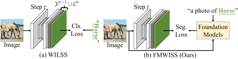
Figure 1: Illustration of the major difference of pipeline between previous WILSS work and FMWISS. Given a model pre-trained on old classes with pixel-level labels ($\mathcal{Y}^{t-1}$), previous work [8] learn new classes (e.g., horse) via image-level labels ($\mathcal{C}^{t}$), while FMWISS improves and effectively utilizes the supervision from complementary foundation models.

Semantic segmentation is a fundamental task in computer vision and has witnessed great progress using deep learning in the past few years. It aims at assigning each pixel a category label. Modern supervised semantic segmentation methods [12, 14] are usually based on published large-scale segmentation datasets with pixel annotations. Despite the promising results, one model pre-trained on one dataset is prone to easily forget learned knowledge when being retrained on another dataset with new classes. This phenomenon is known as catastrophic forgetting [37], which is caused by large changes of model parameters to model new samples with novel categories without accessing old samples.

A promising approach to solve such catastrophic forgetting problem is called incremental learning. Many methods have been proposed to solve image classification task [28, 10, 50, 33, 17, 44, 7, 46, 25, 49, 41]. Recently, a few methods have been presented to address incremental learning for semantic segmentation (ILSS) task, where only new classes of training samples of the current step are labeled with pixel annotations and old classes of the previous step are labeled as background. Modern ILSS methods can be classified into two categories: regularization-based and replay-based. Regularization-based methods [9, 18, 39] focus on distilling knowledge, e.g., output probability, intermedia features, from pre-trained model of previous step. Replay-based methods [36] propose to store the information of previous old classes or web-crawled images and replay for new training steps. However, a key barrier to further develop these methods is the requirement for pixel-level annotations for new classes. Very recently, WILSON [8] first proposes a new task, weakly incremental learning for semantic segmentation (WILSS), to incrementally update the model from image-level labels for new classes. Despite the comparable results, the image-level labels can not provide details to accurately locate each segment, which limits the performance and development of WILSS.

In this work, we explore to improve and more effectively utilize the supervision of new classes given image-level labels while preserving the knowledge of old ones. We propose a Foundation Model drives Weakly Incremental learning for Semantic Segmentation framework, dubbed FMWISS.

Firstly, as shown in Figure 1, we are the first attempt to leverage pre-trained foundation models to improve the supervision given image-level labels for WILSS in a training-free manner. To be specific, we propose pre-training based co-segmentation to distill the knowledge of vision-language pre-training models (e.g., CLIP [42]) and self-supervised pre-training models (e.g., iBOT [52]), which can be complementary to each other. However, it is not trivial to apply the pre-trained models. We first adapt CLIP for category-aware dense mask generation. Based on the initial mask for each new class, we then propose to extract compact category-agnostic attention maps with seeds guidance using self-supervised models. We finally refine the pseudo masks via mask fusion. We further propose to optimize the still noisy pseudo masks with a teacher-student architecture, where the plug-in teacher is optimized with the proposed dense contrastive loss. Thus we can more effectively utilize the pseudo dense supervision. Finally, we present memory-based copy-paste augmentation to remedy the forgetting problem of old classes and can further improve the performance.

The contributions of this paper are as follows:

• We present a novel and data-efficient WILSS framework, called FMWISS, which is the first attempt to utilize complementary foundation models to improve and more effectively use the supervision given only image-level labels.

• We propose pre-training based co-segmentation to generate dense masks by distilling both category-aware and category-agnostic knowledge from pre-trained foundation models, which provides dense supervision against original image labels.

• To effectively utilize pseudo labels, we use a teacher-student architecture with a proposed dense contrastive loss to dynamically optimize the noisy pseudo labels.

• We further introduce memory-based copy-paste augmentation to remedy the forgetting problem of old classes and can also improve performance.

• Extensive experiments on Pascal VOC and COCO datasets demonstrate the significant efficacy of our FMWISS framework.

2 Related Work

Incremental Learning for Semantic Segmentation. In addition to an exhaustive exploration of incremental learning for image classification [28, 10, 50, 33, 17, 44, 7, 46, 25, 49, 41], a relatively few methods [9, 18, 29, 36, 38, 39] have been proposed to tackle the incremental learning for semantic segmentation task, which can be classified into regularization-based and replay-based methods. Regularization-based methods [9, 18, 39] focus on preserving knowledge from previous training steps. For instance, MiB [9] proposes a modified version of traditional cross-entropy and knowledge distillation loss terms to regularize the probability of old classes and distill previous knowledge respectively, so as to remedy the background shift problem. PLOP [18] proposes a multi-scale pooling technique to preserve long and short-range spatial relationships at the feature level. SDR [39] proposes to optimize the class-conditional features by minimizing feature discrepancy of the same class. In addition, as a replay-based method, RECALL [36] uses web-crawled images with pseudo labels to remedy the forgetting problem. Pixel-by-pixel labeling for semantic segmentation is time-consuming and labor-intensive. Recently, some literature proposes to attain segmentations from cheaper and more available supervisions, e.g., sparse point [4], and image-level label [26, 31, 47], which has been attracting more and more attention these years. Most image-based weakly supervised semantic segmentation methods [3, 32, 48] leverage image-level labels to optimize the class activation map (CAM) and then extract pseudo dense annotations. However, the image-level label is rarely explored in incremental learning for semantic segmentation.

Very recently, WILSON [8] first proposes a novel weakly incremental learning for semantic segmentation (WILSS) task, which extends a pre-trained segmentation model using only image-level labels and achieves comparable results. In this work, inspired by WILSON [8], we present a FMWISS framework to improve and effectively utilize the image-level labels by distilling the knowledge of the complementary foundation models.

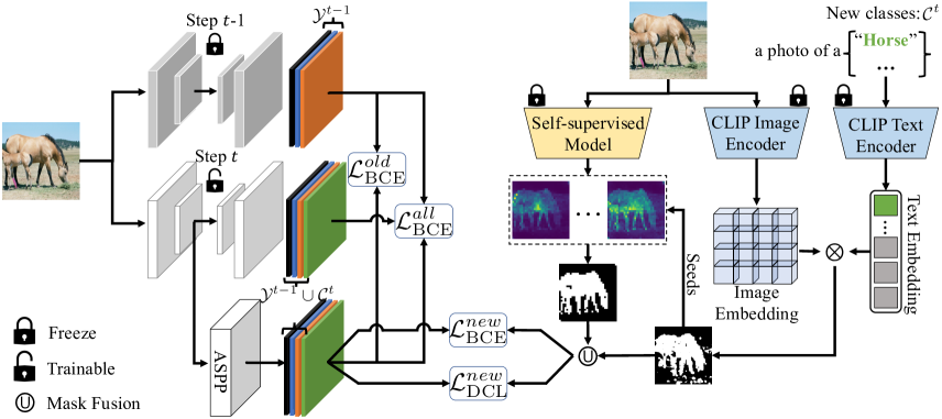
Figure 2: Illustration of the proposed FMWISS framework. The plug-in teacher module (ASPP [11]) is to learn the segments of both old and new classes during training, which is eliminated during inference. The model at step t is optimized using the outputs of the pre-trained model at step t-1 and the learned logits of the online teacher module.

Visual Foundation Models. We mainly focus on two kinds of foundation models in computer vision, including the vision-language pre-training (VLP) models and the self-supervised pre-training models. VLP [42, 27] plays an important role in multimodal research, e.g., VQA [2], text-to-image generation [43], zero-shot classification [53, 54]. A representative VLP work is CLIP [42], which jointly trains the image and text encoders on 400 million image-text pairs collected from the web and demonstrates promising results on zero-shot image classification tasks. Recently, MaskCLIP [51] adapts CLIP to zero-shot semantic segmentation in a training-free manner, which illustrates the potential of CLIP in category-aware dense prediction. Self-supervised visual pre-training can be classified into three categories: contrastive learning based [40, 15, 23], distillation based [20, 6], and masked image modeling based [22, 52]. Among these methods, iBOT [52] and DINO [6] are two representative approaches to automatically perform class-agnostic dense features modeling. These two kinds of foundation models can be complementary to each other.

3 Method

3.1 Problem Definition and Notation

Let $\mathcal{X}$ be the input image space and each image $x\in\mathcal{X}$ consists of a set of pixels $\mathcal{I}$ with $|\mathcal{I}|=H\times W$. Let $\mathcal{Y}$ be the label space. In the incremental learning for semantic segmentation setting [9], the training procedure is arranged into multiple steps, and each learning step $t$ will involve novel classes $\mathcal{C}^{t}$ with pixel annotations, constructing a new label set $\mathcal{Y}^{t}=\mathcal{Y}^{t-1}\cup\mathcal{C}^{t}$. However, different from the original incremental setting, in the novel weakly incremental learning for semantic segmentation (WILSS) setting, recently proposed by WILSON [8], the pixel annotations are only provided for the initial step, i.e., $t=0$. For the following steps, we can only access to training sets with image-level annotations for new classes, and can not access to the training samples of previous training steps anymore. The goal is to learn and update a model to perform segmentation on new classes without forgetting old classes.

3.2 Pre-training Based Co-segmentation

It is still challenging to use only image-level labels to supervise the dense prediction tasks, e.g., semantic segmentation, since image-level labels can not provide detailed information to accurately locate each segment. This limitation inspires us to investigate the following question: how to improve the supervision of new classes from image-level labels? To tackle this question, we propose a pre-training based co-segmentation method to utilize the knowledge of foundation models in a training-free manner. We distill the complementary knowledge of two kinds of foundation models, including the vision-language pre-training models, e.g., CLIP [42], and the self-supervised pre-training models, e.g., iBOT [52], DINO [6].

Initial Mask. We believe that the pre-trained vision-language model, e.g., CLIP, has encoded rich semantic information in its features as it learns to associate image with language caption from 400 million image-text pairs. To get dense prediction of a new class image, we apply the pre-trained CLIP model to extract category-aware pixel annotations given image-level labels. As shown in Figure 2, to be specific, given an image $x$ of step $t$ with image-level labels $\mathcal{C}^{t}$, we first extract dense image features $F$ from the CLIP image encoder $f_{I}$. Then, project $F$ via the final linear projection layer $f_{proj}$ of $f_{I}$.

$$\overline{F}=|f_{proj}(F)|_{2},~{}~{}\overline{F}\in\mathbb{R}^{h\times w\times d},$$ (1)

where $|\cdot|_{2}$ denotes L2 normalization along the channel dimension, $d$ is the feature dimension of the joint space. We then compute the text embeddings by taking as input the prompt with target classes $\mathcal{C}^{t}$ of step $t$:

$$\overline{T}=|f_{T}({\tt prompt}(\mathcal{C}^{t}))|_{2},~{}~{}\overline{T}\in\mathbb{R}^{\mathcal{C}^{t}\times d},$$ (2)

where $f_{T}$ is the CLIP text encoder, ${\tt prompt}(\cdot)$ denotes prompt engineering, which ensembles multiple prompt templates as in [42].

We then compute the pixel-text score maps using the language-compatible image feature embeddings $\overline{F}$ and the text embeddings $\overline{T}$ by:

$$\mathcal{M}_{init}=\overline{F}\cdot\overline{T}^{\top},~{}\mathcal{M}_{init}\in\mathbb{R}^{h\times w\times\mathcal{C}^{t}},$$ (3)

which indicates that each pixel will be assign a score for each class in $\mathcal{C}^{t}$, and $\mathcal{M}_{init}$ can be viewed as the initial segmentation results with category information.

Refine Mask via Seeds Guidance. The pseudo mask $\mathcal{M}_{init}$ generated by CLIP [42] can provide rich category-aware pixel annotations, but the mask is noisy since the training paradigm of CLIP based on image-text pairs doomed to be good at instance-level classification rather than segmentation. To improve the mask quality, we propose to distill the knowledge of another kind of foundation models, i.e., self-supervised pre-training models, which have shown promising performance in local feature modeling [6, 52]. These models can produce compact category-agnostic attention maps. However, how to extract segmentations for a target class given an image that may contain multiple objects? To address this issue, we propose to refine the initial mask via category-specific seeds guidance. Specifically, we randomly select $N=\{(i_{p},j_{p})\}^{N}_{p=1}$ seed points from initial mask $\mathcal{M}_{init}\in\mathbb{R}^{h\times w\times\mathcal{C}^{t}}$ for each target class $c\in\mathcal{C}^{t}$, and extract the corresponding attention maps from the pre-trained self-supervised model. Let $S$ denotes the image encoder of the self-supervised model, $S(x)\in\mathbb{R}^{h\times w\times n}$ denotes the output attention maps of the last self-attention block. We extract the category-aware attention map with the guidance of seeds as follows. For simplicity, we only show the calculation on one class $c\in\mathcal{C}^{t}$:

$$\mathcal{M}^{c}_{seeds}=\big{[}\frac{1}{N}\sum^{N}_{p=1}\frac{1}{n}\sum^{n}S(x)\big{]}_{\tt binary},$$ (4)

where $n$ denotes the number of attention heads. The $N$ seed points are randomly sampled from the foreground of binarized $\mathcal{M}_{init}$ for each new class and training step. $[\cdot]_{\tt binary}$ is a binarization operation that sets all the values greater than the threshold $\mathcal{T}$ to 1, otherwise 0. $\mathcal{T}$ is dynamically updated to keep the top $\mathcal{K}$% ($\mathcal{K}=70$ by default) locations from the averaged attention map. As shown in Figure 5, we visualize extracted attention maps of two classes (horse, dog), nine seeds ($N=9$) can already show good clustering performance.

Finally, we get the refined mask via simple mask fusion for better performance:

$$\mathcal{M}_{refine}=\mathcal{M}_{init}\cup\mathcal{M}_{seeds},~{}~{}\mathcal{M}_{refine}\in\mathbb{R}^{h\times w\times\mathcal{C}^{t}},$$ (5)

where $\cup$ represents mask fusion operation, which is the union operation in our experiments by default.

3.3 Pseudo Label Optimization

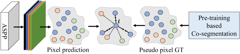
Figure 3: Illustration of the dense contrastive loss calculation process. The colorful points represent pixels with different categories.

Previous WILSS literature [8] use learned CAM to supervise the segmentation learning of new classes, and CAM is optimized with a binary cross-entropy (BCE) loss against one-hot image-level labels. Now, we have the generated pseudo pixel labels that can provide more information than image-level labels, a natural question is: how to effectively utilize such supervision?

We propose to use a teacher-student architecture to further optimize the still noisy pseudo mask. To be specific, by taking the segmentation model as student model, we introduce a plug-in teacher module (ASPP network in Figure 2) to dynamically learn better pseudo masks during training. To learn the teacher module, we first propose to use the pixel-wise binary cross-entropy loss $\mathcal{L}^{new}_{\text{BCE}}$ to supervise the predictions of the new classes at step $t$ as follows, and we leave the old classes optimization in the next section.

$$\begin{split}\mathcal{L}^{new}_{\text{BCE}}=-\frac{1}{|\mathcal{C}^{t}||\mathcal{I}|}\sum_{i\in\mathcal{I}}\sum_{c\in\mathcal{C}^{t}}\mathcal{M}^{c,i}_{refine}\log(p^{c,i})\\ +(1-\mathcal{M}^{c,i})\log(1-p^{c,i}),\end{split}$$ (6)

where $p^{c,i}$ denotes the predicted probability on new class $c$ of pixel $i$. However, the pixel-wise BCE loss mainly focus on the optimization of the target foreground class $c$ of current input image and treat all other classes as background, which ignores the correlation among pixels. To better utilize the multi-class predictions and corresponding pixel-wise pseudo labels among the entire dataset, inspired by the InfoNCE [40] loss in unsupervised representation learning, we propose to perform dense contrastive learning.

Specifically, as depicted in Figure 3, for a pixel $i$ of a new class image and its corresponding pseudo annotation, we collect all the pixels with the same class label as $i$ to compose positive samples $\mathbf{P}_{i}$, and collect the points of other classes to compose negative samples $\mathbf{N}_{i}$. Formally, our dense contrastive loss $\mathcal{L}^{new}_{\text{DCL}}$ can be calculated as follows. For simplicity, we only show the loss on pixel $i$:

$$\mathcal{L}^{new}_{\text{DCL}}$$ (7)

$$=\frac{1}{|\mathbf{P}_{i}|}\sum_{q_{+}\in\mathbf{P}_{i}}-\log\frac{\text{exp}(i\cdot q_{+}/\tau)}{\text{exp}(i\cdot q_{+}/\tau)+\sum\limits_{q_{-}\in\mathbf{N}_{i}}\text{exp}(i\cdot q_{-}/\tau)},$$

where $\tau$ is a temperature term (0.1 by default). For training efficiency, we randomly sample only ten points for each contained class of the current mini-batch.

The pixel-wise BCE loss in Eq. (6) and the dense contrastive loss in Eq. (7) can be complementary to each other, which help the teacher module to learn discriminative pixel features as well as regularize the pixel feature space by intra-class and inter-class pixel feature modeling.

3.4 Memory-based Copy-Paste Augmentation

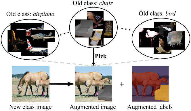
Figure 4: Illustration of the memory-based copy-paste augmentation. Notably, we will not use the ground-truth labels of new classes of augmented labels.

In addition to improving and effectively leveraging the supervision of new classes for WILSS, we propose a memory-based copy-paste augmentation strategy to stabilize the learning of old classes and can further improve the performance of the segmentation model. As shown in Figure 4, we first construct a memory bank for each old class, and each class archive will store $\mathcal{B}$ foreground instances and segmentation labels during the base model training. Then, in step $t$, we randomly pick one pair of foreground images and labels from a randomly selected old class archive, and randomly paste them to the new class image. Now, the training samples contain new class images at step $t$ as well as old class images and pixel labels at step $t$-1. We thus optimize the old class learning of the teacher module as:

$$\begin{split}\mathcal{L}^{old}_{\text{BCE}}=-\frac{1}{|\mathcal{Y}^{t-1}||\mathcal{I}|}\sum_{i\in\mathcal{I}}\sum_{c\in\mathcal{Y}^{t-1}}g(f^{t-1}_{\theta}(\hat{x}))^{c,i}\log(p^{c,i})\\ +(1-g(f^{t-1}_{\theta}(\hat{x}))^{c,i})\log(1-p^{c,i}),\end{split}$$ (8)

$$g(f^{t-1}_{\theta}(\hat{x}))^{c,i}=\begin{cases}1,&\hat{x}^{c,i}~{}\text{augmented},\\ g(f^{t-1}_{\theta}(\hat{x}))^{c,i},&\text{otherwise},\end{cases}$$ (9)

where $g(\cdot)$ is the logistic function, $f^{t-1}_{\theta}$ is the trained model at step $t$-1, $p^{c,i}$ is the predicted probability on old class $c$ of pixel $i$, $\hat{x}$ denotes the augmented image.

3.5 Overall Optimization

We optimize the segmentation model $f_{\theta}^{t}$ at step $t$ by distilling the knowledge of the trained model $f^{t-1}_{\theta}$ and the dynamically updated teacher module $T^{t}$. Since $T^{t}$ is optimized mainly through the binary cross-entropy loss, we use the BCE loss to distill the prediction of $T^{t}$ to model $f_{\theta}^{t}$. Considering that the learned pseudo mask is not perfect, we use the soft pixel labels as the final supervision for new classes $\mathcal{C}^{t}$, and use the weighted average value of the old model and teacher module outputs as the supervision for old classes:

$$q^{c,i}=\begin{cases}\alpha|T^{t}(x)|_{\text{hard}}+(1-\alpha)g(T^{t}(x)),&\text{if}~{}c\in\mathcal{C}^{t},\\ \beta g(f_{\theta}^{t-1}(x))+(1-\beta)g(T^{t}(x)),&\text{otherwise},\end{cases}$$ (10)

where $|\cdot|_{\text{hard}}$ denotes one-hot operation to set one to the class with the maximum score for each pixel and zero to others. $\alpha$ and $\beta$ are trade-off parameters and we set $\alpha=0.5,\beta=0.9$ by default. Then, the BCE loss for $f_{\theta}^{t}$ is:

$$\begin{split}\mathcal{L}^{all}_{\text{BCE}}=-\frac{1}{|\mathcal{Y}^{t}||\mathcal{I}|}\sum_{i\in\mathcal{I}}\sum_{c\in\mathcal{Y}^{t}}q^{c,i}\log(p^{c,i})\\ +(1-q^{c,i})\log(1-p^{c,i}),\end{split}$$ (11)

where $\mathcal{Y}^{t}$ is the set of all seen classes and $p=f_{\theta}^{t}(x)$ represents the output of segmentation model at step $t$.

The overall learning objective is as follows:

$$\mathcal{L}_{overall}=\mathcal{L}^{new}_{\text{BCE}}+\lambda\mathcal{L}^{new}_{\text{DCL}}+\mathcal{L}^{old}_{\text{BCE}}+\mathcal{L}^{all}_{\text{BCE}},$$ (12)

where $\lambda$ is the loss weight of $\mathcal{L}^{new}_{\text{DCL}}$.

4 Experiments

4.1 Datasets and Protocols

To ensure a fair comparison, we follow the experimental settings of the state-of-the-art (SoTA) WILSS method WILSON [8] for datasets and protocols. Different from [9, 36] rely on pixel-wise annotation on new classes, we only use image-level labels for novel classes as WILSON.

Datasets: we consider two standard evaluation benchmarks including Pascal VOC 2012 [19] and COCO [35]. COCO consists of 118,287 and 5,000 images for training and validation with 80 annotated object classes. Pascal VOC is composed of 1,464 training and 1,449 validation images with 20 labeled object classes. We follow the standard method [1, 30, 8] to augment the VOC dataset with images from [21], building up 10,582 and 1,449 images for training and validation, respectively. We also follow the practice of [8] to use the train split and the annotation of COCO-Stuff [5] that addresses the annotation overlapping problem of COCO [35].

Protocols: previous works [9] introduce two different incremental learning protocols: disjoint and overlap. In disjoint, images of each training step only contain pixels of previous seen and current classes. In overlap, each training step contains all the images, where pixels can belong to any class. Thus, the overlap protocol is more realistic and challenging compared to the disjoint. In our experiments, we follow the previous WILSS work [8] to apply these two protocols on the VOC dataset, including 15-5 VOC, where 15 base classes are learned in the first training step and 5 new classes are continuously learned in the second step; 10-10 VOC, where 10 base classes are learned in the first step and another 10 new classes are added in the second step. In addition, we also verify our method on the COCO-to-VOC protocol, which is a new incremental learning scenario proposed in [8]. To be specific, in the first step, we learn the 60 classes of COCO that do not appear in the VOC dataset. Then, we continuously learn the 20 classes of VOC. Following common practice [9, 36, 8], we report the standard mean Intersection over Union (mIoU) results on the validation sets.

4.2 Implementation Details

As in WILSON [8], we use a Deeplab V3 [13] with a ResNet-101 [24] backbone for VOC and a Wide-ResNet-38 for COCO, both pre-trained on ImageNet [16]. We train all the models for 40 epochs with a batch size of 24 and the SGD optimizer with a learning rate of 1$e^{-3}$, momentum of 0.9, weight decay of 1$e^{-4}$. Before training the segmentation model, we first warm up the teacher module for five epochs. We set $\lambda=0.1$, $\alpha=0.5$, and $\beta=0.9$. As for foundation models, in terms of the VLP model, we find that MaskCLIP [51] is an alternative solution to adapt CLIP for better dense prediction, and we use its mechanism based on the pre-trained CLIP with ViT-B architecture. In terms of the self-supervised model, we use pre-trained iBOT [52] with ViT-L architecture by default.

4.3 Baselines

Since weakly incremental learning for semantic segmentation (WILSS) is a novel setting proposed by WILSON [8], we also compare our framework with both supervised incremental learning and weakly supervised semantic segmentation methods as in [8]. For supervised incremental learning methods using dense pixel-wise annotations, we compare with eight representative state-of-the-art works, including LWF [34], LWF-MC [45], ILT [38], MiB [9], PLOP [18], CIL [29], SDR [39], and RECALL [36]. As for the weakly supervised semantic segmentation methods adopted to the incremental learning scenario, we compare with the reported results with the pseudo labels generated from class activation maps (CAM), SEAM [48], SS [3], and EPS [32] as in [8].

4.4 Results.

4.4.1 Performance on 15-5 VOC

In this setting, for a fair comparison, we also introduce 5 classes in the incremental step as in [8]: plant, sheep, sofa, train, tv monitor. As shown in Table 1, our FMWISS achieves the new state-of-the-art results in all the settings (disjoint and overlap) compared to all the pixel label based and image label based methods. To be more specific, compared to pixel label based methods, our WILSS method FMWISS even outperforms the best method by 3.5% and 3.2% in the two settings, respectively. Compared to image label based methods, FMWISS improves the overall performance by 3.4% and 6.1% in the two settings against previous SoTA WILSON [8]. Notably, FMWISS significantly improves the performance on new classes (16-20) by 7.0% and 12.8% in the disjoint and overlap settings, respectively.

Method	Sup	Disjoint			Overlap
		1-15	16-20	All	1-15	16-20	All
Joint∗	P	75.5	73.5	75.4	75.5	73.5	75.4
FT∗	P	8.4	33.5	14.4	12.5	36.9	18.3
LWF∗ [34]	P	39.7	33.3	38.2	67.0	41.8	61.0
LWF-MC∗ [45]	P	41.5	25.4	37.6	59.8	22.6	51.0
ILT∗ [38]	P	31.5	25.1	30.0	69.0	46.4	63.6
CIL∗ [29]	P	42.6	35.0	40.8	14.9	37.3	20.2
MIB∗ [9]	P	71.8	43.3	64.7	75.5	49.4	69.0
PLOP [18]	P	71.0	42.8	64.3	75.7	51.7	70.1
SDR∗ [39]	P	73.5	47.3	67.2	75.4	52.6	69.9
RECALL∗ [36]	P	69.2	52.9	66.3	67.7	54.3	65.6
CAM†	I	69.3	26.1	59.4	69.9	25.6	59.7
SEAM† [48]	I	71.0	33.1	62.7	68.3	31.8	60.4
SS† [3]	I	71.6	26.0	61.5	72.2	27.5	62.1
EPS† [32]	I	72.4	38.5	65.2	69.4	34.5	62.1
WILSON† [8]	I	73.6	43.8	67.3	74.2	41.7	67.2
FMWISS (Ours)	I	75.9 (+2.3)	50.8 (+7.0)	70.7 (+3.4)	78.4 (+4.2)	54.5 (+12.8)	73.3 (+6.1)

Table 1: Results on the 15-5 setting of Pascal VOC. ^∗ denotes the results are from [36], ^† denotes the results are from [8]. ‘P’ and ‘I’ indicate pixel-level and image-level labels, respectively. The best methods of using image-level labels and using pixel-level labels as supervision are bold and underlined, respectively.

4.4.2 Performance on 10-10 VOC

In this setting, for a fair comparison, we also introduce 10 classes in the incremental step as in [8]: dining table, dog, horse, motorbike, person, plant, sheep, sofa, train, tv monitor. As reported in Table 2, our FMWISS achieves the new state-of-the-art performance against the image label based methods and achieves on par or even better performance than the pixel label based methods. Specifically, compared to pixel label based methods, we achieve an overall performance of 64.6% on disjoint protocol, which is very close to ILT’s 64.7%. On overlap protocol, we achieve an overall performance of 69.1%, which is even 1.8% higher than SDR’s 67.4%. Compared to image label based methods, our FMWISS achieves the best results on all the protocols, and we achieve overall performance improvements of 3.8% and 4.1% in both settings compared to WILSON [8].

Method	Sup	Disjoint			Overlap
		1-10	11-20	All	1-10	11-20	All
Joint∗	P	76.6	74.0	75.4	76.6	74.0	75.4
FT∗	P	7.7	60.8	33.0	7.8	58.9	32.1
LWF∗ [34]	P	63.1	61.1	62.2	70.7	63.4	67.2
LWF-MC∗ [45]	P	52.4	42.5	47.7	53.9	43.0	48.7
ILT∗ [38]	P	67.7	61.3	64.7	70.3	61.9	66.3
CIL∗ [29]	P	37.4	60.6	48.8	38.4	60.0	48.7
MIB∗ [9]	P	66.9	57.5	62.4	70.4	63.7	67.2
PLOP [18]	P	63.7	60.2	63.4	69.6	62.2	67.1
SDR∗ [39]	P	67.5	57.9	62.9	70.5	63.9	67.4
RECALL∗ [36]	P	64.1	56.9	61.9	66.0	58.8	63.7
CAM†	I	65.4	41.3	54.5	70.8	44.2	58.5
SEAM† [48]	I	65.1	53.5	60.6	67.5	55.4	62.7
SS† [3]	I	60.7	25.7	45.0	69.6	32.8	52.5
EPS† [32]	I	64.2	54.1	60.6	69.0	57.0	64.3
WILSON† [8]	I	64.5	54.3	60.8	70.4	57.1	65.0
FMWISS (Ours)	I	68.5 (+4.0)	58.2 (+3.9)	64.6 (+3.8)	73.8 (+3.4)	62.3 (+5.2)	69.1 (+4.1)

Table 2: Results on the 10-10 setting of Pascal VOC. ^∗ denotes the results are from [36], ^† denotes the results are from [8].

4.4.3 Performance on COCO-to-VOC

This is a more challenging setting. First, the base model is trained on 60 classes of the COCO dataset, which are not overlapped with VOC. Then we train the additional 20 classes from VOC dataset with image-level labels in the second step. The results are reported in Table 3, FMWISS also achieves the new state-of-the-art performance against the WILSS methods.

Method	Sup	COCO			VOC
		1-60	61-80	All	61-80
FT†	P	1.9	41.7	12.7	75.0
LWF† [34]	P	36.7	49.0	40.3	73.6
ILT† [38]	P	37.0	43.9	39.3	68.7
MIB† [9]	P	34.9	47.8	38.7	73.2
PLOP† [18]	P	35.1	39.4	36.8	64.7
CAM†	I	30.7	20.3	28.1	39.1
SEAM† [48]	I	31.2	28.2	30.5	48.0
SS† [3]	I	35.1	36.9	35.5	52.4
EPS† [32]	I	34.9	38.4	35.8	55.3
WILSON† [8]	I	39.8	41.0	40.6	55.7
FMWISS (Ours)	I	39.9 (+0.1)	44.7 (+3.7)	41.6 (+1.0)	63.6 (+7.9)

Table 3: Results on the COCO-to-VOC setting. ^† denotes the results are from [8].

4.5 Ablation Studies

Unless otherwise specified, we perform the ablation experiments with iBOT [52] as the self-supervised model with ViT-B architecture based on the 10-10 VOC setting. We provide more ablation details, e.g., ablations of $\alpha,\beta,\mathcal{K}$, in our ${\tt supplementary}$ materials.

4.5.1 Effect of Number of Seeds

As depicted in Figure 5, we visualize the impact of number of seeds when calculating $\mathcal{M}_{seeds}$. Based on the category-aware $\mathcal{M}_{init}$ of two classes (horse, dog), more random seeds guidance leads to more compact attention maps and nine seeds are enough to get good clustering results for training efficiency. Moreover, the category-agnostic $\mathcal{M}_{seeds}$ can be complementary to the initial $\mathcal{M}_{init}$, which is indicated by red boxes.

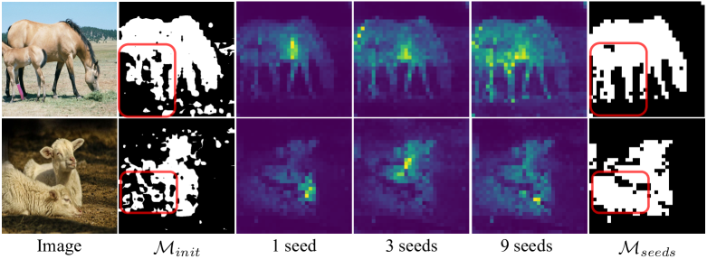
Figure 5: Effect of the number of randomly selected seeds.

4.5.2 Analysis of Mask Fusion

In this section, we verify the effect of mask fusion operation in Eq. (5). As shown in Table 4, we compare the results of two fusion operations and the result without fusion (“None”). Performing co-segmentation with “Union” can significantly improve performance, especially on new classes (53.25% $\rightarrow$ 55.45%, 56.39% $\rightarrow$ 60.54%). The results indicate that the proposed pre-training based co-segmentation does improve the supervision and performance for WILSS against original image-level labels.

Fusion	Disjoint			Overlap
Operation	1-10	11-20	All	1-10	11-20	All
None	67.83	53.25	61.96	73.25	56.39	66.45
Intersection	66.85	51.17	60.40	74.12	54.02	64.95
Union	67.23	55.45	62.74	73.12	60.54	67.94

Table 4: Performance comparison of the mask fusion operation. “None” denotes using only the $\mathcal{M}_{init}$ from CLIP.

4.5.3 Effect of Dense Contrastive Objective

We further analyze the effect of the proposed dense contrastive loss in Table 5. Compared to the result without using $\mathcal{L}^{new}_{\text{DCL}}$ ($\lambda=0.0$), introducing our proposed dense contrastive loss with a loss weight of 0.1 further improves the performance on new classes by 1.77% and 0.38% in the two settings, respectively. We thus set $\lambda=0.1$ in our experiments by default. The results show that the plug-in teacher module equipped with the proposed $\mathcal{L}^{new}_{\text{DCL}}$ can more effectively optimize and leverage the dense supervision for WILSS.

$\lambda$ of $\mathcal{L}^{new}_{\text{DCL}}$	Disjoint			Overlap
	1-10	11-20	All	1-10	11-20	All
0.0	67.23	55.45	62.74	73.12	60.54	67.95
0.1	67.94	57.22	63.91	73.44	60.92	68.28
1.0	67.15	57.94	63.87	72.08	61.05	68.17

Table 5: Ablation experiments on the dense contrastive objective $\mathcal{L}^{new}_{\text{DCL}}$. $\lambda=0.0$ represents eliminating the dense contrastive loss.

4.5.4 Effect of Memory-based Copy-paste Augmentation

As reported in Table 6, we analyze the effect of the proposed memory-based copy-paste augmentation. Without further tuning, we fix the augmentation probability as 0.5. Compared with the results without augmentation, applying the copy-paste augmentation with $\mathcal{B}=50$ can already improve the performance of old classes (67.94% $\rightarrow$ 68.64% in disjoint, 73.44% $\rightarrow$ 73.71% in overlap) for saving memory consumption.

Rand.	Memory-bank	Disjoint			Overlap
	$\mathcal{B}$	1-10	11-20	All	1-10	11-20	All
0.5	0	67.94	57.22	63.91	73.44	60.92	68.28
	10	68.85	57.14	64.29	73.11	61.50	68.40
	50	68.64	57.90	64.56	73.71	62.06	68.95
	100	68.41	58.09	64.55	73.26	61.78	68.60
	500	68.73	58.29	64.80	73.50	62.28	68.97

Table 6: Ablation experiments on the memory-based copy-paste augmentation. $\mathcal{B}=0$ denotes removing augmentation.

4.5.5 Effect of Different Self-supervised Models

We experiment with two representative self-supervised models [52, 6] based on different ViT architectures. As shown in Table 7, both bring promising results and we use iBOT with ViT-L for better and stable performance.

Self-supervised	Arch.	Disjoint			Overlap
Model		1-10	11-20	All	1-10	11-20	All
iBOT [52]	ViT-B	68.64	57.90	64.56	73.71	62.06	68.95
	ViT-L	68.51	58.20	64.64	73.79	62.26	69.09
DINO [6]	ViT-B	68.01	59.14	64.86	73.11	60.98	68.14
	ViT-S	66.86	58.85	64.17	70.97	59.57	66.43

Table 7: Performance comparison by using different self-supervised pre-training models.

4.5.6 Factor-by-factor Experiments

We conduct a factor-by-factor experiment on the proposed pre-training based co-segmentation, dense contrastive loss, and memory-based copy-paste augmentation. As shown in Tabel 8, each design has a positive effect, and all designs are combined to obtain the best performance.

Pre-training	$\mathcal{L}^{new}_{\text{DCL}}$	Copy-paste	Disjoint			Overlap
based Co-seg.		Aug.	1-10	11-20	All	1-10	11-20	All
			67.83	53.25	61.96	73.25	56.39	66.45
✓			67.23	55.45	62.74	73.12	60.54	67.94
✓	✓		67.94	57.22	63.91	73.44	60.92	68.28
✓	✓	✓	68.64	57.90	64.56	73.71	62.06	68.95
✓	✓	✓	68.51	58.20	64.64	73.79	62.26	69.09

Table 8: Effect of each design proposed in this work. The last row indicates the result of using ViT-L architecture.

Method	Sup	Disjoint			Overlap
		1-10	11-20	All	1-10	11-20	All
WILSON [8]	I	64.5	54.3	60.8	70.4	57.1	65.0
WILSON [8]	P	69.5	56.4	64.2	73.6	57.6	66.7
FMWISS (Ours)	I	68.5	58.2	64.6	73.8	62.3	69.1

Table 9: Comparison with previous WILSS SoTA [8] trained with direct dense annotations.

Method	Train	Disjoint			Overlap
	Data	1-10	11-20	All	1-10	11-20	All
WILSON [8]	100%	64.5	54.3	60.8	70.4	57.1	65.0
FMWISS (Ours)	100%	68.5	58.2	64.6	73.8	62.3	69.1
	50%	66.7	56.0	62.7	72.1	60.5	67.4
	30%	68.5	51.5	61.5	75.7	55.7	66.8

Table 10: Performance comparison with fewer training data.

4.5.7 Data Efficiency Experiment

We first compare with WILSON [8] trained with direct dense pixel-level labels (P) for all classes in Table 9. It is worth noting that FMWISS based on only image-level labels (I) still outperforms it, especially in the challenging overlap setting. We further evaluate FMWISS with fewer training data in Table 10. It is notable that FMWISS trained with only 30% data still outperforms WILSON trained with 100% data. Combining Table 9, Table 10, and the fast convergence result (Sec. 4) in supplementary materials, we can conclude that FMWISS is a significantly data-efficient WILSS framework.

4.5.8 Visualization

We report qualitative results indicating the superiority of our FMWISS framework on both old (e.g., bottle) and new (e.g., person, horse, dog, sofa) classes in Figure 6.

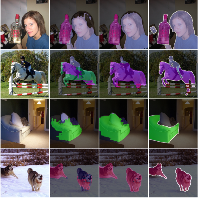
Figure 6: Qualitative comparison between previous WILSS SoTA [8] and our FMWISS on the 10-10 VOC setting. From left to right: image, WILSON [8], FMWISS and the ground-truth.

5 Limitations

Like WILSON [8], the FMWISS framework is not designed for single-class incremental learning steps, the proposed dense contrastive objective needs some other classes as negative samples.

6 Conclusion

In this paper, we present a novel and data-efficient FMWISS framework for weakly incremental learning for semantic segmentation. FMWISS is the first attempt to exploit knowledge of pre-trained foundation models for WILSS. We propose pre-training based co-segmentation to generate dense supervision based on image-level labels. We further use a teacher-student architecture with a proposed dense contrastive loss to more effectively utilize the pseudo labels. Besides, we introduce memory-based copy-paste augmentation to improve the forgetting problem of old classes. Extensive experiments demonstrate the superior results of FMWISS.

Appendix A Appendix

A.1 Effect of $\alpha$ and $\beta$

We analyze the sensitivity of $\alpha$ and $\beta$ and report the results in Table 11. First, we fix $\beta=1.0$ and find that equally ($\alpha=0.5$) integrating the hard and soft dense labels for new classes from the teacher can better improve the performance from 62.15% to 64.21%. Then, we fix $\alpha=0.5$ and find that paying more attention ($\beta=0.9$) to the outputs of old model $f^{t-1}_{\theta}$ than the teacher when supervise the old classes can achieve better overall performance. We set $\alpha=0.5,\beta=0.9$ in all our experiments by default.

Method	$\alpha$	$\beta$	1-10	11-20	All
FMWISS	0.0	1.0	67.19	54.30	62.15
	0.5		68.11	57.67	64.21
	1.0		67.20	57.64	64.13
	0.5	0.5	59.17	56.87	59.55
		0.7	64.73	57.23	62.37
		0.9	68.64	57.90	64.56
		1.0	68.11	57.67	64.21

Table 11: Ablation experiments on the parameters $\alpha$ and $\beta$ based on the disjoint protocol.

A.2 Number of Points in Dense Contrastive Loss

We analyze our FMWISS with different number of randomly sampled points when calculating the proposed $\mathcal{L}^{new}_{\text{DCL}}$. The results are reported in Table 12. We can see that FMWISS is robust to the number of sample points, and randomly sampling more points (e.g., 50) for each class may introduce more noise and thus degrade the performance. We randomly sample ten points when calculating $\mathcal{L}^{new}_{\text{DCL}}$ in our experiments by default.

Points in	Disjoint			Overlap
$\mathcal{L}^{new}_{\text{DCL}}$	1-10	11-20	All	1-10	11-20	All
5	68.37	58.18	64.56	73.64	62.38	69.04
10	68.51	58.20	64.64	73.79	62.26	69.09
50	68.67	57.72	64.49	73.35	61.67	68.58

Table 12: Ablation experiments on the number of points sampled for each contained class of the proposed dense contrastive loss.

A.3 Analysis of Mask Fusion

We analyze the impact of the $\mathcal{K}$ value when binarize $\mathcal{M}_{seeds}$, as shown in Table 13, preserving too little ($\mathcal{K}=90\%$) information from the self-supervised model can not utilize the complementary knowledge effectively, while keeping too much ($\mathcal{K}=60\%$) will introduce more noise. We thus set $\mathcal{K}=70\%$ for all other experiments.

$\mathcal{K}$ (%)	Disjoint			Overlap
	1-10	11-20	All	1-10	11-20	All
90	67.74	54.38	62.46	74.14	59.00	67.67
80	67.52	55.08	62.70	73.73	59.94	67.95
70	67.23	55.45	62.74	73.12	60.54	67.95
60	66.99	55.48	62.63	72.51	60.49	67.63

Table 13: Ablation experiments on the mask union operation by varying the percentage value $\mathcal{K}$.

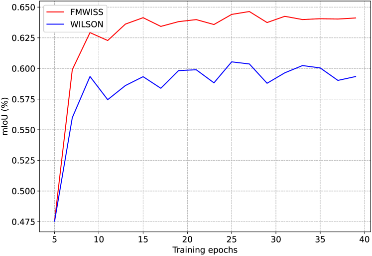
Figure 7: Convergence comparison between previous WILSS SoTA [8] and our FMWISS based on 10-10 VOC setting.

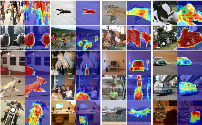
Figure 8: Qualitative visualization of the learned features maps of the teacher module on 10-10 VOC setting.

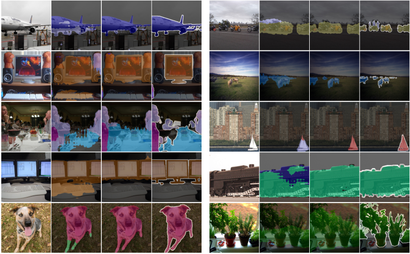
Figure 9: More qualitative comparison between previous WILSS SoTA [8] and our FMWISS on the 10-10 VOC setting. From left to right: image, WILSON [8], FMWISS (ours) and the ground-truth.

A.4 Analysis of Convergence

As shown in Figure 7, we report the convergence curve w.r.t. training process on the 10-10 VOC setting. We can conclude that our FMWISS can converge faster and can consistently improve the performance compared to the previous SoTA [8].

A.5 Visualization

To analyze the effect of the plug-in teacher module, we visualize the learned feature maps for all the old classes (aeroplane, bicycle, bird, boat, bottle, bus, car, cat, chair, cow) and all the new classes (dining table, dog, horse, motorbike, person, potted plant, sheep, sofa, train, tv monitor) based on the 10-10 VOC setting. As shown in Figure 8, it can be seen that the teacher module of FMWISS framework can learn clear and high attention scores for different correct classes.

As depicted in Figure 9, we show more qualitative results indicating the superiority of our FMWISS framework on both old (e.g., aeroplane, bottle, boat) and new (e.g., dog, motorbike, person, dining table, tv monitor, sheep, train, potted plant) classes.

References

- [1] Jiwoon Ahn and Suha Kwak. Learning pixel-level semantic affinity with image-level supervision for weakly supervised semantic segmentation. In CVPR, pages 4981–4990, 2018.
- [2] Stanislaw Antol, Aishwarya Agrawal, Jiasen Lu, Margaret Mitchell, Dhruv Batra, C Lawrence Zitnick, and Devi Parikh. Vqa: Visual question answering. In ICCV, pages 2425–2433, 2015.
- [3] Nikita Araslanov and Stefan Roth. Single-stage semantic segmentation from image labels. In CVPR, pages 4253–4262, 2020.
- [4] Amy Bearman, Olga Russakovsky, Vittorio Ferrari, and Li Fei-Fei. What’s the point: Semantic segmentation with point supervision. In ECCV, pages 549–565. Springer, 2016.
- [5] Holger Caesar, Jasper Uijlings, and Vittorio Ferrari. Coco-stuff: Thing and stuff classes in context. In CVPR, pages 1209–1218, 2018.
- [6] Mathilde Caron, Hugo Touvron, Ishan Misra, Hervé Jégou, Julien Mairal, Piotr Bojanowski, and Armand Joulin. Emerging properties in self-supervised vision transformers. In ICCV, pages 9650–9660, 2021.
- [7] Francisco M Castro, Manuel J Marín-Jiménez, Nicolás Guil, Cordelia Schmid, and Karteek Alahari. End-to-end incremental learning. In ECCV, pages 233–248, 2018.
- [8] Fabio Cermelli, Dario Fontanel, Antonio Tavera, Marco Ciccone, and Barbara Caputo. Incremental learning in semantic segmentation from image labels. In CVPR, pages 4371–4381, 2022.
- [9] Fabio Cermelli, Massimiliano Mancini, Samuel Rota Bulo, Elisa Ricci, and Barbara Caputo. Modeling the background for incremental learning in semantic segmentation. In CVPR, pages 9233–9242, 2020.
- [10] Arslan Chaudhry, Puneet K Dokania, Thalaiyasingam Ajanthan, and Philip HS Torr. Riemannian walk for incremental learning: Understanding forgetting and intransigence. In ECCV, pages 532–547, 2018.
- [11] Liang-Chieh Chen, George Papandreou, Iasonas Kokkinos, Kevin Murphy, and Alan L Yuille. Semantic image segmentation with deep convolutional nets and fully connected crfs. arXiv preprint arXiv:1412.7062, 2014.
- [12] Liang-Chieh Chen, George Papandreou, Iasonas Kokkinos, Kevin Murphy, and Alan L Yuille. Deeplab: Semantic image segmentation with deep convolutional nets, atrous convolution, and fully connected crfs. IEEE TPAMI, 40(4):834–848, 2017.
- [13] Liang-Chieh Chen, George Papandreou, Florian Schroff, and Hartwig Adam. Rethinking atrous convolution for semantic image segmentation. arXiv preprint arXiv:1706.05587, 2017.
- [14] Liang-Chieh Chen, Yukun Zhu, George Papandreou, Florian Schroff, and Hartwig Adam. Encoder-decoder with atrous separable convolution for semantic image segmentation. In ECCV, pages 801–818, 2018.
- [15] Ting Chen, Simon Kornblith, Mohammad Norouzi, and Geoffrey Hinton. A simple framework for contrastive learning of visual representations. In ICML, pages 1597–1607. PMLR, 2020.
- [16] Jia Deng, Wei Dong, Richard Socher, Li-Jia Li, Kai Li, and Li Fei-Fei. Imagenet: A large-scale hierarchical image database. In CVPR, pages 248–255. Ieee, 2009.
- [17] Prithviraj Dhar, Rajat Vikram Singh, Kuan-Chuan Peng, Ziyan Wu, and Rama Chellappa. Learning without memorizing. In CVPR, pages 5138–5146, 2019.
- [18] Arthur Douillard, Yifu Chen, Arnaud Dapogny, and Matthieu Cord. Plop: Learning without forgetting for continual semantic segmentation. In CVPR, pages 4040–4050, 2021.
- [19] Mark Everingham, Luc Van Gool, Christopher KI Williams, John Winn, and Andrew Zisserman. The pascal visual object classes (voc) challenge. IJCV, 88(2):303–338, 2010.
- [20] Jean-Bastien Grill, Florian Strub, Florent Altché, Corentin Tallec, Pierre Richemond, Elena Buchatskaya, Carl Doersch, Bernardo Avila Pires, Zhaohan Guo, Mohammad Gheshlaghi Azar, et al. Bootstrap your own latent-a new approach to self-supervised learning. NeurIPS, 33:21271–21284, 2020.
- [21] Bharath Hariharan, Pablo Arbeláez, Lubomir Bourdev, Subhransu Maji, and Jitendra Malik. Semantic contours from inverse detectors. In ICCV, pages 991–998. IEEE, 2011.
- [22] Kaiming He, Xinlei Chen, Saining Xie, Yanghao Li, Piotr Dollár, and Ross Girshick. Masked autoencoders are scalable vision learners. In CVPR, pages 16000–16009, 2022.
- [23] Kaiming He, Haoqi Fan, Yuxin Wu, Saining Xie, and Ross Girshick. Momentum contrast for unsupervised visual representation learning. In CVPR, pages 9729–9738, 2020.
- [24] Kaiming He, Xiangyu Zhang, Shaoqing Ren, and Jian Sun. Deep residual learning for image recognition. In CVPR, pages 770–778, 2016.
- [25] Saihui Hou, Xinyu Pan, Chen Change Loy, Zilei Wang, and Dahua Lin. Learning a unified classifier incrementally via rebalancing. In CVPR, pages 831–839, 2019.
- [26] Zilong Huang, Xinggang Wang, Jiasi Wang, Wenyu Liu, and Jingdong Wang. Weakly-supervised semantic segmentation network with deep seeded region growing. In CVPR, pages 7014–7023, 2018.
- [27] Chao Jia, Yinfei Yang, Ye Xia, Yi-Ting Chen, Zarana Parekh, Hieu Pham, Quoc Le, Yun-Hsuan Sung, Zhen Li, and Tom Duerig. Scaling up visual and vision-language representation learning with noisy text supervision. In ICML, pages 4904–4916. PMLR, 2021.
- [28] James Kirkpatrick, Razvan Pascanu, Neil Rabinowitz, Joel Veness, Guillaume Desjardins, Andrei A Rusu, Kieran Milan, John Quan, Tiago Ramalho, Agnieszka Grabska-Barwinska, et al. Overcoming catastrophic forgetting in neural networks. Proceedings of the national academy of sciences, 114(13):3521–3526, 2017.
- [29] Marvin Klingner, Andreas Bär, Philipp Donn, and Tim Fingscheidt. Class-incremental learning for semantic segmentation re-using neither old data nor old labels. In ITSC, pages 1–8. IEEE, 2020.
- [30] Alexander Kolesnikov and Christoph H Lampert. Seed, expand and constrain: Three principles for weakly-supervised image segmentation. In ECCV, pages 695–711. Springer, 2016.
- [31] Jungbeom Lee, Eunji Kim, Sungmin Lee, Jangho Lee, and Sungroh Yoon. Ficklenet: Weakly and semi-supervised semantic image segmentation using stochastic inference. In CVPR, pages 5267–5276, 2019.
- [32] Seungho Lee, Minhyun Lee, Jongwuk Lee, and Hyunjung Shim. Railroad is not a train: Saliency as pseudo-pixel supervision for weakly supervised semantic segmentation. In CVPR, pages 5495–5505, 2021.
- [33] Zhizhong Li and Derek Hoiem. Learning without forgetting. IEEE TPAMI, 40(12):2935–2947, 2017.
- [34] Zhizhong Li and Derek Hoiem. Learning without forgetting. IEEE TPAMI, 40(12):2935–2947, 2017.
- [35] Tsung-Yi Lin, Michael Maire, Serge Belongie, James Hays, Pietro Perona, Deva Ramanan, Piotr Dollár, and C Lawrence Zitnick. Microsoft coco: Common objects in context. In ECCV, pages 740–755. Springer, 2014.
- [36] Andrea Maracani, Umberto Michieli, Marco Toldo, and Pietro Zanuttigh. Recall: Replay-based continual learning in semantic segmentation. In ICCV, pages 7026–7035, 2021.
- [37] Michael McCloskey and Neal J Cohen. Catastrophic interference in connectionist networks: The sequential learning problem. In Psychology of learning and motivation, volume 24, pages 109–165. Elsevier, 1989.
- [38] Umberto Michieli and Pietro Zanuttigh. Incremental learning techniques for semantic segmentation. In ICCV Workshops, pages 0–0, 2019.
- [39] Umberto Michieli and Pietro Zanuttigh. Continual semantic segmentation via repulsion-attraction of sparse and disentangled latent representations. In CVPR, pages 1114–1124, 2021.
- [40] Aaron van den Oord, Yazhe Li, and Oriol Vinyals. Representation learning with contrastive predictive coding. arXiv preprint arXiv:1807.03748, 2018.
- [41] Oleksiy Ostapenko, Mihai Puscas, Tassilo Klein, Patrick Jahnichen, and Moin Nabi. Learning to remember: A synaptic plasticity driven framework for continual learning. In CVPR, pages 11321–11329, 2019.
- [42] Alec Radford, Jong Wook Kim, Chris Hallacy, Aditya Ramesh, Gabriel Goh, Sandhini Agarwal, Girish Sastry, Amanda Askell, Pamela Mishkin, Jack Clark, et al. Learning transferable visual models from natural language supervision. In ICML, pages 8748–8763. PMLR, 2021.
- [43] Aditya Ramesh, Prafulla Dhariwal, Alex Nichol, Casey Chu, and Mark Chen. Hierarchical text-conditional image generation with clip latents. arXiv preprint arXiv:2204.06125, 2022.
- [44] Sylvestre-Alvise Rebuffi, Alexander Kolesnikov, Georg Sperl, and Christoph H Lampert. icarl: Incremental classifier and representation learning. In CVPR, pages 2001–2010, 2017.
- [45] Sylvestre-Alvise Rebuffi, Alexander Kolesnikov, Georg Sperl, and Christoph H Lampert. icarl: Incremental classifier and representation learning. In CVPR, pages 2001–2010, 2017.
- [46] Hanul Shin, Jung Kwon Lee, Jaehong Kim, and Jiwon Kim. Continual learning with deep generative replay. NeurIPS, 30, 2017.
- [47] Guolei Sun, Wenguan Wang, Jifeng Dai, and Luc Van Gool. Mining cross-image semantics for weakly supervised semantic segmentation. In ECCV, pages 347–365. Springer, 2020.
- [48] Yude Wang, Jie Zhang, Meina Kan, Shiguang Shan, and Xilin Chen. Self-supervised equivariant attention mechanism for weakly supervised semantic segmentation. In CVPR, pages 12275–12284, 2020.
- [49] Chenshen Wu, Luis Herranz, Xialei Liu, Joost van de Weijer, Bogdan Raducanu, et al. Memory replay gans: Learning to generate new categories without forgetting. NeurIPS, 31, 2018.
- [50] Friedemann Zenke, Ben Poole, and Surya Ganguli. Continual learning through synaptic intelligence. In ICML, pages 3987–3995. PMLR, 2017.
- [51] Chong Zhou, Chen Change Loy, and Bo Dai. Denseclip: Extract free dense labels from clip. arXiv preprint arXiv:2112.01071, 2021.
- [52] Jinghao Zhou, Chen Wei, Huiyu Wang, Wei Shen, Cihang Xie, Alan Yuille, and Tao Kong. ibot: Image bert pre-training with online tokenizer. arXiv preprint arXiv:2111.07832, 2021.
- [53] Kaiyang Zhou, Jingkang Yang, Chen Change Loy, and Ziwei Liu. Learning to prompt for vision-language models. arXiv preprint arXiv:2109.01134, 2021.
- [54] Kaiyang Zhou, Jingkang Yang, Chen Change Loy, and Ziwei Liu. Conditional prompt learning for vision-language models. In CVPR, pages 16816–16825, 2022.