Sequential edge detection using joint hierarchical Bayesian learning

Abstract

This paper introduces a new sparse Bayesian learning (SBL) algorithm that jointly recovers a temporal sequence of edge maps from noisy and under-sampled Fourier data. The new method is cast in a Bayesian framework and uses a prior that simultaneously incorporates intra-image information to promote sparsity in each individual edge map with inter-image information to promote similarities in any unchanged regions. By treating both the edges as well as the similarity between adjacent images as random variables, there is no need to separately form regions of change. Thus we avoid both additional computational cost as well as any information loss resulting from pre-processing the image. Our numerical examples demonstrate that our new method compares favorably with more standard SBL approaches.

MSC Classification]15A29, 62F15, 65F22, 65K10, 68U10

1 Introduction

In applications such as environment monitoring rogers1996predicting ; azzali2000mapping and surveillance othman2012wireless ; wimalajeewa2017application , temporal sequences of images are compared to determine changes within the physical region of interest. When data are acquired indirectly, each image in the temporal sequence is typically first recovered individually, before any comparisons are made. However, if the scene contains rigid bodies, it is often enough to infer important surveillance and monitoring information from the corresponding time sequenced edge maps, gelb2017detecting ; GS2017 ; SVGR ; gelb2019reducing . This is useful because recovering an edge map may be more accurate as well as less costly than recovering a full scale image.

Sequential edge maps can be used more generally in image recovery processes. For example, the weights in weighted $\ell_{1}$ regularization methods are designed to be inversely proportional to the strength of the signal in the sparse domain (see e.g. candes2008enhancing ). Accurate edge maps can help to determine these weights off-line and in advance, as was demonstrated in adcock2019jointsparsity ; gelb2019reducing ; scarnati2019accelerated . Segmentation, classification and object-based change detection (see e.g. xiao2022sequential ) are also examples of procedures where edge information can improve the quality of the results.

The primary motivation in this investigation comes from spotlight synthetic aperture radar (SAR), where the phase history data may be considered as Fourier data, jakowatz2012spotlight . We therefore seek to recover a sequence of edge maps from multiple observations of noisy and under-sampled Fourier measurements at different time instances, while noting that our underlying methodology can be applied to other types of measurements with some modifications.

Several algorithms have been designed to recover the edges in a real-valued signal from (multiple) under-sampled and noisy Fourier measurements at a single instance in time, even in situations where missing bands of Fourier data would make it impossible to recover the underlying image, GS2017 ; SVGR ; viswanathan2012iterative . Many techniques have also been developed to recover the magnitude of a SAR image using a sequence of sub-aperture data acquisitions, again at a single instance in time, Cetin2005 ; ccetin2014sparsity ; moses2004wide ; stojanovic2008joint . In this case the images are first separately recovered, each corresponding to a single data acquisition. The final estimate at each pixel is then calculated as the weighted average of the recovered images. However, processing the individual measurements to recover a set of images before combining the joint information can lead to additional information loss, especially in the case of noisy and incomplete data collections, archibald2016image ; scarnati2019accelerated ; wasserman2015image ; xiao2022sequential . By contrast, exploiting redundant information without having to first recover separate images leads to more accurate image recovery, scarnati2019accelerated ; xiao2022sequential . Recovery algorithms that incorporate information from multi-measurement vectors are often referred to as MMV recovery algorithms, adcock2019jointsparsity ; chen2006theoretical ; cotter2005sparse .

In developing methods to recover temporal sequences of images from noisy and under-sampled Fourier measurements, changes such as translation and rotation that are expected to occur between the sequential data collections must also be accounted for. Thus none of the techniques mentioned in the preceding paragraph is suitable. By contrast, the sequential image recovery developed in xiao2022sequential employs a compressive sensing (CS) framework with regularization terms designed to both account for sparsity in the appropriate transform domain as well as to promote similarities in regions for which no change has been detected. Following the ideas in scarnati2019accelerated , the edge maps are generated without first recovering the images so that additional information is not lost due to processing. In this way inter-image temporal correlations between adjacent measurements can be better exploited. Although demonstrated to yield improved accuracy when compared to algorithms which separately recover each image in the sequence, that is, without using inter-image information, the method in xiao2022sequential is multi-step and relies on several hand-tuned parameters. Specifically, after the edge maps for each individual image are generated from the observed data, rigid objects must be constructed to determine the changed and unchanged regions between each adjacent image (so-called change masks), which would then in turn form the regularization term. This step typically requires some type of clustering algorithm, leading to both a loss of information due to the extra processing and a lack of robustness due to the additional hand-tuning of parameters. Finally, there is an assumption that a moving object is not contained within another (background) object. For example, one would have to remove the skull in a magnetic resonance image (MRI) brain scan in order to determine changes within.

Such concerns were initially addressed in xiao2022sequential1 . There, the method in xiao2022sequential was recast in a Bayesian framework, with an intra-image prior used to promote sparsity in the edges of each image, and a second inter-image prior used to promote the similarity of the unchanged-regions. By treating the similarity between adjacent images as a random variable, forming the rigid boundaries as an intermediate step was no longer required.

In this investigation we consider sequential edge map recovery (as opposed to sequential image recovery) which allows us to further simplify the approach introduced in xiao2022sequential1 by integrating both intra- and inter-image information into one prior. That is, we introduce a prior that simultaneously promotes intra-image sparsity and inter-image similarity. To this end, we note that the classic sparse Bayesian learning (SBL) tipping2001sparse ; wipf2011latent ; zhang2011sparse ; chen2016simultaneous ; zhang2021empirical requires a shared support of all the collected measurements to approximate edges. Such an assumption will clearly be violated when change occurs between sequential data collections. To compensate, our proposed method introduces a new set of hyper-parameters so that information outside the shared support is not considered in the joint estimation of the edge values. Our numerical examples demonstrate that by constructing the SBL algorithm in this way we are able to account for changes in each sequenced edge map. Such information can then be used in downstream processing as warranted by the particular application.

This rest of this paper is organized as follows. Section 2 provides the necessary background for our new method, which is introduced in Section 3. Numerical examples for both one- and two-dimensional signals are considered in Section 4. We also demonstrate how our method for recovering sequential edge maps can then be used for recovering sequential images. Concluding remarks are given in 5.

2 Preliminaries

Let $f_{j}\colon[-\pi,\pi]\to\mathbb{R}$ be a sequence of one-dimensional piecewise smooth functions at different times $j=1,\dots,J$. The corresponding Fourier samples are given as

$$\hat{f}_{j,l}=\frac{1}{2\pi}\int_{-\pi}^{\pi}f_{j}(s)e^{-ils}ds,\quad-\frac{n}{2}\leq l\leq\frac{n}{2}-1,\quad j=1,\dots,J.$$ (1)

We note that our approach is directly extendable to two-dimensional images, which will be demonstrated via the numerical experiments in Section 4.

Suppose the corresponding forward model for the observations of $f_{j}$ is given by

$$\bm{g}_{j}=F_{j}\bm{f}_{j},\quad j=1,\dots,J,$$ (2)

where $\bm{f}_{j}$ is the discrete approximation of $f_{j}$ at $n$ uniform grid points on $[-\pi,\pi]$ and $F_{j}\in\mathbb{C}^{n\times n}$ is the discrete Fourier transform forward operator. In our numerical experiments, each $F_{j}$ is missing an arbitrarily chosen band-width of frequencies, indicating that the data sequence is compromised in some way, as well as being under-sampled. Details regarding the missing band-width will be made explicit in Section 4. We further assume that each of the $J$ observations are corrupted with additive independent and identically distributed (iid) zero-mean Gaussian noise with unknown variance $\sigma^{2}$ given by

$$\bm{\epsilon}_{j}\sim\mathcal{N}\left(0,\beta^{-1}I_{n}\right),\quad j=1,\dots,J,$$ (3)

where $\beta^{-1}=\sigma^{2}$. The forward model (2) therefore becomes

$$\tilde{\bm{g}}_{j}=F_{j}\bm{f}_{j}+\bm{\epsilon}_{j},\quad j=1,\dots,J.$$ (4)

We seek to recover the sequential edge maps corresponding to the observations in (4) using a Bayesian framework. As already noted, the edge maps may be useful on their own or in downstream processing. Examples in Sections 4.2 demonstrate how the edge maps can be used effectively for sequential image recovery.

2.1 Edge Detection from Fourier data

Detecting the edges of a piecewise smooth signal or image from a finite number of Fourier samples, (1), is a well-studied problem. Due to its simple linear construction, here we employ the concentration factor (CF) method, initially developed in gelb1999detection . Below we briefly describe the CF method in the context of edge map recovery. For ease of notation we drop the $j$ and write $f=f_{j}$ since what follows applies to any $j=1,\dots,J$.

Consider the piecewise analytic function $f$ which has $K$ simple discontinuities located at $\{\xi_{k}\}_{k=1}^{\mathcal{K}}$ in $(-\pi,\pi]$. The corresponding jump function is defined as

$$[f](s)=f(s^{+})-f(s^{-}),$$ (5)

where $f(s^{+})$ and $f(s^{-})$ represent the right- and left-hand side limit of $f$ at location $s$. We then define the signal $\bm{x}\in\mathbb{R}^{n}$ as the jump function of $f$ evaluated at $n$ uniform grid points in $(-\pi,\pi]$, given by ${s_{\nu}}=-\pi+\frac{2\pi\nu}{n}$. Specifically,

$${\bm{x}}=\{x_{\nu}\}_{\nu=1}^{n}=\{[f](s_{\nu})\}_{\nu=1}^{n}.$$ (6)

Observe that ${\bf x}$ is sparse, as it is zero everywhere except for indices corresponding to points in the domain where there is an edge, or jump discontinuity, in the function $f$. An equivalent expression of (6) is given by

$$x_{\nu}=\sum^{K}_{k=1}[f](\xi_{k})I_{\xi_{k}}(s_{\nu}),\quad{\nu=1,\dots,n,}$$

where $I_{\xi_{k}}(s_{\nu})$ is the indicator function defined as

$$I_{\xi_{k}}(s{{}_{\nu}})=\begin{cases}1,&s{{}_{\nu}}=\xi_{k}\\ 0,&\text{otherwise}.\end{cases}$$

Given the set of Fourier coefficients $\{\hat{f}_{l}\}_{l=-n/2}^{n/2-1}$ of each $\bm{f}$ in the temporal sequence, the CF edge detection method is formulated as

$$S^{\sigma}_{n}f(s)=\sum_{l=-n/2}^{n/2-1}\tau(l)\hat{f}_{l}e^{ils},$$ (7)

where

$$\tau(l)=i\,\text{sgn}(l)\sigma\left(\frac{2\mathinner{\!\left\lvert l\right\rvert}}{n}\right),\quad l=-n/2,\dots,n/2-1.$$

Here $\sigma(\eta)$, $\eta\in[0,1]$, is an admissible concentration factor that guarantees the convergence of (7) to $[f](s)$, gelb1999detection ; gelb2000detection . As the number of discontinuities in two dimension is infinite, the corresponding extension of (7) becomes undefined. Parameterization of the corresponding edge curve and the rotation of the concentration factor are incorporated into the CF technique to circumvent this issue for two-dimensional case, see adcock2019jointsparsity ; xiao2022sequential .

Given all $n$ Fourier coefficients in (1) for each $j=1,\dots,J$, it is possible to recover the sequence of edge maps for moderate levels of noise. It is also possible to incorporate inter-image information from the temporal sequence of data sets to improve each individual edge map recovery, xiao2022sequential . As already noted, however, this additional step requires more processing and therefore more hand-tuning of parameters. Moreover, as the SNR decreases and as fewer coefficients in each data set become available (for example, if a band of Fourier data is not usable), correlating information from the sequenced data becomes more challenging. Thus we are motivated to use a sparse Bayesian learning approach to incorporate the temporal inter-image information into the process of edge map recovery, which we now describe.

2.2 Sparse Bayesian Learning

We start by applying the CF method in (7) on $\tilde{\bm{g}}_{j}$ in (4) to generate $j=1,\dots,J$ approximations to $\bm{x}_{j}$ in (6) as

$$\begin{split}\bm{y}_{j}&=E_{j}\left(F_{j}\bm{f}_{j}+\bm{\epsilon}_{j}\right),\\ &=E_{j}\bm{g}_{j}+E_{j}\bm{\epsilon}_{j},\\ &=\tilde{\bm{x}}_{j}+\tilde{\bm{\epsilon}}_{j},\quad j=1,\dots,J.\end{split}$$ (8)

Here $E_{j}\in{\mathbb{C}^{n\times n}}$ is the (diagonal) edge detection operator with entries $E_{j}(l,l)=\tau(l-(n/2+1))$, $l=1,\dots,n$, and $\tilde{\bm{x}}_{j}$ is an approximation to the sparse signal ${\bm{x}}_{j}$. We note that each matrix $E_{j}$ is designed specifically for the case when bands of Fourier data are unavailable, see viswanathan2012iterative .

We then stack all measurements into a vector and obtain the new model as

$$Y=X+\mathcal{E},$$ (9)

where $Y=\operatorname{col}\left([\bm{y}_{1},\dots,\bm{y}_{J}]^{T}\right)\in\mathbb{R}^{nJ}$ and $X=\operatorname{col}\left([\bm{x}_{1},\dots,\bm{x}_{J}]^{T}\right)\in\mathbb{R}^{nJ}$. That is, there are $n$ arrays of length $J$ in $X$ and $Y$ where $Y_{i}$ denotes the $i^{th}$ array of measurements at location $i$, and $X_{i}$ the corresponding solution.

Compressive sensing (CS) methods candes2006stable ; candes2006robust ; candes2006near ; donoho2006compressed ; candes2008enhancing ; langer2017automated are often used to solve problems in the form of (9). In this regard the classical unconstrained optimization problem used to recover the underlying signal is given by

$$\operatorname*{arg\,min}_{X}(\mathinner{\!\left\lVert Y-X\right\rVert}^{2}_{2}+\lambda\mathinner{\!\left\lVert X\right\rVert}_{1}),$$ (10)

where the first term is used to promote data fidelity and the second (regularization) term encourages sparsity in the solution. As is explained in the classical CS literature, the $\ell_{1}$ norm in (10) serves as a surrogate for $\mathinner{\!\left\lVert\cdot\right\rVert}_{0}$, since the $0$ “norm” (pseudo-norm) yields an intractable problem wipf2004minimization ; candes2006stable . The regularization parameter $\lambda$ balances the contribution between the terms, with smaller $\lambda$ implying high quality data and vice versa. Importantly, (10) does not account for the correlated information available from the $J$ data sets.

Methods to exploit the joint sparsity attainable from the multiple measurement vectors (MMVs) have been subsequently developed in cotter2005sparse ; chen2006theoretical ; eldar2009robust ; zheng2012subspace ; deng2013group ; singh2016weighted , and somewhat relatedly, additional refinement to (10) can be made by employing weighted $\ell_{1}$ or $\ell_{2}$ regularization, candes2008enhancing ; churchill2018edge ; gelb2019reducing ; scarnati2019accelerated ; ren2020imaging . Both approaches have the effect of more heavily penalizing sparse regions in the sparse domain of the solution than in locations of support. Ultimately these techniques require information regarding the support locations in the solution’s sparse domain, which may not be readily accessible when the measurement data are heavily corrupted.

As an alternative, (9) can be viewed from a sparse Bayesian learning (SBL) perspective. By choosing uninformative hyper-priors, no advanced knowledge about the support in the sparse domain is required. Since SBL serves as the foundation of the proposed algorithm in our investigation, we briefly review it below.

The inverse problem (9) can be formulated in a hierarchical Bayesian framework by extending $X$, $Y$ and a collective parameter $\bm{\theta}$ into random variables (see e.g. calvetti2007introduction ; kaipio2006statistical ). We use the following density functions to describe the relationships among $X$, $Y$ and $\bm{\theta}$:

• The prior $p(X|\bm{\theta})$ is the probability distribution of $X$ conditioned on $\bm{\theta}$.

• The hyper-prior $p(\bm{\theta})$ is the probability distribution of $\theta$.

• The likelihood $p(Y|X,\bm{\theta})$ is the probability distribution of $Y$ conditioned on $X$ and $\bm{\theta}$.

• The posterior $p(X,\bm{\theta}|Y)$ is the joint probability distribution of $X$ and parameter $\bm{\theta}$ conditioned on $Y$.

Our goal is to recover the posterior distribution, which by Bayes’ theorem is given by

$$p(X,\bm{\theta}|Y)=\frac{p(Y|X)p(X|\bm{\theta})p(\bm{\theta})}{p(Y)}.$$ (11)

In particular, $\bm{\theta}$ is not pre-determined a priori but rather as a part of the Bayesian inference. A main challenge in the above formulation is the computation of the marginal distribution $\ignorespaces p(Y)$ , usually an intractable high-dimensional integral. As it is impractical to compute the posterior $\ignorespaces p(X,\bm{\theta}|Y)$ directly from (11), we instead seek its approximation. Specifically, we first employ the empirical Bayes approach to obtain a point estimate $\ignorespaces\hat{\bm{\theta}}$ and then compute the conditional posterior $\ignorespaces p(X|\hat{\bm{\theta}},Y)$ as an approximation of the joint posterior. A point estimate of $\ignorespaces X$ can also be realized as the maximum a posteriori (MAP) estimate of the conditional posterior, given by

$$X^{\ast}=\operatorname*{arg\,max}_{X}p(X,\hat{\bm{\theta}}|Y).$$ (12)

We note that (10) is equivalent to finding a point estimate approximation to (12) when using a Laplace prior with a pre-determined hyper-parameter $\lambda$.

Sparse Bayesian learning (SBL) is a catch-all phrase for a class of algorithms designed to calculate the hyper-parameter estimate $\ignorespaces\hat{\bm{\theta}}$ and the corresponding conditional posterior distribution when considering a hierarchical prior. More generally there are a range of techniques for solving inverse problems using the Bayesian approach that focus in particular on (application dependent) prior and hyper-prior estimation, mackay1992bayesian ; mackay1999comparison ; mohammad1996full ; mohammad1996joint ; molina1999bayesian . For example, the hierarchical Gaussian prior (HGP) approach guarantees a closed-form posterior distribution bardsley2012mcmc ; calvetti2019hierachical ; calvetti2020hybrid ; calvetti2020sparsity ; calvetti2020sparse . Indeed, many SBL algorithms choose conjugate priors tipping2001sparse ; wipf2004sparse ; wipf2007empirical ; zhang2011sparse ; wipf2011latent ; chen2016simultaneous . In this framework the hyper-parameters are often approximated by the Expectation Maximization (EM) dempster1977maximum or the evidence maximization approach mackay1992bayesian . In some cases the hyper-parameters for the sparse prior are determined empirically from the given data wipf2007empirical ; pereira2015empirical ; zhang2021empirical . Finally, we note that (joint recovery) SBL is designed for stationary support in the sparse domain, which is pointedly not our assumption in this investigation.

In Section 3 we propose a new technique that provides more accurate and efficient MAP estimates of the temporal sequence of solution posteriors. Our approach exploits the temporal correlation between the neighboring data sets in the sequence by introducing a new set of hyper-parameters which are then incorporated into the algorithm developed in tipping2001sparse .

2.3 Hierarchical Bayesian Framework

We first specify each of the terms used in (11) and subsequent MAP estimate (12). To derive the proposed algorithm, we work through the standard SBL framework and start with the case where ${\bm{x}}$ is a stationary signal for which we have $J\geq 1$ sets of observable data. We relax this assumption to accommodate for signal sequence with non-stationary support in Section 3.

2.3.1 The likelihood

The likelihood function describes the relationship of the solution $X$, the observation noise $\mathcal{E}$, and the data sets $Y$. When considering individual parts of the temporal sequence, for each pair of $\bm{y}_{j}$ and $\bm{x}_{j}$, $j=1,\dots,J$ in (8), we assume the zero-mean, i.i.d Gaussian distributed noise $\bm{\epsilon}_{j}\in\mathbb{R}^{n}$ in (3) with the precision parameter $\beta>0$. This assumption leads to the following likelihood function:

$$p(Y|X,\beta)=(2\pi)^{-\frac{nJ}{2}}\beta^{\frac{nJ}{2}}\exp{\left\{-\frac{\beta}{2}\mathinner{\!\left\lVert Y-X\right\rVert}^{2}_{2}\right\}}.$$ (13)

In many applications the maximum likelihood estimate (MLE) is used to obtain a point estimate for the solution. However, overfitting can be an issue, especially in low SNR environments. This issue often motivates using the Bayesian approach, in which an appropriate prior distribution on the solution is imposed.

2.3.2 The prior (stationary case)

The desired solution $X$ in (9) contains the discrete jump approximation of the underlying signal $f_{j}$. Thus it should be sparse. As already noted there are plenty of potential prior distributions that promote sparsity, including the Laplace prior figueiredo2007majorization , the hyper-Laplacian prior levin2007image ; krishnan2009fast , and the mixture-of-Gaussian prior fergus2006removing . Since explicit formulas are available for conjugate priors, here we consider a Gaussian prior distribution for each $X_{i}$ in (12), conditioned on the hyper-parameters $s_{i}$ given by

$$p(X_{i}|s_{i})\sim\mathcal{N}(0,s_{i}^{-1}I_{J}),\quad i=1,\dots,n.$$ (14)

In particular, the hyper-parameter $\bm{s}=(s_{1},\dots,s_{n})$ assumes a stationary sparsity profile across the temporal sequence and the value of pixels are i.i.d. to each other. In this case the elements in each array $X_{i}$ are the same. The value of the hyper-parameter forces the sparsity of the posterior by concentrating most of the probability at $\ignorespaces X_{i}\approx 0$ when $\ignorespaces s_{i}^{-1}\approx 0$ . In tipping2001sparse ; wipf2007empirical , the recovery of the sparse signal (in the deterministic case) amounts to determining the $i=1,\dots,n$ entries in $\bm{x}$ that correspond to large $s_{i}^{-1}$.

2.4 The hyper-prior (stationary case)

From the discussion in Section 2.3.2, it is clear that to promote sparsity of the solution $X$ in the conditional Gaussian distributed prior (19), the entries of the hyper-parameter $\bm{s}$ should be able to vary significantly. This can be achieved by using an uninformative hyper-prior as the density function of $\bm{s}$ and then treating each $s_{1},\dots,s_{n}$ as a random variable. Following similar discussions in tipping2001sparse ; wipf2007empirical ; glaubitz2022generalized here we employ the gamma distribution for each $s_{i}$, $i=1,\dots,n$, in (17) given by

$$p(s_{i})=\Gamma(s_{i}|a_{s},b_{s})=\frac{b_{s}^{a_{s}}}{\Gamma(a_{s})}s_{i}^{a_{s}-1}e^{-b_{s}s_{i}},$$ (15)

where $a_{s},b_{s}>0$ are the shape and rate parameters of the gamma distribution artin2015gamma . In particular, the gamma distribution is uninformative because it has mean $a_{s}/b_{s}\to\infty$ and variance $a_{s}/b_{s}^{2}\to\infty$ if $a_{s}<\infty$ and $b_{s}\to 0$. By choosing $a_{s}=1$ and $b_{s}=10^{-4}$ tipping2001sparse ; bardsley2012mcmc ; glaubitz2022generalized , the hyper-parameters $s_{1},\dots,s_{n}$ will be able to vary as needed depending on the observed data sets. We can conveniently assume the same uninformative hyper-prior for the hyper-parameter $\beta$ in (13)

$$p(\beta^{-1})=\Gamma(\beta|a_{\beta},b_{\beta}),$$ (16)

where we analogously choose $a_{\beta}=1$ and $b_{\beta}=10^{-4}$ for simplicity.

Although our formulation generates more parameters to compute, from a methodological perspective, an accurate inference approximation may prevent over-fitting neal2012bayesian . This hierarchical formulation of the prior distribution falls under the category of automatic relevance determination (ARD) prior mackay1996bayesian ; neal2012bayesian . Based on the evidence from the data sets, the uninformative hyper-priors allow the posterior function of the solution $X$ to concentrate at large values of $\bm{s}$ tipping2001sparse . The corresponding values of $X$ at those locations must have values near $0$, which are deemed as “irrelevant”, i.e. as not contributing to the data sets.

3 Exploiting inter-image information

The Gaussian distributed prior conditioned on $\bm{s}$ in (14) assumes a stationary sparsity profile across the temporal sequence of observations. Such an assumption fails whenever the sparsity profile is not stationary. For example, if an object within a scene moves from one time frame to another, we can analogously consider the case where $x_{j,i}\neq 0$, for some $i\in[0,n],j\in[1,J]$, but that $x_{j^{\prime},i}=0$ for some $j^{\prime}\neq j$. In the stationary framework the estimate of $s_{i}^{-1}$ will be “averaged out” over all the $J$ recoveries. In particular if $j=1$ and subsequently $j^{\prime}=2,\dots,J$, then (for large enough $J$) $s_{i}^{-1}\approx 0$, and correspondingly yields $x_{1,i}\approx 0$. Figure 2 illustrates this behavior for $J=6$, where the translating support locations are lost due to the incorrect assumption regarding stationary support.

We address this issue by introducing new hyper-parameters $\bm{q}=(q_{1},\dots,q_{n})$ in the prior covariance matrix to account for potential changes between neighboring signals, that is, the temporal correlation, at each location. This will allow appropriate moderation of the strength of $\bm{s}$ on the conditioned prior distribution of $X$. More specifically we adapt the Gaussian prior distribution of $X_{i}$ in (14) to be conditioned on the hyper-parameters $s_{i}$ and $q_{i}$ as

$$p(X_{i}|s_{i},q_{i})\sim\mathcal{N}(0,[\Sigma_{i}(\bm{s},\bm{q})]^{-1}),\quad i=1,\dots,n.$$ (17)

where

$$\Sigma_{i}(\bm{s},\bm{q})=\begin{pmatrix}s_{i}&q_{i}&&\\ q_{i}&\ddots&\ddots&\\ &\ddots&\ddots&q_{i}\\ &&q_{i}&s_{i}\end{pmatrix}\quad\in\mathbb{R}^{J\times J},$$ (18)

We note that we construct the prior covariance matrix as a tri-diagonal matrix for convenience, and other banded or sparse matrices may also be appropriate. Importantly, values from measurements at the same location are not assumed to be i.i.d, as in wipf2007empirical , but are instead correlated. This is a departure from standard SBL approaches described in Section 2.3.2 used for stationary observations.

With (18) in hand, we now employ the conditional Gaussian prior density distribution over $X$ given by tipping2001sparse ; wipf2007empirical ; glaubitz2022generalized

$$p(X|\bm{s},\bm{q})=(2\pi)^{-\frac{nJ}{2}}\mathinner{\!\left\lvert\Sigma(\bm{s},\bm{q})\right\rvert}^{-\frac{1}{2}}\exp{\left\{-\frac{1}{2}X^{T}\Sigma^{-1}(\bm{s},\bm{q})X\right\}},$$ (19)

where $\Sigma(\bm{s},\bm{q})$ is the block diagonal matrix given by

$$\Sigma(\bm{s},\bm{q})=\operatorname{diag}(\Sigma_{1}(\bm{s},\bm{q}),\dots,\Sigma_{n}(\bm{s},\bm{q})).$$ (20)

The same uninformative hyper-prior as used before in (15) is adopted for the hyper-parameters $\ignorespaces\bm{s}$ and $\bm{q}$:

$$p(\bm{s})=\prod^{n}_{i=1}\Gamma(s_{i}|a,b),\quad p(\bm{q})=\prod^{n}_{i=1}\Gamma(q_{i}|a,b).$$ (21)

where $a=1$ and $b=10^{-4}$.

3.1 Inference with joint hierarchical Bayesian learning (JBHT)

We first compute the MAP estimate $\ignorespaces\hat{\bm{\theta}}$ of all hyper-parameters $\ignorespaces\bm{\theta}=(\bm{s},\bm{q},\beta)$ as defined by their density functions in (16) and (21) by maximizing the posterior of $\ignorespaces\bm{\theta}$ , that is,

$$\hat{\bm{\theta}}=\mathop{\arg\max}\limits_{\bm{\theta}}p(\bm{\theta}|Y).$$ (22)

We then derive the conditional posterior $\ignorespaces p(X|\hat{\bm{\theta}},Y)$ and a point estimate of $\ignorespaces X$ by maximizing the conditional posterior. In what follows we describe how this can be accomplished.

We start with the computation of $\ignorespaces\hat{\bm{\theta}}$ in (22). Using Bayes’ theorem (11), we rewrite (22) as

$$\hat{\bm{\theta}}=\mathop{\arg\min}\limits_{\bm{\theta}}[-\ln p(Y|\bm{\theta})-\ln p(\bm{\theta})]=\mathop{\arg\min}\limits_{\bm{\theta}}[-\ln p(Y|\bm{\theta})-\ln p(\bm{s})-\ln p(\bm{q})-\ln p(\beta)].$$

We then plug the likelihood function (13) and the prior (19) into

$$p(Y|\bm{\theta})=\int p(Y|X,\beta)p(X|\bm{s},\bm{q})dX,$$

and then obtain from a standard derivation (see e.g. tipping2001sparse )

$$p(Y|\bm{\theta})=(2\pi)^{-\frac{nJ}{2}}\mathinner{\!\left\lvert\beta^{-1}I+\Sigma(\bm{s},\bm{q})\right\rvert}^{-\frac{1}{2}}\exp{\left\{-\frac{1}{2}Y^{T}(\beta^{-1}I+\Sigma(\bm{s},\bm{q}))^{-1}Y\right\}}.$$

We now combine this expression with the hyper-priors (21) and (16) to obtain

$$\hat{\bm{\theta}}=\mathop{\arg\min}\limits_{\bm{\theta}=(\bm{s},\bm{q},\beta)}\mathcal{L}(\bm{\theta})\coloneqq \ln\left|\beta^{-1}I+\Sigma(\bm{s},\bm{q})\right|+Y^{T}(\beta^{-1}I+\Sigma(\bm{s},\bm{q}))^{-1}Y$$

$$-2b\left(\sum_{i=1}^{nJ}s_{i}+\sum_{i=1}^{nJ}q_{i}+\beta\right),$$

where $\ignorespaces b=10^{-4}$ based on previous choices of $b_{s}$ and $b_{\beta}$.

Following a similar approach from tipping2001sparse , we are now able to construct a solution to this minimization problem. Specifically, we derive iterative algorithms based on the partial derivatives with respect to the log of each parameter, which are computed as

$$\begin{aligned} \frac{\partial\mathcal{L}}{\partial{\ln s_{i}}}&=2-s_{i}\left[\frac{1}{J}\mathinner{\!\left\lVert[\bm{\mu}(\bm{\theta})]_{i}\right\rVert}^{2}+[\Lambda(\bm{\theta})]_{i,i}-[\Sigma(\bm{s},\bm{q})]_{i,i}+2b\right],\\ \frac{\partial\mathcal{L}}{\partial{\ln q_{i}}}&=2-2q_{i}\left[\frac{1}{J}[\bm{\mu}(\bm{\theta})]_{i}^{T}[\bm{\mu}(\bm{\theta})]_{i+1}+[\Lambda(\bm{\theta})]_{i,i+1}-[\Sigma(\bm{s},\bm{q})]_{i,i+1}+b\right],\\ \frac{\partial\mathcal{L}}{\partial{\ln\beta}}&=(N+2)-\beta\left[\text{tr}(\Lambda(\bm{\theta}))+\mathinner{\!\left\lVert Y-\bm{\mu}(\bm{\theta})\right\rVert}^{2}+2b\right],\end{aligned}$$ (23)

where

$$\bm{\mu}(\bm{\theta})=\beta\Lambda(\bm{\theta})Y,\quad\quad\Lambda(\bm{\theta})=\left(\beta I+[\Sigma(\bm{s},\bm{q})]^{-1}\right)^{-1},$$ (24)

• $\ignorespaces[\bm{\mu}(\bm{\theta})]_{i}$

is the $\ignorespaces i$ -th block of $\ignorespaces\bm{\mu}(\bm{\theta})$ , and

$$A_{i,j}\mathrel{\mathop{\ordinarycolon}}=\frac{1}{J}\sum_{k=1}^{J}A((i-1)J+k,(j-1)J+k),\quad 1\leq i,j\leq n$$

for $\ignorespaces A\in\mathbb{R}^{nJ\times nJ}$ .

We are now able to formulate the minimizer $\ignorespaces\hat{\bm{\theta}}$ as a fixed point of a specified operator by setting each partial derivative in (23) to zero and then compute the fixed point via iterative algorithm(s). In particular, we use the following iterative formulas to update $\ignorespaces\bm{\theta}^{(k+1)}$ based on the current value $\ignorespaces\bm{\theta}^{(k)}=(\bm{s}^{(k)},\bm{q}^{(k)},\beta^{(k)})$ :

$$s_{i}^{(k+1)} =\frac{2}{\frac{1}{J}\mathinner{\!\left\lVert[\bm{\mu}(\bm{\theta}^{(k)})]_{i}\right\rVert}^{2}+[\Lambda(\bm{\theta}^{(k)})]_{i,i}-[\Sigma(\bm{s}^{(k)},\bm{q}^{(k)})]_{i,i}+2b},$$ (25)

$$q_{i}^{(k+1)} =\frac{1}{\frac{1}{J}[\bm{\mu}(\bm{\theta}^{(k)})]_{i}^{T}[\bm{\mu}(\bm{\theta}^{(k)})]_{i+1}+[\Lambda(\bm{\theta}^{(k)})]_{i,i+1}-[\Sigma(\bm{s}^{(k)},\bm{q}^{(k)})]_{i,i+1}+b},$$ (26)

each for $1\leq i\leq n$, and

$$\beta^{(k+1)} =\frac{2N+2}{\text{tr}(\Lambda(\bm{\theta}^{(k)}))+\mathinner{\!\left\lVert Y-\bm{\mu}(\bm{\theta}^{(k)})\right\rVert}^{2}+2b}.$$ (27)

With the approximation $\ignorespaces\bm{\theta}^{\ast}$ of $\ignorespaces\hat{\bm{\theta}}$ in hand, we can now compute the point estimate of $\ignorespaces X$ by maximizing the conditional posterior as

$$X^{\ast}=\mathop{\arg\max}\limits_{X}p(X|\bm{\theta}^{\ast},Y).$$

By using the conjugacy of Gaussian distributions Gelman2015 , it follows from the Gaussian likelihood $\ignorespaces p(Y|X,\beta)$ in (13) and the Gaussian prior $\ignorespaces p(X|\bm{s},\bm{q})$ in (19) that

$$p(X|\bm{\theta},Y)=(2\pi)^{-\frac{nJ}{2}}\mathinner{\!\left\lvert\Lambda(\bm{\theta})\right\rvert}^{-\frac{1}{2}}\exp{\left\{-\frac{1}{2}\left(X-\bm{\mu}(\bm{\theta})\right)^{T}[\Lambda(\bm{\theta})]^{-1}\left(X-\bm{\mu}(\bm{\theta})\right)\right\}},$$ (28)

where $\ignorespaces\bm{\mu}$ and $\ignorespaces\Lambda$ are defined in (24). From (28) we have our estimate

$$X^{\ast}=\bm{\mu}(\bm{\theta}^{\ast}).$$

Our new JHBL approach is summarized in Algorithm 1.

Algorithm 1 JHBL approach of estimating $X$ ($\bm{x}_{\operatorname{JHBL}}^{\beta}$ in numerical examples)

Input: Measurements $Y$ in (9)
      Output: Signal estimate $X^{\ast}$.

1:Initialize $a=1$, $b=10^{-4}$, and $\ignorespaces\bm{\theta}^{(0)}=(\bm{s}^{(0)},\bm{q}^{(0)},\beta^{(0)})$ .

2:repeat

3:     Update $\bm{s}^{(k+1)}$ by (25)

4:     Update $\bm{q}^{(k+1)}$ by (26)

5:     Update $\beta^{(k+1)}$ by (27)

6:     Update $k\to k+1$

7:until convergence at $\ignorespaces\bm{\theta}^{\ast}=(\bm{s}^{\ast},\bm{q}^{\ast},\beta^{\ast})$

8:Compute $\ignorespaces X^{\ast}=\bm{\mu}(\bm{\theta}^{\ast})$ as in (24).

As discussed in wipf2007empirical , it may be possible to have information regarding $\beta$, in which case it does not have to be determined. Hence we also include Algorithm 2, which is the JHBL algorithm given such information.

Algorithm 2 JHBL approach of estimating $X$ with fixed $\beta$ ($\bm{x}_{\operatorname{JHBL}}$ in numerical examples)

Input: Measurements $Y$ in (9)
      Output: Signal estimate $X^{\ast}$.

1:Initialize $a=1$, $b=10^{-4}$, $\ignorespaces\beta$ and $\ignorespaces\bm{\theta}^{(0)}$ .

2:repeat

3:     Update $\bm{s}^{(k+1)}$ by (25)

4:     Update $\bm{q}^{(k+1)}$ by (26)

5:     Update $k\to k+1$

6:until convergence at $\ignorespaces\bm{\theta}^{\ast}=(\bm{s}^{\ast},\bm{q}^{\ast},\beta)$

7:Compute $\ignorespaces X^{\ast}=\bm{\mu}(\bm{\theta}^{\ast})$ as in (24).

3.2 Inference with refined JHBL

As discussed in Section 2.4, the solution $X$ can have non-zero entries only corresponding to very small $\bm{s}$. As was also discussed, the components of $\bm{s}$ may be large over any interval in which there is a change in the edge location, which results from the “averaging out” of the information in the temporal sequence. We emphasize that whenever any $s_{i}$ is large, it will dominate the information provided by both the inverse prior covariance matrix $\Sigma$ in (19) and the posterior covariance matrix $\Lambda$ in (28). This is because the re-estimate rule of $q_{i}$ in (26) involves both $\Sigma$ and $\Lambda$ meaning that $\bm{q}$ contains similar information as $\bm{s}$ does.

A better approach would be to use an update rule for $\bm{q}$, which represents the temporal correlation of the $J$ observations at each location $i=1,\dots,n$, that is independent of $\bm{s}$, which corresponds to probability that an edge occurs at that location in any individual image. Thus we propose to compute a point estimate $\ignorespaces X^{(k)}$ given the current hyper-parameter estimate $\ignorespaces\bm{\theta}^{(k)}$

$$X^{(k)}=\mathop{\arg\max}\limits_{X}p(X|\bm{\theta}^{(k)},Y)=\bm{\mu}(\bm{\theta}^{(k)})$$ (29)

and use the covariance matrix of the given temporal sequence to compute $q$ as

$$\bm{q}^{(k+1)}=\operatorname{diag}(\operatorname{Cov}(\bm{x}_{1}^{(k)},\dots,\bm{x}_{J}^{(k)})).$$ (30)

Here $\operatorname{Cov}(\cdot)$ denotes the covariance matrix of the input.

Using (30) helps to mitigate the problem corresponding to large $s_{i}$ for any individual image having an out-sized impact on the remaining images in the sequence. It is still the case, however, that large $s_{i}$ will have dominant influence in the neighborhoods of $X$ for which there is translation of a nonzero value, or edge. To compensate for this problem, our method must account for nonzero values of $\bm{s}$ in these neighborhoods so that the translating edge is identified. In this regard, we first get individual estimate of $\ignorespaces\bm{s}$ from each $\ignorespaces\bm{y}_{j}$ separately, which could be viewed as a special case of (25) with $\ignorespaces J=1$ and $\ignorespaces Y=\bm{y}_{j}$ for each $\ignorespaces 1\leq j\leq J$ . Indeed, we will calculate the components of each individual estimate $\ignorespaces\bm{u}_{j}^{(k+1)}$ , $j=1,\dots,J$, as

$$u_{j,i}^{(k+1)}=\frac{2}{\mathinner{\!\left\lVert[\bm{\mu}_{j}(\bm{\theta}^{(k)})]_{i}\right\rVert}^{2}+[\Lambda_{j}(\bm{\theta}^{(k)})]_{i,i}-[\Sigma_{j}(\bm{s}^{(k)},\bm{q}^{(k)})]_{i,i}+2b},\quad 1\leq i\leq n,$$ (31)

where $\ignorespaces\bm{\mu}_{j}(\bm{\theta}^{(k)})=\beta^{(k)}\Lambda_{j}(\bm{\theta}^{(k)})\bm{y}_{j}$ , $\ignorespaces\Lambda_{j}(\bm{\theta}^{(k)})=(\beta I+[\Sigma_{j}(\bm{s}^{(k)},\bm{q}^{(k)})]^{-1})^{-1}$ , and $\ignorespaces\Sigma_{j}(\bm{s}^{(k)},\bm{q}^{(k)})=\operatorname{diag}(\bm{s}^{(k)})$ . We then use (31) to refine $\ignorespaces\bm{s}^{(k+1)}$ as

$$s_{i}^{(k+1)}=\mathop{\min}_{1\leq j\leq J}\left|u_{j,i}^{(k+1)}\right|,\quad i\in I,$$ (32)

where $I=\{i\colon q^{(k+1)}_{i}\geq\vartheta\max_{i=1,\dots,n}q^{(k+1)}_{i}\}$ for some $\vartheta\in[0,1]$. The parameter $\vartheta$ is inherently related to the scale of the sparse signal, the SNR, and the distance between nonzero entries (resolution) in the underlying solution ${\bm{x}}_{j}$. In our examples we use a rough estimate for $\vartheta$ that would be accessible from the measurements without any additional tuning. The idea in using (32) is to redefine $\bm{s}$ in possible regions of change, which is informed by $\bm{q}$ defined by (30). Since larger entries of $q_{i}$’s indicate more likely regions of change, (32) seeks to mitigate the impact of $s_{i}$’s in those regions.

Observe that (32) does not consider the joint sparsity profile of the temporal sequence, but rather seeks to confirm whether a nonzero value (or edge) was present at any $i\in I$ over $j=1,\dots,J$. Specifically, by using (32) the solution posterior is allowed to produce nonzero values at the edges over the neighborhood where changes occur.

We present this refined JHBL approach in Algorithm 3.

Algorithm 3 Refined JHBL approach of estimating $X$ ($\bm{x}_{\operatorname{JHBL}}^{\beta,\bm{q}}$ in numerical examples)

Input: Measurements $Y$ in (9)
      Output: Signal estimate $X^{\ast}$.

1:Initialize $a=1$, $b=10^{-4}$, and $\ignorespaces\bm{\theta}^{(0)}=(\bm{s}^{(0)},\bm{q}^{(0)},\beta^{(0)})$ .

2:repeat

3:     Update $\bm{s}^{(k+1)}$ by (25)

4:     Update $\bm{q}^{(k+1)}$ by (30)

5:     Refine $\bm{s}^{(k+1)}$ by (32)

6:     Update $\beta^{(k+1)}$ by (27)

7:     Update $k\to k+1$

8:until convergence at $\ignorespaces\bm{\theta}^{\ast}=(\bm{s}^{\ast},\bm{q}^{\ast},\beta^{\ast})$

9:Compute $\ignorespaces X^{\ast}=\bm{\mu}(\bm{\theta}^{\ast})$ as in (24).

3.3 Inference of two-dimensional images

We observe that the major computational cost of Algorithm 3 is the calculation of $\ignorespaces\Lambda(\bm{\theta}^{(k)})$ repeatedly at each iteration $\ignorespaces k$ , which is the inverse of a large-scale matrix. This becomes computationally prohibitive for 2D images since the size $\ignorespaces n^{2}$ of a vectorized $\ignorespaces n\times n$ image is typically huge. In what follows we therefore describe an alternative approach that enables an efficient and robust recovery, specifically by approximating $\ignorespaces\Lambda(\bm{\theta}^{(k)})$ .

We begin by using a diagonal approximation of $\ignorespaces\Sigma(\bm{s},\bm{q})$ in (20) given by

$$\widetilde{\Sigma}(\bm{s})=\operatorname{diag}(s_{1}I_{J},s_{2}I_{J},\ldots,s_{n}I_{J}).$$

That is, we ignore the sub-diagonals $\ignorespaces\bm{q}$ . We note that the magnitude of $\ignorespaces\bm{q}$ is typically smaller than the magnitude of $\ignorespaces\bm{s}$ . The approximations of $\ignorespaces\bm{\mu}(\bm{\theta})$ and $\ignorespaces\Lambda(\bm{\theta})$ are defined correspondingly as

$$\widetilde{\bm{\mu}}(\bm{\theta})=\beta\widetilde{\Lambda}(\bm{\theta})Y,\quad\widetilde{\Lambda}(\bm{\theta})=\left(\beta I+\widetilde{\Sigma}(\bm{s})^{-1}\right)^{-1}.$$

We then use these approximations in the partial derivative (23) to derive the corresponding iterative formulas for updating $\ignorespaces\bm{s}$ and $\ignorespaces\beta$ :

$$s_{i}^{(k+1)}=\frac{J+2}{\mathinner{\!\left\lVert[\widetilde{\bm{\mu}}(\bm{\theta}^{(k)})]_{i}\right\rVert}^{2}+2b}$$ (33)

and

$$\beta^{(k+1)}=\frac{nJ+2}{\mathinner{\!\left\lVert Y-\widetilde{\bm{\mu}}(\bm{\theta}^{(k)})\right\rVert}^{2}+2b}.$$ (34)

We emphasize that the above iterations could be computed much faster than (25) and (27) since the approximated matrix $\ignorespaces\widetilde{\Lambda}$ is diagonal.

Analogous to (29), we then have

$$X^{(k)}=\widetilde{\bm{\mu}}(\bm{\theta}^{(k)}),$$ (35)

for which we employ the same refinement techniques as (30) and (32) respectively given by

$$\bm{q}^{(k+1)}=\operatorname{diag}(\operatorname{Cov}(\bm{x}_{1}^{(k)},\dots,\bm{x}_{J}^{(k)})),$$ (36)

and

$$s_{i}^{(k+1)}=\mathop{\min}_{1\leq j\leq J}\left|u_{j,i}^{(k+1)}\right|,\quad i\in I,$$ (37)

where $\ignorespaces u_{j,i}^{(k+1)}$ is similar to (31) with the diagonal approximations and

$$I=\{i\colon q^{(k+1)}_{i}\geq\vartheta\max_{i=1,\dots,n}q^{(k+1)}_{i}\}$$

for some $\vartheta\in[0,1]$.

We present this refined JHBL approach for 2D images in Algorithm 4.

Algorithm 4 Refined JHBL approach of estimating 2D $X$ ($\bm{x}_{\operatorname{JHBL}}^{\beta,\bm{q}}$ in numerical examples)

Input: Measurements $Y$ in (9)
      Output: Signal estimate $X^{\ast}$.

1:Initialize $a=1$, $b=10^{-4}$, and $\ignorespaces\bm{\theta}^{(0)}=(\bm{s}^{(0)},\bm{q}^{(0)},\beta^{(0)})$ .

2:repeat

3:     Update $\bm{s}^{(k+1)}$ by (33)

4:     Update $\bm{q}^{(k+1)}$ by (36)

5:     Refine $\bm{s}^{(k+1)}$ by (37)

6:     Update $\beta^{(k+1)}$ by (34)

7:     Update $k\to k+1$

8:until convergence at $\ignorespaces\bm{\theta}^{\ast}=(\bm{s}^{\ast},\bm{q}^{\ast},\beta^{\ast})$

9:Compute $\ignorespaces X^{\ast}=\bm{\mu}(\bm{\theta}^{\ast})$ as in (35).

4 Numerical results

We now provide some one- and two-dimensional examples to demonstrate the efficacy of our method.

4.1 One-dimensional piecewise continuous signal

We consider the temporal sequence of $J=6$ one-dimensional piecewise smooth functions given by

Example 1.

The functions $f_{j}\colon[-\pi,\pi]$ are defined as

$$f_{j}(\alpha_{i})=\begin{cases}1.5,&-\frac{3\pi}{4}-.5+.1j\leq\alpha_{i}<-\frac{\pi}{2}-.5+.1j\\ \frac{7}{4}-\frac{\alpha_{i}}{2}+\sin(\alpha_{i}-\frac{\pi}{4}),&-\frac{\pi}{4}\leq\alpha_{i}<\frac{\pi}{8}\\ \frac{11\alpha_{i}}{4}-5,&\frac{3\pi}{8}\leq\alpha_{i}<\frac{3\pi}{4}\\ 0,&\text{otherwise}.\end{cases}$$ (38)

The sequence of functions given by Example 1 are depicted in Figure 1(a), while Figure 1(b) shows the measurements $\bm{y}_{1}$ as given by (8). We note that the similar oscillations are likewise observed in each $\bm{y}_{j}$, $j=2,\dots,6$. The Fourier measurements in (1), as discretized by ${\bm{g}}_{j}$, $j=1,\dots,6$, given in (4), are also each missing the symmetric frequency band $\mathcal{K}_{j}$, $j=1,\dots,J$, given by

$$\mathcal{K}_{j}=[\pm(10j+13),\pm(10j+15)],$$ (39)

Our goal is to recover the jump function (edges) of each $f^{(j)}$ as defined in (5) given by ${\bm{x}}_{j}$ in (6). The domain $[-\pi,\pi]$ is uniformly discretized with $n=128$ grid points such that $\alpha_{i}=\frac{(2\pi)(i-1)}{n}$, $i=1,\dots,n$. In our experiments we consider additive i.i.d. Gaussian noise of zero-mean and $.2$-variance (signal-to-noise ratio $\text{SNR}\approx 20$) where we define the SNR specifically for (9) as

$${\text{SNR}=10\log_{10}\left(\frac{\bar{f}^{2}}{\sigma^{2}}\right)},$$ (40)

where $\bar{f}$ is the mean value of $f$ over the observed grid points.

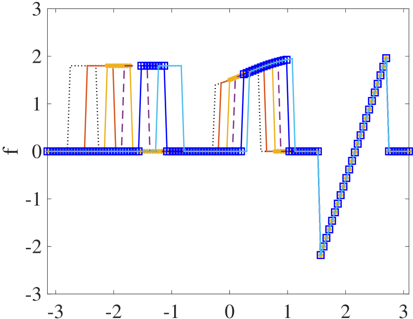
(a) $f_{j}$, $j=1,\dots,6$ in (38)

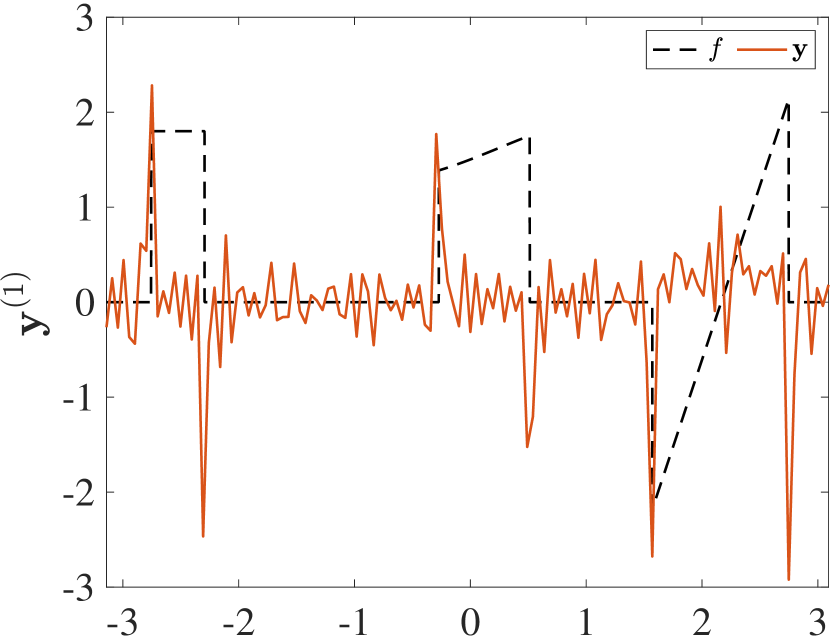
(b) $\bm{y}_{1}$

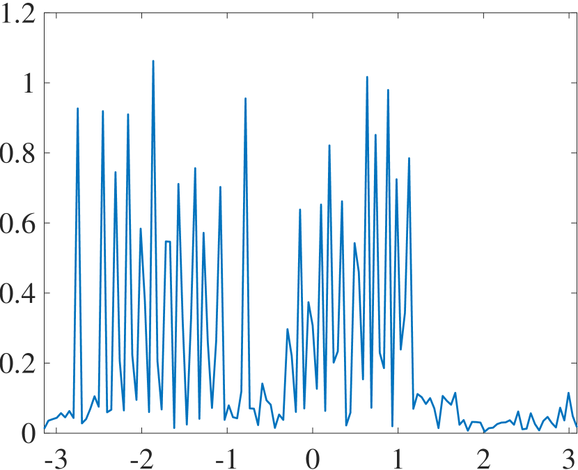
(c) The initialization of $\bm{q}$

Figure 1: (a) The sequence of functions given by Example 1. (b) $\bm{y}_{1}$ as defined in (9). (c) hyper-parameter $\bm{q}$ initialized in (30).

From Figure 1(c) we observe that the covariance matrix of the acquired data in (2) can roughly determine the interval in which the edge locations have moved. It is not very accurate, however, as there are spurious oscillations that affect the ability to determine the true shifted jump locations. Such a coarse initial estimate of the change region might be all that is available in a variety of applications, and indeed motivates our proposed framework here. That is, our method can still be useful even when the change region is not accurately described.

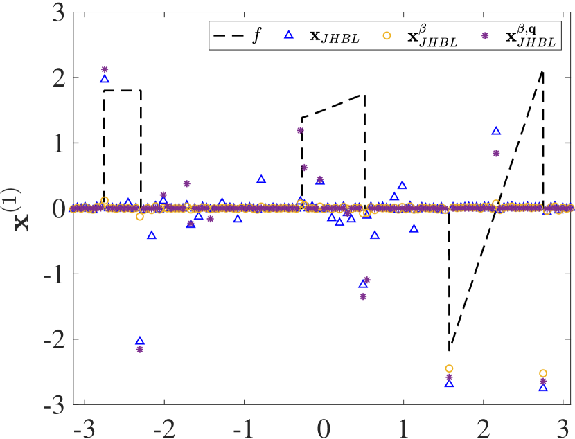
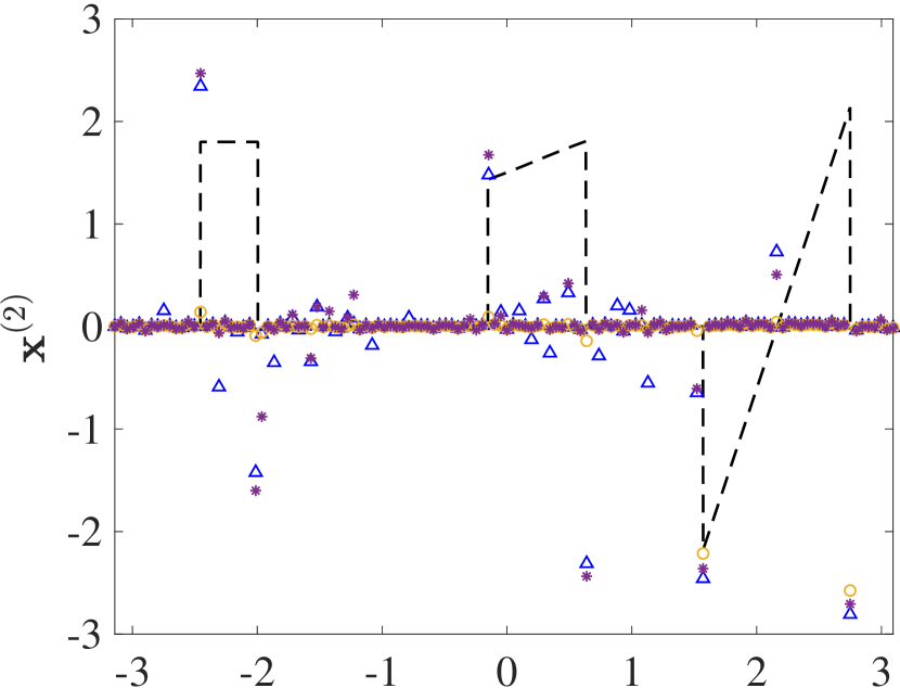
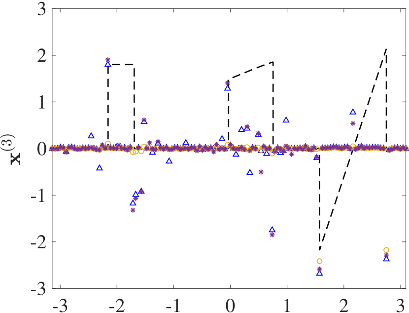
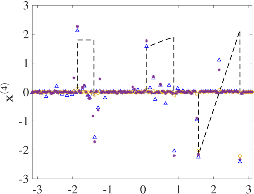
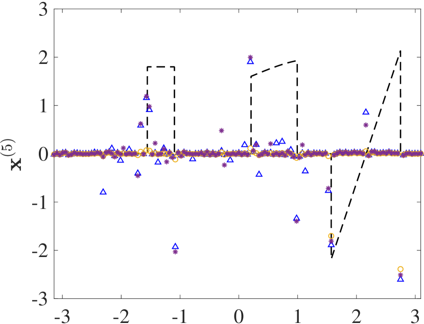
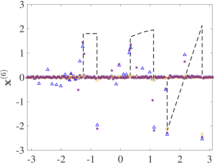
Figure 2: Sequential edge map recovery for Fourier measurements given by (39), $J=6$. The legend is provided in the top left figure.

Figure 2 compares the results of our new method to other existing approaches that seek to recover sparse signals from a sequence of given data. These include (1) $\bm{x}_{\operatorname{JHBL}}$, the JHBL recovery using Algorithm 2 with $\beta$ chosen a-priori and (2) $\bm{x}_{\operatorname{JHBL}}^{\beta}$, the JHBL recovery using Algorithm 1 for updating $\beta$ iteratively. We denote the results from our proposed method, realized using Algorithm 3, as $\bm{x}_{\operatorname{JHBL}}^{\beta,\bm{q}}$. We note that in our examples the exact value of $\beta$ is assumed for $\bm{x}_{\operatorname{JHBL}}$, but not for $\bm{x}_{\operatorname{JHBL}}^{\beta}$ or $\bm{x}_{\operatorname{JHBL}}^{\beta,\bm{q}}$. As can be observed from the results in Figure 2, by explicitly including change information, as is the main feature of Algorithm 3, we are able to more accurately capture the sequence of jump function recoveries. We used $\vartheta=0.05$ in (32) and note that some additional tuning may improve the results. More discussion regarding how parameter $\vartheta$ may be chosen follows (32).

Finally, we note that it is possible of course to use the standard SBL to recover the individual signals separately, that is without combining information from other data in the sequence. In this case the joint sparsity method is reduced to standard $\ell_{1}$ regularization (compressive sensing) given by (10). While the results for this simple example are comparable, we are interested in the problem where there is obstruction in each data acquisition that hampers individual recovery. For example, in our two-dimensional examples we consider the case where there are missing bands of Fourier data in each acquisition, so that no single acquisition has enough data to accurately recover the underlying image.

4.2 Two-dimensional data

Our two-dimensional examples include a magnetic resonance image (MRI) and a synthetic aperture radar (SAR) image. As was done for the one-dimensional sparse signal example, we also compare edge maps respectively recovered using Algorithm 1, Algorithm 2, and Algorithm 4. In contrast to the one-dimensional signal example, here we show how the temporal edge maps are employed for the downstream process of full image recovery.

Sequential mage recovery using edge maps

Since it pertains to the overall usefulness of our new sequential edge map recovery procedure, we now include a brief review of some commonly employed algorithms for sequential image recovery. Due to the sparsity in the edge domain, CS algorithms candes2006robust ; candes2006stable ; candes2006near ; donoho2006compressed are often employed to either separately (see e.g. above references) or jointly (see e.g. adcock2019jointsparsity ; cotter2005sparse ; chen2006theoretical ; eldar2009robust ; xiao2022sequential ) recover the corresponding sequence of images. For the standard single measurement case, the standard CS algorithm may be written as

$$\tilde{\bm{f}}_{j}=\operatorname*{arg\,min}_{\bm{f}^{\ast}}\left(\frac{1}{2}\mathinner{\!\left\lVert F_{j}\bm{f}^{\ast}-\tilde{\bm{g}}_{j}\right\rVert}_{2}^{2}+\lambda\mathinner{\!\left\lVert\mathcal{L}\bm{f}^{\ast}\right\rVert}_{1}\right),$$ (41)

where ${\mathcal{L}}$ is a sparsifying transform operator, designed here to promote sparsity in the edge domain. If the data acquisition model (4) is accurate, it should be the case that any measurement $\tilde{\bm{g}}_{j}$ carries sufficient information to recover its corresponding image so long as the regularization parameter is suitably chosen. The performance of CS algorithms deteriorate for seriously under-sampled data with low SNR, however, shchukina2017pitfalls ; kang2019compressive . Further, even if optimally chosen, the global impact of regularization term in (41) will make it impossible to resolve local features in these environments.

Spatially varying regularization parameters can improve the accuracy of the CS solution. Specifically, the parameter should be constructed to more heavily penalize the solution in the true sparse regions (in the edge domain) and less so in regions of presumed support. The (re-)weighted $\ell_{1}$ regularization method is designed for this purpose, with the most basic form written as candes2008enhancing

$$\tilde{\bm{f}}_{j}=\operatorname*{arg\,min}_{\bm{f}^{\ast}}\left(\frac{1}{2}\mathinner{\!\left\lVert F_{j}\bm{f}^{\ast}-\tilde{\bm{g}}_{j}\right\rVert}_{2}^{2}+\mathinner{\!\left\lVert W\mathcal{L}\bm{f}^{\ast}\right\rVert}_{1}\right).$$ (42)

Here the entries $\bm{w}_{j}$ of the diagonal weighting matrix $W=\operatorname{diag}{(\bm{w}_{j})}$ typically are iteratively constructed, yielding expensive computational cost. Furthermore, errors in $W$ due to noise and incompleteness of acquired data will be fed into (42) and the resulting error will propagate at each iteration.

As the edge information of each part of the temporal sequence has been determined prior to the image reconstruction, following what was done in adcock2019jointsparsity ; gelb2019reducing ; scarnati2019accelerated , we avoid iterating on $W$ and define a pre-computed weighting matrix as

$$\omega^{(j)}(i)=\frac{1}{\text{vec}\left(\tilde{\bm{x}}_{j}\right)(i)+\epsilon},$$ (43)

where $\text{vec}(\cdot)$ is to stack input vertically as a vector and $\epsilon=10^{-4}$ is introduced to avoid zero-valued denominator. We further scale the matrix with maximum value 1 and replace (43) as

$$\omega^{(j)}(i)=\frac{\omega^{(j)}(i)}{\max_{i}{\mathinner{\!\left\lvert\omega^{(j)}(i)\right\rvert}}}.$$ (44)

We follow gelb2019reducing and employ the Alternating Direction Method of Multipliers (ADMM) (see boyd2011distributed ), to solve the convex optimization problem in (42).

Sequential MRI

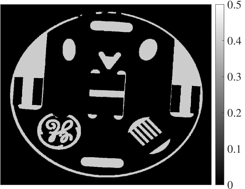
(a) $\bm{f}_{1}$

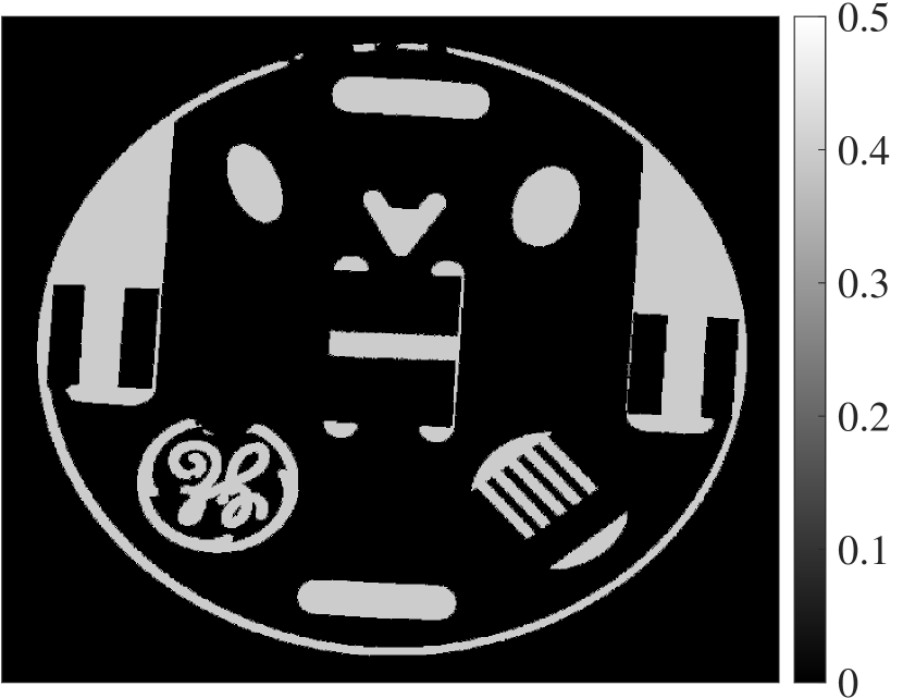
(b) $\bm{f}_{2}$

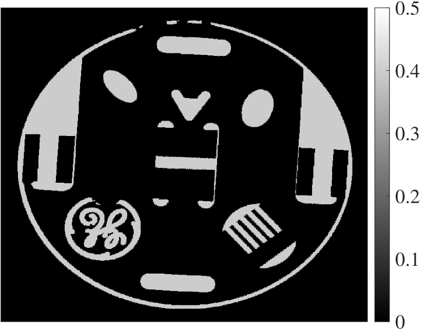
(c) $\bm{f}_{3}$

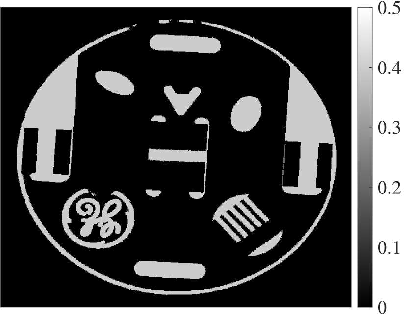
(d) $\bm{f}_{4}$

(e) $\bm{x}_{1}$

(f) $\bm{x}_{2}$

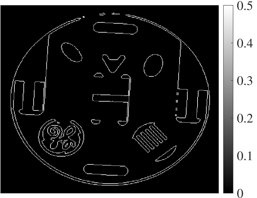
(g) $\bm{x}_{3}$

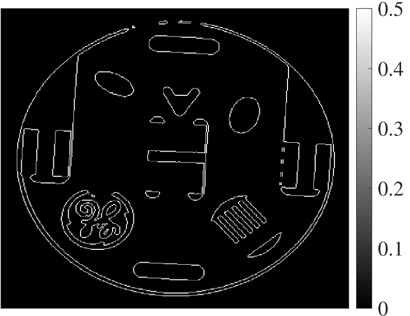
(h) $\bm{x}_{4}$

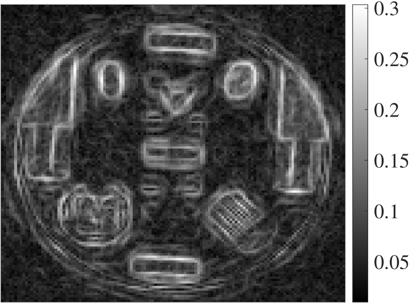
(i) $\mathbf{y}_{1}$

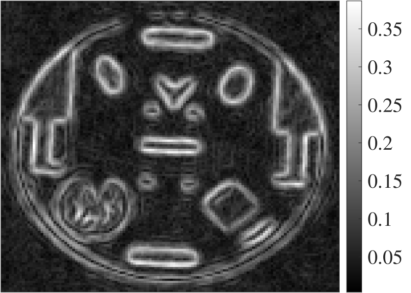
(j) $\mathbf{y}_{2}$

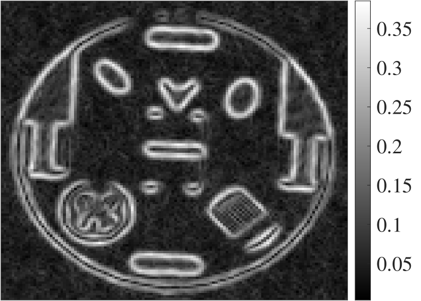
(k) $\mathbf{y}_{3}$

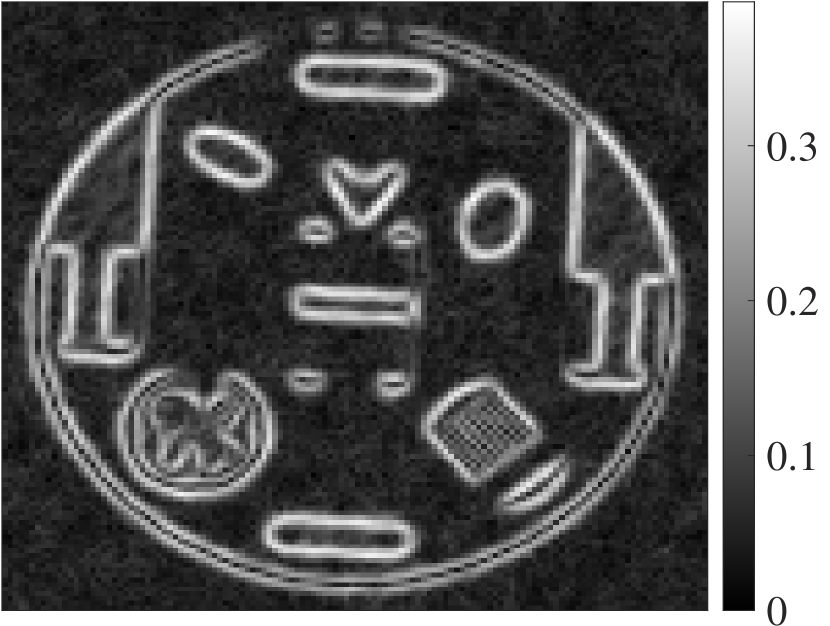
(l) $\mathbf{y}_{4}$

Figure 3: (top row) The underlying MRI images, Lalwanietal . Two rotating/translating ellipses are imposed on each image. (middle row) The exact edge map for each MRI image. (bottom row) The edge approximations using the two-dimensional extension of the CF method (7) (see e.g. xiao2022sequential ) from the under-sampled and noisy Fourier samples. Here we use SNR $=2$ for the noise standard deviation in (40).

Figure 3(top) shows four sequential MRI images. Two ellipses that are rotating/translating in time are super-imposed on each static image. We assume we are given the corresponding Fourier data for $J=6$ (with four shown for better visualization) sequential images, which we simulate by taking the discrete Fourier transform of each $128\times 128$ pixelated image. We also “zero out” a symmetric band $\mathcal{K}_{j}$, $j=1,\dots,J$, given by

$$\mathcal{K}_{j}=[\pm(10j+1),\pm(10(j+1))],$$ (45)

and then add noise with SNR $=2$. The intervals for the missing data bands were somewhat arbitrarily chosen, with the idea being that in each case relevant information in each data set of the sequence would be compromised in some way. Figure 3(middle) shows the exact edge map at each time, while Figure 3(bottom) displays the edge maps obtained using the two-dimensional expansion of the CF method in (7) (see e.g. adcock2019jointsparsity ; gelb2017detecting ; xiao2022sequential for discussion on two-dimensional CF method expansion).

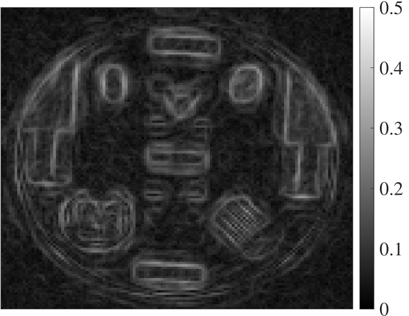
(a) ${\bm{x}_{1}}_{\operatorname{JHBL}}$

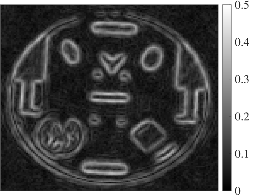
(b) ${\bm{x}_{2}}_{\operatorname{JHBL}}$

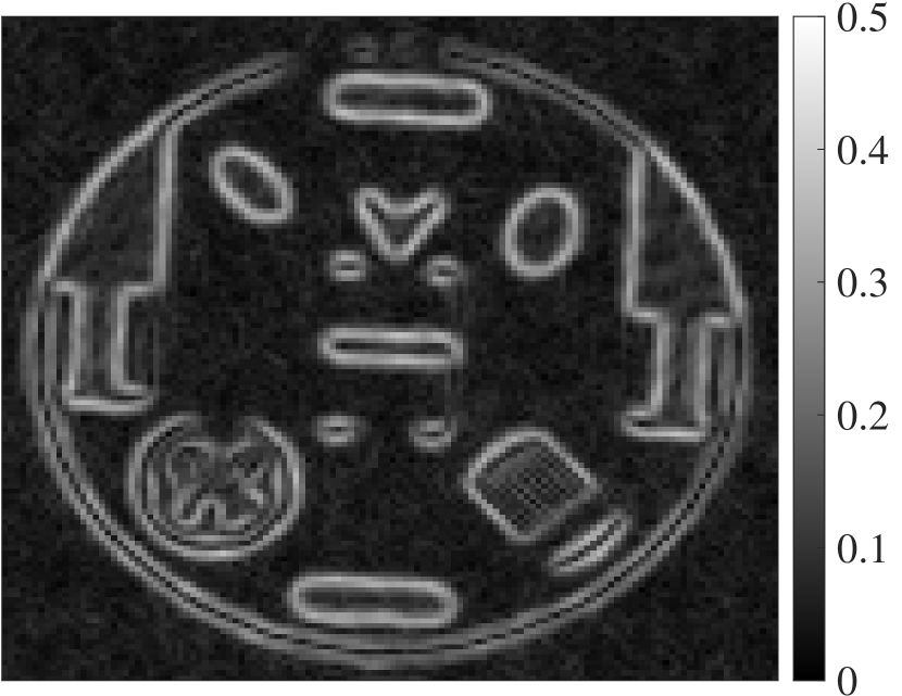
(c) ${\bm{x}_{3}}_{\operatorname{JHBL}}$

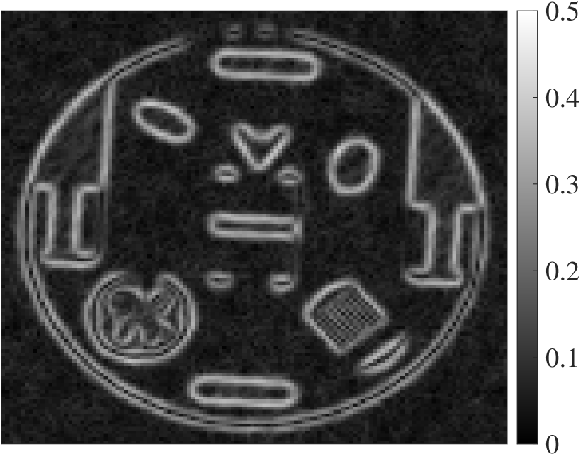
(d) ${\bm{x}_{4}}_{\operatorname{JHBL}}$

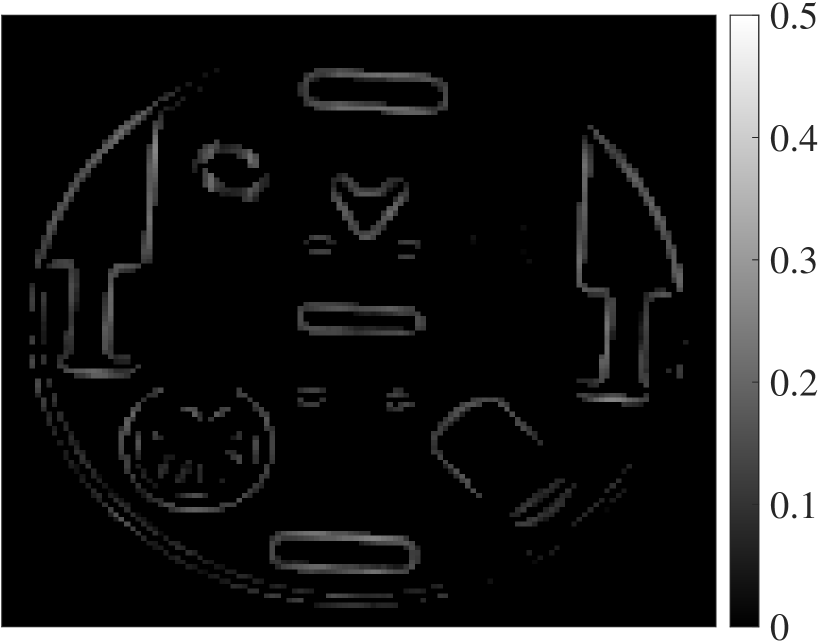
(e) ${\bm{x}_{1}}^{\beta}_{\operatorname{JHBL}}$

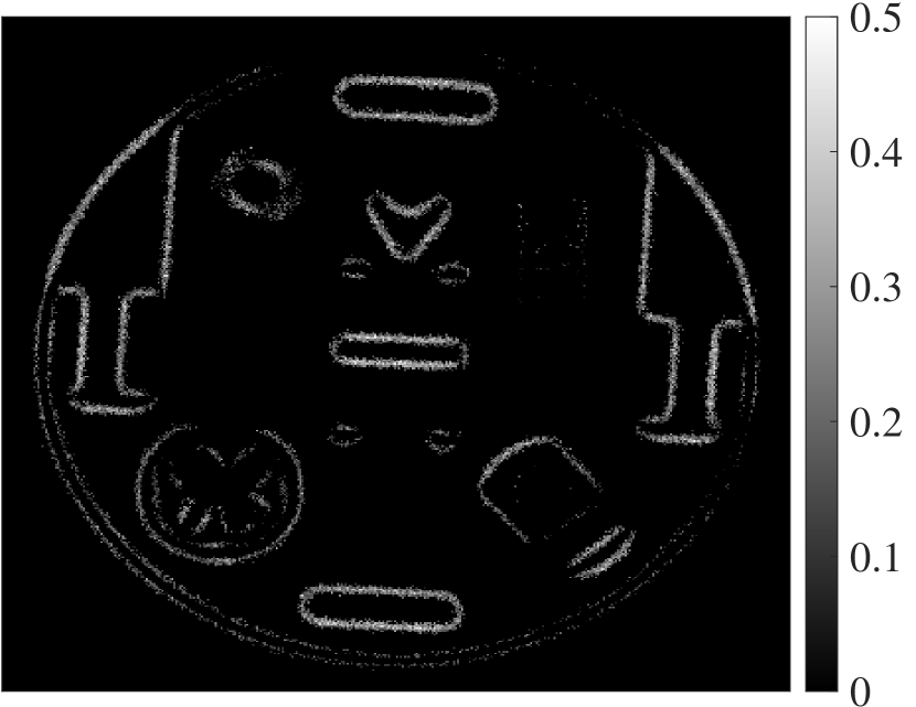
(f) ${\bm{x}_{2}}^{\beta}_{\operatorname{JHBL}}$

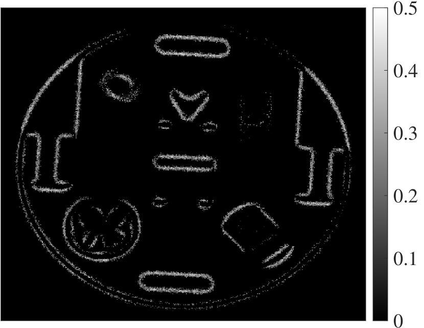
(g) ${\bm{x}_{3}}^{\beta}_{\operatorname{JHBL}}$

(h) ${\bm{x}_{4}}^{\beta}_{\operatorname{JHBL}}$

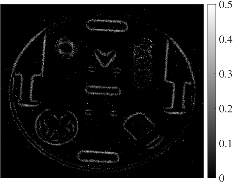
(i) ${\bm{x}_{1}}^{\beta,\bm{q}}_{\operatorname{JHBL}}$

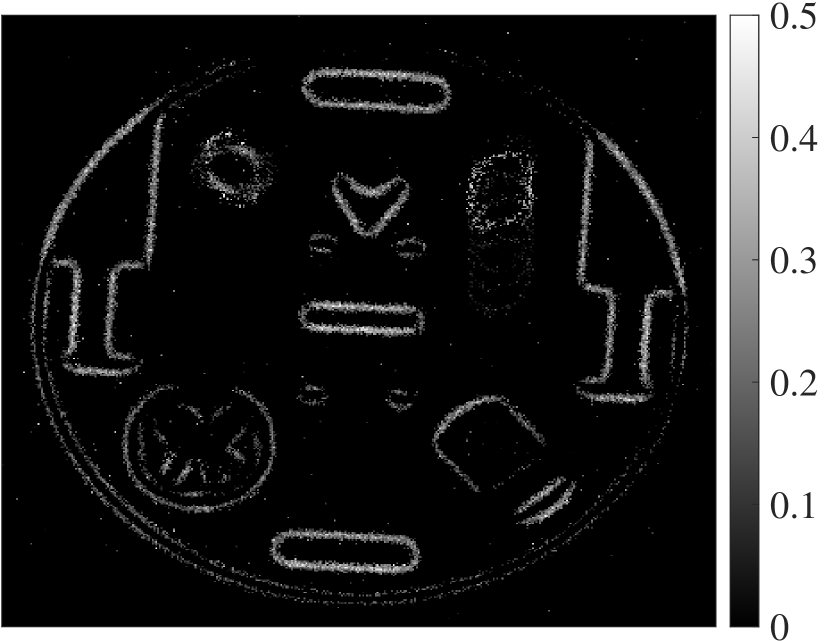
(j) ${\bm{x}_{2}}^{\beta,\bm{q}}_{\operatorname{JHBL}}$

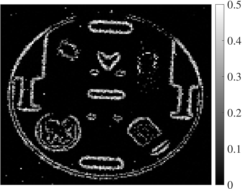
(k) ${\bm{x}_{3}}^{\beta,\bm{q}}_{\operatorname{JHBL}}$

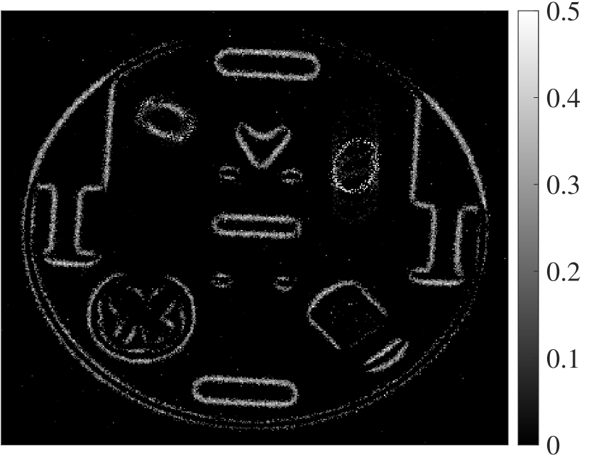
(l) ${\bm{x}_{4}}^{\beta,\bm{q}}_{\operatorname{JHBL}}$

Figure 4: (top row) Edge map recovery using Algorithm 2. (middle row) Edge map recovery using Algorithm 1. (bottom row) Edge map recovery using Algorithm 4.

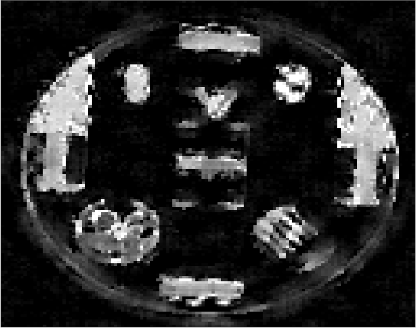
(a) ${\bm{x}_{1}}_{\operatorname{JHBL}}$

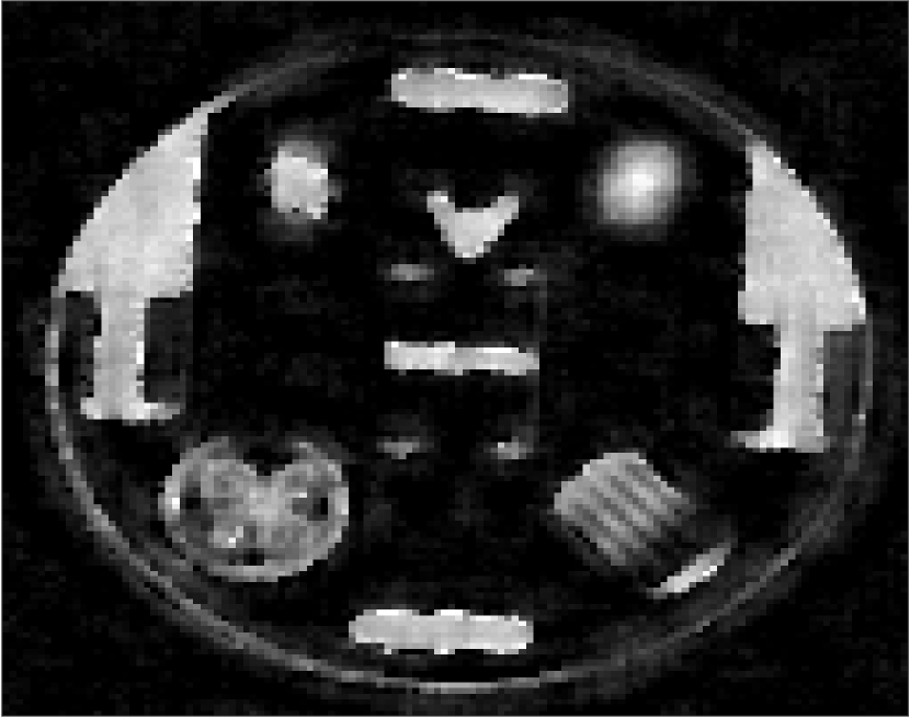
(b) ${\bm{x}_{1}}^{\beta}_{\operatorname{JHBL}}$

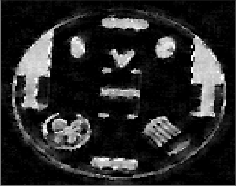
(c) ${\bm{x}_{1}}^{\beta,\bm{q}}_{\operatorname{JHBL}}$

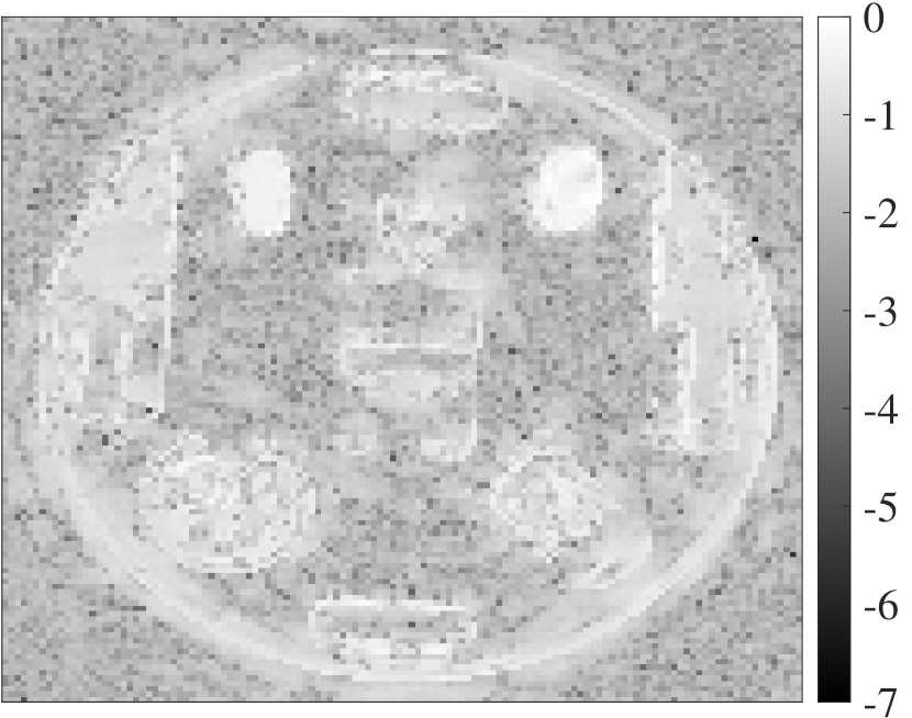
(d) ${\bm{x}_{1}}_{\operatorname{JHBL}}$

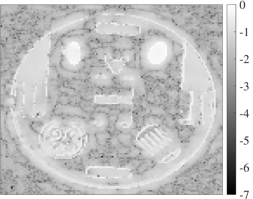
(e) ${\bm{x}_{1}}^{\beta}_{\operatorname{JHBL}}$

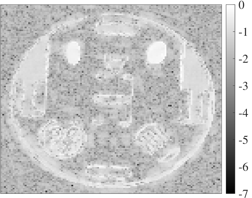
(f) ${\bm{x}_{1}}^{\beta,\bm{q}}_{\operatorname{JHBL}}$

Figure 5: (top) Image recovery of the first image in the sequence via (42) with weights informed by (left) Algorithm 2; (middle) Algorithm 1; and (right) Algorithm 4. (bottom) The corresponding log-scale pointwise error.

Figure 4 compares edge recovery using the JHBL method given by Algorithm 2, which assumes information regarding $\beta$ is known a-priori, the standard JHBL method, given by Algorithm 1, which learns $\beta$ but does not refine the parameters based on inter-signal information, and Algorithm 4, which refines the parameter selection by accounting for both intra- and inter-image information at each of the four time instances, again based on $J=6$ original data sets. It is evident that which band is missing (45) plays an important role in how well each method is able to resolve the edges. Using a priori information regarding $\beta$ so that $\beta=\frac{1}{\sigma^{2}}$, (top row) captures the internal structures but appears to result in additional clutter. Learning $\beta$ without refining the hyperparameters according to inter-signal information results in loss of moving edge information in each recovered edge map (second row). In all cases, refining ${\bm{q}}$ improves resolution while mitigating the effects of both the corrupted data and the change of support locations in the edge domain (bottom row). For this example we chose $\vartheta=0.3$ in (37) and note that some additional tuning may improve the results.

We observe in particular the poor edge map recovery quality using the JHBL approach with fixed $\ignorespaces\beta$ (Algorithm 2) in the first column of the first row in Figure 4, which is likely due to the zeroed out low frequencies in (45). In the middle row, we see that while the stationary edge map structures are recovered more accurately, the changed regions are not retrieved in the update process used by Algorithm 1. By contrast, our new approach in Algorithm 4 is able both to enhance the quality observed when using Algorithm 2 while also recovering the changed regions in the edge maps (bottom row).

Figure 5 demonstrates how the edge maps from each recovery can be used to inform the weights in (44) which is in turn used in the weighted $\ell_{1}$ regularization method given by (42) for image recovery. While only the first image in the sequence is displayed, the results for the rest of the sequence are comparable. In particular we observe that using Algorithm 4 consistently performs as well as or better than the other two edge recovery methods which do not properly account for change information. It is also once again evident that which band is missing (45) plays an important role in how well each method is able to resolve the features in each image.

Sequential SAR images

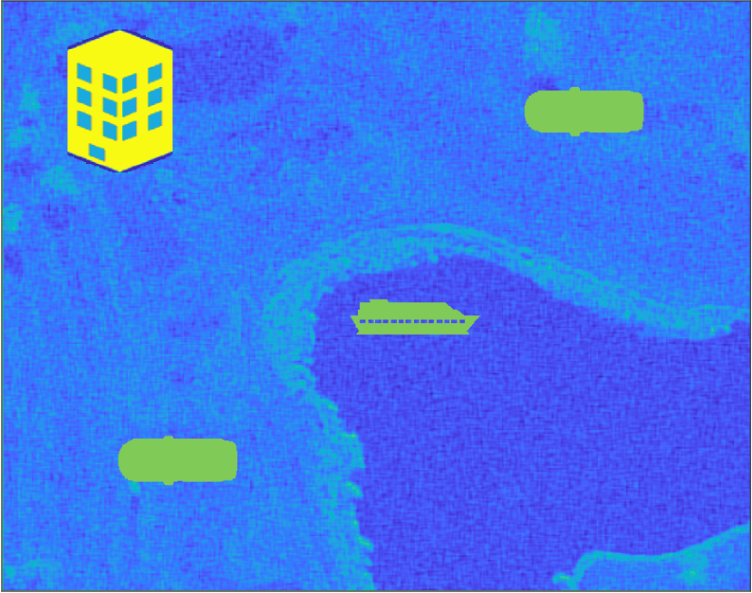
(a) $\bm{f}_{1}$

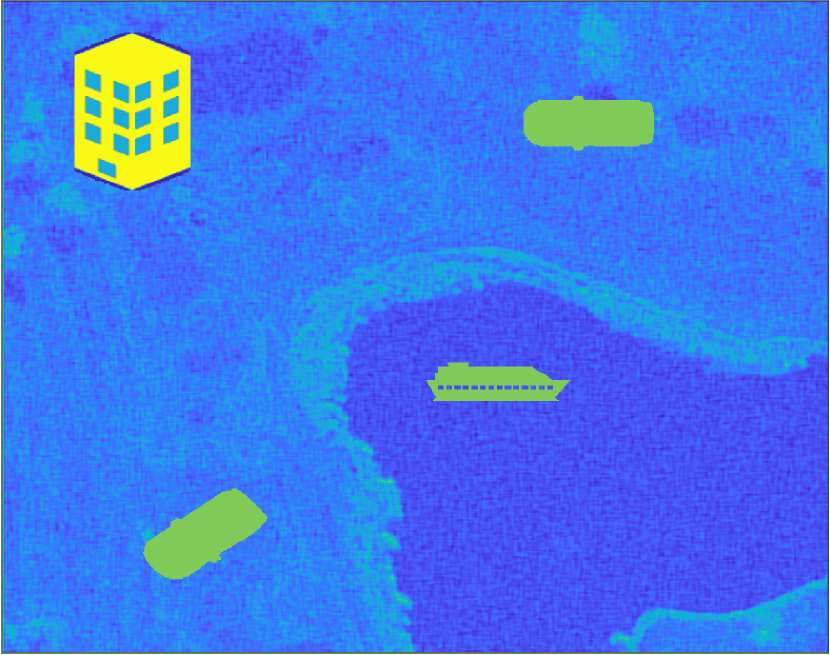
(b) $\bm{f}_{2}$

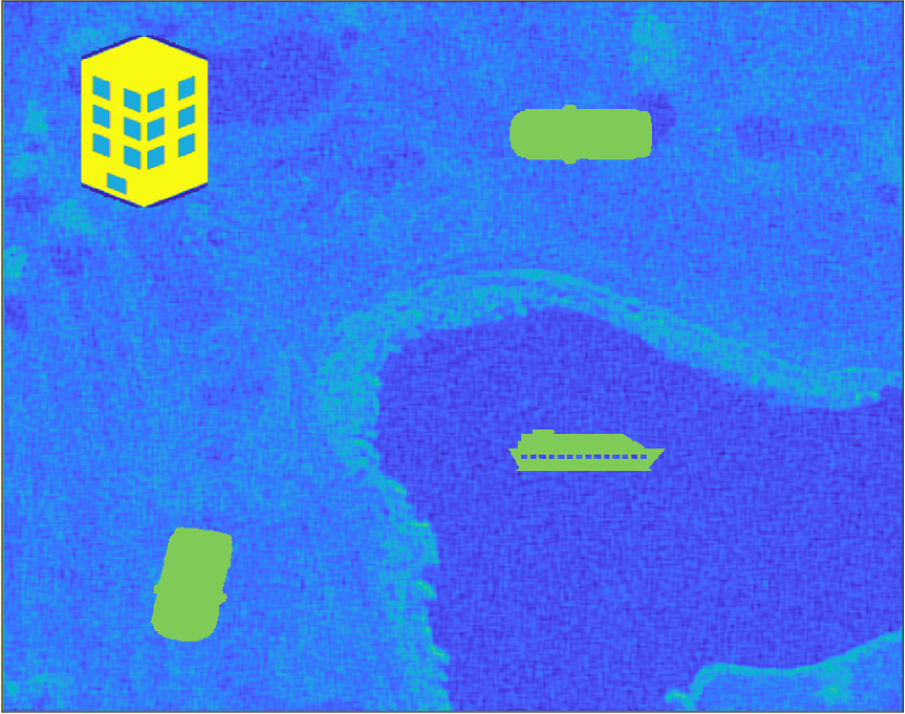
(c) $\bm{f}_{3}$

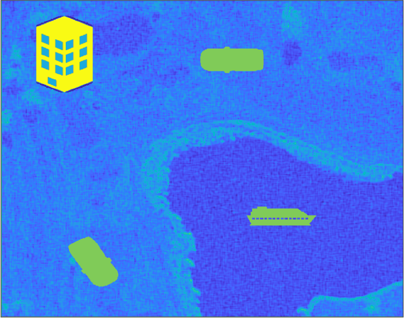
(d) $\bm{f}_{4}$

Figure 6: The underlying scene is the SAR image of a golf course, SAR_Image_ref , with a superimposed (static) hotel, and translating/rotating cars and boats.

For the second experiment we consider a temporal sequence of six SAR images of a golf course, SAR_Image_ref , four of which are displayed in Figure 6. Observe there is no “ground truth” in this case. As in the MRI case, we again use the discrete Fourier transform of the $128\times 128$ pixelated image to obtain the measurement data. We once again assume a symmetric band of measurements, $\{\mathcal{K}_{j}\}_{j=1}^{J}$ given in (45), is for some reason not available for use. Finally, we add noise with SNR $=2$.

To respectively simulate moving and background objects, we impose cars and boats on the scene, each of magnitude $1$, and a building of magnitude $1.5$.

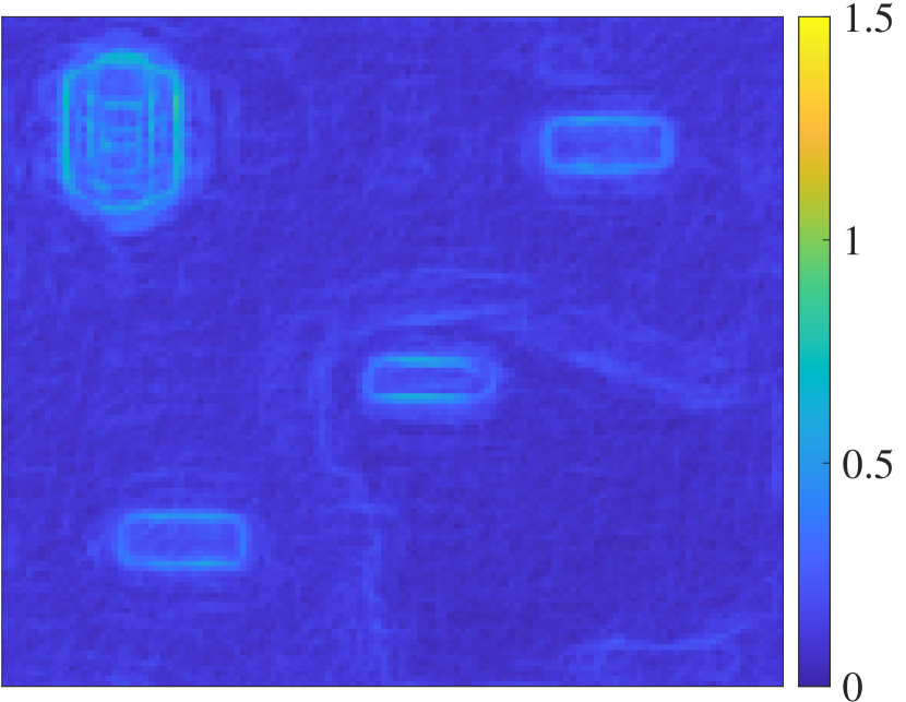
(a) ${\bm{x}_{1}}_{\operatorname{JHBL}}$

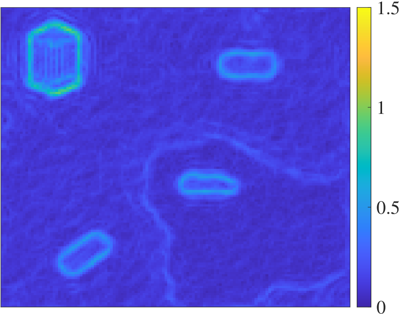
(b) ${\bm{x}_{2}}_{\operatorname{JHBL}}$

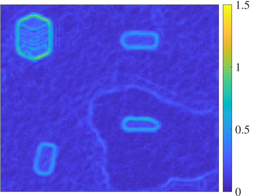
(c) ${\bm{x}_{3}}_{\operatorname{JHBL}}$

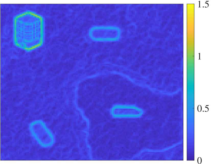
(d) ${\bm{x}_{4}}_{\operatorname{JHBL}}$

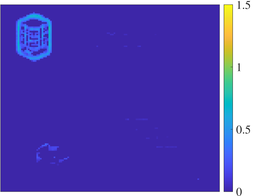
(e) ${\bm{x}_{1}}^{\beta}_{\operatorname{JHBL}}$

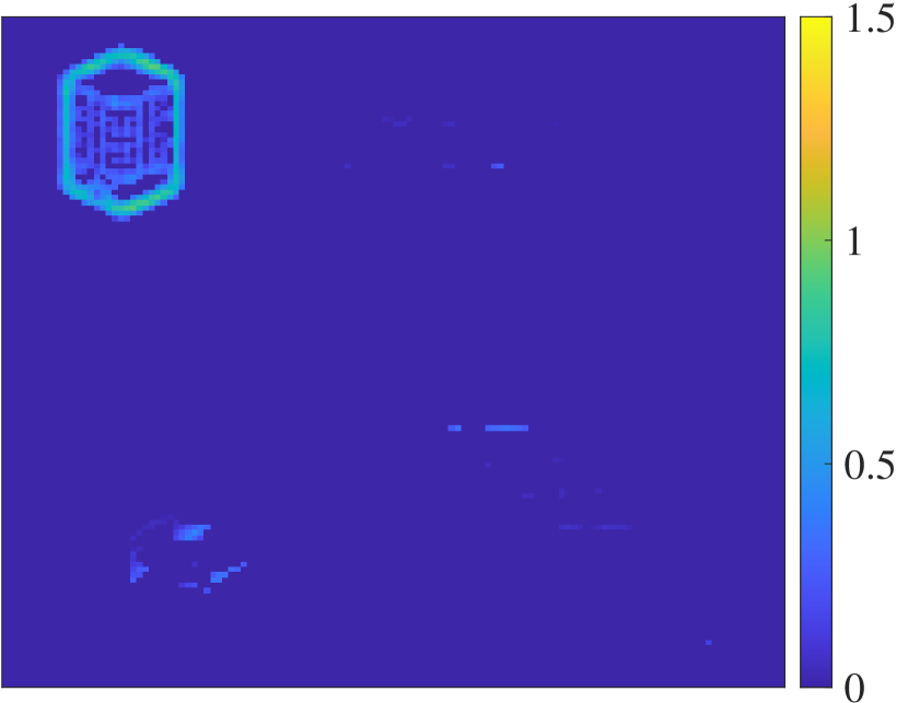
(f) ${\bm{x}_{2}}^{\beta}_{\operatorname{JHBL}}$

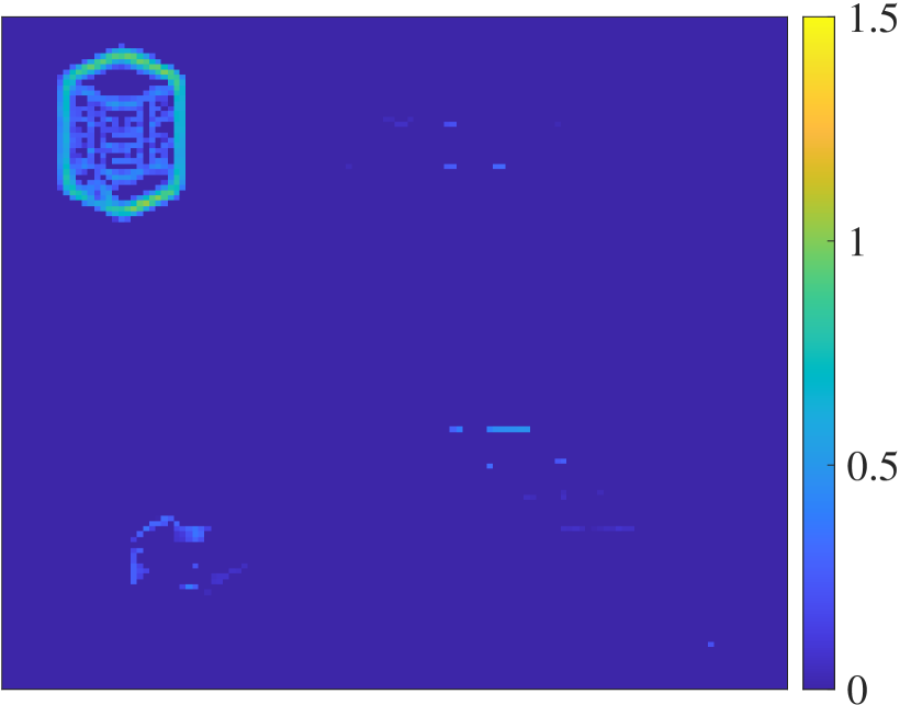
(g) ${\bm{x}_{3}}^{\beta}_{\operatorname{JHBL}}$

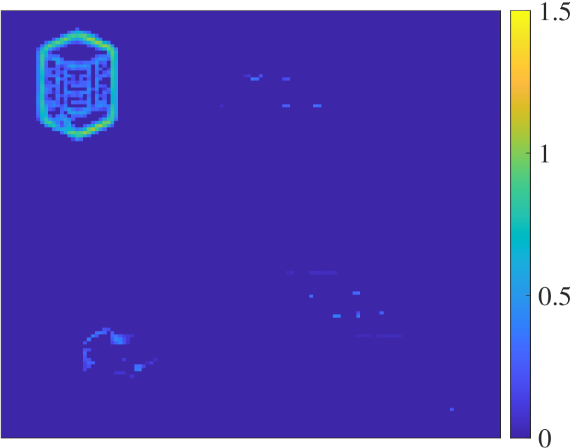
(h) ${\bm{x}_{4}}^{\beta}_{\operatorname{JHBL}}$

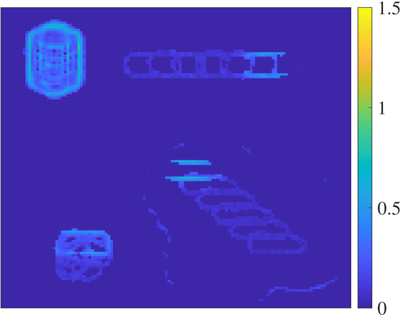
(i) ${\bm{x}_{1}}^{\beta,\bm{q}}_{\operatorname{JHBL}}$

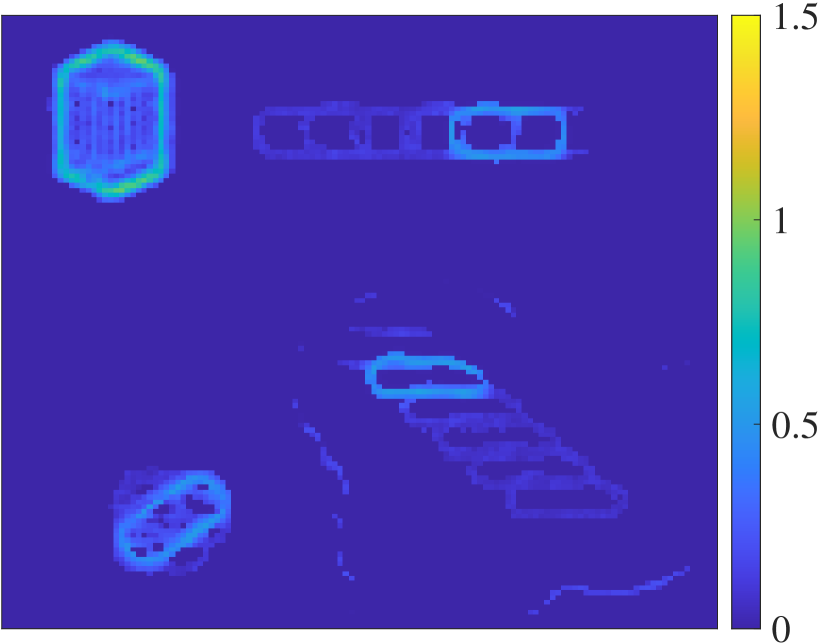
(j) ${\bm{x}_{2}}^{\beta,\bm{q}}_{\operatorname{JHBL}}$

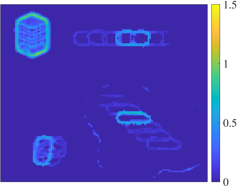
(k) ${\bm{x}_{3}}^{\beta,\bm{q}}_{\operatorname{JHBL}}$

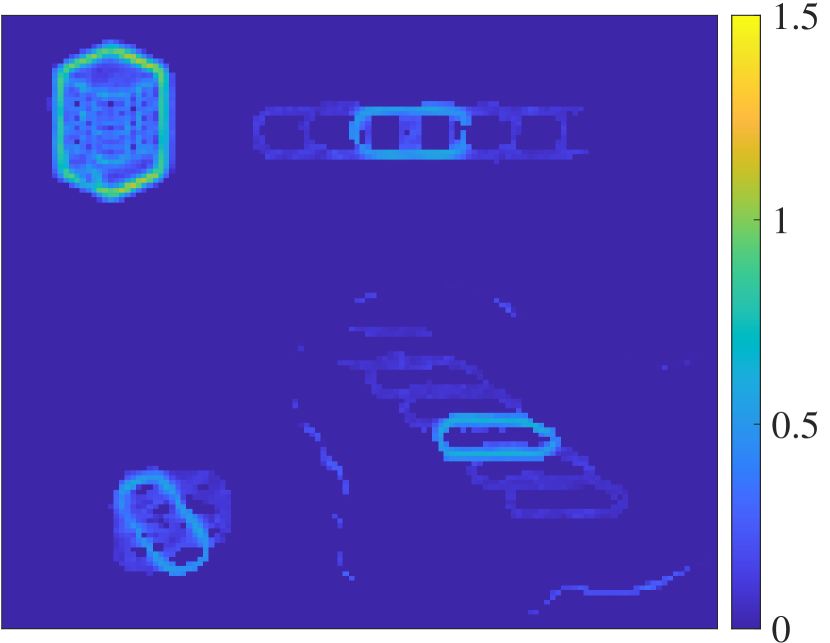
(l) ${\bm{x}_{4}}^{\beta,\bm{q}}_{\operatorname{JHBL}}$

Figure 7: Sequential edge map recovery shown at four time stamps using (top) Algorithm 2; (middle) Algorithm 1; and (bottom) Algorithm 4.

As in the sequential MRI example, we first compare edge map recoveries using the different algorithms in Figure 7. The edges are then used to inform the weights in (44) for the weighted $\ell_{1}$ regularization method (42). Figure 8 displays the results for the fourth image in the sequence. The results for the rest of the sequence are similar. Overall, it is clear that by using Algorithm 4 we are more able to capture the structural details in the underlying images without “oversmoothing” the background. We note that using either Algorithm 1 or Algorithm 2 is sufficient for obtaining weights in (42) for some images in the sequence, however the results are not consistent.

More distinction between the results of each algorithm are observed in the sequential edge map recovery. Figure 7 shows cluttering in the edge maps when using Algorithm 2. Learning the hyperparameters without the benefit of correlating temporal information (Algorithm 1) reduces the clutter, but as was the case for the MRI example, the rotating and translating structures are lost. Only Algorithm4, which refines the hyperparameters to consider inter-signal correlations is able to capture moving objects.

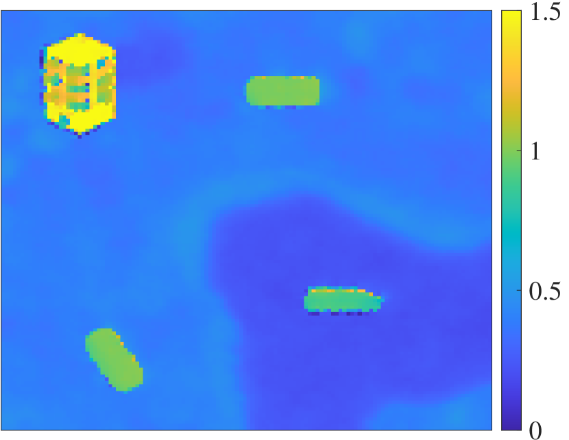
(a) ${\bm{x}_{4}}_{\operatorname{JHBL}}$

(b) ${\bm{x}_{4}}^{\beta}_{\operatorname{JHBL}}$

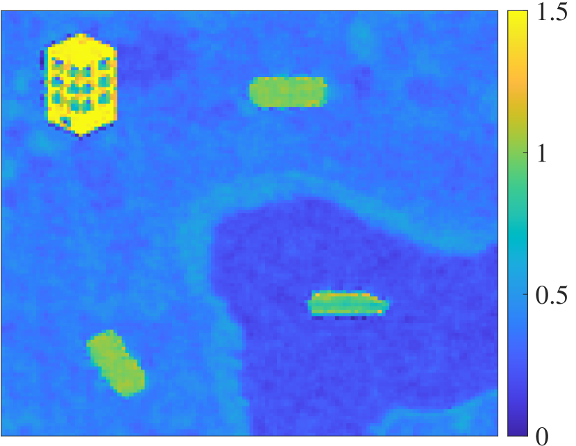
(c) ${\bm{x}_{4}}^{\beta,\bm{q}}_{\operatorname{JHBL}}$

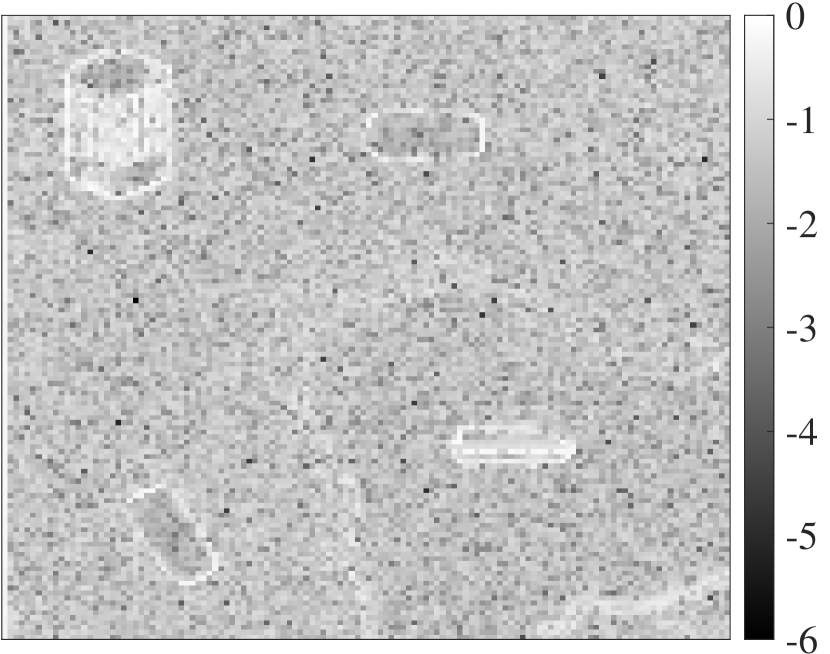
(d) ${\bm{x}_{4}}_{\operatorname{JHBL}}$

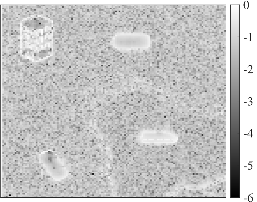
(e) ${\bm{x}_{4}}^{\beta}_{\operatorname{JHBL}}$

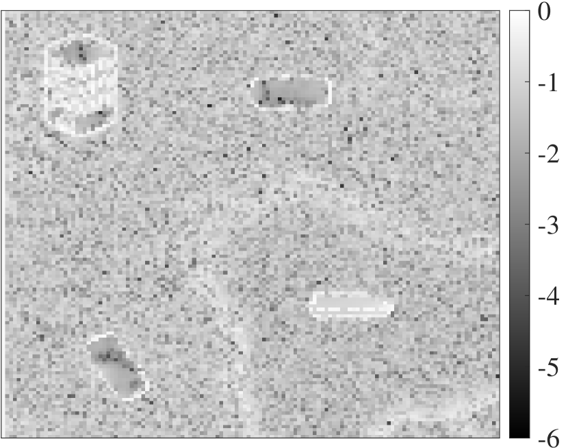
(f) ${\bm{x}_{4}}^{\beta,\bm{q}}_{\operatorname{JHBL}}$

Figure 8: (top row) Image recovery using (42) where the weights are informed by (left) Algorithm 2 (middle) Algorithm 1 and (right) Algorithm 4. (bottom row) The corresponding log-scale pointwise error of the images in the top row.

5 Conclusion

In this paper we proposed a new sparse Bayesian learning algorithm to jointly recover a temporal sequence of edge maps from under-sampled and noisy Fourier data of piecewise smooth functions and images. Since each data set in the temporal sequence only acquires partial information regarding the underlying scene, it is not possible to individually recover each edge map in the sequence. Our new method incorporates both inter- and intra-image information into the design of the prior distribution. This is in contrast to standard multiple-measurement SBL approaches, which require stationary support across the temporal sequence. Moreover, unlike the deterministic method developed in xiao2022sequential , our approach does not require the explicit construction of sequential change masks, which adds numerical cost as well as introduces more parameters.

Our new algorithm compares favorably to more standard SBL approaches in regions where the underlying function is smooth (correspondingly zero in the jump function). In particular we observed in our one-dimensional example that fewer non-zero values were returned in smooth regions where the data sequence share the joint sparsity profile. Furthermore, our new method does not suffer as much magnitude loss at the true (non-zero) jump locations. The magnitudes at varied jump locations (across the sequence) are also much more accurate using our method, although there are some oscillations in the surrounding neighborhoods. By contrast, we observed that jump locations were completely missed when the hyperparameters were not temporally correlated.

While these initial results are promising, our method should be refined for more complicated sequences of images. For example, an empirical method can be introduced to determine the shape and rate of hyper-parameters for the partial joint support of the temporal data stream. This would potentially involve another layer of hyper-hyper-parameters in the hierarchical Bayesian structure. Similarly, the proposed framework can be applied to complex-valued signals (or images), where there is sparsity in the magnitude of the signal. This would be important in SAR or ultrasound images. We anticipate using sampling techniques such as Markov chain Monte Carlo (MCMC) and Gibbs sampling in these cases which will also allow uncertainty quantification of the solution posterior.

Data Availability All underlying data sets can be made available upon request or are publicly available. MATLAB codes used for obtaining results is available upon request to the authors. MRI GE images were originally publicly provided by researchers at the Barrow Neurological Institute for the purpose of algorithmic development. The SAR golf course image is provided in SAR_Image_ref .

Acknowledgments

This work is partially supported by the NSF grants DMS #1912685 (AG), DMS #1939203 (GS), AFOSR grant #FA9550-22-1-0411 (AG), DOE ASCR #DE-ACO5-000R22725 (AG), and ONR MURI grant #N00014-20-1-2595 (AG).

References

- (1) Adcock, B., Gelb, A., Song, G., Sui, Y.: Joint sparse recovery based on variances. SIAM Journal of Scientific Computing 41(1), A246–A268 (2019). 10.1137/17M1155983
- (2) Archibald, R., Gelb, A., Platte, R.B.: Image reconstruction from undersampled Fourier data using the polynomial annihilation transform. Journal of Scientific Computing 67(2), 432–452 (2016)
- (3) Artin, E.: The gamma function. Courier Dover Publications (2015)
- (4) Azzali, S., Menenti, M.: Mapping vegetation-soil-climate complexes in southern Africa using temporal Fourier analysis of NOAA-AVHRR NDVI data. International Journal of Remote Sensing 21(5), 973–996 (2000)
- (5) Bardsley, J.M.: MCMC-based image reconstruction with uncertainty quantification. SIAM Journal on Scientific Computing 34(3), A1316–A1332 (2012)
- (6) Boyd, S., Parikh, N., Chu, E.: Distributed optimization and statistical learning via the alternating direction method of multipliers (2011). 10.1561/2200000016
- (7) Calvetti, D., Pragiola, M., Somersalo, E.: Hybrid solver for hierarchical Bayesian inverse problems. arXiv preprint arXiv:2003.06532 (2020)
- (8) Calvetti, D., Pragliola, M., Somersalo, E.: Sparsity promoting hybrid solvers for hierarchical Bayesian inverse problems. SIAM Journal on Scientific Computing 42(6), A3761–A3784 (2020)
- (9) Calvetti, D., Pragliola, M., Somersalo, E., Strang, A.: Sparse reconstructions from few noisy data: analysis of hierarchical Bayesian models with generalized gamma hyperpriors. Inverse Problems 36(2), 025010 (2020)
- (10) Calvetti, D., Somersalo, E.: An introduction to Bayesian scientific computing: ten lectures on subjective computing, vol. 2. Springer Science & Business Media (2007)
- (11) Calvetti, D., Somersalo, E., Strang, A.: Hierachical Bayesian models and sparsity: -magic. Inverse Problems 35(3), 035003 (2019)
- (12) Candès, E.J., Romberg, J., Tao, T.: Robust uncertainty principles: Exact signal reconstruction from highly incomplete frequency information. IEEE Transactions on information theory 52(2), 489–509 (2006)
- (13) Candès, E.J., Romberg, J.K., Tao, T.: Stable signal recovery from incomplete and inaccurate measurements. Communications on Pure and Applied Mathematics: A Journal Issued by the Courant Institute of Mathematical Sciences 59(8), 1207–1223 (2006)
- (14) Candès, E.J., Tao, T.: Near-optimal signal recovery from random projections: Universal encoding strategies? IEEE transactions on information theory 52(12), 5406–5425 (2006)
- (15) Candès, E.J., Wakin, M.B., Boyd, S.P.: Enhancing sparsity by reweighted minimization. Journal of Fourier analysis and applications 14(5), 877–905 (2008)
- (16) Cetin, M., Moses, R.L.: SAR imaging from partial-aperture data with frequency-band omissions. In: Defense and Security, pp. 32–43. International Society for Optics and Photonics (2005)
- (17) Çetin, M., Stojanović, I., Önhon, N.Ö., Varshney, K., Samadi, S., Karl, W.C., Willsky, A.S.: Sparsity-driven synthetic aperture radar imaging: Reconstruction, autofocusing, moving targets, and compressed sensing. IEEE Signal Processing Magazine 31(4), 27–40 (2014)
- (18) Chen, J., Huo, X.: Theoretical results on sparse representations of multiple-measurement vectors. IEEE Transactions on Signal processing 54(12), 4634–4643 (2006)
- (19) Chen, W., Wipf, D., Wang, Y., Liu, Y., Wassell, I.J.: Simultaneous bayesian sparse approximation with structured sparse models. IEEE Transactions on Signal Processing 64(23), 6145–6159 (2016)
- (20) Churchill, V., Archibald, R., Gelb, A.: Edge-adaptive regularization image reconstruction from non-uniform Fourier data. Inverse Problems and Imaging 13(5), 931–958 (2019)
- (21) Cotter, S.F., Rao, B.D., Engan, K., Kreutz-Delgado, K.: Sparse solutions to linear inverse problems with multiple measurement vectors. IEEE Transactions on Signal Processing 53(7), 2477–2488 (2005)
- (22) Dempster, A.P., Laird, N.M., Rubin, D.B.: Maximum likelihood from incomplete data via the EM algorithm. Journal of the Royal Statistical Society: Series B (Methodological) 39(1), 1–22 (1977)
- (23) Deng, W., Yin, W., Zhang, Y.: Group sparse optimization by alternating direction method. In: Wavelets and Sparsity XV, vol. 8858, pp. 242–256. SPIE (2013)
- (24) Donoho, D.L.: Compressed sensing. IEEE Transactions on information theory 52(4), 1289–1306 (2006)
- (25) Eldar, Y.C., Mishali, M.: Robust recovery of signals from a structured union of subspaces. IEEE Transactions on Information Theory 55(11), 5302–5316 (2009)
- (26) Ellsworth, M., Thomas, C.: A fast algorithm for image deblurring with total variation regularization. Unmanned Tech Solutions 4 (2014)
- (27) Fergus, R., Singh, B., Hertzmann, A., Roweis, S.T., Freeman, W.T.: Removing camera shake from a single photograph. In: ACM SIGGRAPH 2006 Papers, pp. 787–794 (2006)
- (28) Figueiredo, M.A., Bioucas-Dias, J.M., Nowak, R.D.: Majorization–minimization algorithms for wavelet-based image restoration. IEEE Transactions on Image processing 16(12), 2980–2991 (2007)
- (29) Gelb, A., Scarnati, T.: Reducing effects of bad data using variance based joint sparsity recovery. Journal of Scientific Computing 78(1), 94–120 (2019)
- (30) Gelb, A., Song, G.: Detecting edges from non-uniform Fourier data using Fourier frames. Journal of Scientific Computing 71(2), 737–758 (2017)
- (31) Gelb, A., Song, G.: Detecting edges from non-uniform Fourier data using Fourier frames. J. Sci. Comput. 71(2), 737–758 (2017)
- (32) Gelb, A., Tadmor, E.: Detection of edges in spectral data. Applied and computational harmonic Analysis 7(1), 101–135 (1999)
- (33) Gelb, A., Tadmor, E.: Detection of edges in spectral data II. Nonlinear enhancement. SIAM Journal on Numerical Analysis 38(4), 1389–1408 (2000)
- (34) Gelman, A., Carlin, J.B., Stern, H.S., Dunson, D.B., Vehtari, A., Rubin, D.B.: Bayesian Data Analysis, third edn. Chapman and Hall/CRC, New York (2015). 10.1201/b16018
- (35) Glaubitz, J., Gelb, A., Song, G.: Generalized sparse bayesian learning and application to image reconstruction. arXiv preprint arXiv:2201.07061 (2022)
- (36) Jakowatz, C.V., Wahl, D.E., Eichel, P.H., Ghiglia, D.C., Thompson, P.A.: Spotlight-mode synthetic aperture radar: A signal processing approach. Springer Science & Business Media (2012)
- (37) Kaipio, J., Somersalo, E.: Statistical and Computational Inverse Problems. Applied Mathematical Sciences. Springer New York (2006). URL https://books.google.com.hk/books?id=h0i-Gi4rCZIC
- (38) Kang, M.S., Kim, K.T.: Compressive sensing based SAR imaging and autofocus using improved Tikhonov regularization. IEEE Sensors Journal 19(14), 5529–5540 (2019). 10.1109/JSEN.2019.2904611
- (39) Krishnan, D., Fergus, R.: Fast image deconvolution using hyper-laplacian priors. Advances in neural information processing systems 22 (2009)
- (40) Lalwani, G., Livingston Sundararaj, J., Schaefer, K., Button, T., Sitharaman, B.: Synthesis, characterization, in vitro phantom imaging, and cytotoxicity of a novel graphene-based multimodal magnetic resonance imaging - X-ray computed tomography contrast agent. Journal of Materials Chemistry. B 2(22), 3519–3530 (2015). 10.1039/C4TB00326H
- (41) Langer, A.: Automated parameter selection for total variation minimization in image restoration. Journal of Mathematical Imaging and Vision 57(2), 239–268 (2017)
- (42) Levin, A., Fergus, R., Durand, F., Freeman, W.T.: Image and depth from a conventional camera with a coded aperture. ACM transactions on graphics (TOG) 26(3), 70–es (2007)
- (43) MacKay, D.J.: Bayesian interpolation. Neural computation 4(3), 415–447 (1992)
- (44) MacKay, D.J.: Bayesian methods for backpropagation networks. In: Models of neural networks III, pp. 211–254. Springer (1996)
- (45) MacKay, D.J.: Comparison of approximate methods for handling hyperparameters. Neural computation 11(5), 1035–1068 (1999)
- (46) Mohammad-Djafari, A.: A full bayesian approach for inverse problems. In: Maximum entropy and Bayesian methods, pp. 135–144. Springer (1996)
- (47) Mohammad-Djafari, A.: Joint estimation of parameters and hyperparameters in a bayesian approach of solving inverse problems. In: Proceedings of 3rd IEEE International Conference on Image Processing, vol. 2, pp. 473–476. IEEE (1996)
- (48) Molina, R., Katsaggelos, A.K., Mateos, J.: Bayesian and regularization methods for hyperparameter estimation in image restoration. IEEE transactions on image processing 8(2), 231–246 (1999)
- (49) Moses, R.L., Potter, L.C., Cetin, M.: Wide-angle sar imaging. In: Algorithms for Synthetic Aperture Radar Imagery XI, vol. 5427, pp. 164–175. SPIE (2004)
- (50) Neal, R.M.: Bayesian learning for neural networks, vol. 118. Springer Science & Business Media (2012)
- (51) Othman, M.F., Shazali, K.: Wireless sensor network applications: A study in environment monitoring system. Procedia Engineering 41, 1204–1210 (2012)
- (52) Pereira, A., Antoni, J., Leclere, Q.: Empirical bayesian regularization of the inverse acoustic problem. Applied Acoustics 97, 11–29 (2015)
- (53) Ren, Z., Li, Z.: Imaging of elastic seismic data by least-squares reverse time migration with weighted l2-norm multiplicative and modified total-variation regularizations. Geophysical Prospecting 68(2), 411–430 (2020)
- (54) Rogers, D., Hay, S., Packer, M.: Predicting the distribution of tsetse flies in west africa using temporal Fourier processed meteorological satellite data. Annals of Tropical Medicine & Parasitology 90(3), 225–241 (1996)
- (55) Scarnati, T., Gelb, A.: Accurate and efficient image reconstruction from multiple measurements of Fourier samples. Journal of Computational Mathematics 38, 798–828 (2020)
- (56) Shchukina, A., Kasprzak, P., Dass, R., Nowakowski, M., Kazimierczuk, K.: Pitfalls in compressed sensing reconstruction and how to avoid them. Journal of Biomolecular NMR 68(2), 79–98 (2017). 10.1007/s10858-016-0068-3
- (57) Singh, A., Dandapat, S.: Weighted mixed-norm minimization based joint compressed sensing recovery of multi-channel electrocardiogram signals. Computers & Electrical Engineering 53, 203–218 (2016)
- (58) Stefan, W., Viswanathan, A., Gelb, A., Renaut, R.: Sparsity enforcing edge detection method for blurred and noisy Fourier data. J. Sci. Comput. 50(3), 536–556 (2012). 10.1007/s10915-011-9536-9. URL http://dx.doi.org/10.1007/s10915-011-9536-9
- (59) Stojanovic, I., Cetin, M., Karl, W.C.: Joint space aspect reconstruction of wide-angle sar exploiting sparsity. In: Algorithms for Synthetic Aperture Radar Imagery XV, vol. 6970, pp. 37–48. SPIE (2008)
- (60) Tipping, M.E.: Sparse bayesian learning and the relevance vector machine. Journal of machine learning research 1(Jun), 211–244 (2001)
- (61) Viswanathan, A., Gelb, A., Cochran, D.: Iterative design of concentration factors for jump detection. Journal of Scientific Computing 51(3), 631–649 (2012)
- (62) Wasserman, G., Archibald, R., Gelb, A.: Image reconstruction from Fourier data using sparsity of edges. Journal of Scientific Computing 65(2), 533–552 (2015)
- (63) Wimalajeewa, T., Varshney, P.K.: Application of compressive sensing techniques in distributed sensor networks: A survey. arXiv preprint arXiv:1709.10401 (2017)
- (64) Wipf, D., Rao, B.: -norm minimization for basis selection. In: Proceedings of the 17th International Conference on Neural Information Processing Systems, pp. 1513–1520 (2004)
- (65) Wipf, D.P., Rao, B.D.: Sparse Bayesian learning for basis selection. IEEE Transactions on Signal Processing 52(8), 2153–2164 (2004)
- (66) Wipf, D.P., Rao, B.D.: An empirical bayesian strategy for solving the simultaneous sparse approximation problem. IEEE Transactions on Signal Processing 55(7), 3704–3716 (2007)
- (67) Wipf, D.P., Rao, B.D., Nagarajan, S.: Latent variable Bayesian models for promoting sparsity. IEEE Transactions on Information Theory 57(9), 6236–6255 (2011)
- (68) Xiao, Y., Glaubitz, J.: Sequential image recovery using joint hierarchical bayesian learning. arXiv preprint arXiv:2206.12745 (2022)
- (69) Xiao, Y., Glaubitz, J., Gelb, A., Song, G.: Sequential image recovery from noisy and under-sampled fourier data. Journal of Scientific Computing 91(3), 1–29 (2022)
- (70) Zhang, J., Gelb, A., Scarnati, T.: Empirical bayesian inference using joint sparsity. arXiv preprint arXiv:2103.15618 (2021)
- (71) Zhang, Z., Rao, B.D.: Sparse signal recovery with temporally correlated source vectors using sparse Bayesian learning. IEEE Journal of Selected Topics in Signal Processing 5(5), 912–926 (2011)
- (72) Zheng, C., Li, G., Liu, Y., Wang, X.: Subspace weighted minimization for sparse signal recovery. EURASIP Journal on Advances in Signal Processing 2012(1), 1–11 (2012)