Higgs response and pair condensation energy in superfluid nuclei

Abstract

The pairing correlation in nuclei causes a characteristic excitation, known as the pair vibration, which is populated by the pair transfer reactions. Here we introduce a new method of characterizing the pair vibration by employing an analogy to the Higgs mode, which emerges in infinite superconducting/superfluid systems as a collective vibrational mode associated with the amplitude oscillation of the Cooper pair condensate. The idea is formulated by defining a pair-transfer probe, the Higgs operator, and then describing the linear response and the strength function to this probe. We will show that the pair condensation energy in nuclei can be extracted with use of the strength sum and the static polarizability of the Higgs response. In order to demonstrate and validate the method, we perform for Sn isotopes numerical analysis based the quasi-particle random phase approximation to the Skyrme-Hartree-Fock-Bogoliubov model. We discuss a possibility to apply this new scheme to pair transfer experiment.

I Introduction

Pair correlation is one of the most important many-body correlations influencing the ground state structure and low-energy excitations in nuclei[1, 2, 3, 4, 5]. It also brings about superfluidity or superconductivity in infinite nuclear matter and in neutron stars[2, 3, 6, 7]. It originates from attractive interactions between like nucleons (or unlike nucleons), depending on the quantum numbers of the interacting pair, eg ${}^{1}S_{0}$, ${}^{3}S_{1}$, ${}^{3}P_{2}$, etc. It causes condensation of the correlated pairs, Cooper pairs.

One of the most important aspects of the superfluidity/superconductivity in Fermion systems is the presence of the pair gap $\Delta$, which originates from the condensation of the Cooper pairs[8]. The pair gap or the pair condensate is the order parameter of the superfluidity/superconductivity and it plays also a role of the dynamical variable in the phenomenological Ginzburg-Landau theory[9]. Another important feature is that the finite pair gap breaks the U(1) gauge symmetry. The spontaneous symmetry breaking produces characteristic collective modes of excitations, known as the Anderson-Boboliubov (Nambu-Goldstone) mode[10, 11, 12] and the Higgs mode[10, 13, 14, 15, 16], which are oscillations of the order parameter with respect to the phase and the amplitude, respectively. The Anderson-Bogoliubov mode is a mass-less phonon with a linear dispersion relation whereas the Higgs mode is massive, i.e. the lowest excitation energy is $2\Delta$[10, 13, 14, 15, 16].

An analogy to the superfluidity/superconductivity has been brought into finite nuclei by applying the BCS theory to the nuclear Hamiltonian[17, 18, 4, 5]. In this description, nuclei may be in superconducting/superfluid or normal phase depending on whether they are closed or open shell nuclei, and also on other conditions such as rotational frequency[1, 2]. The odd-even mass difference is a typical indicator of the nuclear superfluid phase[4, 5] since it corresponds to the pair gap in the single-particle excitation spectrum. Two-nucleon transfer (pair transfer) reaction has been considered as a probe for the pair correlation in nuclei[19, 20, 21, 1, 4, 22, 23]. A typical example is the $(p,t)$ and $(t,p)$ reaction on the even-even Sn isotopes, which shows enhanced cross sections for transitions between 0⁺ ground states of adjacent isotopes[19, 20, 21, 1]. In parallel to the rotational motion of deformed nuclei, the concept of the pair rotation is introduced[20, 21, 1], as a nuclear counter part of the Anderson-Bogoliubov mode[10, 11]. It has been argued that the pair rotation is a phase rotation of the gap, and is characterized with a rotational band, a series of 0⁺ ground states along the isotope chain. The transition strength of the pair transfer within the rotational band is related to the order parameter, the pair gap.

Another collective mode associated with the pair correlation is the pair vibration[20, 21, 1], which is introduced in an analogy to the shape vibration modes in nuclei. It is a collective vibrational state with spin parity 0⁺ and excitation energy around $\sim 2\Delta$. It is regarded as oscillation of the amplitude of the pair gap $\Delta$. The lowest-lying excited 0⁺ states populated by the $(p,t)$ and $(t,p)$ reactions or other two-neutron transfer are identified as the pair vibrational states. Although not stated explicitly in the preceding works, the low-lying pair vibrational mode might be regarded as a counter part of the Higgs mode in superfluids/superconductors.

We remark here that microscopic theories such as the quasiparticle random phase approximation predict also another pair vibrational mode with high excitation energy, called often the giant pair vibration (GPV) [24, 27, 25, 26], which arises from the shell structure inherent to finite nuclei. It is therefore a non-trivial issue how the pair vibrations in nuclei, either low-lying or high-lying, or both, are related to the macroscopic picture of the Higgs mode. Recently an observation of the giant pair vibrations in a two-neutron transfer reaction populating ¹⁴C and ¹⁵C has been reported[27, 25]. Identification in medium and heavy nuclei is an open question[26] and further experimental study is awaited.

In the present study, we intend to describe the pair vibrations, including both low-lying and high-lying ones, from a view point of the Higgs mode. We shall discuss then that this viewpoint provides a new perspective to the nature of the pair correlation in nuclei.

Our study proceeds in two steps. Firstly, we introduce a new scheme of exploring a response that probes the Higgs mode in a pair correlated nucleus. One of commonly adopted methods to describe the pairing collective modes, including the pair vibrations, is to consider addition or removal of a two-nucleon pair, or describe transition strength for pair-addition and pair-removal operators. In the present work, we propose a variant of these operators, which is more suitable for probing the Higgs mode in finite nuclei. We formulate then the strength function for this new two-nucleon transfer operator, named Higgs strength function, and we then characterize the pair vibrations, including both low-lying and high-lying, in terms of the Higgs strength function. The formulation is based on Skyrme-Hartree-Fock-Bogoliubov mean-field model and the quasiparticle random phase approximation, which are widely used to describe the ground state and collective excitations, including pair vibrations, in medium and heavy nuclei[5, 28, 29].

Secondly, we shall argue that the Higgs strength function carries an important information on the pair correlation in nuclei, in particular, the pair condensation energy or the effective potential energy, which is the energy gain obtained by the condensation of Cooper pairs. Similarly to the Ginzburg-Landau theory of superconducting systems, an effective potential energy as a function of the order parameter, i.e, the pair condensate, can be considered also in finite nuclei, and it is straightforwardly evaluated in the framework of the Hartree-Fock-Bogoliubov mean-field model. On another hand, the Higgs strength function probes the small amplitude oscillation of the order parameter and one can expect that it can be related to the curvature of the effective potential. Motivated by this idea, we examine in detail the effective potential energy obtained with the present Skyrme-Hartree-Fock-Bogoliubov model. As shown later, the effective potential has a rather simple structure, parametrized with a fourth order polynomials of the pair condensate. Combining these observations, we propose a novel method with which one can evaluate the pair condensation energy using the Higgs strength function. We shall discuss the validity of this method with numerical calculations performed for neutron pairing in Sn isotopes.

II Theoretical framework

As a theoretical framework for our discussion, we adopt the Hartree-Fock-Bogoliubov (HFB) theory in which the pair correlation is described by means of the Bogoliubov’s quasiparticles and the selfconsistent pair field[5]. It has the same structure as that of the Kohn-Sham density functional theory for superconducting electron systems with an extension based on the Bogoliubov-de Genne scheme[28]. The adopted model is essentially the same as the one employed in our previous studies[30, 31, 32, 33]. We here describe an outline of the model with emphasis on some aspects which are necessary in the following discussion.

In the HFB framework, the superfluid/superconducting state is described with a generalized Slater determinant $\left|\Psi\right\rangle$, which is a determinantal state of Bogoliubov’s quasiparticles. The total energy of the system for $\left|\Psi\right\rangle$ is a functional of one-body densities of various types, and we adopt the Skyrme functional $\mathcal{E}_{Skyrme}$ combined with the pairing energy $\mathcal{E}_{pair}$. Assuming that the pairing energy originates from a contact two-body interaction, $\mathcal{E}_{pair}[\rho(\mbox{\boldmath$r$}),\tilde{\rho}(\mbox{\boldmath$r$}),\tilde{\rho}^{*}(\mbox{\boldmath$r$})]$ is an functional of the local pair condensate (also called pair density in the literature)

$$\tilde{\rho}(\mbox{\boldmath$r$}) =\left\langle\Psi|\hat{P}(\mbox{\boldmath$r$})|\Psi\right\rangle=\left\langle\Psi\right|\psi(\mbox{\boldmath$r$}\uparrow)\psi(\mbox{\boldmath$r$}\downarrow)\left|\Psi\right\rangle,\ \ \ \hat{P}(\mbox{\boldmath$r$})=\frac{1}{2}\sum_{\sigma}\psi(\mbox{\boldmath$r$}\tilde{\sigma})\psi(\mbox{\boldmath$r$}\sigma),$$ (1)

$$\tilde{\rho}^{*}(\mbox{\boldmath$r$}) =\left\langle\Psi|\hat{P}^{\dagger}(\mbox{\boldmath$r$})|\Psi\right\rangle=\left\langle\Psi\right|\psi^{\dagger}(\mbox{\boldmath$r$}\downarrow)\psi^{\dagger}(\mbox{\boldmath$r$}\uparrow)\left|\Psi\right\rangle,\ \ \ \hat{P}^{\dagger}(\mbox{\boldmath$r$})=\frac{1}{2}\sum_{\sigma}\psi^{\dagger}(\mbox{\boldmath$r$}\sigma)\psi^{\dagger}(\mbox{\boldmath$r$}\tilde{\sigma}),$$ (2)

and local one-body density

$$\rho(\mbox{\boldmath$r$}) =\left\langle\Psi|\hat{\rho}(\mbox{\boldmath$r$})|\Psi\right\rangle,\ \ \ \hat{\rho}(\mbox{\boldmath$r$})=\sum_{\sigma}\psi^{\dagger}(\mbox{\boldmath$r$}\sigma)\psi(\mbox{\boldmath$r$}\sigma)$$ (3)

where $\psi^{\dagger}(\mbox{\boldmath$r$}\sigma)$ and $\psi(\mbox{\boldmath$r$}\sigma)$ are nucleon creation and annihilation operators with the coordinate and the spin variables. Note that the local pair condensate $\tilde{\rho}(\mbox{\boldmath$r$})$ and $\tilde{\rho}^{*}(\mbox{\boldmath$r$})$ is finite if the condensation of Cooper pairs occurs. Here and hereafter we do not write the isospin index for simplicity. Notation follows Ref.[34].

Stationary ground state

The variational principle $\delta\mathcal{E}=\delta\mathcal{E}_{Skyrme}+\delta\mathcal{E}_{pair}=0$ leads to the so-called Hartree-Fock-Bogoliubov equation or the Bogoliubov-de-Genne equation

$$\left(\begin{array}[]{cc}\hat{t}+\Gamma(\mbox{\boldmath$r$})-\lambda&\Delta(\mbox{\boldmath$r$})\\ \Delta^{*}(\mbox{\boldmath$r$})&-(\hat{t}+\Gamma(\mbox{\boldmath$r$})-\lambda)\end{array}\right)\left(\begin{array}[]{c}\varphi_{1,i}(\mbox{\boldmath$r$}\sigma)\\ \varphi_{2,i}(\mbox{\boldmath$r$}\sigma)\end{array}\right)=E_{i}\left(\begin{array}[]{c}\varphi_{1,i}(\mbox{\boldmath$r$}\sigma)\\ \varphi_{2,i}(\mbox{\boldmath$r$}\sigma)\end{array}\right),$$ (4)

which determines energy $E_{i}$ and two-component wave function $\phi_{i}(\mbox{\boldmath$r$}\sigma)=(\varphi_{1,i}(\mbox{\boldmath$r$}\sigma),\varphi_{2,i}(\mbox{\boldmath$r$}\sigma))^{T}$ of the quasiparticles. Here the Hatree-Fock potential $\Gamma(\mbox{\boldmath$r$})$ and the pair potential or the position-dependent pair gap $\Delta(\mbox{\boldmath$r$})=\partial\mathcal{E}_{pair}/\partial\tilde{\rho}^{*}(\mbox{\boldmath$r$})$ are also functional of the one-body densities including $\tilde{\rho}(\mbox{\boldmath$r$})$ and $\tilde{\rho}^{*}(\mbox{\boldmath$r$})$.

The one-body density and the pair density are evaluated as a sum of the quasiparticle wave functions:

$$\rho(\mbox{\boldmath$r$}) =\sum_{i}\sum_{\sigma}|\varphi_{2,i}(\mbox{\boldmath$r$}\sigma)|^{2},$$ (5)

$$\tilde{\rho}(\mbox{\boldmath$r$}) =-\frac{1}{2}\sum_{i}\sum_{\sigma}\varphi_{2,i}^{*}(\mbox{\boldmath$r$}\sigma)\varphi_{1,i}(\mbox{\boldmath$r$}\sigma).$$ (6)

The HFB ground state $\left|\Psi_{0}\right\rangle$ is obtained by solving the HFB equation with an iterative procedure.

U(1) gauge symmetry and its violation

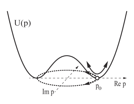
Figure 1: Schematic figure of the effective potential $U(p)=\mathcal{E}(p)-\mathcal{E}(0)$ as a function of the complex order parameter $p$, which represents the pair condensate or the pair gap.

For the sake of the discussions below, we briefly recapitulate the U(1) gauge symmetry in the Hartree-Fock-Bogoliubov (HFB) model. Consider the global U(1) gauge transformation $\left|\Psi\right\rangle\rightarrow e^{i\theta\hat{N}}\left|\Psi\right\rangle$ with $\hat{N}$ being the nucleon number operator $\hat{N}=\int d\mbox{\boldmath$r$}\sum_{\sigma}\psi^{\dagger}(\mbox{\boldmath$r$}\sigma)\psi(\mbox{\boldmath$r$}\sigma)$. The energy functional or the total Hamiltonian is symmetric with respect to the U(1) gauge transformation. However, the HFB ground state $\left|\Psi_{0}\right\rangle$ violates spontaneously this symmetry as $e^{i\theta\hat{N}}\left|\Psi_{0}\right\rangle$ differs from $\left|\Psi_{0}\right\rangle$. Correspondingly the pair condensate and the pair field are modulated in their phases as

$$\tilde{\rho}(\mbox{\boldmath$r$})\rightarrow e^{2i\theta}\tilde{\rho}(\mbox{\boldmath$r$}),\ \ \ \ \ \Delta(\mbox{\boldmath$r$})\rightarrow e^{2i\theta}\Delta(\mbox{\boldmath$r$}).$$ (7)

All the states $e^{i\theta\hat{N}}\left|\Psi_{0}\right\rangle$ transformed from one realization of the HFB ground state $\left|\Psi_{0}\right\rangle$ are also degenerate HFB ground state. This can be seen in the fact that the above equations are invariant for $\varphi_{1,i}(\mbox{\boldmath$r$}\sigma)\rightarrow e^{i\theta}\varphi_{1,i}(\mbox{\boldmath$r$}\sigma)$, $\varphi_{2,i}(\mbox{\boldmath$r$}\sigma)\rightarrow e^{-i\theta}\varphi_{2,i}(\mbox{\boldmath$r$}\sigma)$ together with Eq.(7). In the following we choose one of the HFB ground states in which the pair condensate $\tilde{\rho}(\mbox{\boldmath$r$})$ is real. In fact, the pair density and the pair potential are assumed to be real in our numerical code for the HFB ground state.

The situation is illustrated schematically in Fig.1. Here the energy gain or the effective potential $U(p)=\mathcal{E}(p)-\mathcal{E}(0)$ is shown as a function of an ”order parameter” $p$, which could be an average value of the pair condensate $\tilde{\rho}(\mbox{\boldmath$r$})$ or the pair potential $\Delta(\mbox{\boldmath$r$})$ (Details will be specified later). The order parameter $p$ is a complex variable and it transforms as $p\rightarrow e^{2i\theta}p$ under the U(1) gauge transformation. The origin $p=0$ corresponds to the Hartree-Fock ground state where the pair condensate is absent, and $p=p_{0}$ corresponds to the HFB ground state. The difference $U_{\mathrm{cond}}=\mathcal{E}(p_{0})-\mathcal{E}(0)$ is the energy gain associated with the condensation of the Cooper pairs.

Excitation modes

We describe excitation modes build on top of the HFB ground state $\left|\Psi_{0}\right\rangle$ by means of the quasi-particle random-phase approximation (QRPA). The QRPA is equivalent to describing a linear response under an external perturbation in the frame work of the time-dependent HFB theory[34, 28].

We consider a time-dependent perturbation $\mu e^{-i\omega t}\hat{V}_{\mathrm{ext}}$ where a perturbing field $\hat{V}_{\mathrm{ext}}$ belongs to a class of generalized one-body operators expressed in terms of the local density $\hat{\rho}(\mbox{\boldmath$r$})$ and the pair densities $\hat{P}(\mbox{\boldmath$r$})$ and $\hat{P}^{\dagger}(\mbox{\boldmath$r$})$:

$$\hat{V}_{\mathrm{ext}}=\int d\mbox{\boldmath$r$}\left\{v_{0}(\mbox{\boldmath$r$})\hat{\rho}(\mbox{\boldmath$r$})+v_{r}(\mbox{\boldmath$r$})\hat{P}(\mbox{\boldmath$r$})+v_{a}(\mbox{\boldmath$r$})\hat{P}^{\dagger}(\mbox{\boldmath$r$})\right\}.$$ (8)

The perturbation causes time-dependent fluctuations $\delta\rho(\mbox{\boldmath$r$},\omega)$, $\delta\tilde{\rho}(\mbox{\boldmath$r$},\omega)$ and $\delta\tilde{\rho}^{\star}(\mbox{\boldmath$r$},\omega)$ (expressed in the frequency domain) in the three densities $\rho(\mbox{\boldmath$r$})$, $\tilde{\rho}(\mbox{\boldmath$r$})$ and $\tilde{\rho}^{*}(\mbox{\boldmath$r$})$. It induces also fluctuations in the self-consistent field

$$\delta\hat{V}_{sc}(\omega)=\int d\mbox{\boldmath$r$}\left\{\delta\Gamma(\mbox{\boldmath$r$},\omega)\hat{\rho}(\mbox{\boldmath$r$})+\delta\Delta^{*}(\mbox{\boldmath$r$},\omega)\hat{P}(\mbox{\boldmath$r$})+\delta\Delta(\mbox{\boldmath$r$},\omega)\hat{P}^{\dagger}(\mbox{\boldmath$r$})\right\}$$ (9)

through the densities. Here we assume that fluctuations in the Hartree-Fock potential and the pair potential, $\delta\Gamma$ and $\delta\Delta$, are proportional to the density fluctuations $\delta\rho(\mbox{\boldmath$r$},\omega)$, $\delta\tilde{\rho}(\mbox{\boldmath$r$},\omega)$ and $\delta\tilde{\rho}^{\star}(\mbox{\boldmath$r$},\omega)$. Then the linear response of the system is governed by

$$\left(\begin{array}[]{c}\delta\rho(\mbox{\boldmath$r$},\omega)\\ \delta\tilde{\rho}(\mbox{\boldmath$r$},\omega)\\ \delta\tilde{\rho}^{\star}(\mbox{\boldmath$r$},\omega)\end{array}\right)=\int_{0}d\mbox{\boldmath$r$}^{\prime}\left(\begin{array}[]{ccc}&&\\ &R_{0}^{\alpha\beta}(\mbox{\boldmath$r$},\mbox{\boldmath$r$}^{\prime},\omega)&\\ &&\end{array}\right)\left(\begin{array}[]{l}\frac{\delta\Gamma}{\delta\rho}\delta\rho(\mbox{\boldmath$r$}^{\prime},\omega)+v_{0}(\mbox{\boldmath$r$}^{\prime})\\ \frac{\delta\Delta^{*}}{\delta\tilde{\rho}^{*}}\delta\tilde{\rho}^{\star}(\mbox{\boldmath$r$}^{\prime},\omega)+v_{r}(\mbox{\boldmath$r$}^{\prime})\\ \frac{\delta\Delta}{\delta\tilde{\rho}}\delta\tilde{\rho}(\mbox{\boldmath$r$}^{\prime},\omega)+v_{a}(\mbox{\boldmath$r$}^{\prime})\end{array}\right).$$ (10)

Here $R_{0}^{\alpha\beta}(\mbox{\boldmath$r$},\mbox{\boldmath$r$}^{\prime},\omega)$ is unperturbed density response function

$$R_{0}^{\alpha\beta}(\mbox{\boldmath$r$},\mbox{\boldmath$r$}^{\prime},\omega)=\frac{1}{2}\sum_{ij}\left\{\frac{\left\langle 0|\hat{\rho}_{\alpha}(\mbox{\boldmath$r$})|ij\right\rangle\left\langle ij|\hat{\rho}_{\beta}(\mbox{\boldmath$r$}^{\prime})|0\right\rangle}{\hbar\omega+i\epsilon-E_{i}-E_{j}}-\frac{\left\langle 0|\hat{\rho}_{\beta}(\mbox{\boldmath$r$}^{\prime})|ij\right\rangle\left\langle ij|\hat{\rho}_{\alpha}(\mbox{\boldmath$r$})|0\right\rangle}{\hbar\omega+i\epsilon+E_{i}+E_{j}}\right\}$$ (11)

with $E_{i}$ in the denominator being the excitation energy of the quasiparticle state $i$. The numerators in the r.h.s. are matrix elements of the density operators $\hat{\rho}_{\alpha}(\mbox{\boldmath$r$})=\hat{\rho}(\mbox{\boldmath$r$}),\hat{P}(\mbox{\boldmath$r$}),\hat{P}^{\dagger}(\mbox{\boldmath$r$})$ between the HFB ground state $\left|0\right\rangle=\left|\Psi_{0}\right\rangle$ and two-quasiparticle configurations $\left|ij\right\rangle=\beta_{i}^{\dagger}\beta_{j}^{\dagger}\left|\Psi_{0}\right\rangle$. Here we put the spectral representation of the unperturbed density response function expressed with discretized spectrum even for unbound quasiparticle states. The continuum nature of the unbound quasiparticle states can be taken into account explicitly using the method of the continuum QRPA formalism[34]. See Appendix for the two-quasiparticle matrix elements and the continuum QRPA.

The excited states $\left|\nu\right\rangle$ of the system appear as poles of the density fluctuations as a function of the excitation energy $\hbar\omega$. The transition matrix elements for the perturbing field is obtained through the strength function

$$S(\hbar\omega)\equiv\sum_{\nu}\left|\left\langle\nu|\hat{V}_{\mathrm{ext}}|0\right\rangle\right|^{2}\delta(\hbar\omega-E_{\nu}),$$ (12)

which can be calculated in terms of the solution of the linear response equation:

$$S(\hbar\omega) =-\frac{1}{\pi}\mathrm{Im}\langle\hat{V}_{\mathrm{ext}}^{\dagger}\rangle(\omega)$$

$$=-\frac{1}{\pi}\mathrm{Im}\int d\mbox{\boldmath$r$}\left\{v_{0}^{*}(\mbox{\boldmath$r$})\delta\rho(\mbox{\boldmath$r$},\omega)+v_{a}^{*}(\mbox{\boldmath$r$})\delta\tilde{\rho}(\mbox{\boldmath$r$},\omega)+v_{r}^{*}(\mbox{\boldmath$r$})\delta\tilde{\rho}^{\star}(\mbox{\boldmath$r$},\omega)\right\}.$$ (13)

Model parameters and numerical details

We discuss the pairing correlation of neutrons in semi-magic Sn isotopes, for which the ground states are expected to be spherical. We adopt the SLy4 parameter set[35] for the Skyrme energy functional. The pairing interaction defining the pairing energy functional is the density dependent delta interaction (DDDI), the contact force whose interaction strength depends on the position through the nucleon density:

$$v^{{\rm pair}}_{q}(\mbox{\boldmath$r$},\mbox{\boldmath$r$}^{\prime}) ={1\over 2}(1-P_{\sigma})V_{q}(\mbox{\boldmath$r$})\delta(\mbox{\boldmath$r$}-\mbox{\boldmath$r$}^{\prime}),\ \ \ (q=n,p)$$ (14)

$$V_{q}(\mbox{\boldmath$r$}) =v_{0}\left(1-\eta\left({\rho_{q}(\mbox{\boldmath$r$})\over\rho_{0}}\right)^{\alpha}\right).$$ (15)

Correspondingly the pair potential is given by $\Delta_{q}(\mbox{\boldmath$r$})=V_{q}(\mbox{\boldmath$r$})\tilde{\rho}_{q}(\mbox{\boldmath$r$}).$ In the actual calculation, we assume the spherical HFB mean-field and solve all the equations using the polar coordinate system and the partial wave expansion. The radial coordinate is truncated at $r=R_{\mathrm{max}}$ with $R_{\mathrm{max}}=20$fm. The partial waves are taken into account up to the maximum angular quantum number $l_{\mathrm{max}},j_{\mathrm{max}}=12,25/2$. We truncate the quasiparticle states by maximum quasiparticle energy $E_{\mathrm{max}}=60$ MeV. The radial coordinate is discretized with an interval $\Delta r=0.2$fm. The parameters of the DDDI are $v_{0}=-458.4$ MeV fm^-3, $\rho_{0}=0.08$ fm^-3, $\alpha=0.845$, and $\eta=0.71$ which are chosen to reproduce the scattering length of the nuclear force in the ${}^{1}S_{0}$ channel and the experimental gap in ¹²⁰Sn[31]. The HFB equation is solved with the Runge-Kutta method with box boundary condition, i.e $\phi(r)=0$ at $r=R$. With this boundary condition, unbound quasiparticle states have discrete spectrum, and the resultant strength function does also. It is possible to impose the proper boundary condition appropriate for unbound and continuum quasiparticle states using the framework of the continuum QRPA[34, 30, 31, 32, 33] (See also Appedix). The QRPA calculation is performed using the discretized spectral representation while the continuum QRPA is also used in some examples. The smoothing parameter is $\epsilon=100$ keV.

III Pair vibrations and Higgs response

III.1 Response to pair transfer operators

Figure 2: Pair-addition and pair-removal strength functions, $S_{\mathrm{ad}}(E)$ and $S_{\mathrm{rm}}(E)$, for neutrons in ¹²⁰Sn, plotted as functions of the excitation energy $E$. The unit of the strength functions is MeV^-1 since $\hat{P}_{\mathrm{ad}}$ and $\hat{P}_{\mathrm{rm}}$ are dimensionless. The solid line is the result of the QRPA calculation based on the discretized spectral representation of the response function while the dotted line is the result of the continuum QRPA. The smoothing width is $\epsilon=100$ keV.

Figure 3: Pair-addition and pair-removal transition densities $r^{2}P^{(\mathrm{ad})}_{\nu}(r)$ (solid curve) and $r^{2}P^{(\mathrm{rm})}_{\nu}(r)$ (dotted curve) of neutrons for some peaks seen in the pair-addition and pair-removal strength functions for ¹²⁰Sn, shown in Fig.2.

Sensitive probes to the pairing correlation may be expressed in terms of the pair field operators $\hat{P}(\mbox{\boldmath$r$})=\psi(\mbox{\boldmath$r$}\uparrow)\psi(\mbox{\boldmath$r$}\downarrow)$ and $\hat{P}^{\dagger}(\mbox{\boldmath$r$})=\psi^{\dagger}(\mbox{\boldmath$r$}\downarrow)\psi^{\dagger}(\mbox{\boldmath$r$}\uparrow)$. We define a pair-addition operator

$$\hat{P}_{\mathrm{ad}}=\int d\mbox{\boldmath$r$}Y_{00}f(r)\hat{P}^{\dagger}(\mbox{\boldmath$r$})=\frac{1}{\sqrt{4\pi}}\int d\mbox{\boldmath$r$}f(r)\psi^{\dagger}(\mbox{\boldmath$r$}\downarrow)\psi^{\dagger}(\mbox{\boldmath$r$}\uparrow)$$ (16)

and a pair-removal operator

$$\hat{P}_{\mathrm{rm}}=\int d\mbox{\boldmath$r$}Y_{00}f(r)\hat{P}(\mbox{\boldmath$r$})=\frac{1}{\sqrt{4\pi}}\int d\mbox{\boldmath$r$}f(r)\psi(\mbox{\boldmath$r$}\uparrow)\psi(\mbox{\boldmath$r$}\downarrow).$$ (17)

These operators bring about a transition changing particle number by $\Delta N=\pm 2$. Here we introduce a form factor $f(r)$ which is effective in a spatial region where the nucleon density is finite, but diminishes far outside the nucleus as we are interested in a process where a nucleon pair is added to or removed from a nucleus. Specifically we choose a Woods-Saxon function,

$$f(r)=\frac{1}{1+\exp((r-R)/a)}$$ (18)

with $R=1.27\times A^{1/3}$ fm and $a=0.67$ fm, but as shown later the main conclusion does not depend on detailed form of $f(r)$. In the present study we describe the pair vibration with the lowest multipolarity $J^{\pi}=0^{+}$. Here $Y_{00}$ is the spherical harmonics with rank 0 and both $\hat{P}_{\mathrm{ad}}$ and $\hat{P}_{\mathrm{rm}}$ carry the angular and parity quantum numbers $0^{+}$. We describe the pair vibration with spin parity $J^{\pi}=0^{+}$.

Response of a nucleus against these operators are represented by the strength functions

$$S_{\mathrm{ad}}(E)=\sum_{\nu}\left|\left\langle\nu|\hat{P}_{\mathrm{ad}}|0\right\rangle\right|^{2}\delta(E-E_{\nu})$$ (19)

for the pair-addition process, and

$$S_{\mathrm{rm}}(E)=\sum_{\nu}\left|\left\langle\nu|\hat{P}_{\mathrm{rm}}|0\right\rangle\right|^{2}\delta(E-E_{\nu})$$ (20)

for the pair-removal process. Here $\left|\nu\right\rangle$ is the QRPA excited states with excitation energy $E_{\nu}$ whereas $\left\langle\nu|\hat{P}_{\mathrm{ad}}|0\right\rangle$ and $\left\langle\nu|\hat{P}_{\mathrm{rm}}|0\right\rangle$ is the matrix elements of the pair-add and pair-removal operators between the HFB ground state $\left|0\right\rangle=\left|\Psi_{0}\right\rangle$ and the QRPA excited states. Transition densities

$$P^{(\mathrm{ad})}_{\nu}(\mbox{\boldmath$r$}) =\left\langle\nu|\hat{P}^{\dagger}(\mbox{\boldmath$r$})|0\right\rangle=\left\langle\nu|\psi^{\dagger}(\mbox{\boldmath$r$}\downarrow)\psi^{\dagger}(\mbox{\boldmath$r$}\uparrow)|0\right\rangle=P^{(\mathrm{ad})}_{\nu}(r)Y_{00}^{*},$$ (21)

$$P^{(\mathrm{rm})}_{\nu}(\mbox{\boldmath$r$}) =\left\langle\nu|\hat{P}(\mbox{\boldmath$r$})|0\right\rangle=\left\langle\nu|\psi(\mbox{\boldmath$r$}\uparrow)\psi(\mbox{\boldmath$r$}\downarrow)|0\right\rangle=P^{(\mathrm{rm})}_{\nu}(r)Y_{00}^{*},$$ (22)

representing amplitudes of pair-addition and -removal are also useful measures to look into structure of the excited states.

Figure 2 (a) and (b) show the pair-add and pair-removal strength functions, respectively, calculated for neutrons in ¹²⁰Sn. The results exhibit several noticeable peaks. We first discuss them referring to the concept of the pair rotation and the pair vibration.

First, we note the peak with the lowest excitation energy $E=0.60$ MeV, which is seen both in the pair-addition and in the pair-removal strength functions. It corresponds to the pair rotation, i.e. the transition from the ground state of the system $N$ to the ground state with $N\pm 2$. The pair rotation, which is associated with a displacement along the dashed line in Fig.1, should appear as a zero-energy Nambu-Goldstone mode arising from the the gauge transformation $e^{i\theta\hat{N}}\left|\Psi_{0}\right\rangle$. In the actual numerical implementation of the HFB+QRPA formalism, the calculated excitation energy of the pair rotation deviates from zero by a small amount, 0.60 MeV in the present case, due to numerical errors and truncations. The transition densities of the lowest energy peak, the pair rotation mode, are shown in Fig.3. It is seen that the pair-addition transition density and the pair-removal one has the same shape as functions of $r$, but they have the opposite phases. This is what is expected for the pair rotation, since the phase change in the pair condensate $\tilde{\rho}(\mbox{\boldmath$r$})$ gives $\delta\tilde{\rho}(\mbox{\boldmath$r$})=\delta e^{2i\delta\theta}\tilde{\rho}(\mbox{\boldmath$r$})\sim 2i\delta\theta\tilde{\rho}(\mbox{\boldmath$r$})$ and $\delta\tilde{\rho}^{*}(\mbox{\boldmath$r$})=\delta e^{-2i\delta\theta}\tilde{\rho}(\mbox{\boldmath$r$})\sim-2i\delta\theta\tilde{\rho}(\mbox{\boldmath$r$})$, i.e., opposite sign in these quantities with a common shape proportional to the ground state pair condensate $\tilde{\rho}(\mbox{\boldmath$r$})$.

Other peaks in Fig.2(a) and (b) represent transitions to excited $0^{+}$ states in the neighbor nuclei. The peak at $E=2.44$ MeV, the lowest excited $0_{2}^{+}$ state, has transition strengths which are not very large. This state corresponds to the pair vibration, which is predicted to be a lowest excited $0_{2}^{+}$ state with energy about $2\Delta$[20, 21, 1]. The excitation energy 2.44 MeV is consistent with the predicted value $E\approx 2\Delta$ as an average value of the pair gap is $\Delta=\int d\mbox{\boldmath$r$}\rho(r)\Delta(r)/\int d\mbox{\boldmath$r$}\rho(r)=1.15$ MeV in the present case.

In the interval of excitation energy from 3 MeV up to around 20 MeV, there exist several peaks which have larger pair-addition or -removal strengths than those of the pair vibration at $E=2.44$ MeV, e.g. peaks at $E=12.36$ and 17.45 MeV seen in the pair-addition strength, and those at $E=3.85$ and 17.31 MeV in the pair-removal strength. These states may also be regarded as pair vibrational states as the pair-transfer strengths are enhanced by the RPA correlation (see below). Although high-lying pair vibration is often called the giant pair vibration (GPV)[24, 27, 25, 26], we adopt in the present paper a more inclusive term ”high-lying pair vibrations” for these peaks since the strength distribution does not form a single giant peak, but rather multiple peaks in a wide energy interval.

We remark that the low-lying pair vibration at $E=2.44$ MeV and other high-lying pair vibrations have slightly different characters. The low-lying pair vibration has both the pair-addition and -removal strengths whereas the high-lying pair vibrations have either the pair-addition strength or the pair-removal strengths. This difference is also clearly seen in the transition density, shown in Fig.3: the low-lying pair vibration at $E=2.44$ MeV has both the pair-addition and pair-removal amplitudes. Contrastingly the high-lying pair vibrations are seen either in the pair-addition strength function or in the pair-removal strength function, but not in the both. This is reflected also in the transition density. As shown in Fig.3, the transition density of the peaks at $E=12.31$ MeV and $E\approx 17.45$ MeV seen in the pair-addition strength function have large pair-addition amplitude while the pair-removal amplitude is almost negligible. These states can be populated only by the pair-addition process. On the contrary, the peaks at $E=3.85$ and 17.31 MeV existing in the pair-removal strength function have dominant amplitude for the pair-removal transition density.

III.2 Higgs response

Figure 4: (a) Higgs strength function $S_{\mathrm{H}}(E)$ of neutrons for ¹²⁰Sn, plotted as functions of the excitation energy $E$. (b) Sum of the pair-addition and pair-removal strength functions, $S_{\mathrm{ad}}(E)+S_{\mathrm{rm}}(E)$. (c) Unperturbed Higgs strength function $S_{\mathrm{H}}(E)$ for uncorrelated neutron two-quasiparticle excitations.

We shall here address a question how the pair vibrations discussed above are related to the macroscopic picture as an amplitude oscillation of the order parameter, the Higgs mode. However, the existence of multiple states, including both the low-lying and high-lying pair vibrations, makes it difficult to relate this macroscopic picture to one of the pair vibrational states. We need a new way of characterizing the pair vibrations, which is more suitable for obtaining the macroscopic information.

As is illustrated by Fig.1, response of the pair fields around a HFB equilibrium point has two different directions with respect to the order parameter of the pair condensation: the phase mode changing the phase of the pair gap (or the pair condensate), and the other changing the amplitude of the pair gap/condensate. The pair-add operators, $\hat{P}_{\mathrm{ad}}\sim\psi^{\dagger}\psi^{\dagger}$, and the pair-removal operators $\hat{P}_{\mathrm{rm}}\sim\psi\psi$, do not probe separately these two different modes since both the pair rotation (the phase mode) and the pair vibrations (possible amplitude mode) are seen in both of the pair-addition and pair-removal strengths functions.

Instead we introduce a pair field operator that is a linear combination of $\hat{P}_{\mathrm{ad}}$ and $\hat{P}_{\mathrm{rm}}$:

$$\hat{P}_{\mathrm{H}}=\hat{P}_{\mathrm{ad}}+\hat{P}_{\mathrm{rm}}=\frac{1}{\sqrt{4\pi}}\int d\mbox{\boldmath$r$}f(r)\left\{\psi(\mbox{\boldmath$r$}\uparrow)\psi(\mbox{\boldmath$r$}\downarrow)+\psi^{\dagger}(\mbox{\boldmath$r$}\downarrow)\psi^{\dagger}(\mbox{\boldmath$r$}\uparrow)\right\}.$$ (23)

Note that fluctuation of the amplitude $|\tilde{\rho}(\mbox{\boldmath$r$})|$ of the pair condensate reads $\delta|\tilde{\rho}(\mbox{\boldmath$r$})|=\left(\tilde{\rho}(\mbox{\boldmath$r$})\delta\tilde{\rho}^{*}(\mbox{\boldmath$r$},t)+\tilde{\rho}^{*}(\mbox{\boldmath$r$})\delta\tilde{\rho}(\mbox{\boldmath$r$},t)\right)/2|\tilde{\rho}(\mbox{\boldmath$r$})|=(\delta\tilde{\rho}^{*}(\mbox{\boldmath$r$},t)+\delta\tilde{\rho}(\mbox{\boldmath$r$},t))/2$ for real $\tilde{\rho}(\mbox{\boldmath$r$})$, and therefore the Higgs operator $\hat{P}_{\mathrm{H}}$ defined by Eq.(23) probes the amplitude fluctuation. In the following, we call $\hat{P}_{\mathrm{H}}$ the Higgs operator after the nomenclature that the amplitude mode of the pair field is often called Higgs mode[15, 16]. The strength function for the Higgs operator is defined by

$$S_{\mathrm{H}}(E)=\sum_{\nu}\left|\left\langle\nu|\hat{P}_{\mathrm{H}}|0\right\rangle\right|^{2}\delta(E-E_{\nu}).$$ (24)

Figure 4 (a) is the calculated Higgs strength function $S_{\mathrm{H}}(E)$ of neutrons for ¹²⁰Sn. For comparison we show in Fig.4(b) a sum $S_{\mathrm{ad}}(E)+S_{\mathrm{rm}}(E)$ of the pair-addition and pair-removal strength functions (Fig.2). The panel (c) is a Higgs strength function for independent two-quasiparticle excitations, namely a calculation in which the RPA correlation is removed. We observe the following features.

We first note that, compared with the uncorrelated result (c), the Higgs strength in (a) is enhanced by several times for the peaks of low-lying and high-lying pair vibrations. This clearly indicates collectivity of both the low- and high-lying pair vibrations.

Secondly we observe that the Higgs strength function is close to the sum of the pair-addition and pair-removal strengths although there are some differences. A significant and important difference is seen for the pair rotation mode (the peak at $E=0.60$ MeV in this example), for which the Higgs strength almost invisible. Indeed, it should vanish in principle due to the very nature of the phase mode associated with the U(1) gauge symmetry. As discussed above, the pair-add and pair-removal amplitudes of the phase mode have the same shape but with opposite sign (cf. Fig.3), and consequently these two amplitudes cancel each other in the matrix element of the Higgs operator $\left\langle\nu|\hat{P}_{\mathrm{H}}|0\right\rangle=\left\langle\nu|\hat{P}_{\mathrm{ad}}|0\right\rangle+\left\langle\nu|\hat{P}_{\mathrm{rm}}|0\right\rangle=0$.

For the low-lying pair vibration (the peak at $E=2.44$ MeV), contrastingly, the Higgs strength is enhanced. Namely it is more than the sum of the pair-addition and pair-removal strengths (It is approximately two times the sum). This is because the both pair-addition and pair-removal transition densities of this mode have the same sign, as seen in Fig.3, and they leads to a coherent sum in the matrix element of the Higgs operator $\left\langle\nu|\hat{P}_{\mathrm{H}}|0\right\rangle=\left\langle\nu|\hat{P}_{\mathrm{ad}}|0\right\rangle+\left\langle\nu|\hat{P}_{\mathrm{rm}}|0\right\rangle$. Consequently the low-lying pair vibration contributes more strongly to the Higgs strength than to the pair-addition and pair-removal strengths. Because of this enhancement due to the coherence, the low-lying pair vibration could be regarded as an Higgs mode in nuclei. This interpretation might be supported also by the energy relation $E\approx 2\Delta$ of the low-lying pair vibration, which is also the case for the Higgs mode in the superconductors[10, 14, 15, 16] with the energy relation $E=2\Delta$. However, for the reasons below we reserve possible identification of the low-lying pair vibration as the Higgs mode.

The high-lying pair vibrations, emerging as several peaks distributed up to around $E\sim 20$ MeV, have the Higgs strength comparable to that of the low-lying pair vibration. From the viewpoint of the response to the Higgs operator, the high-lying pair vibrations may also be candidates of the Higgs mode. However the energy relation $E=2\Delta$ does not hold. The high-lying pair vibrations exhibit no coherence between the matrix elements $\left\langle\nu|\hat{P}_{\mathrm{ad}}|0\right\rangle$ and $\left\langle\nu|\hat{P}_{\mathrm{rm}}|0\right\rangle$. The Higgs strengths of these states are incoherent sum of the pair-addition and -removal strengths. It may not be reasonable to identify either the high-lying or the low-lying pair vibrations as a pure Higgs mode.

III.3 Static polarizability

The Higgs strength is not concentrated to a single state, but distributed over many excited states, including both the low-lying and high-lying pair vibrations. Since there seems no one single pair vibrational state interpreted as a pure Higgs mode, we need a different viewpoint which integrates both the low- and high-lying pair vibrations. Here we consider the static polarizability which can be derived from the Higgs strength function. It is defined by

$$\alpha_{\mathrm{H}}=\frac{d\langle\hat{P}_{\mathrm{H}}\rangle^{\prime}}{d\mu},$$ (25)

where $\langle\hat{P}_{\mathrm{H}}\rangle^{\prime}$ is a change of the expectation value under the static perturbation $\hat{V}_{\mathrm{ext}}=\mu\hat{P}_{\mathrm{H}}$. The static polarizability is related to the strength function through the inversely energy weighted sum

$$I_{-1}=2\int_{E_{\mathrm{min}}}^{E_{\mathrm{max}}}dE\frac{S_{\mathrm{H}}(E)}{E}=2\sum_{\nu}\frac{\left|\left\langle\nu|\hat{P}_{\mathrm{H}}|0\right\rangle\right|^{2}}{E_{\nu}}=\alpha_{\mathrm{H}}$$ (26)

of the Higgs strength function $S_{\mathrm{H}}(E)$. In other words, the static polarizability for the Higgs operator, called Higgs polarizablility hereafter, can be evaluated if the Higgs strength function is obtained. We note that the inversely energy-weighted sum and the static polarizability has been discussed intensively for the case of the E1 strength function, i.e. the electric dipole excitations in nuclei, as a probe of neutron skin and nuclear matter properties [36, 37, 38, 39, 40].

In the present study the inversely weighted sum is calculated by taking an integral in an energy interval from $E_{\mathrm{min}}=1.1$ MeV to the upper limit of the excitation energy $E_{\mathrm{max}}=60$ MeV. The lower bound is set to exclude the contribution from the pair rotation, which should have vanished if the complete selfconsistency is fulfilled in the numerical calculation. Figure 5 is a running sum of Eq.(26) where the upper bound $E_{\mathrm{max}}$ is varied. It is seen that although the contribution of the low-lying pair vibration mode (the lowest excitation) is as large as about 35% of the total sum, strengths distributed at higher excitation energies contribute significantly. The large strengths of the high-lying pairing vibrations (distributed up to around 20 MeV), gives sizable contribution of about 45% (i.e. 80% including all up to 20 MeV) to the total sum. Contributions of strengths above 20 MeV is small, and there is no distinct distribution of the strengths.

Figure 5: Inversely energy-weighted sum $I_{-1}(E_{\mathrm{max}})$ of the Higgs strength function for ¹²⁰Sn, as a function of the maximum excitation energy $E_{\mathrm{max}}$ of the sum.

IV Pair condensation energy

IV.1 Effective potential

Figure 6: The potential energy curve as a function of the order parameter $p=\langle\hat{P}_{\mathrm{H}}\rangle$ for ¹²⁰Sn, ¹³²Sn and ¹⁴⁰Sn. The total energy obtained with the constrained Hartree-Fock-Bogoliubov (CHFB) calculation is plotted with the diamond symbol. The dashed curve is a quartic function, Eq.(29), fitted to the CHFB results.

Let us now relate the above results to the macroscopic picture discussed with Fig.1. For this purpose we specify the order parameter and the effective potential.

As the order parameter we adopt the expectation value of the pair removal operator

$$p=2\langle\hat{P}_{\mathrm{rm}}\rangle=\frac{1}{\sqrt{\pi}}\int d\mbox{\boldmath$r$}f(r)\tilde{\rho}(\mbox{\boldmath$r$}),$$ (27)

which also represents a spatial integral (or average) of the pair condensate $\tilde{\rho}(\mbox{\boldmath$r$})$. (The factor of two is put here just for later convenience). The order parameter $p$ is a complex variable as it follows $p\rightarrow e^{2i\theta}p$ under the U(1) gauge transformation. We then consider the total energy of the system $\mathcal{E}(p)$ as the effective potential, a function of the order parameter $p$. Because of the U(1) symmetry $\mathcal{E}(p)$ depends only on the amplitude $|p|$, and it is sufficient to consider the potential curve along the real axis of $p$, which corresponds to the expectation value of the Higgs operator $\hat{P}_{\mathrm{H}}$. In the following analysis we use

$$p=\langle\hat{P}_{\mathrm{H}}\rangle$$ (28)

which in fact represents the amplitude $|p|$ of the order parameter.

The effective potential $U(p)=\mathcal{E}(p)-\mathcal{E}(0)$ can be calculated with the total energy $\mathcal{E}(p)$ for the generalized Slater determinant $\left|\Psi(p)\right\rangle$, which is obtained by means of the constrained Hartree-Fock-Bogoliubov (CHFB) calculation[5] using $\hat{P}_{\mathrm{H}}$ as a constraining operator.

Figure 6 shows the effective potential calculated for ¹²⁰Sn, ¹³²Sn and ¹⁴⁰Sn. Let us focus on the representative example of ¹²⁰Sn. The effective potential in this example has a so-called Mexican hat shape, which has a minimum at finite $p=p_{0}$ where $p_{0}=\langle\hat{P}_{\mathrm{H}}\rangle$ corresponds to the HFB ground state $\left|\Psi_{0}\right\rangle$. Since the shape is smooth as a function of $p$, it may be approximated by a polynomial. Guided by the Ginzburg-Landau theory of the superconductivity[9], we here assume a fourth-order polynomial

$$U_{\mathrm{4th}}(p)=ap^{4}+bp^{2}+c,$$ (29)

and we fit this function to the calculated effective potential $\mathcal{E}(p)$. As seen in Fig.6, the fourth-order polynomial is a good representation of the CHFB results. We have checked and confirmed good accuracy of Eq.(29) for other even-even Sn isotopes, see two other examples in Fig.6.

IV.2 Pair condensation energy

In the case where the effective potential is approximated well by the fourth-order polynomial there holds a simple relation between the potential parameters, $a$ and $b$, and the order parameter $p_{0}$ and the curvature $C$ of the effective potential at the potential minimum:

$$p_{0} =\sqrt{\frac{-b}{2a}},$$ (30)

$$C =\left.\frac{d^{2}U_{\mathrm{4th}}(p)}{d^{2}p}\right|_{p=p_{0}}=-4b.$$ (31)

As a consequence, the potential depth $D$ can be also related to the two parameters characterizing the minimum:

$$D=U_{\mathrm{4th}}(p_{0})-U_{\mathrm{4th}}(0)=-\frac{b^{2}}{4a}=-\frac{1}{8}Cp_{0}^{2}.$$ (32)

We remark here that the parameters $p_{0}$ and $C$ can be derived from the Higgs response. The order parameter $p_{0}$ at the minimum is the expectation value of the Higgs operator for the ground state

$$p_{0}=\left\langle\Psi_{0}|\hat{P}_{\mathrm{H}}|\Psi_{0}\right\rangle.$$ (33)

The potential curvature $C$ at the minimum $p=p_{0}$ is related to the Higgs polarizability $\alpha_{\mathrm{H}}$, Eq.(25),

$$C=1/\alpha_{\mathrm{H}}$$ (34)

through the Hellmann-Feynman theorem[41, 5]. Consequently the potential depth $D$, which can be interpreted as the pair condensation energy $U_{\mathrm{cond}}=\mathcal{E}(p_{0})-\mathcal{E}(0)$, can be evaluated as

$$U_{\mathrm{cond}}^{\mathrm{Higgs}}=-\frac{1}{8}\frac{p_{0}^{2}}{\alpha_{\mathrm{H}}}$$ (35)

using the Higgs polarizability $\alpha_{\mathrm{H}}$. Note that the quantities in the last expression can be evaluated using the matrix element of the Higgs operator $\hat{P}_{\mathrm{H}}$ for the ground state $\left|\Psi_{0}\right\rangle$, and the strength function of the Higgs operator $\hat{P}_{\mathrm{H}}$, i.e. the information of the Higgs response of the system.

The pair condensation energy in ¹²⁰Sn obtained using the Higgs response, i.e. Eq.(35). is $U_{\mathrm{cond}}^{\mathrm{Higgs}}=1.51$ MeV. It is compared the pair condensation energy obtained directly from the CHFB calculation, $U_{\mathrm{cond}}^{\mathrm{CHFB}}=1.58$ MeV. It is found that the evaluation using the Higgs response reproduces the actual value ( obtained directly from the CHFB calculation) within an error less than 10 %. It suggests that the pair condensation energy may be evaluated via the Higgs response with good accuracy.

V Sn isotopes

Figure 7: (a)The order parameter $p_{0}=\langle\hat{P}_{\mathrm{H}}\rangle$ and the average pair gap $\Delta$ of neutrons, calculated for the ground states of the Sn isotopes. (b) The static polarizability $\alpha_{\mathrm{H}}$ for the Higgs operator $\hat{P}_{H}$, calculated from the inversely energy weighted sum of the Higgs strength function.

Figure 8: The pair condensation energy $U_{\mathrm{cond}}^{\mathrm{Higgs}}$ evaluated using the Higgs strength function in the Sn isotopes is plotted with crosses. It is compared with the pair condensation energy $U_{\mathrm{cond}}^{\mathrm{CHFB}}$ which is calculated directly using the constrained Hartree-Fock-Bogoliubov method, plotted with circles. The dotted line is an analytic estimate $\frac{1}{2}g\Delta^{2}$ with the oscillator estimate of the single-particle level density $g=0.015A$ MeV^-1.

We shall apply the above method of evaluating the pair condensation energy to the neutron pair correlation in even-even Sn isotopes covering from doubly-magic neutron-deficient ¹⁰⁰Sn to neutron-rich ¹⁵⁰Sn. The ground state value of the order parameter $p_{0}=\langle\hat{P}_{\mathrm{H}}\rangle$ as well as the average pairing gap $\Delta=\int d\mbox{\boldmath$r$}\rho(r)\Delta(r)/\int d\mbox{\boldmath$r$}\rho(r)$ are shown in Fig.7 (a). It is seen that these two quantities are essentially proportional to each others. They are zero in neutron magic nuclei ¹⁰⁰Sn and ¹³²Sn, where the pair condensate vanishes due to a large shell gap at the neutron Fermi energy, corresponding to the ”normal” phase.

Figure 7 (b) shows the Higgs polarizability $\alpha_{\mathrm{H}}$, evaluated from the Higgs strength function. A noticeable feature is that its neutron number dependence is not correlated with that of the pairing gap $\Delta$ or the order parameter $p_{0}=\langle\hat{P}_{\mathrm{H}}\rangle$. For instance the Higgs polarizability in the closed-shell nuclei ¹⁰⁰Sn and ¹³²Sn is larger than neighboring isotopes. It is also remarkable that the largest value is in ¹⁴⁰Sn where the pairing gap takes an intermediate value.

Figure 8 is the pair condensation energy $U_{\mathrm{cond}}^{\mathrm{Higgs}}$ of neutrons evaluated from the Higgs response, i.e. using Eq.(35). It is compared with the pair condensation energy $U_{\mathrm{cond}}^{\mathrm{CHFB}}$ which is calculated directly using the constrained Hartree-Fock-Bogoliubov method for several isotopes. We confirm that the proposed method works well not only for ¹²⁰Sn discussed above, but also for the other isotopes.

Another point is that the isotopic trend of the pair condensation energy shows some resemblance and difference from that of the pair gap. For comparison we plot also an estimate of the pair condensation energy $\frac{1}{2}g\Delta^{2}$ based on the equidistant single-particle model[5] where $g$ is the single-particle level density. This estimate reflects the pair correlation through the pair gap alone. It is seen that the microscopic condensation energy differs from this estimate with respect to both the magnitude and the isotopic dependence. This points to that the pair condensation energy is a physical quantity which carries information not necessarily expected from the pairing gap.

A noticeable example is ¹⁴⁰Sn, where the pair condensation energy is very small (about 0.1 MeV). The small condensation energy is due to the large value of the Higgs polarizability (see Fig.7 (c) ), and its origin is seen in the Higgs strength function, shown in Fig.9. The small pair condensation energy, reflecting the very shallow effective potential with small potential curvature (Fig.6(a)), manifests itself as the presence of the low-lying pair vibration which has a very large Higgs strength, several times larger than that in ¹²⁰Sn.

We also note ¹³²Sn, in which the HFB ground state has no pair condensate. Correspondingly the effective potential shown in Fig. 6 (b) has the minimum at $p_{0}=0$, and there is no pair rotation in this case. The Higgs polarizability (or the potential curvature at the minimum) in this case is slightly larger (smaller) than that for ¹²⁰Sn (see Fig.7 (b) and Fig.6 ). This feature can be traced to the presence of the pair vibrations with relatively large pair-transfer strengths as seen in Fig.9.

Figure 9: Higgs strength function $S_{\mathrm{H}}(E)$ for ¹²⁰Sn, ¹³²Sn and ¹⁴⁰Sn, calculated with the continuum QRPA.

VI Discussion

The method to evaluate the pair condensation energy from the Higgs response should not depend on details of the definitions of the pair transfer operators $\hat{P}_{\mathrm{ad}}$, $\hat{P}_{\mathrm{rm}}$ and $\hat{P}_{\mathrm{H}}$. We have checked other choices of the form factor $f(r)$ appearing in Eqs.(16) and (17) by using $f(r)=\frac{d}{dr}\frac{1}{1+\exp((r-R)/a)}$ and $f(r)=\frac{r^{2}}{1+\exp((r-R)/a)}$, both of which have a weight on the surface area of the nucleus. The pair condensation energy derived from the Higgs response in ¹²⁰Sn is $U^{\mathrm{Higgs}}_{\mathrm{cond}}=1.51$ MeV and $1.58$ MeV for the above two choices. They coincide well with $U^{\mathrm{Higgs}}_{\mathrm{cond}}=1.51$ MeV obtained with the volume-type form factor $f(r)=\frac{1}{1+\exp((r-R)/a)}$. We also note that Eq. (35) for the pair condensation energy is expressed with a relative quantity $\alpha_{\mathrm{H}}/p_{0}^{2}$, for which relevant are not the absolute value but relative transition strengths $S_{\mathrm{H}}(E)/p_{0}^{2}$ or $\left\langle\nu|\hat{P}_{\mathrm{H}}|0\right\rangle^{2}/\langle\hat{P}_{\mathrm{H}}\rangle^{2}$ normalized by the ground state matrix element $p_{0}=\langle\hat{P}_{\mathrm{H}}\rangle$.

We envisage application of the present method to experimental studies using two-neutron transfer reactions, such as $(p,t)$ and $(t,p)$ reactions. As discussed in Ref.[19, 21, 1], the cross sections of a two-neutron stripping and pick-up reactions may be related to matrix elements of the pair-addition and the pair-removal operators if one assumes a one-step process. In this simple picture, the transition amplitude for the ground-to-ground transition $N\rightarrow N\pm 2$ may correspond to matrix elements $\left\langle 0_{\mathrm{gs}}^{+},N+2|\hat{P}_{\mathrm{ad}}|0_{\mathrm{gs}}^{+},N\right\rangle$ and $\left\langle 0_{\mathrm{gs}}^{+},N-2|\hat{P}_{\mathrm{rm}}|0_{\mathrm{gs}}^{+},N\right\rangle$, which is approximated by the expectation value $\left\langle\Psi_{0}|\hat{P}_{\mathrm{ad}}|\Psi_{0}\right\rangle=\left\langle\Psi_{0}|\hat{P}_{\mathrm{rm}}|\Psi_{0}\right\rangle=\langle\hat{P}_{\mathrm{H}}\rangle/2$ for the HFB ground state $\left|\Psi_{0}\right\rangle$. Thus the ground-to-ground pair transfer is expected to provide the order parameter $p_{0}=\langle\hat{P}_{\mathrm{H}}\rangle$. Similarly the two-neutron transfer cross sections populating excited $0^{+}$ states may be related to matrix elements $\left\langle 0_{\nu}^{+},N+2|\hat{P}_{\mathrm{ad}}|0_{\mathrm{gs}}^{+},N\right\rangle$ and $\left\langle 0_{\nu}^{+},N-2|\hat{P}_{\mathrm{rm}}|0_{\mathrm{gs}}^{+},N\right\rangle$, which correspond to the matrix elements $\left\langle\nu|\hat{P}_{\mathrm{ad}}|0\right\rangle$ and $\left\langle\nu|\hat{P}_{\mathrm{rm}}|0\right\rangle$ for the QRPA excited states $\left|\nu\right\rangle$. We thus expect that two-neutron stripping and pick-up reactions populating excited $0^{+}$ states provides the pair-addition and pair-removal strength functions, $S_{\mathrm{ad}}(E)$ and $S_{\mathrm{rm}}(E)$. The Higgs strength function $S_{\mathrm{H}}(E)$ is then evaluated as a sum of $S_{\mathrm{ad}}(E)$ and $S_{\mathrm{rm}}(E)$ (cf. Fig.4). Here transition to the low-lying pair vibration needs to be treated separately since for this case the Higgs transition amplitude is a coherent sum of the amplitudes $\left\langle\nu|\hat{P}_{\mathrm{ad}}|0\right\rangle$ and $\left\langle\nu|\hat{P}_{\mathrm{rm}}|0\right\rangle$. Once the Higgs strength function is obtained in this way, the Higgs polarizability $\alpha_{\mathrm{H}}$ can be evaluated. Consequently, combining $p_{0}$ and $\alpha_{\mathrm{H}}$ thus obtained, we may estimate the neutron pair condensation energy $U_{\mathrm{cond}}^{\mathrm{Higgs}}$ using Eq.(35). Note that this argument based on the one-step picture may be simplistic from a viewpoint of the reaction mechanisms, such as the finite range effect and the two-step processes[23]. More quantitative analysis of the two-nucleon transfer reactions needs to be explored in detail. However it is beyond the scope of the present work, and we leave it for a future study.

VII Conclusions

We have discussed a new idea of the Higgs response, which probes the Cooper pair condensate in pair correlated nuclei. It is based on the analogy between the pair correlated nuclei and the superfluid/superconducting state in infinite Fermi systems. The latter systems exhibit characteristic collective excitation modes which emerge as a consequence of the spontaneous violation of the U(1) gauge symmetry; the Higgs mode, the amplitude oscillation of the pair condensate, and the Nambu-Goldstone mode (or the Anderson-Bogoliubov mode in neutral superfluid systems), the phase oscillation of the pair condensate. In the present study, we explored possible counterpart of the Higgs mode in finite nuclei.

For this purpose, we considered a new kind of pair-transfer operator, the Higgs operator, which probes the amplitude motion of the pair condensate. We then described the strength function for the Higgs operator by means of the quasiparticle random phase approximation for the Skyrme-Hartree-Fock-Bogoliubov model. Using the numerical example performed for neutron pairing in Sn isotopes, we have shown that strong Higgs response is seen not only in the low-lying pair vibration but also in high-lying pair vibrations which have excitation energies up to around 20 MeV. It is more appropriate to deal with strength distribution rather than to consider a single pure Higgs mode. We find also that the calculated Higgs strength function (the one for the Higgs operator) is very close to the incoherent sum of the strength functions defined separately for the pair-addition and pair-removal operators, except for the strength of the low-lying pair vibration mode. This indicates that the Higgs response can be evaluated through the pair-addition and pair-removal responses of nuclei.

The Higgs response provides us the pair condensation energy, the energy gain caused by the Cooper pair condensate. Considering an effective potential curve $U(p)$ as a function of the Cooper pair condensate $p=\langle\hat{P}_{\mathrm{H}}\rangle$, the Hellmann-Feynman theorem relates the curvature of the potential to the static polarizability $\alpha_{\mathrm{H}}$ with respect to the Higgs operator, and the latter is directly obtained as the inversely energy-weighted sum of the Higgs strength function. Furthermore, we have shown using the constrained HFB calculations that the effective potential is well approximated by a quartic function as is the case of the Ginzburg-Landau phenomenology. Utilizing a simple relation valid for the quartic potential, we arrive at an expression of the pair condensation energy, Eq.(35), which can be evaluated in terms of the Higgs polarizability $\alpha_{\mathrm{H}}$, an integrated Higgs response. The validity and accuracy of this evaluation is demonstrated using systematic numerical calculations performed for even-even Sn isotopes. Possible application of this scheme to the pair transfer experiments is a subject to be studied in future.

Appendix

The matrix elements of the one-body operators $\hat{\rho}_{\alpha}(\mbox{\boldmath$r$})=\hat{\rho}(\mbox{\boldmath$r$}),\hat{P}(\mbox{\boldmath$r$}),\hat{P}^{\dagger}(\mbox{\boldmath$r$})$ for two-quasiparticle states $\left|ij\right\rangle$, which appears in the unperturbed response function in the spectrum representation Eq.(11), are given by

$$\left\langle ij|\hat{\rho}_{\alpha}(\mbox{\boldmath$r$})|0\right\rangle =\sum_{\sigma}\phi_{i}^{\dagger}(\mbox{\boldmath$r$}\sigma){{\cal{A}}}_{\alpha}\bar{\phi}_{\tilde{j}}(\mbox{\boldmath$r$}\sigma),$$ (36)

$$\left\langle 0|\hat{\rho}_{\alpha}(\mbox{\boldmath$r$})|ij\right\rangle =\sum_{\sigma}\bar{\phi}_{\tilde{j}}^{\dagger}(\mbox{\boldmath$r$}\sigma){{\cal{A}}}_{\alpha}\phi_{i},(\mbox{\boldmath$r$}\sigma),$$ (37)

where $\bar{\phi}_{\tilde{j}}(\mbox{\boldmath$r$}\sigma)=(-\varphi_{2,j}^{*}(\mbox{\boldmath$r$}\tilde{\sigma}),\varphi_{1,j}^{*}(\mbox{\boldmath$r$}\tilde{\sigma}))^{T}$. The $2\times 2$ matrix ${{\cal{A}}}_{\alpha}$ is

$${{\cal{A}}}_{\alpha}=\left(\begin{array}[]{cc}2&0\\ 0&0\end{array}\right),\left(\begin{array}[]{cc}0&0\\ 1&0\end{array}\right),\left(\begin{array}[]{cc}0&1\\ 0&0\end{array}\right)$$ (38)

for the density $\hat{\rho}_{\alpha}(\mbox{\boldmath$r$})=\hat{\rho}(\mbox{\boldmath$r$}),\hat{P}(\mbox{\boldmath$r$}),\hat{P}^{\dagger}(\mbox{\boldmath$r$})$, respectively, which appear in the l.h.s. of Eq.(10). For the density $\hat{\rho}_{\beta}(\mbox{\boldmath$r$})$ which cause the perturbation, the matrix ${{\cal{B}}}_{\beta}$ is ${{\cal{B}}}_{\beta}=\left(\begin{array}[]{cc}1&0\\ 0&-1\end{array}\right)$ for $\hat{\rho}_{\beta}(\mbox{\boldmath$r$})=\hat{\rho}(\mbox{\boldmath$r$})$, and the same as Eq.(38) for $\hat{\rho}_{\beta}(\mbox{\boldmath$r$})=\hat{P}(\mbox{\boldmath$r$})$ and $\hat{P}^{\dagger}(\mbox{\boldmath$r$})$.

The continuous nature of the unbound quasiparticle states can be taken into account in the unperturbed response function by using the Green’s function for the quasiparticle states:

$$R_{0}^{\alpha\beta}(\mbox{\boldmath$r$},\mbox{\boldmath$r$}^{\prime},\omega)=\frac{1}{4\pi i}\int_{C}dE\sum_{\sigma\sigma^{\prime}} \left\{{\mathrm{T}r}{\cal{A}}_{\alpha}{\cal{G}}_{0}(\mbox{\boldmath$r$}\sigma\mbox{\boldmath$r$}^{\prime}\sigma^{\prime},E+\hbar\omega+i\epsilon){\cal{B}}_{\beta}{\cal{G}}_{0}(\mbox{\boldmath$r$}^{\prime}\sigma^{\prime}\mbox{\boldmath$r$}\sigma,E)\right.$$

$$+\left.{\mathrm{T}r}{\cal{A}}_{\alpha}{\cal{G}}_{0}(\mbox{\boldmath$r$}\sigma\mbox{\boldmath$r$}^{\prime}\sigma^{\prime},E){\cal{B}}_{\beta}{\cal{G}}_{0}(\mbox{\boldmath$r$}^{\prime}\sigma^{\prime}\mbox{\boldmath$r$}\sigma,E-\hbar\omega-i\epsilon)\right\}$$ (39)

where ${\cal{G}}_{0}(\mbox{\boldmath$r$}^{\prime}\sigma^{\prime}\mbox{\boldmath$r$}\sigma,E)$ is the Green’s function for the HFB equation (4), and $\int_{C}dE$ is a contor integral in the complex $E$ plane. Details are given in Ref.[34].

References

- [1] D. M. Brink and R. A. Broglia, Nuclear Superfluidity: Pairing in Finite Systems (Cambridge University Press, Cambridge, 2005).
- [2] Fifty Years of Nuclear BCS: Pairing in Finite Systems (World Scientific Publishing, Singapore, 2013), ed. by R. A. Broglia and V. Zelevinsky.
- [3] D. J. Dean and M. Hjorth-Jensen, Rev. Mod. Phys. 75, 607 (2003).
- [4] A. Bohr and B. R. Mottelson, Nuclear Structure vol. II (Benjamin, New York, 1975).
- [5] P. Ring and P. Schuck,The Nuclear Many-Body Problem, (Springer-Verlag, Berlin, 1980).
- [6] T. Takatsuka and R. Tamagaki, Prog. Theor. Phys. Suppl. 112, 27 (1993).
- [7] A. Sedrakian and J. W. Clark, Eur. Phys. J. A 55 167, (2019).
- [8] J. Bardeen, L. N. Cooper, and J. R. Schrieffer, Phys. Rev. 108, 1175 (1957).
- [9] V. L. Ginzburg and L. D. Landau, Zh. Eksp. Teor. Fiz. 20, 1064 (1950).
- [10] P. W. Anderson, Phys. Rev. 112, 1900 (1958).
- [11] N. N. Bogoliubov, V. V. Tolmachev, and D. V. Shirkov, Fortschr. Phys. 6, 605 (1958); N. N. Bogoliubov, V. V. Tolmachev, and D. V. Shirkov, A New Method in the Theory of Superconductivity (Consultants Bureau, New York, 1959).
- [12] Y. Nambu, Phys. Rev. 117, 648 (1960).
- [13] P. W. Higgs, Phys. Rev. Lett. 13, 508 (1964).
- [14] P. B. Littlewood and C. M. Varma, Phys. Rev. Lett. 47,811(1981); Phys. Rev. B 26, 4883 (1982).
- [15] D. Pekker and C. M. Varma, Annu. Rev. Condens. Matter Phys. 6, 269 (2015).
- [16] R. Shimano and N. Tsuji, Annu. Rev. Condens. Matter Phys. 11, 103 (2020).
- [17] A. Bohr, B. R. Mottelson, and D. Pines, Phys. Rev. 110, 936 (1958).
- [18] S. T. Belyaev, Mat. Fys. Medd. Dan. Vid. Selsk. 31, No.11 (1959).
- [19] S. Yoshida, Nucl. Phys. 33, 685 (1962).
- [20] D. R. Bes and R. A. Broglia, Nucl. Phys. 80, 289 (1966).
- [21] R. A. Broglia, O. Hansen, and C. Riedel, in Advances in Nuclear Physics, ed. by M. Baranger and E. Vogt (Plenum, New York, 1973), Vol. 6, p.287.
- [22] W. von Oertzen and A. Vitturi, Rep. Prog. Phys. 64, 1247 (2001).
- [23] G. Potel, A. Idini, F. Barranco, E. Vigezzi, and R. A. Broglia, Rep. Prog. Phys. 76, 106301 (2013).
- [24] R. A. Broglia and D. R. Bes, Phys. Lett. B 69, 129 (1977).
- [25] M. Cavallaro, F. Cappuzzello, D. Carbone, and C. Agodi, Euro. Phys. J. A 55, 244 (2019).
- [26] M. Assiè, C. H. Dasso, R. J. Liotta, A. O. Macchiavelli, and A. Vitturi, Euro. Phys. J. A 55, 245 (2019).
- [27] F. Cappuzzello, D. Carbone, M. Cavallaro, M. Bondì, C. Agodi, F. Azaiez, A. Bonaccorso, A. Cunsolo, L. Fortunato, A. Foti, S. Franchoo, E. Khan, R. Linares, J. Lubian, J. A. Scarpaci, and A. Vitturi, Nature Commun. 6, 6743 (2015).
- [28] T. Nakatsukasa, K. Matsuyanagi, M. Matsuo, and K. Yabana, Rev. Mod. Phys. 88, 045004 (2016).
- [29] N. Paar, D. Vretenar, E. Khan, and G. Colò, Rep. Prog. Phys. 70, 691 (2007).
- [30] Y. Serizawa and M. Matsuo, Prog. Theor. Phys. 121, 97 (2009).
- [31] M. Matsuo and Y. Serizawa, Phys. Rev. C 82, 024318 (2010).
- [32] H. Shimoyama and M. Matsuo, Phys. Rev. C 84, 044317 (2011).
- [33] H. Shimoyama and M. Matsuo, Phys. Rev. C 88, 054308 (2013).
- [34] M. Matsuo, Nucl. Phys. A696, 371 (2001).
- [35] E. Chabanat, P. Bonche, P. Haensel, J. Meyer, and R. Schaeffer, Nucl. Phys. A 635, 231 (1998); 643, 441 (1998).
- [36] P.-G. Reinhard and W. Nazarewicz, Phys. Rev. C 81, 051303(R) (2010) .
- [37] A. Tamii, I. Poltoratska, P. von Neumann-Cosel, Y. Fujita, T. Adachi, C. A. Bertulani, et al., Phys. Rev. Lett. 107, 062502 (2011) .
- [38] J. Piekarewicz, B. K. Agrawal, G. Colò, W. Nazarewicz, N. Paar, P.-G. Reinhard, X. Roca-Maza, and D. Vretenar, Phys. Rev. C 85, 041302(R). (2012).
- [39] X. Roca-Maza, X. Viñas, M. Centelles, B. K. Agrawal, G. Colò, N. Paar, J. Piekarewicz, and D. Vretenar, Phys. Rev. C 92, 064304 (2015).
- [40] X. Roca-Maza and N. Paar, Prog. Part. Nucl. Phys. 101. 96 (2018).
- [41] H. Hellmann, Zeit. Phys. 85, 180 (1933); R. P. Feynman, Phys. Rev. 56, 340 (1939).