Abstract

Tree-shaped graphical models are widely used for their tractability. However, they unfortunately lack expressive power as they require committing to a particular sparse dependency structure. We propose a novel class of generative models called mixtures of all trees: that is, a mixture over all possible ($n^{n-2}$) tree-shaped graphical models over $n$ variables. We show that it is possible to parameterize this Mixture of All Trees (MoAT) model compactly (using a polynomial-size representation) in a way that allows for tractable likelihood computation and optimization via stochastic gradient descent. Furthermore, by leveraging the tractability of tree-shaped models, we devise fast-converging conditional sampling algorithms for approximate inference, even though our theoretical analysis suggests that exact computation of marginals in the MoAT model is NP-hard. Empirically, MoAT achieves state-of-the-art performance on density estimation benchmarks when compared against powerful probabilistic models including hidden Chow-Liu Trees.

1 INTRODUCTION

Probabilistic graphical models (PGMs) have been extensively studied due to their ability to exploit structure in complex high-dimensional distributions and yield compact representations. The underlying graph structure of these models typically dictates the trade-off between expressive power and tractable probabilistic inference. On one end of the spectrum lie tree-shaped graphical models including Chow-Liu trees (chow-liu), where the underlying graph is a spanning tree $T=(V,E)$ on $n$ vertices. Tree distributions allow for efficient sampling and exact inference on a variety of queries such as computing marginals (pearl1988probabilistic, darwiche2003differential) and are widely used in practice (zhang2017latent). However, by committing to a single sparse dependency structure (by choice of spanning tree) their expressive power is limited. On the other end of the spectrum, we have densely connected graphical models such as Markov random fields (MRFs) (koller2009probabilistic, rabiner1986introduction), Bayesian networks (pearl1988probabilistic), and factor graphs (loeliger2004introduction), which excel at modelling arbitrarily complex dependencies (mansinghka2016crosscat), but do so at the cost of efficient computation of marginal probabilities. This spectrum and the underlying tradeoff extends beyond graphical models to generative models at large. For instance, deep generative models like variational autoencoders (VAEs) (maaloe2019biva) are extremely expressive, but do not support tractable inference.

In this work, we propose a novel class of probabilistic models called Mixture of All Trees (MoAT): a mixture over all possible ($n^{n-2}$) tree-shaped MRFs over $n$ variables; e.g., MoAT represents a mixture over $10^{196}$ components when modeling joint distributions on $100$ variables. Despite the large number of mixture components, MoAT can be compactly represented by $O(n^{2})$ parameters, which are shared across the tree components. The MoAT model strikes a new balance between expressive power and tractability: (i) it concurrently models all possible tree-shaped dependency structures, thereby greatly boosting expressive power; (ii) by leveraging the tractability of the spanning tree distributions and the tree-shaped MRFs, it can not only tractably compute normalized likelihood but also efficiently estimate marginal probabilities via sampling. In addition, as a fixed-structure model, MoAT circumvents the problem of structure learning, which plagues most probabilistic graphical models.

This paper is organized as follows. Section 2 defines the MoAT model and shows the tractability of exact (normalized) likelihood computation despite the presence of super-exponentially many mixture components. In Section 3, we discuss the MoAT model’s parameterization and learning, and demonstrate state-of-the-art performance on density estimation for discrete tabular data. Next, in Section 4, we discuss the tractability of marginals and MAP inference in MoAT and prove hardness results. Finally, we view MoAT as a latent variable model and devise fast-converging importance sampling algorithms that let us leverage the extensive literature on inference in tree distributions.

2 MIXTURES OF ALL TREES

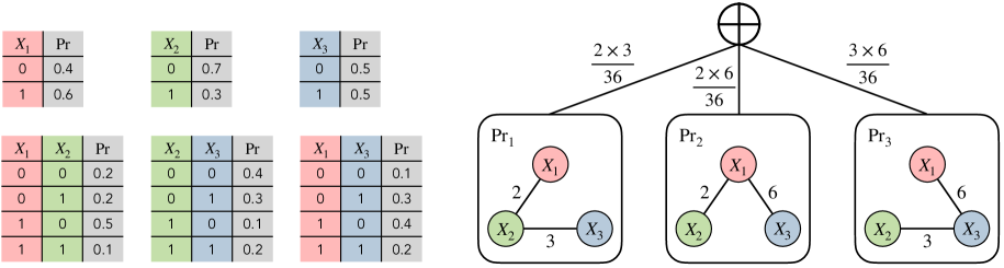
Figure 1: An example MoAT distribution over 3 binary random variables $X_{1},X_{2},\text{ and }X_{3}$. The summation at the top denotes a mixture distribution where the mixture weights are given by the weights of the corresponding spanning tree (shown on the edges). The tables on the left shows the univariate and pairwise marginal distributions, which are shared across the mixture components (3 possible spanning trees).

In this section, we propose mixture of all trees (MoAT) as a new class of probabilistic models. We first introduce tree-shaped Markov random fields (MRFs) and define the MoAT model as a mixture over all possible tree distributions weighted by the spanning tree distribution. Then, we demonstrate how to tractably compute normalized likelihood on the MoAT model.

2.1 Mixture of Tree-shaped Graphical Models

A tree-shaped MRF with underlying graph structure $G(V,E)$ represents a joint probability distribution ${\Pr}_{G}$ over $n$ random variables $\mathbf{X}=X_{1},\cdots,X_{n}$ by specifying their univariate and pairwise marginal distributions. Specifically, assuming $G$ is a tree with vertex set $V=\{1,\cdots,n\}$, we associate with each edge $(u,v)\in E$ a pairwise marginal distribution ${P}_{uv}(X_{u},X_{v})$ and each vertex $u$ a univariate marginal distribution ${P}_{v}(X_{v})$. Assuming that ${P}_{uv}$ and ${P}_{v}$ are consistent, then the normalized joint distribution ${\Pr}_{G}$ is given by meila-jordan:

$${\Pr}_{G}(\mathbf{x})=\frac{\prod_{(u,v)\in E}{{P}_{uv}(x_{u},x_{v})}}{\prod_{u\in V}{P}_{v}(x_{v})^{\deg v-1}},$$ (1)

where $\mathbf{x}\!=\!(x_{1},\cdots,x_{n})$ denotes assignment to $\mathbf{X}$ and $\deg{v}$ denotes the degree of $v$ in $G$; see $\Pr_{1}(X_{1},X_{2},X_{3})$ in Figure 1 as an example tree-shaped MRF.

Despite the tractability of tree-shaped MRFs, they suffer from the problem of limited expressive power. To improve the expressive power, prior works propose to learn mixtures of tree models (anandkumar2012learning, meila-jordan), where they focus on simple mixtures of a few trees, and propose EM algorithms for parameter and structure learning. This idea, however, suffers from several limitations. Firstly, while it is known how to optimally pick a single tree distribution with respect to the training data via the Chow-Liu algorithm (chow-liu), no known closed form solution exists for picking the optimal set of tree distributions as mixture components from the super-exponentially many possible choices for spanning trees. Secondly, by having a small fixed number of (even possibly optimal) mixture components, the model forces us to commit to a few sparse dependency structures that might not be capable of capturing complex dependencies anyway.

Though mixture of trees model becomes more expressive as more tree structures are included, the number of parameters increases with the number of mixture components, which seem to suggest that a mixture over a large number of tree components is infeasible. Despite this, we propose the mixture of all trees model (MoAT), a polynomial-size representation for the mixture over all possible (super-exponentially many) tree-shaped MRFs.

Formally, we define:

$${\Pr}_{\text{MoAT}}(\mathbf{x})=\frac{1}{Z}\sum_{T\in\text{ST}(K_{n})}\left(\prod_{e\in T}w_{e}\right){\Pr}_{T}(\mathbf{x})$$ (2)

where $K_{n}$ denotes the complete graph on $n$ vertices, $\mathsf{ST}(G)$ denotes the set of spanning trees of a connected graph $G$, and $Z$ is the normalization constant. Each mixture component is a tree-shaped MRF $\Pr_{T}$ weighted by $\prod_{e\in T}w_{e}$, that is, product of the edge weights of the tree. Note that we define the weight of each tree to be proportional to its probability in the spanning tree distribution (borcea2009negative), which is tractable, allowing for efficient likelihood computation on MoAT (Section 2.2.)

Though a MoAT model represents a mixture over super-exponentially many tree-shaped MRFs, the number of parameters in MoAT is polynomial-size due the the parameter sharing across its mixture components. Specifically, all tree-shaped MRFs $\Pr_{T}(\mathbf{x})$ share the same univariate and pair-wise marginals (i.e., $P_{u}(x_{u})$ and $P_{uv}(x_{u},x_{v})$); in addition, each edge in the graph $K_{n}$ is parameterized by a positive weight $w_{uv}$. To summarize, a MoAT model over $n$ variables has $O(n^{2})$ parameters.

Figure 1 shows an example MoAT model over 3 binary random variables $X_{1},X_{2},X_{3}$, for which there are $3$ possible spanning trees. Note that each of the mixture components (tree distributions) share the same set of marginals, but encode different distributions by virtue of their different dependency structures.

For example, for the distribution represented in Figure 1,

$${\Pr}_{\text{MoAT}}(X_{1}=1,X_{2}=0,X_{3}=1)$$

$$=\frac{1}{Z}\sum_{T\in\mathsf{ST}(K_{n})}\left(\prod_{e\in T}w_{e}\right)T(\mathbf{x})$$

$$=\frac{1}{2\times 3+3\times 6+6\times 2}\times[\left(2\times 3\times\frac{0.5\times 0.3}{0.7}\right)$$

$$\quad+\left(2\times 6\times\frac{0.5\times 0.2}{0.6}\right)+\left(3\times 6\times\frac{0.2\times 0.3}{0.5}\right)]$$

By Cayley’s formula (chaiken1978matrix), the number of spanning trees increases super-exponentially with respect to the number of random variables, thus preventing us from evaluating them by enumeration.

2.2 Tractable Likelihood for MoAT

Despite a super-exponential number ($n^{n-2}$) of mixture components, we show that computing (normalized) likelihood on MoAT is tractable. Our approach primarily leverages the tractability of spanning tree distributions and their compact representation as probability generating polynomials, which has been extensively studied in the context of machine learning (li2016fast, mariet2018exponentiated, robinson2019flexible, ZhangICML21).

Definition 1.

Let $\Pr(\cdot)$ be a probability distribution over $n$ binary random variables $\mathbf{X}\!=\!X_{1},X_{2},\dots,X_{n}$, then the probability generating polynomial for $\Pr$ is defined as

$${\sum}_{\mathbf{x}\in\{0,1\}^{n}}\Pr(\mathbf{X}=\mathbf{x})\left({\prod}_{i\text{ s.t. }x_{i}=1}z_{i}\right),$$

where each $z_{i}$ is an indeterminate associated with $X_{i}$.

To define spanning tree distributions and present their representation as probability generating polynomials, we first introduce some notation. Let $G=(V,E)$ be a connected graph with vertex set $V=\{1,\dots,n\}$ and edge set $E$. Associate to each edge $e\in E$ an indeterminate $z_{e}$ and a weight $w_{e}\in\mathbb{R}_{\geq 0}$. If $e=\{i,j\}$, let $A_{e}$ be the $n\times n$ matrix where $A_{ii}=A_{jj}=1$, $A_{ij}=A_{ji}=-1$ and all other entries equal to $0$. Then the weighted Laplacian of $G$ is given by $L(G)=\sum_{e\in E}w_{e}z_{e}A_{e},$

For instance, the weighted Laplacian for the example MoAT distribution in Figure 1 is

$$\begin{bmatrix}2z_{ab}+6z_{ac}&-2z_{ab}&-6z_{ac}\\ -2z_{ab}&2z_{ab}+3z_{bc}&-3z_{bc}\\ -6z_{ac}&-3z_{bc}&3z_{bc}+6z_{ac}\\ \end{bmatrix}$$

Using $L(G)_{\backslash\{i\}}$ to denote the principal minor of $L(G)$ that is obtained by removing its $i^{th}$ row and column, by the Matrix Tree Theorem (chaiken1978matrix), the probability generating polynomial for the spanning tree distribution is given by:

$$\operatorname{det}(L(G)_{\backslash\{i\}})=\sum_{T\in\mathsf{ST}(G)}\left(\prod_{e\in T}w_{e}z_{e}\right)$$ (3)

Now we derive the formula for computing ${\Pr}_{\text{MoAT}}(\mathbf{x})$ efficiently. We first set $G=K_{n}$ and $z_{e}=\frac{P_{uv}}{P_{u}P_{v}}$ and define:

$$L^{*}:=L(K_{n})_{\backslash\{i\}}\bigr{\rvert}_{z_{e}=\frac{P_{uv}}{P_{u}P_{v}}};$$

and it follows from Equation 3 that

$$\operatorname{det}\left(L^{*}\right)=\sum_{T\in\mathsf{ST}(K_{n})}\left(\prod_{e\in T}w_{e}\right)\prod_{(u,v)\in T}\frac{P_{uv}}{P_{u}P_{v}};$$

note that $\prod_{(u,v)\in T}P_{u}P_{v}=\prod_{u}P_{u}^{\text{deg}(u)}$; hence,

$$\operatorname{det}\left(L^{*}\right)\!=\!\frac{1}{\prod_{v\in V}P_{v}}\sum_{T\in\mathsf{ST}(K_{n})}\!\left(\prod_{e\in T}w_{e}\right)\!\frac{\prod_{(u,v)\in T}P_{uv}}{\prod_{v\in V}P_{v}^{\operatorname{deg}v-1}}$$

$$\quad\!=\!\frac{Z}{\prod_{v\in V}P_{v}}{\Pr}_{\text{MoAT}},$$

where the second equality follows from the definition of MoAT (Equation 2). Finally, we multiply both sides by $\left(\prod_{v\in V}P_{v}\right)/Z$ thus ${\Pr}_{\text{MoAT}}(\mathbf{x})$ can be evaluated as:

$${\Pr}_{\text{MoAT}}(\mathbf{x})=\frac{1}{Z}\left(\prod_{v\in V}P_{v}\left(x_{v}\right)\right)\operatorname{det}(L^{*}\bigr{\rvert}_{\mathbf{x}}).$$

Note that the normalization constant of the MoAT model $Z=\sum_{T\in\mathsf{ST}(K_{n})}\left(\prod_{e\in T}w_{e}\right)$ can be evaluated efficiently as a determinant by replacing the indeterminate $z_{e}$ with the constant 1. As the computational bottleneck is the determinant calculation, the time complexity is upper bounded as $\mathcal{O}(n^{\omega})$, where $\omega$ is the matrix multiplication exponent.

3 DENSITY ESTIMATION

In the previous section, we introduced the MoAT model and described how we can compute likelihood tractably. In this section, we describe how to parameterize the MoAT model in a way that is amenable to learning and subsequently effective density estimation on real world datasets. There are few desirable properties we seek from this parameterization (of univariate and pairwise marginals in particular). Firstly, we need to parameterize the marginals in way that are consistent with each other. This is essential as it guarantees that all tree-shaped mixture components (Equation 1) in the MoAT model are normalized. Secondly, we want our parameterization to capture the entire space of consistent combinations of univariate and pairwise marginals. In particular, this also ensures that every tree distribution is representable by our parameterization.

3.1 MoAT Parameter Learning

For a MoAT model over $n$ binary random variables $V=\{X_{1},X_{2},...,X_{n}\}$, we propose the following parameterization (as illustrated in Figure 2):

• Edge weights: $w_{e}\in\mathbb{R}_{\geq 0}$ for $e\in{V\choose 2}$.

• Univariate marginals: $p_{v}\!=\!P(X_{v}\!=\!1)\in[0,1]$ $\forall v\in V$.

• Pairwise marginals: $p_{uv}\!=\!P(X_{u}\!=\!1,X_{v}\!=\!1)\in[\max(0,p_{u}+p_{v}-1),\min(p_{u},p_{v})]$ for $\{u,v\}\in{V\choose 2}$.

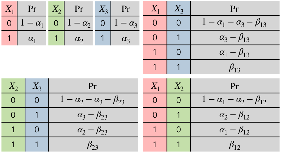
Figure 2: Parameterization for multivariate and univariate marginals for the example distribution on three binary random variables. The $\alpha_{i}$s and $\beta_{ij}$s are the free parameters.

As mentioned in Section 2, to ensure that all the mixture components of MoAT are normalized, our parameterization for $P_{u}$ and $P_{uv}$ needs to be consistent; specifically, they need to satisfy the following constraints:

• $P(X_{v}\!=0)+P(X_{v}\!=\!1)\!=\!1$ for all $v\in V$.

• $\sum_{a\in\{0,1\}}P(X_{u}\!=\!a,X_{v}\!=\!b)\!=\!P(X_{v}\!=b)\text{ }\forall b\in\{0,1\},\forall\{u,v\}\in{V\choose 2}$.

• $\sum_{(a,b)\in\{0,1\}^{2}}P(X_{u}\!=\!a,X_{v}\!=\!b)\!=\!1\text{ }\forall\{u,v\}\in{V\choose 2}$.

Lemma 1.

For any distribution $\Pr(\cdot)$ over binary random variables $X_{1},\dots,X_{n}$, there exists a set of parameters (i.e., $p_{v}$ and $p_{uv}$) in our hypothesis space such that $\Pr(X_{u})=P_{u}(X_{u})$ and $\Pr(X_{u},X_{v})=P_{uv}(X_{u},X_{v})$ for all $1\leq u,v\leq n$; i.e., the univariate and pair-wise marginals of $\Pr$ are the same as $P_{u}$ and and $P_{uv}$.

See appendix for proof. This lemma shows that the MoAT parameterization is not just valid, but also fully general in the sense that it covers all possible consistent combinations of univariate and pairwise marginals. Further, the MoAT parameterization naturally extends to categorical variables. For categorical random variables $V=\{X_{1},X_{2},...,X_{n}\}$, let $\mathsf{val}(X_{i})=\{1,2,\cdots,k_{i}\}$. It is easy to see that the values $P(X_{v}=i)$ for $i\in\{1,2,\cdots,k_{v}-1\}$ uniquely determine the univariate marginals. Similarly, the values $P(X_{u}\!=\!i,X_{v}\!=\!j)$ for $(i,j)\in\{1,2,\cdots,k_{u}-1\}\times\{1,2,\cdots,k_{v}-1\}$ uniquely determine the pairwise marginals. This extension is provably valid, but not fully general. For MoAT over categorical variables, whether there exists a fully general parameterization (i.e., Lemma 1 holds) is unknown. See appendix for a detailed discussion.

Parameter Learning

For individual tree distributions, the optimal tree structure (as measured by KL divergence from training data) is the maximum weight spanning tree of the complete graph, where edge weights are given by mutual information between the corresponding pairs of variables (chow-liu). Following this intuition, we use mutual information to initialize $w_{e}$; besides, we also initialize the univariate and pairwise marginals of the MoAT model by estimating them from training data. Finally, given our parameter initialization, we train the MoAT model by performing maximum likelihood estimation (MLE) via stochastic gradient descent.

It is worth noting that our parameter initialization is deterministic. We perform ablation studies to check the effectiveness of our initialization. As shown in Figure 3, compared to random initialization, we observe that our special initialization always leads to better initial log likelihood, faster convergence and better final log likelihood.

(a) NLTCS Dataset

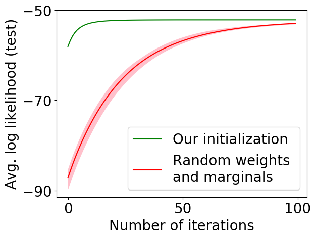
(b) Jester Dataset

Figure 3: Average log-likelihood throughout training on datasets across various data dimensionalities: our initialization vs. random initialization (averaged over 5 runs).

3.2 Density Estimation via MoAT

Dataset	# vars	MoAT	HCLT	MT
nltcs	16	-6.07	-5.99	-6.01
msnbc	17	-6.43	-6.05	-6.07
kdd	65	-2.13	-2.18	-2.13
plants	69	-13.50	-14.26	-12.95
baudio	100	-39.03	-39.77	-40.08
jester	100	-51.65	-52.46	-53.08
bnetflix	100	-55.52	-56.27	-56.74
accidents	111	-31.59	-26.74	-29.63
tretail	135	-10.81	-10.84	-10.83
pumsb	163	-29.89	-23.64	-23.71
dna	180	-87.10	-79.05	-85.14
kosarek	190	-10.57	-10.66	-10.62
msweb	294	-9.80	-9.98	-9.85
book	500	-33.46	-33.83	-34.63
tmovie	500	-49.37	-50.81	-54.60
cwebkb	839	-147.70	-152.77	-156.86
cr52	889	-84.78	-86.26	-85.90
c20ng	910	-149.44	-153.4	-154.24
bbc	1058	-243.82	-251.04	-261.84
ad	1556	-15.30	-16.07	-16.02

Table 1: Comparison of average log likelihood of MoAT, HCLT, and MT across the Twenty Datasets benchmarks. Best results are presented in bold.

We evaluate MoAT on a suite of density estimation datasets called the Twenty Datasets  (twenty-datasets), which contains 20 real-world datasets covering a wide range of application domains including media, medicine, and retail. This benchmark has been extensively used to evaluate tractable probabilistic models. We compare MoAT against two baselines: (1) hidden Chow-Liu trees (HCLTs) (hclt), which are a class of probabilistic models that achieve state-of-the-art performance on the Twenty Datasets benchmark and (2) the mixture of trees model (MT) (meila-jordan).

Table 1 summarizes the experiment results. MoAT outperforms both HCLT and MT on 14 out of 20 datasets. In particular, the MoAT model beats baselines by large margins on all datasets with more than 180 random variables. It is also worth noting that despite having fewer parameters ($\mathcal{O}(n^{2})$) than MT ($\mathcal{O}(k\cdot n^{2})$, where $k$ is the number of mixture components in MT), MoAT almost always outperforms MT, with the exception of a few smaller datasets, where MoAT does not have enough parameters to fit the data well.

4 ON THE HARDNESS OF MARGINALS AND MAP INFERENCE

In this section, we prove the hardness of semiring queries (which is a generalization of marginals) and Maximum a posteriori (MAP) inference on the MoAT model.

4.1 On the Hardness of Computing Marginals

First, we define the notion of semiring queries.

Definition 2.

Semiring Queries (SQ): Let $p(\mathbf{X})$ be a real-valued function over random variables $\mathbf{X}$. The class of semiring queries $\mathcal{Q}_{\mathrm{F}}$ is the set of queries that compute values of the following form:

$$f(\boldsymbol{e})= \sum_{\mathbf{z}}p(\mathbf{z},\boldsymbol{e})$$

where $e\in\mathrm{val}(\mathbf{E})$ is a partial configuration for any subset of random variables $\mathbf{E}\subseteq\mathbf{X}$, and $\mathbf{Z}=\mathbf{X}\backslash\mathbf{E}$ is the set of remaining random variables.

When the semiring sum/product operations correspond to the regular sum/product operations and the function $p$ is a likelihood function, the semiring query $f(\mathbf{e})$ actually computes marginal probabilities.

In fact, if $p$ is the likelihood function for the MoAT model, for an assignment $\mathbf{e}$ to $\mathbf{E}\subseteq\mathbf{X}$,

$$f(\boldsymbol{e})= \frac{1}{Z}\sum_{\mathbf{z}}\sum_{T\in\mathsf{ST}(K_{n})}\left(\prod_{v\in V}P_{v}\left(x_{v}\right)\right)$$

$$\left(\prod_{(u,v)\in T}w_{(u,v)}\frac{P_{uv}(x_{u},x_{v})}{P_{u}(x_{u})P_{v}(x_{v})}\right),$$

where $Z=\sum_{T\in\mathsf{ST}(K_{n})}\left(\prod_{e\in T}w_{e}\right)$ is the normalization constant and $\mathbf{z}$ enumerates over all instantiations of $\mathbf{Z}=\mathbf{X}\backslash\mathbf{E}$. Thus, in this case, $f(\mathbf{e})$ actually computes marginals in the MoAT model. However, the generality of the semiring queries allows for negative parameter values and hence negative “probabilities”, which we leverage to prove hardness of semiring queries on the MoAT model.

Since most marginal computation algorithms on tractable probabilistic models (such as the jointree algorithm which relies on variable elimination (ZhangPoole, Dechter1996) and circuit compilation based methods (chavira, darwiche2002factor)) are semiring generalizable (wachter, kimmig17, bacchus09), the hardness of semiring queries on the MoAT model would strongly suggest the hardness of marginal computation. In other words, the hardness of semiring queries would rule out most marginal inference techniques in the literature as they perform purely algebraic computations on the parameter values without any restrictions/assumptions on the range of these values. We dedicate the rest of this subsection to establishing the same, while deferring most technical proof details to the appendix.