PointFlowHop: Green and Interpretable Scene Flow Estimation from Consecutive Point Clouds

Abstract

An efficient 3D scene flow estimation method called PointFlowHop is proposed in this work. PointFlowHop takes two consecutive point clouds and determines the 3D flow vectors for every point in the first point cloud. PointFlowHop decomposes the scene flow estimation task into a set of subtasks, including ego-motion compensation, object association and object-wise motion estimation. It follows the green learning (GL) pipeline and adopts the feedforward data processing path. As a result, its underlying mechanism is more transparent than deep-learning (DL) solutions based on end-to-end optimization of network parameters. We conduct experiments on the stereoKITTI and the Argoverse LiDAR point cloud datasets and demonstrate that PointFlowHop outperforms deep-learning methods with a small model size and less training time. Furthermore, we compare the Floating Point Operations (FLOPs) required by PointFlowHop and other learning-based methods in inference, and show its big savings in computational complexity.

Keywords 3D scene flow estimation  $\cdot$ green learning  $\cdot$ unsupervised learning  $\cdot$ PointHop

1 Introduction

Dynamic 3D scene understanding based on captured 3D point cloud data is a critical enabling technology in the 3D vision systems. 3D scene flow aims at finding the point-wise 3D displacement between consecutive point cloud scans. With the increase in the availability of point cloud data, especially those acquired via the LiDAR scanner, 3D scene flow estimation directly from point clouds is an active research topic nowadays. 3D scene flow estimation finds rich applications in 3D perception tasks such as semantic segmentation, action recognition, and inter-prediction in compressing sequences of LiDAR scans.

Today’s solutions to 3D scene flow estimation mostly rely on supervised or self-supervised deep neural networks (DNNs) that learn to predict the point-wise motion field from a pair of input point clouds via end-to-end optimization. One of the important components of these methods is to learn flow embedding by analyzing spatio-temporal correlations among regions of the two point clouds. After the successful demonstration of such an approach in FlowNet3D [1], there has been an increased number of papers on this topic by exploiting and combining other ideas such as point convolutions and attention mechanism.

These DNN-based methods work well in an environment that meets the local scene rigidity assumption. They usually outperform classical point-correspondence-based methods. On the other hand, they have a large number of parameters and rely on large training datasets. For the 3D scene flow estimation problem, it is non-trivial to obtain dense point-level flow annotations. Thus, it is challenging to adopt the heavily supervised learning paradigm with the real world data. Instead, methods are typically trained on synthetic datasets with ground truth flow information first. They are later fine-tuned for real world datasets. This makes the training process very complicated.

In this paper, we develop a green and interpretable 3D scene flow estimation method for the autonomous driving scenario and name it “PointFlowHop”. We decompose our solution into vehicle ego-motion and object motion modules. Scene points are classified as static and moving. Moving points are grouped into moving objects and a rigid flow model is established for each object. Furthermore, the flow in local regions is refined assuming local scene rigidity. PointFlowHop method adopts the green learning (GL) paradigm [2]. It is built upon related recent work, GreenPCO [3], and preceding foundation works such as R-PointHop [4], PointHop [5], and PointHop++ [6].

The task-agnostic nature of the feature learning process in prior art enables scene flow estimation through seamless modification and extension. Furthermore, a large number of operations in PointFlowHop are not performed during training. The ego-motion and object-level motion is optimized in inference only. Similarly, the moving points are grouped into objects only during inference. This makes the training process much faster and the model size very small. The decomposition of 3D scene flow into object-wise rigid motion and/or ego-motion components is not entirely novel. However, our focus remains in developing a GL-based solution with improved overall performance, including accuracy, model sizes and computational complexity.

The novelty of our work lies in two aspects. First, it expands the scope of existing GL-based point cloud data processing techniques. GL-based point cloud processing has so far been developed for object-level understanding [7, 8, 9, 10, 6, 5] and indoor scene understanding [4, 11]. This work addresses the more challenging problem of outdoor scene understanding at the point level. This work also expands the application scenario of R-PointHop, where all points are transformed using one single rigid transformation. For 3D scene flow estimation, each point has its own unique flow vector. Furthermore, we show that a single model can learn features for ego-motion estimation as well as object-motion estimation, which are two different but related tasks. This allows model sharing and opens doors to related tasks such as joint scene flow estimation and semantic segmentation. Second, our work highlights the over-paramertized nature of DL-based solutions which demand larger model sizes and higher computational complexity in both training and testing. The overall performance of PointFlowHop suggests a new point cloud processing pipeline that is extremely lightweight and mathematically transparent.

To summarize, there are three major contributions of this work.

• We develop a lightweight 3D scene classifier that identifies moving points and further clusters and associates them into moving object pairs.

• We optimize the vehicle ego-motion and object-wise motion based on point features learned using a single task-agnostic feedforward PointHop++ model.

• PointFlowHop outperforms representative benchmark methods in the scene flow estimation task on two real world LiDAR datasets with fewer model parameters and lower computational complexity measured by FLOPs (floating-point operations).

The rest of the paper is organized as follows. Related work is reviewed in Sec. 2. The PointFlowHop method is proposed in Sec. 3. Experimental results are presented in Sec. 4. Finally, concluding remarks and possible future extensions are given in Sec. 5.

2 Related Work

2.1 Scene Flow Estimation

Early work on 3D scene flow estimation uses 2D optical flow estimation followed by triangulation such as that given in [12]. The Iterative Closest Point (ICP) [13] and the non-rigid registration work, NICP [14], can operate on point clouds directly. Series of image- and point-based seminal methods for scene flow estimation relying on similar ideas were proposed in the last two decades. The optical flow is combined with dense stereo matching for flow estimation in [15]. A variational framework that predicts the scene flow and depth is proposed in [16]. A peicewise rigid scene flow estimation method is investigated in [17]. Similarly, the motion of rigidly moving 3D objects is examined in [18]. Scene flow based on Lucas-Kanade tracking [19] is studied in [20]. An exhaustive survey on 2D optical flow and 3D scene flow estimation methods has been done by Zhai et al. [21].

Deep-learning-based (DL-based) methods have been popular in the field of computer vision in the last decade. For DL-based 3D scene flow estimation, FlowNet3D [1] adopts the feature learning operations from PointNet++ [22]. HPLFlowNet [23] uses bilateral convolution layers and projects point clouds to an ordered permutohedral lattice. PointPWC-Net [24] takes a self-supervised learning approach that works in a coarse-to-fine manner. FLOT [25] adopts a correspondence-based approach based on optimal transport. HALFlow [26] uses a hierarchical network structure with an attention mechanism. The Just-Go-With-the-Flow method [27] uses self-supervised learning with the nearest neighbor loss and the cycle consistency loss.

DL-based methods that attempt to simplify the flow estimation problem using ego-motion and/or object-level motion have also been investigated. For example, Rigid3DSceneFlow [28] reasons the scene flow at the object level (rather than the point level). Accordingly, the flow of scene background is analyzed via ego-motion and that of a foreground object is described by a rigid model. RigidFlow [29] enforces the rigidity constraint in local regions and performs rigid alignment in each region to produce rigid pseudo flow. SLIM [30] uses a self-supervised loss function to separate moving and stationary points.

2.2 Green Point Cloud Learning

Green Learning (GL) [2] has started to gain attention as an alternative to Deep Learning (DL) in recent years. Typcially, GL consists of three modules: 1) unsupervised representation learning, 2) supervised feature learnaing, and 3) supervised decision learning. The unsupervised representation learning in the first module is rooted in the derivation of data-driven transforms such as the Saak [31] and the Saab [32] transforms. Both the training and inference processes in GL adopt a feedforward data processing path without backpropagation. The optimization is statistics-based, and it is carried out at each module independently. The learning process is lightweight, making it data and computation resource friendly. GL-based methods have been developed for a wide variety of image processing and computer vision tasks [2].

Green Point Cloud learning [33] was first introduced in PointHop [5]. The unsupervised representation learning process involves constructing a local point descriptor via octant space partitioning followed by dimensionality reduction via the Saab transform. These operations together are called one PointHop unit. It is the fundamental building block in series of follow-up works along with other task-specific modules. PointHop++ [6] replaces the Saab transform with its efficient counterpart called the Channel-wise Saab transform [34]. PointHop and PointHop++ adopt a multi-hop learning system for point cloud classification, whereby the learned point representations are aggregated into a global feature vector and fed to a classifier. The multi-hop learning architecture is analogous to the hierarchical deep learning architecture. The multi-hop architecture helps capture the information from short-, mid-, and long-range point cloud neighborhoods.

More recently, R-PointHop [4], GSIP [11] and GreenPCO [3] demonstrate green learning capabilities on more challenging large-scale point clouds for indoor scene registration, indoor segmentation, and odometry tasks, respectively. R-PointHop finds corresponding points between the source and target point clouds using the learned representations and then estimates the 3D rotation and translation to align the source with the target. In GreenPCO, a similar process is adopted to incrementally estimate the object’s trajectory. Additional ideas presented in GreenPCO include a geometry-aware point cloud sampling scheme that is suitable for LiDAR data. Other noteworthy green point cloud learning works include SPA [8], UFF [10], PCRP [9], and S3I-PointHop [7].

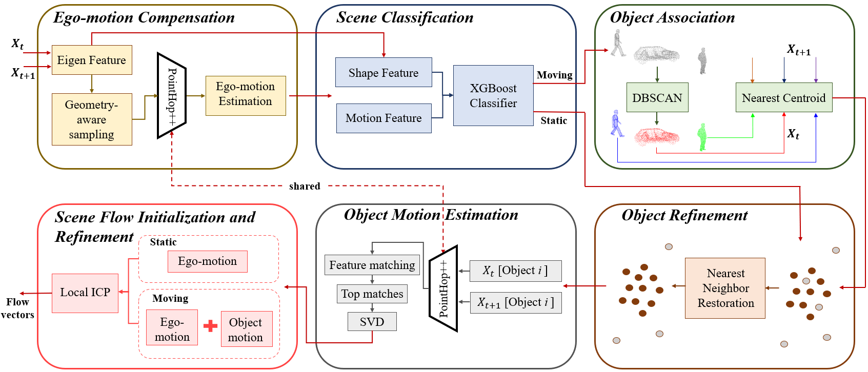
Figure 1: An overview of the PointFlowHop method, which consists of six modules: 1) ego-motion compensation, 2) scene classification, 3) object association, 4) object refinement, 5) object motion estimation, and 6) scene flow initialization and refinement.

3 Proposed PointFlowHop Method

The system diagram of the proposed PointFlowHop method is shown in Fig. 1. It takes two consecutive point clouds $X_{t}\in\mathbb{R}^{n_{t}\times 3}$ and $X_{t}\in\mathbb{R}^{n_{t+1}\times 3}$ as the input and calculates the point-wise flow $\bar{f_{t}}\in\mathbb{R}^{n_{1}\times 3}$ for the points in $X_{t}$.

PointFlowHop decomposes the scene flow estimation problem into two subproblems: 1) determining vehicle’s ego-motion $(T_{ego})$ and 2) estimating the motion of each individual object (denoted by $(T_{obj_{i}})$ for object $i$). It first proceeds by determining and compensating the ego-motion and classifying scene points as being moving or static in modules 1 and 2, respectively. Next, moving points are clustered and associated as moving objects in modules 3 and 4, and the motion of each object is estimated in module 5. Finally, the flow vectors of static and moving points are jointly refined. These steps are detailed below.

3.1 Module 1: Ego-motion Compensation

The $i^{th}$ point in $X_{t}$ has coordinates $(x_{t}^{i},y_{t}^{i},z_{t}^{i})$. Suppose this point is observed at $(x_{t+1}^{i},y_{t+1}^{i},z_{t+1}^{i})$ in $X_{t+1}$. These point coordinates are expressed in the respective LiDAR coordinate systems centered at the vehicle position at time $t$ and $t+1$. Since the two coordinate systems may not overlap due to vehicle’s motion, the scene flow vector, $\bar{f_{t}}^{i}$, of the $i^{th}$ point cannot be simply calculated using vector difference. Hence, we begin by aligning the two coordinates systems or, in other words, we compensate for the vehicle motion (or called ego-motion).

The ego-motion compensation module in PointFlowHop is built upon a recently proposed point cloud odometry estimation method, called GreenPCO [3]. It is briefly reviewed below for self-containedness. GreenPCO determines the vehicle trajectory incrementally by analyzing consecutive point cloud scans. It is conducted with the following four steps. First, the two point clouds are sampled using the geometry-aware sampling method, which selects points spatially spread out with salient local surfaces based on the eigen features [35]. Second, the sampled points from the two point clouds are divided into four views - front, left, right and rear based on the azimuthal angles. Third, point features are extracted using PointHop++ [6]. The features are used to find matching points between the two point clouds in each view. Last, the pairs of matched points are used to estimate the vehicle trajectory. These steps are repeated as the vehicle advances in the environment. The diagram of the GreenPCO method is depicted in Fig. 2.

Ego-motion estimation in PointFlowHop involves a single iteration of GreenPCO whereby the vehicle’s motion from time $t$ to $t+1$ is estimated. Then, the ego-motion can be represented by the 3D transformation, $T_{ego}$, which consists of a 3D rotation and 3D translation. Afterward, we use $T_{ego}$ to warp $X_{t}$ to $\tilde{X}_{t}$, making it in the same coordinate system as that of $X_{t+1}$. Then, the flow vector can be computed by

$$\bar{f_{t}}^{i}=(x_{t+1}^{i}-\tilde{x}_{t}^{i},y_{t+1}^{i}-\tilde{y}_{t}^{i},z_{t+1}^{i}-\tilde{z}_{t}^{i}),$$ (1)

where $(\tilde{x}_{t}^{i},\tilde{y}_{t}^{i},\tilde{z}_{t}^{i})$ is the warped coordinate of the $i^{th}$ point.

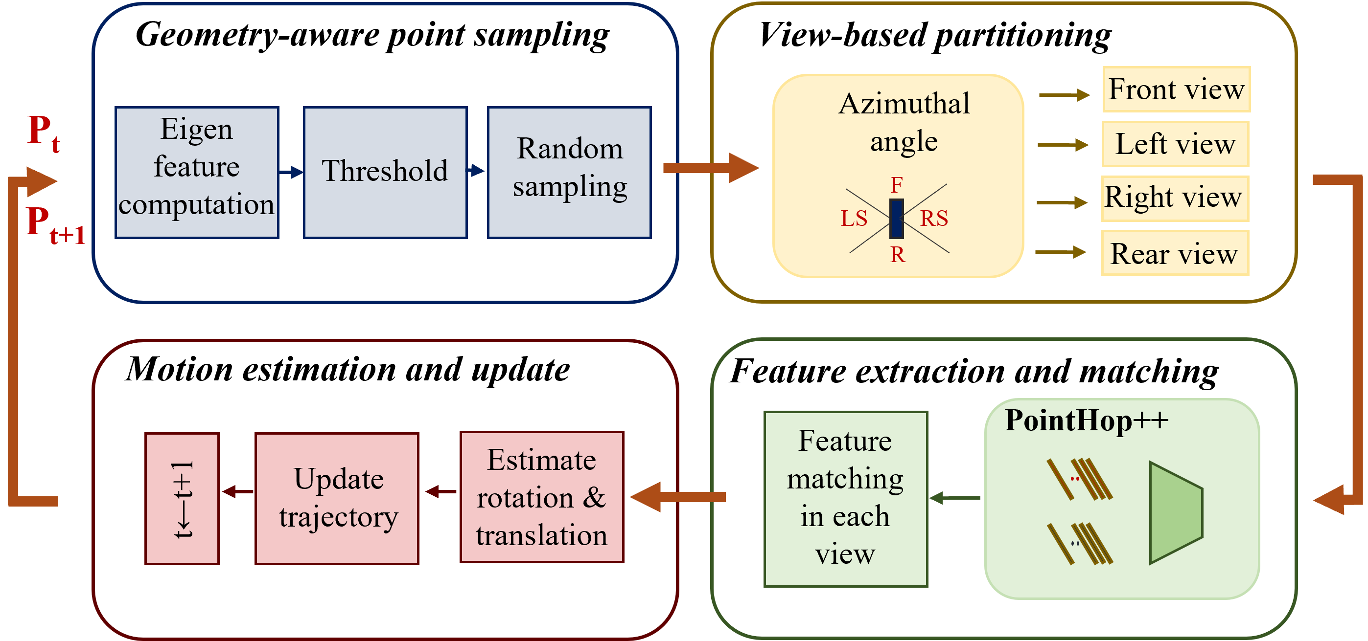
Figure 2: An overview of the GreenPCO method [3].

3.2 Module 2: Scene Classification

After compensating for ego-motion, the resulting $\tilde{X}_{t}$ and $X_{t+1}$ are in the same coordinate system (i.e., that of $X_{t+1}$). Next, we coarsely classify scene points in $\tilde{X}_{t}$ and $X_{t+1}$ into moving and static two classes. Generally speaking, the moving points may belong to objects such as cars, pedestrians, mopeds, etc., while the static points correspond to objects like buildings, poles, etc. The scene flow of moving points can be analyzed later while static points can be assigned a zero flow (or equal to the ego-motion depending on the convention of the coordinate systems used). This means that the later stages of PointFlowHop would process fewer points.

For the scene classifier, we define a set of shape and motion features that are useful in distinguishing static and moving points. These features are explained below.

• Shape features
  We reuse the eigen features [35] calculated in the ego-motion estimation step. They summarize the distribution of neighborhood points using covariance analysis. The analysis provides a 4-dimensional feature vector comprising of linearity, planarity, eigen sum and eigen entropy.

• Motion feature
  We first voxelize $\tilde{X}_{t}$ and $X_{t+1}$ with a voxel size of 2 meters. Then, the motion feature for each point in $\tilde{X}_{t}$ is the distance to the nearest voxel center in $X_{t+1}$, and vice versa, for each point in $X_{t+1}$.

The 5-dimensional (shape and motion) feature vector is fed to a binary XGBoost classifier. For training, we use the point-wise class labels provided by the SemanticKITTI [36] dataset. We observe that the 5D shape/motion feature vector are sufficient for decent classification. The classification accuracy on the SemanticKITTI dataset is 98.82%. Furthermore, some of misclassified moving points are reclassified in the subsequent object refinement step.

3.3 Module 3: Object Association

We simplify the problem of motion analysis on moving points by grouping moving points into moving objects. To discover objects from moving points, we use the Density-based Spatial Clustering for Applications with Noise (DBSCAN) [37] algorithm. Simply speaking, DBSCAN iteratively clusters points based on the minimum distance ($eps$) and the minimum points ($minPts$) parameters. Parameter $eps$ gives the minimum Euclidean distance between points considered as neighbors. Parameter $minPts$ determines the minimum number of points to form a cluster. Some examples of the objects discovered using PointFlowHop are colored in Fig. 3.

Points belonging to distinct objects may get clustered together. We put the points marked as “outliers” by DBSCAN in the set of static points. The DBSCAN algorithm is run on $\tilde{X}_{t}$ and $X_{t+1}$ separately. Later, we use cluster centroids to associate objects between $\tilde{X}_{t}$ and $X_{t+1}$. That is, for each centroid in $\tilde{X}_{t}$, we locate its nearest centroid in $X_{t+1}$.

3.4 Module 4: Object Refinement

Next, we perform an additional refinement step to recover some of the misclassified points during shape classification and potential inlier points during object association. This is done using the nearest neighbor rule within a defined radius neighborhood. For each point classified as a moving point, we re-classify static points lying within the neighborhood as moving points. The object refinement operation is conducted on $\tilde{X}_{t}$ and $X_{t+1}$.

The refinement step is essential for two reasons. First, an imbalance class distribution between static and moving points usually leads to the XGBoost classifier to favor the dominant class (which is the static points). Then, the precision and recall for moving points are still low in spite of high classification accuracy. Second, in the clustering step, it is difficult to select good values for $eps$ and $minPts$ that are robust in all scenarios for the sparse LiDAR point clouds. This may lead to some points being marked as outliers by DBSCAN. Overall, the performance gains of our method reported in Sec. 4 are a result of the combination of all steps and not due to a single step in particular.

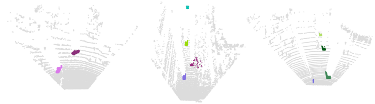
Figure 3: Objects clustered using the DBSCAN algorithm are shown in different colors.

3.5 Module 5: Object Motion Estimation

We determine the motion between each pair of associated objects in this step. For that, we follow a similar approach as taken by a point cloud rigid registration method, R-PointHop [4]. The objective of R-PointHop is to register the source point cloud with the target point cloud. The block diagram of R-PointHop is illustrated in Fig. 4. It includes the following two major steps. First, the source and target point clouds are fed to a sequence of R-PointHop units for hierarchical feature learning (or multiple hops) in the feature learning step. Point clouds are downsampled between two hops by iteratively selecting farther points. The R-PointHop unit comprises of constructing a local point descriptor followed by the channel-wise Saab transform [34]. Second, the point features are used to find pairs of corresponding points. The optimal rigid transformation that aligns the two point clouds is then solved as a energy minimization problem [38].

For object motion estimation in PointFlowHop, the features of refined moving points from $\tilde{X}_{t}$ and $X_{t+1}$ are extracted using the trained PointHop++ model. We reuse the same model from the ego-motion estimation step here. While four hops with intermediate downsampling is used in R-PointHop, the PointHop++ model in PointFlowHop only involves two hops without downsampling to suit the LiDAR data. Since $\tilde{X}_{t}^{obj_{i}}$ and $X_{t+1}^{obj_{i}}$ are two sets of points belonging to object $i$, we find corresponding points between the two point clouds using the nearest neighbor search in the feature space. The correspondence set is further refined by selecting top correspondences based on: 1) the minimum feature distance criterion and 2) the ratio test (the minimum ratio of the distance between the first and second best corresponding points). The refined correspondence set is then used to estimate the object motion as follows.

First, the mean coordinates of the corresponding points in $\tilde{X}_{t}^{obj_{i}}$ and $X_{t+1}^{obj_{i}}$ are found by:

$$\bar{x}_{t}^{obj_{i}}=\frac{1}{N_{obj_{i}}}\sum\limits_{j=1}^{N_{obj_{i}}}\tilde{x}_{t}^{obj_{ij}},\quad\bar{x}_{t+1}^{obj_{i}}=\frac{1}{N_{obj_{i}}}\sum\limits_{j=1}^{N_{obj_{i}}}x_{t+1}^{obj_{ij}}.$$ (2)

Then, the $3\times 3$ covariance matrix is computed using the pairs of corresponding points as

$$K(\tilde{X}_{t}^{obj_{i}},X_{t+1}^{obj_{i}})=\sum\limits_{j=1}^{N_{obj_{i}}}(\tilde{x}_{t}^{obj_{ij}}-\bar{x}_{t}^{obj_{i}})(x_{t+1}^{obj_{ij}}-\bar{x}_{t+1}^{obj_{i}})^{T}.$$ (3)

The Singular Value Decomposition of $K$ gives matrices $U$ and $U$, which are formed by the left and right singular vectors, respectively. Mathematically, we have

$$K(\tilde{X}_{t}^{obj_{i}},X_{t+1}^{obj_{i}})=USV^{T}.$$ (4)

Following the orthogonal procrustes formulation [38], the optimal motion of $\tilde{X}_{t}^{obj_{i}}$ can be expressed in form of a rotation matrix $R^{obj_{i}}$ and a translational vector $t^{obj_{i}}$. They can be computed as

$$R^{obj_{i}}=VU^{T},\quad t^{obj_{i}}=-R^{obj_{i}}\bar{x}_{t}^{obj_{i}}+\bar{x}_{t+1}^{obj_{i}}.$$ (5)

Since $(R^{obj_{i}},t^{obj_{i}})$ form the object motion model for object $i$, it is denoted as $T_{obj_{i}}$.

Actually, once we find the corresponding point $x_{t+1}^{obj_{ij}}$ of $\tilde{x}_{t}^{obj_{ij}}$, the flow vector may be set to

$$\tilde{x}_{t}^{obj_{ij}}=x_{t+1}^{obj_{ij}}-\tilde{x}_{t}^{obj_{ij}}.$$

However, this point-wise flow vector can be too noisy, and it is desired to use a flow model for the object rather than each point. The object flow model found using SVD in the step after finding correspondences is optimal in the mean square sense over all corresponding points and, hence, is more robust. It makes a reasonable assumption of existence of a rigid transformation between the two objects.

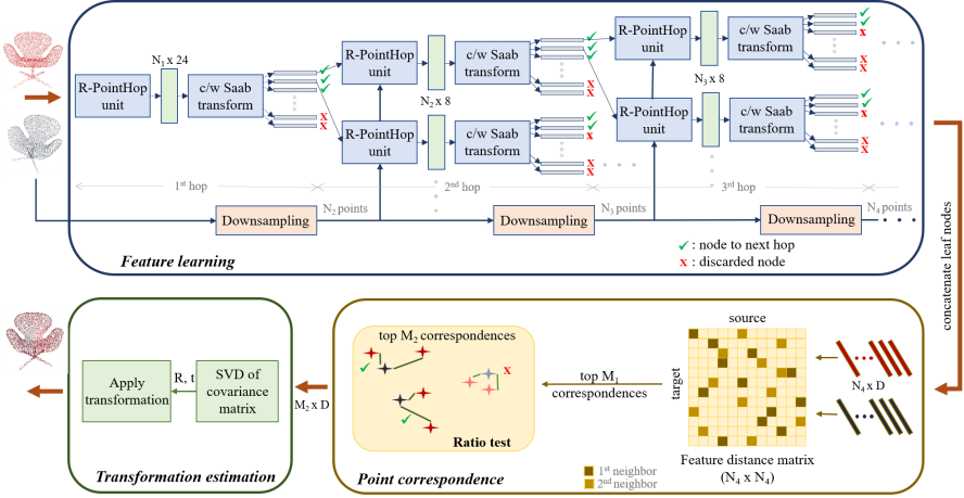
Figure 4: An overview of the R-PointHop method [4].

3.6 Module 6: Flow Initialization and Refinement

In the last module, we apply the object motion model $T_{obj_{i}}$ to $\tilde{X}_{t}^{obj_{i}}$ and align it with ${X}_{t+1}^{obj_{i}}$. Since the static points do not have any motion, they are not further transformed. We denote the new transformed point cloud as $\tilde{X}_{t}^{\prime}$. At this point, we have obtained an initial estimate of the scene flow for each point in $X_{t}$. For static points, the flow is given by the ego-motion transformation $T_{ego}$. For the moving points, it is a composition of ego motion and corresponding object’s motion $T_{ego}\cdot T_{obj_{i}}$.

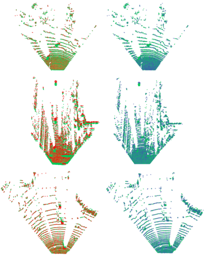
Figure 5: Flow estimation results using PointFlowHop: input point clouds (left) and warped output using flow vectors (right).

In this module, we refine the flow for all points in $\tilde{X}_{t}^{\prime}$ using the Iterative Closest Point (ICP) [13] algorithm in small non-overlapping regions. In each region, the points in $\tilde{X}_{t}^{\prime}$ falling within it are aligned with corresponding points in ${X}_{t+1}$. The flow refinement step ensures a tighter alignment and is a common post processing operation in several related tasks. Finally, the flow vectors for ${X}_{t}$ are calculated as difference between the transformed and initial coordinates. Exemplar pairs of input and scene flow compensated point clouds using PointFlowHop are shown in Fig. 5.

4 Experiments

In this section, we report experimental results on real world LiDAR point cloud datasets. We choose the stereoKITTI [39, 40] and the Argoverse [41] two datasets since they represent challenging scenes in autonomous driving environments. StereoKITTI has 142 pairs of point clouds. The ground truth flow of each pair is derived from the 2D disparity maps and the optical flow information. There are 212 test samples for Argoverse whose flow annotations were given in [42]. We use per-point labels from the SemanticKITTI dataset [36] to train our scene classifier.

Following series of prior art, we measure the performance in the following metrics:

• 3D end point error (EPE3D). It is the mean Euclidean distance between the estimated and the ground truth flow.

• Strict accuracy (Acc3DS). It is the percentage of points for which EPE3D is less than 0.05m or the relative error is less than 0.05.

• Relaxed accuracy (Acc3DR). It gives the ratio of points for which EPE3D is less than 0.1m or the relative error is less than 0.1.

• Percentage of Outliers. It is the ratio of points for which EPE3D is greater than 0.3m or the relative error is greater than 0.1. This is reported for the StereoKITTI dataset only.

• Mean angle error (MAE). It is the mean of the angle errors between the estimated and the ground truth flow of all points expressed in the unit of radians. This is reported for the Argoverse dataset only.

4.1 Performance Benchmarking

The scene flow estimation results on stereoKITTI and Argoverse are reported in Table 1 and Table 2, respectively. For comparison, we show the performance of several representative methods proposed in the past few years. Overall, the EPE3D, Acc3DS and Acc3DR values are significantly better for stereoKITTI as compared to the Argoverse dataset. This is because Argoverse is a more challenging dataset. Furthermore, PointFlowHop outperforms all benchmarking methods in almost all evaluation metrics on both datasets.

Table 1: Comparison of scene flow estimation results on the Stereo KITTI dataset, where the best performance number is shown in boldface.

Method	EPE3D (m)$\downarrow$	Acc3DS $\uparrow$	Acc3DR $\uparrow$	Outliers $\downarrow$
FlowNet3D [1]	0.177	0.374	0.668	0.527
HPLFlowNet [23]	0.117	0.478	0.778	0.410
PointPWC-Net [24]	0.069	0.728	0.888	0.265
FLOT [25]	0.056	0.755	0.908	0.242
HALFlow [26]	0.062	0.765	0.903	0.249
Rigid3DSceneFlow [28]	0.042	0.849	0.959	0.208
PointFlowHop (Ours)	0.037	0.938	0.974	0.189

Table 2: Comparison of scene flow estimation results on the Argoverse dataset, where the best performance number is shown in boldface.

Method	EPE3D (m) $\downarrow$	Acc3DS $\uparrow$	Acc3DR $\uparrow$	MAE (rad) $\downarrow$
FlowNet3D [1]	0.455	0.01	0.06	0.736
PointPWC-Net [24]	0.405	0.08	0.25	0.674
Just Go with the Flow [27]	0.542	0.08	0.20	0.715
NICP [14]	0.461	0.04	0.14	0.741
Graph Laplacian [42]	0.257	0.25	0.48	0.467
Neural Prior [43]	0.159	0.38	0.63	0.374
PointFlowHop (Ours)	0.134	0.39	0.71	0.398

4.2 Ablation Study

In this section, we assess the role played by each individual module of PointFlowHop using the stereo KITTI dataset as an example.

Ego-motion compensation. First, we may replace GreenPCO [3] with ICP [13] for ego-motion compensation. The results are presented in Table 3. We see a sharp decline in performance with ICP. The substitution makes the new method much worse than all benchmarking methods. While the naive ICP could be replaced with other advanced model-free methods, it is preferred to use GreenPCO since the trained PointHop++ model is still needed later.

Table 3: Ego-motion compensation – ICP vs. GreenPCO.

Ego-motion Method	EPE3D $\downarrow$	Acc3DS $\uparrow$	Acc3DR $\uparrow$	Outliers $\downarrow$
ICP [13]	0.574	0.415	0.481	0.684
GreenPCO [3]	0.037	0.938	0.974	0.189

Table 4: Performance gain due to object refinement.

Object Refinement	EPE3D $\downarrow$	Acc3DS $\uparrow$	Acc3DR $\uparrow$	Outliers $\downarrow$
✗	0.062	0.918	0.947	0.208
✓	0.037	0.938	0.974	0.189

Table 5: Performance gain due to flow refinement.

Flow Refinement	EPE3D $\downarrow$	Acc3DS $\uparrow$	Acc3DR $\uparrow$	Outliers $\downarrow$
✗	0.054	0.862	0.936	0.230
✓	0.037	0.938	0.974	0.189

Performance Gain Due to Object Refinement. Next, we compare PointFlowHop with and without the object refinement step. The results are shown in Table 4. We see consistent performance improvement in all evaluation metrics with the object refinement step. On the other hand, the performance of PointFlowHop is still better than that of benchmarking methods except for Rigid3DSceneFLow [28] (see Table 1) even without object refinement.

Performance Gain Due to Flow Refinement. Finally, we compare PointFlowHop with and without the flow refinement step in Table 5. It is not surprising that flow refinement is crucial in PointFlowHop. However, one may argue the refinement step may be included in any of the discussed methods as a post processing operation. While this argument is valid, we see that even without flow refinement, PointFlowHop still is better than almost all methods (see Table 1). Between object refinement and flow refinement, flow refinement seems slightly more important if we consider all four evaluation metrics jointly.

4.3 Complexity Analysis

The complexity of a machine learning method can be examined from multiple angles, including training time, the number of model parameters (i.e., the model size) and the number of floating point operations (FLOPs) during inference. These metrics are valuable besides performance measures such as prediction accuracy/error. Furthermore, since some model-free methods (e.g., LOAM [44]) and the recently proposed KISS-ICP [45] can offer state-of-the-art results for related tasks such as Odometry and Simultaneous Localization and Mapping (SLAM), the complexity of learning-based methods deserves additional attention.

To this end, PointFlowHop offers impressive benefits as compared to representative DL-based solutions. Training in PointFlowHop only involves the ego-motion compensation and shape classification steps. For object motion estimation, PointHop++ obtained from the ego-motion compensation step is reused while the rest of the operations in PointFlowHop are parameter-free and performed only in inference.

Table 6 provides details about the number of parameters of PointFlowHop. It adopts the PointHop++ architecture with two hops. The first hop has 13 kernels of dimension 88 while the second hop has 104 kernels of dimension 8. For XGBoost, it has 100 decision tree estimators, each of which has a maximum depth of 3. We also report the training time of PointFlowHop in the same table, where the training is conducted on Intel(R) Xeon(R) CPU E5-2620 v3 at 2.40GHz.

Table 6: The number of trainable parameters and training time of the proposed PointFlowHop.

	Number of Parameters	Training time
Hop 1	1144	20 minutes
Hop 2	832
XGBoost	2200	12 minutes
Total	4176	32 minutes

While we do not measure the training time of other methods ourselves, we use [42] as a reference to compare our training time with others. It took the authors of [42] about 18 hours to train and fine-tune the FlowNet3D [1] method for the KITTI dataset and about 3 days for the Argoverse dataset. We expect comparable time for other methods. Thus, PointFlowHop is extremely efficient in this context. While the Graph Laplacian method [42] offers a variant where the scene flow is entirely optimized at runtime (non-learning based), its performance is inferior to ours as shown in Table 2.

Table 7: Comparison of model sizes (in terms of the number of parameters) and computational complexity of inference (in terms of FLOPs) of four benchmarking methods.

Method	Number of Parameters	FLOPs
FlowNet3D [1]	1.23 M (308X)	11.67 G (61X)
PointPWC Net [24]	7.72 M (1930X)	17.46 G (92X)
FLOT [25]	110 K (28X)	54.65 G (288X)
PointFlowHop (Ours)	4 K (1X)	190 M (1X)

Finally, we compare the model sizes and computational complexity of four benchmarking methods in Table 7. It is apparent that PointFlowHop demands significantly less parameters than other methods. Furthermore, we compute the number of floating-point operations (FLOPs) of PointFlowHop analytically during inference and report it in Table 7. While calculating the FLOPs, we consider input point clouds containing 8,192 points. Thus, the normalized FLOPs per point is 23.19K. We conclude from the above discussion that PointFlowHop offers a green and high-performance solution to 3D scene flow estimation.

5 Conclusion and Future Work

A green and interpretable 3D scene flow estimation method called PointFlowHop was proposed in this work. PointFlowHop takes two consecutive LiDAR point cloud scans and determines the flow vectors for all points in the first scan. It decomposes the flow into vehicle’s ego-motion and the motion of an individual object in the scene. The superior performance of PointFlowHop over benchmarking DL-based methods was demonstrated on stereoKITTI and Argoverse datasets. Furthermore, PointFlowHop has advantages in fewer trainable parameters and fewer FLOPs during inference.

One future research direction is to extend PointFlowHop for the 3D object detection task. Along this line, we may detect moving objects using PointFlowHop and derive 3D bounding boxes around them. The clustered points obtained by PointFlowHop may act as an initialization in the object detection process. Another interesting problem to pursue is simultaneous flow estimation and semantic segmentation. The task-agnostic nature of our representation learning can be useful.

References

- [1] Xingyu Liu, Charles R Qi, and Leonidas J Guibas. Flownet3d: Learning scene flow in 3d point clouds. In Proceedings of the IEEE/CVF Conference on Computer Vision and Pattern Recognition, pages 529–537, 2019.
- [2] C-C Jay Kuo and Azad M Madni. Green learning: Introduction, examples and outlook. Journal of Visual Communication and Image Representation, page 103685, 2022.
- [3] Pranav Kadam, Min Zhang, Jiahao Gu, Shan Liu, and C-C Jay Kuo. Greenpco: An unsupervised lightweight point cloud odometry method. In 2022 IEEE 24th International Workshop on Multimedia Signal Processing (MMSP), pages 01–06. IEEE, 2022.
- [4] Pranav Kadam, Min Zhang, Shan Liu, and C-C Jay Kuo. R-pointhop: A green, accurate, and unsupervised point cloud registration method. IEEE Transactions on Image Processing, 2022.
- [5] Min Zhang, Haoxuan You, Pranav Kadam, Shan Liu, and C-C Jay Kuo. Pointhop: An explainable machine learning method for point cloud classification. IEEE Transactions on Multimedia, 22(7):1744–1755, 2020.
- [6] Min Zhang, Yifan Wang, Pranav Kadam, Shan Liu, and C-C Jay Kuo. Pointhop++: A lightweight learning model on point sets for 3d classification. In 2020 IEEE International Conference on Image Processing (ICIP), pages 3319–3323. IEEE, 2020.
- [7] Pranav Kadam, Hardik Prajapati, Min Zhang, Jintang Xue, Shan Liu, and C.-C. Jay Kuo. S3I-PointHop: SO (3)-Invariant PointHop for 3D Point Cloud Classification. arXiv preprint arXiv:2302.11506, 2023.
- [8] Pranav Kadam, Min Zhang, Shan Liu, and C-C Jay Kuo. Unsupervised point cloud registration via salient points analysis (spa). In 2020 IEEE International Conference on Visual Communications and Image Processing (VCIP), pages 5–8. IEEE, 2020.
- [9] Pranav Kadam, Qingyang Zhou, Shan Liu, and C-C Jay Kuo. Pcrp: Unsupervised point cloud object retrieval and pose estimation. In 2022 IEEE International Conference on Image Processing (ICIP), pages 1596–1600. IEEE, 2022.
- [10] Min Zhang, Pranav Kadam, Shan Liu, and C-C Jay Kuo. Unsupervised feedforward feature (uff) learning for point cloud classification and segmentation. In 2020 IEEE International Conference on Visual Communications and Image Processing (VCIP), pages 144–147. IEEE, 2020.
- [11] Min Zhang, Pranav Kadam, Shan Liu, and C-C Jay Kuo. Gsip: Green semantic segmentation of large-scale indoor point clouds. Pattern Recognition Letters, 164:9–15, 2022.
- [12] Sundar Vedula, Simon Baker, Peter Rander, Robert Collins, and Takeo Kanade. Three-dimensional scene flow. In Proceedings of the Seventh IEEE International Conference on Computer Vision, volume 2, pages 722–729. IEEE, 1999.
- [13] Paul J Besl and Neil D McKay. Method for registration of 3-D shapes. In Sensor fusion IV: control paradigms and data structures, volume 1611, pages 586–606. International Society for Optics and Photonics, 1992.
- [14] Brian Amberg, Sami Romdhani, and Thomas Vetter. Optimal step nonrigid icp algorithms for surface registration. In 2007 IEEE conference on computer vision and pattern recognition, pages 1–8. IEEE, 2007.
- [15] Frédéric Huguet and Frédéric Devernay. A variational method for scene flow estimation from stereo sequences. In 2007 IEEE 11th International Conference on Computer Vision, pages 1–7. IEEE, 2007.
- [16] Tali Basha, Yael Moses, and Nahum Kiryati. Multi-view scene flow estimation: A view centered variational approach. International journal of computer vision, 101:6–21, 2013.
- [17] Christoph Vogel, Konrad Schindler, and Stefan Roth. Piecewise rigid scene flow. In Proceedings of the IEEE International Conference on Computer Vision, pages 1377–1384, 2013.
- [18] Moritz Menze and Andreas Geiger. Object scene flow for autonomous vehicles. In Proceedings of the IEEE conference on computer vision and pattern recognition, pages 3061–3070, 2015.
- [19] Bruce D Lucas and Takeo Kanade. An iterative image registration technique with an application to stereo vision. In IJCAI’81: 7th international joint conference on Artificial intelligence, volume 2, pages 674–679, 1981.
- [20] Julian Quiroga, Frédéric Devernay, and James Crowley. Scene flow by tracking in intensity and depth data. In 2012 IEEE Computer Society Conference on Computer Vision and Pattern Recognition Workshops, pages 50–57. IEEE, 2012.
- [21] Mingliang Zhai, Xuezhi Xiang, Ning Lv, and Xiangdong Kong. Optical flow and scene flow estimation: A survey. Pattern Recognition, 114:107861, 2021.
- [22] Charles Ruizhongtai Qi, Li Yi, Hao Su, and Leonidas J Guibas. Pointnet++: Deep hierarchical feature learning on point sets in a metric space. Advances in neural information processing systems, 30, 2017.
- [23] Xiuye Gu, Yijie Wang, Chongruo Wu, Yong Jae Lee, and Panqu Wang. Hplflownet: Hierarchical permutohedral lattice flownet for scene flow estimation on large-scale point clouds. In Proceedings of the IEEE/CVF conference on computer vision and pattern recognition, pages 3254–3263, 2019.
- [24] Wenxuan Wu, Zhi Yuan Wang, Zhuwen Li, Wei Liu, and Li Fuxin. Pointpwc-net: Cost volume on point clouds for (self-) supervised scene flow estimation. In Computer Vision–ECCV 2020: 16th European Conference, Glasgow, UK, August 23–28, 2020, Proceedings, Part V 16, pages 88–107. Springer, 2020.
- [25] Gilles Puy, Alexandre Boulch, and Renaud Marlet. Flot: Scene flow on point clouds guided by optimal transport. In European conference on computer vision, pages 527–544. Springer, 2020.
- [26] Guangming Wang, Xinrui Wu, Zhe Liu, and Hesheng Wang. Hierarchical attention learning of scene flow in 3d point clouds. IEEE Transactions on Image Processing, 30:5168–5181, 2021.
- [27] Himangi Mittal, Brian Okorn, and David Held. Just go with the flow: Self-supervised scene flow estimation. In Proceedings of the IEEE/CVF conference on computer vision and pattern recognition, pages 11177–11185, 2020.
- [28] Zan Gojcic, Or Litany, Andreas Wieser, Leonidas J Guibas, and Tolga Birdal. Weakly supervised learning of rigid 3d scene flow. In Proceedings of the IEEE/CVF conference on computer vision and pattern recognition, pages 5692–5703, 2021.
- [29] Ruibo Li, Chi Zhang, Guosheng Lin, Zhe Wang, and Chunhua Shen. Rigidflow: Self-supervised scene flow learning on point clouds by local rigidity prior. In Proceedings of the IEEE/CVF Conference on Computer Vision and Pattern Recognition, pages 16959–16968, 2022.
- [30] Stefan Andreas Baur, David Josef Emmerichs, Frank Moosmann, Peter Pinggera, Björn Ommer, and Andreas Geiger. Slim: Self-supervised lidar scene flow and motion segmentation. In Proceedings of the IEEE/CVF International Conference on Computer Vision, pages 13126–13136, 2021.
- [31] C-C Jay Kuo and Yueru Chen. On data-driven saak transform. Journal of Visual Communication and Image Representation, 50:237–246, 2018.
- [32] C-C Jay Kuo, Min Zhang, Siyang Li, Jiali Duan, and Yueru Chen. Interpretable convolutional neural networks via feedforward design. Journal of Visual Communication and Image Representation, 60:346–359, 2019.
- [33] Shan Liu, Min Zhang, Pranav Kadam, and Chung-Chieh Jay Kuo. 3D Point Cloud Analysis: Traditional, Deep Learning, and Explainable Machine Learning Methods. Springer.
- [34] Yueru Chen, Mozhdeh Rouhsedaghat, Suya You, Raghuveer Rao, and C-C Jay Kuo. Pixelhop++: A small successive-subspace-learning-based (ssl-based) model for image classification. In 2020 IEEE International Conference on Image Processing (ICIP), pages 3294–3298. IEEE, 2020.
- [35] Timo Hackel, Jan D Wegner, and Konrad Schindler. Fast semantic segmentation of 3D point clouds with strongly varying density. ISPRS annals of the photogrammetry, remote sensing and spatial information sciences, 3:177–184, 2016.
- [36] J. Behley, M. Garbade, A. Milioto, J. Quenzel, S. Behnke, C. Stachniss, and J. Gall. SemanticKITTI: A Dataset for Semantic Scene Understanding of LiDAR Sequences. In Proc. of the IEEE/CVF International Conf. on Computer Vision (ICCV), 2019.
- [37] Martin Ester, Hans-Peter Kriegel, Jörg Sander, Xiaowei Xu, et al. A density-based algorithm for discovering clusters in large spatial databases with noise. In kdd, volume 96, pages 226–231, 1996.
- [38] Peter H Schönemann. A generalized solution of the orthogonal procrustes problem. Psychometrika, 31(1):1–10, 1966.
- [39] Moritz Menze, Christian Heipke, and Andreas Geiger. Joint 3d estimation of vehicles and scene flow. ISPRS annals of the photogrammetry, remote sensing and spatial information sciences, 2:427, 2015.
- [40] Moritz Menze, Christian Heipke, and Andreas Geiger. Object scene flow. ISPRS Journal of Photogrammetry and Remote Sensing, 140:60–76, 2018.
- [41] Ming-Fang Chang, John Lambert, Patsorn Sangkloy, Jagjeet Singh, Slawomir Bak, Andrew Hartnett, De Wang, Peter Carr, Simon Lucey, Deva Ramanan, et al. Argoverse: 3d tracking and forecasting with rich maps. In Proceedings of the IEEE/CVF conference on computer vision and pattern recognition, pages 8748–8757, 2019.
- [42] Jhony Kaesemodel Pontes, James Hays, and Simon Lucey. Scene flow from point clouds with or without learning. In 2020 international conference on 3D vision (3DV), pages 261–270. IEEE, 2020.
- [43] Xueqian Li, Jhony Kaesemodel Pontes, and Simon Lucey. Neural scene flow prior. Advances in Neural Information Processing Systems, 34:7838–7851, 2021.
- [44] Ji Zhang and Sanjiv Singh. LOAM: Lidar Odometry and Mapping in Real-time. In Robotics: Science and Systems, volume 2, 2014.
- [45] Ignacio Vizzo, Tiziano Guadagnino, Benedikt Mersch, Louis Wiesmann, Jens Behley, and Cyrill Stachniss. Kiss-icp: In defense of point-to-point icp simple, accurate, and robust registration if done the right way. IEEE Robotics and Automation Letters, 2023.